Continuous Monitoring of Dynamical Systems and Master Equations
Abstract
We illustrate the equivalence between the non-unitary evolution of an open quantum system governed by a Markovian master equation and a process of continuous measurements involving this system. We investigate a system of two coupled modes, only one of them interacting with external degrees of freedom, represented, in the first case, by a finite number of harmonic oscillators, and, in the second, by a sequence of atoms where each one interacts with a single mode during a limited time. Two distinct regimes appear, one of them corresponding to a Zeno-like behavior in the limit of large dissipation.
The decoherence program is one of the most successfull theroretical proposals devised to give suitable responses to the problem of quantum-to-classical transition (see schlosshauer2005 and references therein) within the scope of the quantum theory itself. According to this program, isolated systems must be considered as mere idealization and the emergence of classicality from quantum mechanics is a consequence of the unavoidable interaction between a physical system and its environment. The net effect of this interaction is the disappearance of the local quantum correlations between preferred states111To be exact, the quantum correlations does not disappear. In fact, they are carried from the system to the environment and turned out inaccessible.. The early formulations of this program assign the mechanism of decoherence to the continuous monitoring of the system of interest by the surrounding particles simonius1978 ; harris1981 ; harris1982 ; art1 . These formulations were devised to explain the quasilocalization of macroscopic bodies or symmetry breaking in microscopic systems, like the observation of a well defined chirality in optical isomers.
One of the widespread ways to obtain the effective dynamics of an open quantum system considers the microscopic model describing the coupling between the system of interest and the degrees of freedom of its environment. In general, the number of these environmental degrees of freedom considered is very large, such that the irreversibility of the effective dynamics could be guaranteed. In the limit of infinite external degrees of freedom, the environment is suitably modeled by a thermal reservoir and the effective dynamics of the system of interest is governed by a master equation obtained by tracing these external degrees of freedom out kubo .
Another well known effect related to continuous measurements is the Quantum Zeno Effect (QZE). In 1977 B. Misra and E. C. G. Sudarshan reported an intriguing result related to measurements in Quantum Mechanics art2 . They showed that a sequence of projective measurements on a system inhibits its time evolution. In the limit of continuous measurements the evolution is completely frozen. Similarities with one of the paradoxes proposed by Zeno of Elea, who intend to show that movement is theoretically impossible, motivated the authors to name the quantum effect after the Greek philosopher. Originally the Quantum Zeno Effect was called the Quantum Zeno Paradox, because it was supposed to show the theoretical impossibility of a “movement” (the quantum evolution) of a decaying particle in a bubble chamber.
The Quantum Zeno Effect (QZE) plays an important role in Quantum Mechanics and enormous literature about this topic has been produced over the last thirty years. After the realization of the pioneer experiment art4 on the effect, which showed the inhibition of transitions between quantum states by means of frequent observations, the QZE became the center of fervorous debates art5 ; art6 about the necessity of the projection postulate on the measurement description. New approaches have been proposed art5 ; art7 and the initial association between the QZE and the projection postulate was no longer a necessary ingredient. Nowadays the literature on this subject is extensive and includes relation between QZE and quantum jumps art8 ; art9 , quantum Zeno dynamics art10 ; art11 , its implementation in the system of microwave cavities art12 , and semiclassical evolution for coupled systems obtained by frequent Zeno-like measurements art13 . With the increasing interest in quantum computation, QZE has become also a tool for the development of protocols on quantum state protection art14 ; art15 ; art16 , that are important for the implementation of quantum computation.
Although originally the QZE was considered as a result of a sequence of measurements on the system of interest, the effect has also been predicted in different contexts, as an example we quote: In Ref.har1 the authors suggested that a manifestation of the QZE appears in the relaxation of optical activity in a medium. In Ref.har2 a relation between the QZE and the coherence properties of a two-state system subjected to random influences in a medium is presented. In Ref.art17 ; art18 the authors also show that the QZE can be induced by other physical interactions.
In the present work we study two completely distinct approaches to the dynamics of quantum open systems. We consider the system composed by two coupled modes interacting unitarily, where only one of them is coupled to external degrees of freedom. We show that the Zeno like effect similar to the one shown in art18 is present in both dynamics. Firstly we couple to the system of interest a dynamical environment over which we have control (interactions, number of components, etc.). Secondly we simulate an experimental situation where the system is continuously monitored by a probe system, again controlling interaction time, and other parameters.
We show that not only the conjecture is correct in the situations presented, but also a Zeno like effect can be obtained for both cases, when the influence of the external system is sufficiently strong. Precisely the same effect has been observed by modeling the tunneling of a photon between two cavities, one of them whose dissipation is governed by a master equation art18 .
I Coupling with a finite number of harmonic oscillators
In this section we consider the system of two linearly coupled harmonic oscillators, one of them coupled to an environment composed by a finite number of harmonic oscillators according to the Hamiltonian
| (1) | |||||
where and ( and ) are creation (annihilation) bosonic operators for the modes of interest and , and and refer to the environment for ranging from to . Defining
| (2) |
we can write the Hamiltonian in a matrix form:
| (3) |
In order to preserve the hermiticity of the operator , the matrix must be hermitian. Without loss of generality, we can consider it real and symmetric. Thus, there is an orthogonal matrix such that
| (4) |
where the are real numbers, which may be used to write the Hamiltonian in a diagonal form:
| (5) |
where
| (6) |
Using the orthogonality of , it is easy to show that canonical commutation relations hold for and :
| (7) |
The modes related to the operators shall be called the original modes; the ones concerning to will be referred to as the normal modes.
In what follows, we assume that the main modes and are resonant and we consider that the matrix is a function of five positive parameters , , , and :
| (8) |
The parameter gives the frequency of the oscillators of interest, which are coupled according to the constant . The total number of environmental oscillators is (). Their frequencies are distributed in a finite interval around defined with the help of the parameter : . If is large enough, the environmental modes out of this interval have negligible effects over the oscillators of interest art19 . The environmental frequencies are equally spaced distributed above and below the central frequency . This choice is not essential for the dynamics induced and for derivation of master equations: in fact, randomly distributed frequencies lead, when is large, to equivalent results. In derivations of master equations, it is usually assumed reservoirs with infinite frequency range and dense spectrum. Infinite frequency range is approximated by increasing , and dense spectrum by decreasing ; in order to achieve both conditions simultaneously, we must have large values of and . In this limit, a master equation may derived from the Hamiltonian specified by Eq. (8). The parameter is related to the strength of the coupling with the environment. The choice of being proportional to is consistent with assumptions usually performed in derivation of master equations that guarantee finite decay rates in the thermodynamic limit . Of course, all do not have to be equal for such derivations.
Since the are linear combinations of the , they share the same vacuum state . In order to investigate the dynamics of the system plus environment in the space of one excitation, let us define the states
| (9) |
Using Eqs. (6), we see that they are connected by
| (10) |
where is the element of the matrix in the -th line and -th column. Using these relations and observing that , we can calculate the evolution of the states with one excitation in the original modes as
| (11) |
The probability of finding one excitation in mode if it is initially in this mode is
| (12) |
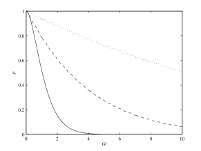
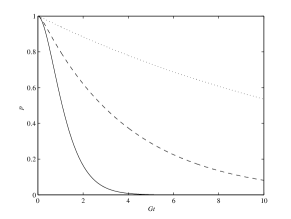
In Ref. art18 , two regimes were found for the dynamics of such a probability calculated by using the master equation corresponding to Hamiltonian (1) with resonant modes and :
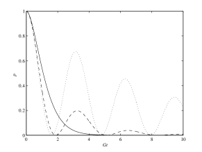
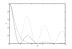
Here, the density operator stands for the state of the composed system . In one of the regimes, the increasing of the dissipation constant of mode leads to the decreasing of the permanence of the excitation in mode . This is expected, since mode is connected to the environment only through mode . The other regime was called Zeno regime: there, the increasing of the interaction of with the environment inhibits the transition of the excitation from to , leading to the enhancement of the probability of finding the excitation in . The turning point between these regimes occurs for , where is the unitary coupling constant between the modes of interest. In the Appendix, we show that such a turning point corresponds to , what is corroborated by Figs. (1a) and (2a). The occurrence of two regimes may be understood with the help of the following analytically calculable cases: for , ; for , . Depending on the relation between and , the dynamics can be approached to one of these limiting cases. By comparing Figs. (1a) and (2a) with Figs. (1b) and (2b), respectively, we see that the Hamiltonian and the master equation approaches exhibit good agreement. In order to achieve such an agreement, we have to pay attention to two aspects concerning the parameter : it must be large enough so that environmental modes with frequencies out of the interval have negligible action on the system (as pointed out in Ref. art19 , the relevant environmental modes are the ones with frequencies around the frequencies of the normal modes of the system ); the ratio must be small, allowing the use of the limit of dense spectrum.
II Sequence of Measurements
In this section we study the dynamics of two resonant coupled modes (, ) and atoms interacting, one at the time, with mode . The sequence of interacting atoms represents, in the limit of instantaneous interactions, a continuous measurement of the excitation number. The investigation shows that the two regimes reported in Ref. art18 and in the previous section are also present if a sequence of atomic interactions is performed on mode . These results illustrate the relation between continuous measurement of a quantum system and the dynamics governed by a master equation.
The results are obtained by numerical simulations, where we consider, as in Ref. art18 , the system of modes and in the initial state . A sequence of two level atoms interacts with mode . The atoms are prepared in the ground state and interact with mode one at the time. The Hamiltonian of the global system for the interaction of the -th atom is given by
| (14) |
where () and () are creation (annihilation) operators for modes and , their frequency, the modes coupling constant, , , and the coupling constant for the interaction between -th atom and mode . Here, and stand for the ground and the excited states of the -th atom, respectively.
After each interaction we perform the trace over the corresponding atomic system, i.e., we do not consider the final state of the atoms. We also assume that the coupling constant scales as , where is the interaction time of each atom art20 . The overall effect of these atomic interactions with a cavity mode is a dissipative evolution of the mode. The effective dissipative constant related to this process is .
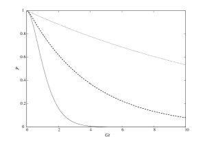
In Figs. (1c) and (2c) we shown two regimes for the probability of finding the excitation in mode (). In the dissipative regime (), the increasing of the dissipative constant leads to the decreasing of . In the second regime (), the increasing of the dissipative constant leads to the increasing of , preserving then the excitation in mode . It is worth to note that the agreement with the master equation results is reached in the limit of vanishing interaction time, . The increasing of interaction time leads the curves away from the ones obtained by the master equation.
III Conclusion
In the present work we investigate the two regimes of the system of two coupled modes, induced by two completely different dynamics. In the first one we consider the mode linearly coupled to a finite number of harmonic oscillators, and in the second one we consider such mode interacting with atoms, one at the time. Both dynamics, in appropriate limits, can describe the regimes obtained in art18 using a master equation. In the first model, when the number of harmonic oscillators goes to infinity the coupling between them and the system of interest can simulate the interaction with the environment. In the second model, the interaction with atoms, when the interaction time goes to zero, simulates continuous measurements. Therefore, the present results illustrate the idea that the interaction between system of interest and environment can be interpreted as continuous measurement on the system of interest. The results for both dynamics were obtained using numerical simulations. As no approximations were used in the calculations, the analysis of intermediate scenarios, out of the master equations limits, is possible.
IV Acknowledgements
This work was partially supported by the brazilian agencies CNPq and FAPEMIG.
Appendix A Establishing the relation between the effective dissipation constant and the parameters used in the Hamiltonian approach
The master equation employed in Ref. art18 is given by Eq. (I). It describes the dynamics of two linearly coupled resonant modes, one of them interacting with an environment at zero absolute temperature. Such a master equation may be derived as an approximation of the dynamics emerging from the Hamiltonian , leading, under the specifications in Eq. (8), to
| (15) |
where and is a value of beyond which the summations above are negligible art19 . For sufficiently large, we can take the limit of dense spectrum, resulting in
| (16) |
Since the integrand is assumed to be negligible for , we change for , which leads to
| (17) |
Observing that the term related to vanishes, we find, for ,
The transition to the Zeno regime were found in Ref. art18 for . This corresponds to
| (18) |

References
- (1) M. Schlosshauer, Rev. Mod. Phys. 76, 1267 (2005).
- (2) M. Simonius, Phys. Rev. Lett. 40, 980 (1978).
- (3) R. A. Harris, and L. Stodolsky, J. Chem. Phys. 74, 2145 (1981).
- (4) R. A. Harris, and L. Stodolsky, Phys. Lett. B 116, 464 (1982).
- (5) W. H. Zurek, Phys. Rev. D26, 1862 (1982).
- (6) R. Kubo, M. Toda, and N. Hashitsumi, Statistical Physics II: Nonequilibrium Statistical Physics, Springer Series in Solid-State Sciences, Vol. 31, Springer, Berlin, 1978.
- (7) B. Misra, and E. C. G. Sudarshan, J. Math. Phys. 18, 756 (1977).
- (8) W. M. Itano, D. J. Heinzen, J. J. Bollinger, and D. J. Wineland, Phys. Rev. A41, 2295 (1990).
- (9) L. E. Ballentine Phys. Rev. A43, 5165 (1991).
- (10) W. M. Itano, D. J. Heinzen, J. J. Bollinger, and D. J. Wineland, Phys. Rev. A43, 5168 (1991).
- (11) S. Pascazio, and M. Namiki, Phys. Rev. A50, 4582 (1994).
- (12) W. L. Power, and P. L. Knight, Phys. Rev. A53, 1052 (1996).
- (13) Jay Gambetta, et al., Phys. Rev. A77, 012112 (2008).
- (14) P. Facchi, and S. Pascazio, J. Phys. A: Math. and Theor. 49, 493001 (2008).
- (15) P. Facchi, and S. Pascazio, Phys. Rev. Lett. 89, 080401 (2002).
- (16) J. M. Raimond, et al., Phys. Rev. Lett. 105, 213601 (2010).
- (17) R. Rossi Jr., K.M. Fonseca Romero, and M.C. Nemes, Phys. Lett. A 374, 158 (2009).
- (18) Y. P. Huang, and M. G. Moore, Phys. Rev. A77, 062332 (2008).
- (19) J. D. Franson, B. C. Jacobs, and T. B. Pittman, Phys. Rev. A70, 062302 (2004).
- (20) S. Maniscalco, et al., Phys. Rev. Lett. 100, 090503 (2008).
- (21) R. A. Harris and L. Stodolsky, The Journal of Chemical Physics 74, 2145 (1981).
- (22) R. A. Harris and L. Stodolsky, Phys. Lett. B 116, 464 (1982).
- (23) Sabrina Maniscalco, Jyrki Piilo, and Kalle-Antti Suominen, Phys. Rev. Lett. 97, 130402 (2006).
- (24) A. R. Bosco de Magalhães, R. Rossi Jr., and M. C. Nemes, Phys. Lett. A 375, 1724 (2011).
- (25) R. Rossi Jr., A. R. Bosco de Magalhães, and M. C. Nemes, Phys. Lett. A 356, 277 (2006).
- (26) K. Jacobs, “Topics in quantum measurement and quantum noise”, Ph.D. Thesis, Imperial College, London, (1998).