An Operational Search and Rescue Model for the Norwegian Sea and the North Sea

Abstract

A new operational, ensemble-based search and rescue model for the Norwegian Sea and the North Sea is presented. The stochastic trajectory model computes the net motion of a range of search and rescue objects. A new, robust formulation for the relation between the wind and the motion of the drifting object (termed the leeway of the object) is employed. Empirically derived coefficients for 63 categories of search objects compiled by the US Coast Guard are ingested to estimate the leeway of the drifting objects. A Monte Carlo technique is employed to generate an ensemble that accounts for the uncertainties in forcing fields (wind and current), leeway drift properties, and the initial position of the search object. The ensemble yields an estimate of the time-evolving probability density function of the location of the search object, and its envelope defines the search area. Forcing fields from the operational oceanic and atmospheric forecast system of The Norwegian Meteorological Institute are used as input to the trajectory model. This allows for the first time high-resolution wind and current fields to be used to forecast search areas up to 60 hours into the future. A limited set of field exercises show good agreement between model trajectories, search areas, and observed trajectories for liferafts and other search objects. Comparison with older methods shows that search areas expand much more slowly using the new ensemble method with high resolution forcing fields and the new leeway formulation. It is found that going to higher-order stochastic trajectory models will not significantly improve the forecast skill and the rate of expansion of search areas.

Keywords

Search and rescue, operational forecasting, leeway, stochastic modelling, trajectory modelling.

Regional terms

North Atlantic, Norwegian Sea and North Sea.

1 Introduction

The Norwegian Joint Rescue Coordination Centres (JRCC) handle more than 1500 maritime incidents each year in the Norwegian Sea and surrounding waters. Of these incidents, a substantial part involves both search and rescue (SAR). This was the motivation for developing an operational search and rescue model that could be initiated with a minimum of information and that would rapidly return search areas based on prognoses of wind and surface currents.

Maritime search and rescue is essentially about estimating a search area by quantifying a number of unknowns (the last known position, the object type and the wind, sea state, and currents affecting the object), then compute the evolution of the search area with time and rapidly deploy search and rescue units (SRU) in the search area. This puts certain constraints on the model. First, the degrees of freedom must be limited to allow easy operation. This means that uncertainty about the last known position and assumptions on the shape of the object must be tractable for operational users in real time applications. Second, environmental data (wind and current fields, either prognostic, observed or climatological) must be available in real time and third, the model must be fast enough to make it an instrument for operative search area planning.

The motion of a drifting object on the sea surface is the net result of the balance of forces acting on it from the wind, the currents and the waves. In theory it is possible to compute the trajectory of an arbitrary drifting object given sufficient information on the shape and buoyancy of the object, the wind and wave conditions, and the surface current. In practice, the net motion is difficult to compute due to the irregular geometry of real-world objects. Simplifications must be introduced to make the problem tractable, and with these simplifications errors will also be introduced.

The drift brought about by the wind alone is termed the object’s leeway. We follow the definition by ?) that “The leeway is the drift associated with wind forces on the exposed above-water part of the object”. The aerodynamic force from the wind has a drag and a lift component due to the asymmetry of the overwater structure of the object [Richardson 1997]. The drag is in the relative downwind direction, whereas the lift is perpendicular to the relative wind direction and will cause the object to diverge from the downwind direction. Likewise, the hydrodynamic force on the submerged part can be decomposed into a lift and a drag component. The hydrodynamic lift will balance the lateral (perpendicular to the drift direction) component of the aerodynamic force and prevent the object from toppling sideways. The lift gives rise to a significant crosswind leeway component for elongated objects. This phenomenon is most commonly observed with sailboats that indeed are designed to sail up against the wind [Kundu 1990, pp 575–576]. The object’s initial orientation relative to the wind (left or right of downwind) will set the object off along different paths. As the initial orientation is essentially unpredictable equal probability must be assigned to the two outcomes.

Another source of uncertainty lies in the wind and current data, modelled or observed. The fields will always contain errors. Additionally, fluctuations on a scale smaller than those resolved by the forecast models or observing systems will always be present. The phenomenon is often referred to as sub-grid scale in numerical modelling. Similarly, observing systems will also have temporal and spatial resolution issues, often referred to as the error of representativeness [Daley 1991, p 12]. These unresolved and unobserved small scale fluctuations will affect the drifting object and must be quantified and taken into account when estimating its motion. The forces acting on an object on the sea surface are discussed in Sec 2 along with the simplifications and approximations employed.

It is obvious that there is a large ingredient of chance involved in the calculation of an object’s motion on the sea surface, thus a probalistic formulation is necessary to tackle the uncertainties involved. Rather than forecasting the exact trajectory of the object, a most probable area is sought, i.e., an evolving probability density function in space. We employ a Monte Carlo technique to compute the probability density function (interpreted as the search area) for the location of the object by perturbing the different parameters that have a bearing on the object’s trajectory. The ensemble (Monte Carlo) trajectory approach is discussed in Sec 3.

The problem is made even more complicated when we go from modelling the drift of a known object from a last known position to searching for a possibly unknown object with scarce information on its last known position. Here, a geographic area and a time period enter the suite of uncertainties along with the unknown drift properties of the object at large. Sec 3 describes the implementation of the operational search model Leeway.

The Leeway model is part of a suite of oceanic trajectory models including a ship drift model and a three dimensional oil drift model. The models are developed and operated by the Norwegian Meteorological Institute for the operational community (search and rescue and vessel traffic service and the enviromental protection agency). A description of the complete trajectory model suite is given by ?).

An earlier Monte Carlo based search model has been successfully used in maritime search operations since the early seventies when the US Coast Guard developed its “Computer assisted search program” (CASP). For a review of the developments in this field, see ?). The major difference between earlier Monte Carlo based SAR models and our approach is the quality of the atmospheric and oceanographic fields (e.g., real-time currents yield lower error variance than climatological currents typically used in earlier systems) and the formulations of the leeway coefficients, which are here decomposed into the more robust downwind and crosswind components rather than a leeway divergence angle (discussed in Sec 2.1)

Sec 4 discusses some results obtained with the model, the limitations of the theory, the quality of the operational tool, and possible future extensions.

2 The forces on a drifting object

An object on the sea surface will accelerate as

$$(m+m^{\prime})\frac{d\mathbf{V}}{dt}=\sum\mathbf{F},$$ (1)

where $\mathbf{V}$ is the object velocity and $\sum\mathbf{F}$ is the sum of the forces. The added mass $m^{\prime}$ comes from the acceleration of water particles along the hull of the object ([Hodgins and Hodgins 1998], [Mei 1989], [Richardson 1997]).

Life rafts are observed by ?) to reach terminal velocity in approximately 20s under strong wind conditions (20m/s). This implies that small objects (typically less than 30 m) accelerate very rapidly. This is confirmed by ?) who found the highest cross-correlation between leeway speed and wind speed at zero lag for 10-minute vector averaged samples. Infinite acceleration and constant velocity for the duration of a model time step are thus acceptable simplifications. The length of the model timestep is then dictated by the temporal and spatial scale of the forces acting on the object (wind, waves and currents). These vary over much longer timescales (surface currents, including tidal motion, and the synoptic weather situation change appreciably in hours, not minutes).

2.1 Wind and leeway

We define the leeway (windage) of an object to be the drift associated with the wind force on the overwater structure of the object as measured relative to the 10 minute averaged wind measured at 10 m height (or reduced to this height). This coincides with the meteorological convention for measuring surface wind and is consistent with earlier work in this field ([Hodgins and Mak 1995]). It is observed that an object moving under the influence of the wind will diverge to some extent from the downwind direction due to balance between the hydrodynamic lift and drag of the subsurface area and the aerodynamic lift and drag of the wind.

The empirical relation between leeway and wind speed presented here is based on field work carried out by or compiled from other sources by the U.S. Coast Guard. The empirical coefficients are summarised in ?). A total of 63 different search leeway categories has been compiled (discussed further in Sec 3.4, see also Table 1). Leeway field experiments endeavour to determine the relation between the wind speed and the leeway speed and divergence angle, $L$ and $L_{\alpha}$, or more robustly, the downwind (DWL) and crosswind (CWL) leeway components, $L_{\mathrm{d}}$ and $L_{\mathrm{c}}$ (see Fig 1). The latter parameters are more stable to directional fluctuations at low wind speed and are therefore preferred. To achieve this, it is necessary to combine wind measurements from a nearby buoy with GPS measurements of the motion of the object (over 10 minute intervals) and current measurements of the slippage (the object’s motion relative to the current at a certain level, discussed below). The empirical coefficients for leeway speed and the divergence angle listed in ?) were converted by ?) into downwind and crosswind components of leeway as functions of the 10 m wind speed. The decomposition into downwind and crosswind coefficients are implemented for the first time in the operational model described in this work.

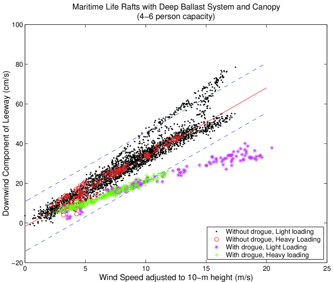
Figure 2: Measured downwind component of leeway, $L_{\mathrm{d}}$ of maritime life rafts with deep ballast systems, canopy, and capacity 4–6 persons relative to the 10 m wind speed, $W_{10}$. The leeway measurements are wind only, the wind-induced drift is subtracted from the measurements using surface current measurements. The linear regression $\widehat{L}_{\mathrm{d}}$ and its 95% confidence limits are also indicated. Note the influence of the drogue (sea anchor, marked with asterisks in pink and green) on the leeway. The experimental variance is also a function of the wind speed (hetereoscedasticity, i.e., the spread is greater for higher wind speeds). [from Allen and Plourde, 1999].

The experimental data shown in Fig 2 suggest an almost linear relationship between wind speed $W_{10}$ and the downwind component of the leeway. This linear relationship is also observed by other workers (see [Richardson 1997]; [Hodgins and Hodgins 1998]). The downwind and crosswind leeway measurements described in Figs 2 and 3 are corrected for wind-induced drift by measuring the slippage.

A linear regression with least squares best fit coefficients is now computed to relate $L_{\mathrm{d}}$ to the local wind speed,

$$\widehat{L_{\mathrm{d}}}=a_{\mathrm{d}}W_{10}+b_{\mathrm{d}}.$$ (2)

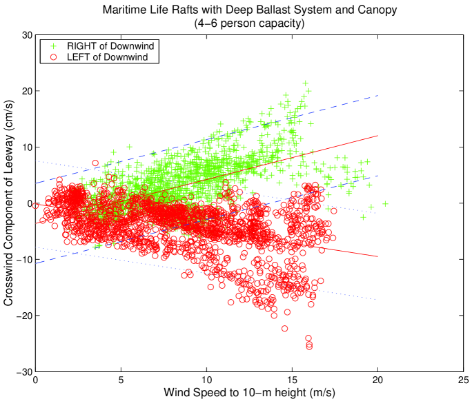
Figure 3: Same as Fig 2 for the crosswind component of leeway. The leeway measurements are wind only, the wind-induced drift is subtracted from the measurements using surface current measurements. Drifting objects can move at a relative angle left (red) or right of downwind (green) (from Allen and Plourde, 1999).

Here, $a_{\mathrm{d}}$ and $b_{\mathrm{d}}$ are regression coefficients determined from the experimental data and $\widehat{L_{\mathrm{d}}}$ is the estimated best fit DWL. An analogous derivation applies to the crosswind component of the leeway, $\widehat{L_{\mathrm{c}}}$. The dataset is divided into left-drifting and right-drifting observations, depending on whether the object was observed to bear to the left or to the right of the local downwind direction (see Fig 3). Note that the regression coefficients are similar but not identical for the left and right drifting objects. The data suggest that left and right drifting observations are almost equally probable, hence in the following we assume a 50/50 distribution.

The 10 m wind fields used in the operational ensemble trajectory model described later are taken from the High Resolution Limited Area Model (HIRLAM), the numerical weather prediction model of The Norwegian Meteorological Institute. The model has a horizontal resolution of approximately 20 km on a rotated spherical grid. The model and assimilation is run four times daily (00, 06, 12, 18 UTC). Each model integration extends to +60 hours. The current version of the HIRLAM model is described by ?). Open boundary conditions are taken from the Integrated Forecast System (IFS) of The European Centre for Medium-Range Weather Forecasts (ECMWF).

2.2 Current and slippage

The current vectors used in this study are taken at 0.5 m depth. This coincides with the draft of typical SAR objects and roughly with the depth at which current meters are mounted in leeway field experiments. The slippage of an object is defined as its motion relative to the ambient current at a certain depth comparable to the draft of the object (set to 0.5 m in our case). In the absence of wind, the object is assumed to move with the local surface current, $\mathbf{u}_{\mathrm{w}}$, i.e., no slippage. The object is further assumed to adjust its motion instantaneously when the current changes (infinite acceleration, discussed above).

Surface current fields in the operational setup of the Leeway model described in Sec 3 are taken from the operational 3D baroclinic ocean model of The Norwegian Meteorological Institute. The model is a modified version of the Princeton Ocean Model (POM) with 4 km horizontal resolution on a polar stereographic Arakawa C grid. The model solves numerically the primitive equations of motion (with Boussinesq and hydrostatic approximations) along with equations for the conservation of heat and salt. A Mellor-Yamada turbulence closure scheme is employed for the vertical eddy viscosity [Mellor and Yamada 1982]. The model is driven by atmospheric forcing (10 m wind, heat flux, and atmospheric pressure) from an operational atmospheric model (see above) and all major tidal constituents on the open boundary. The original model formulation is described by ?).

The vertical dimension is resolved by 21 unevenly spaced (higher resolution near the surface and the bottom) layers of terrain-following $\sigma$-coordinates. The uppermost layer of the model is $0.001H$, where $H$ is the depth. Coastal waters are thus well resolved vertically (e.g., the uppermost layer is 0.3 m below the sea surface in 300 m deep waters). For our purposes current vectors have been interpolated to 0.5 m below the sea surface for consistency with the field experiments carried out to establish leeway coefficients.

Climatological river runoff is included in the model. The river runoff has a strong seasonal signal and makes an important contribution to the coastal circulation.

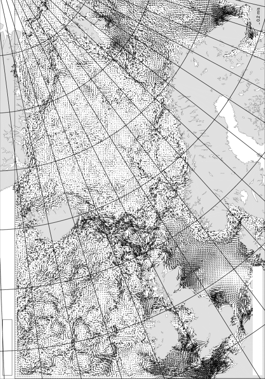
Figure 5: Modified Princeton Ocean Model domain operated by The Norwegian Meteorological Institute. Current vectors at 0.5 m below sea surface are shown. The model has a horizontal resolution of 4 km (every fourth vector shown, $5^{\circ}\ \,$graticule). The ocean model is forced with 20 km resolution 10 m winds from the HIRLAM numerical weather prediction model. All major tidal constituents are prescribed on the boundary. Daily prognoses out to +60 h are initiated at 00 UTC. The operational setup of the leeway model is confined to the ocean model grid. A seven day archive allows trajectory calculations to be inititated several days after the event occurred.

The model and the operational setup at the Norwegian Meteorological Institute is described in detail in ?) and ?). The model grid is outlined in Fig 5.

2.3 Wave effects ignored

The Stokes drift is a downwave drift induced by the orbital motion that water particles undergo under the influence of a wave field. These particle orbits are not closed and a Lagrangian drift is set up. This drift is confined to a narrow layer next to the sea surface [Kundu 1990, pp 223–225]. It is well known that the Stokes drift can be a dominant factor in the advection of suspended material and objects on the sea surface.

In the field campaigns conducted to estimate leeway coefficients (reviewed in [Allen and Plourde 1999]), the wind and the near-surface current were the only measured quantities apart from the object’s motion. The Stokes drift is predominantly down-wind and is difficult to separate from the direct wind effect on the object after the ambient current has been subtracted because it is a Lagrangian effect invisible to the Eulerian current measurements that were collected in the field experiments. Thus, even though the Stokes drift is readily available from operational wave models such as WAM (see [Hasselmann, Hasselmann, Bauer, Janssen, Komen, Bertotti, Lionello, Guillaume, Cardone, Greenwood, Reistad, Zambresky, and Ewing 1988]), it is necessary to leave it out as it is assumed to be already present in the empirical leeway coefficients.

The Stokes drift can also significantly modify the upper layer velocity through interaction with a sheared near-surface current. This interaction generates Langmuir circulations, i.e. vortices parallel to the wind direction (see [Skyllingstad and Denbo 1995] and [Carniel, Sclavo, Kantha, and Clayson 2005]). No attempt has been made at estimating the wave-current effect on the near-surface currents as this is numerically very demanding. It requires an estimate of the Stokes drift derived from a wave forecasting model which in turn must be added to the momentum equations of the ocean model. However, it is clear that this effect may become important, particularly in high seas and a strong vertically sheared current.

Wavelengths comparable to the object dimension are most efficient in transferring energy to the drifting object [Hodgins and Hodgins 1998]. The wave force in this regime ($\lambda\sim D$) for a fixed object simplifies to

$$\mathbf{F}_{\mathrm{wave}}=\frac{1}{4}\rho ga^{2}D.$$ (3)

Here, $a$ represents the amplitude of the energy found in a narrow spectral band covering the dimension $\lambda=D$ [Mei 1989]. Note that the energy transmitted to a drifting object is even smaller than in the case of a fixed object. We assume that damping and excitation is negligible for small objects (less than 30 m length) with no way on, even in a well developed sea (see [Komen, Hasselmann, and Hasselmann 1984], [Sørgård and Vada 1998], and [World Meteorological Organization 1988]. Wave effects are therefore ignored for all objects treated in this work. It can further be argued that as waves are wind-driven (ignoring the negligible effect of swell on smaller objects), the wave force will be aligned with the wind. This will lead to a small downwind force which will be difficult to disentangle from the field data for the empirical leeway coefficients as no direct wave measurements have been performed [Allen and Plourde 1999].

2.4 Total motion

Following the assumptions and simplifications above, the trajectory model simplifies to calculating the arc traced by the leeway vector superposed on the surface current,

$$\mathbf{x}(t)-\mathbf{x}_{0}=\int_{0}^{t}\mathbf{V}(t^{\prime})\,dt^{\prime}=\int_{0}^{t}\left[\mathbf{L}(t^{\prime})+\mathbf{u}_{\mathrm{w}}(t^{\prime})\right]\,dt^{\prime}.$$

A second order Runge-Kutta scheme is used for the computation of trajectories on a sphere.

3 The operational ensemble trajectory model

In searching for drifting objects on the sea surface, we are faced with the challenge of quantifying a large number of unknowns and to estimate a most probable search area in light of these uncertainties. A search operation attempts to maximize the probability of success ($POS$), which in turn depends on the probability of detection ($POD$) and the probability of containment ($POC$),

$$POS=POD\times POC.$$

$POC$ is the a priori search area, i.e. the area that most likely contains the drifting object. Leeway, the operational SAR model described here yields search areas ($POC$) and does not involve the probability of detection, which depends on the resources available, the visibility in the area and other external factors. It is the task of the rescuers to take the information from $POC$ and apply their resources ($POD$) to maximize $POS$. In addition to perturbing the leeway coefficients and the forcing fields, an operational model must perturb the initial position and the initial release of the object to account for the uncertainty in last known position.

The linear leeway relation described in Sec 2.1 can be superposed on surface current data (prognoses, measurements, or climatology, depending on what is available) to estimate the trajectory of a drifting object. However, as was mentioned in Section 1, there are several sources of uncertainty and errors that will cause the true and modelled trajectories to diverge with time. Consequently, an evolving probability density function in the two lateral dimensions (longitude and latitude) is sought. The approach chosen here is to estimate the errors and uncertainties and to perform a Monte Carlo integration by rerunning the trajectory model multiple times with all relevant parameters perturbed to generate an ensemble.

To motivate the use of the Monte Carlo technique, we start by assuming that the position of a drifting object behaves as a Markov process or first order autoregressive process,

$$p(\mathbf{x}_{t+1}|\,\mathbf{x}_{t},\mathbf{x}_{t-1},\mathbf{x}_{t-2},\ldots,\mathbf{x}_{1})=p(\mathbf{x}_{t+1}|\,\mathbf{x}_{t}),$$ (4)

i.e., the probability density function of the future state is only dependent on the current state and not on the particular way that the model system arrived at this state (see [Wilks 1995], p 287 or [Priestley 1981], p 117). Here, $\mathbf{x}$ represents the state of the system (in our case the “state” is simply the location of the drifting object and whether it is drifting or stranded). Let $\mathbf{V}$ represent the (possibly nonlinear) function for the displacement of the object under the influence of external forces. Embedded in $\mathbf{V}$ is the external forcing (wind and current) as well as the drift properties of our particular object. The random perturbations $d\boldsymbol{\epsilon}$ have a known covariance and zero mean. These represent the uncertainties in drift properties and forcing (wind and current). Under the assumption that the perturbations behave as a Markov process, the trajectory evolves as

$$d\mathbf{x}=\mathbf{V}(\mathbf{x},t)dt+d\boldsymbol{\epsilon}.$$ (5)

The ensemble consists of $\mathcal{O}(N)$ samples drawn from the stochastic differential equation (5).

3.1 Leeway coefficient perturbations

The orientation (left and right of wind) of the ensemble members is distributed equally and remains fixed throughout the integration. This means that a member will not “jibe”, i.e., once started to the left of downwind it will continue on that tack throughout the simulation.

The perturbations in leeway coefficients are supposed to cater for the properties unique to the object (e.g., is this a less than normally loaded life-raft, or does the raft sag?). It is important to note that the perturbations in leeway properties remain fixed throughout the simulation.

It is clear from the experimental data compiled by ?) that the variance increases with wind speed, i.e., the dataset is slightly heteroscedastic (see Figs 2 and 3). This should be accounted for, and to recreate the spread about the regression (2) both the slope and the offset of the regression line of ensemble members $n=1,\ldots,N$ is adjusted by adding a common perturbation $\epsilon_{n}$ drawn from a normal distribution $N(0,\sigma)$,

$$a_{n}=a+\epsilon_{n}/20,$$ (6)

$$b_{n}=b+\epsilon_{n}/2.$$ (7)

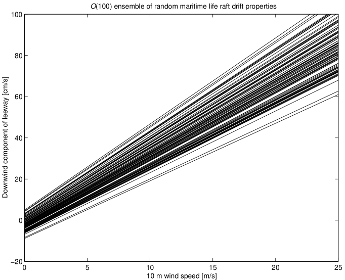
Figure 4: $\mathcal{O}(100)$ random perturbations of the downwind leeway component of the maritime life raft found in Fig 2. Both the slope and the offset are perturbed to allow the ensemble to reproduce the heteroscedastic spread about the best fit linear regression, $L_{n}=(a+\epsilon_{n}/20)W_{10}+(b+\epsilon_{n}/2)$.

At $W_{10}=10$m/s, equal perturbations are added to slope and offset, $L=(a+\epsilon_{n}/20)W_{10}+(b+\epsilon_{n}/2)$. At lower wind speeds the bulk of the perturbation is contributed by the offset ($b+\epsilon_{n}/2$), whereas at higher wind speeds the slope adds most. Fig 4 illustrates an ensemble of simulated regression lines drawn from Eqs (6) and (7).

3.2 Wind and current perturbations

Ignoring higher-order dispersion

Higher-order stochastic particle dispersion models and their applicability to surface drifting objects with little or no leeway have been studied extensively by, among others, ?) and ?). The models are all Markov processes of different orders. The successor to the “random walk” or Markov-0 model presently employed by our trajectory model is the “random flight” formulation. This transport model allows fluctuations to slowly evolve. The integral time scale $\mathcal{T}$ is a measure of the memory of the perturbations. It is related to the autocorrelation of the velocity field through

$$\mathcal{T}=\int_{0}^{\infty}R(\tau)\,d\tau.$$

An exponential autocorrelation function is normally assumed,

$$R(\tau)=e^{-\tau/T}$$

[Griffa 1996]. Upper ocean current fluctuations are correlated and $\mathcal{\mathcal{T}\sim}2$ days [Griffa 1996, Poulain 2001].

SAR objects are influenced by both the wind and the surface currents. Ideally, correlated fluctuations in the wind speed and direction should also be accounted for. ?) found that wind gusts obey a first order auto-regressive formulation similar to the random flight formulation for surface drifters. A coefficient of approximately 0.9 is found to be appropriate to add gusts to six-hourly winds to force a wave model.

A random flight formulation based on estimates of the integral time scale for both the surface current fluctuations and the wind fluctuations would represent the next level of sophistication in our ensemble trajectory model. This approach has been tested with good results for passive drifters with negligible leeway by ?). The drifter trajectories were estimated using currents from a chain of high-frequency radars. Estimates of the integral time scale and the upper ocean diffusion were available from the HF radar data. However, estimating the integral time scale of surface current fluctuations and wind fluctuations in different geographic areas and for different seasons can be difficult. As we have developed an operational model whose primary task is to estimate the location and magnitude of search areas for an array of search objects, we argue that it is better to keep the model simple pending reliable estimates of the turbulent time scales of the upper ocean and the atmospheric boundary layer.

However, the most compelling argument for retaining a simple stochastic model is the enormous dispersion caused by the experimental error variance of the leeway properties of SAR objects with appreciable windage (which includes all typical SAR objects, even persons in water). As perturbations to leeway coefficients must be constant in time for each ensemble member (otherwise the members representing drifting objects would have drift properties that changed with time, which is clearly unrealistic), these contribute two orders of magnitude more to the dispersion than the time-varying wind and current perturbations. Model tests with wind standard deviation 2.6m/s and current standard deviation 0.25m/s yield almost the same ensemble spread (less than 2% difference after $\mathcal{O}(250)$ timesteps, not shown) as simulations where the wind and current perturbations were turned off. Thus wind and current induced dispersion is swamped by the dispersion caused by the perturbations to the leeway coefficients. Obviously, regions with strong current shear or sharp atmospheric fronts will cause the ensemble to diverge more rapidly than under stable and homogeneous conditions. In general, though, it is reasonable to assume that wind and current perturbations are of secondary importance and that a random flight dispersion model will not have discernible impact on the rate of expansion of the search area.

A random walk wind perturbation model

Consequently, perturbations $\mathbf{u}^{\prime}$ of the wind field are assumed to follow a circular normal distribution,

$$\mathbf{u}^{\prime}_{n}\equiv(u_{n}^{\prime},v_{n}^{\prime})\in N(0,\sigma_{W}),$$ (8)

$$W_{n}\equiv\left\|\mathbf{W}_{10}+\mathbf{u}_{n}^{\prime}\right\|_{.}$$ (9)

The ensemble of leeway components becomes

$$L_{n}=a_{n}W_{n}+b_{n},\>n=1,\ldots,N,$$ (10)

Again, identical derivations hold for the downwind and crosswind equations, and subscripts to distinguish the two are left out for brevity. The perturbations $\mathbf{u}_{n}^{\prime}$ are uncorrelated in time. Sub-grid scale fluctuations appear as errors in comparisons between model prognoses and observations. These fluctuations must be accounted for as the sub-grid scale affects the drifting object. The zeroth order approach to adding sub-grid scale effects is to use uncorrelated perturbations (random walk). A possible extension to allow time-coherent (random flight) fluctuations is discussed in Sec 4.

Based on wind observations and the 12 h prognosis at Ocean Weather Station Mike ($66^{\circ}$N, $002^{\circ}$E), we have estimated the 12 h forecast RMS error to be $\sigma_{W}=2.6$m/s in both the east and the north components (not shown) of the wind vector.

3.3 Release time and initial position

The first task in a search is to determine the object’s initial position in time and space, i.e., the position and point in time where the object started drifting with no way on. If the last known position (LKP) is assumed to be rather precise (e.g., a distress call is received from a ship with a GPS unit), a small radius of uncertainty may be assigned to this position and consequently all ensemble members will be released simultaneously and within short distance of each other. In the other extreme, take a situation where little is known about the time and location of the accident. Then a wide radius and a long release period must be used. This will result in a large cloud of candidate positions at later times. The various members of the ensemble will endure very different fates due to the spatial and temporal variation in current and wind fields. It is obvious that the choice of initial distribution of ensemble members will greatly affect the future search area. Eight degrees of freedom are available for defining the initial distribution in the current implementation of Leeway:

• Date-time, $t_{0},$ position, $\mathbf{x}_{0}$ (latitude and longitude), and radius of uncertainty, $r_{0},$ of the earliest possible time of accident

• Date-time, $t_{1},$ position $\mathbf{x}_{1},$ and radius of uncertainty, $r_{1},$ of the latest possible time of accident

The ensemble size $N$ is $\mathcal{O}(500)$. All initial positions are drawn from a circular normal distribution with standard deviation $\sigma=r/2$, where the radius $r$ is varied linearly between $r_{0}$ and $r_{1}$. This approach is flexible, it allows on one hand for point release in space and time and in the other extreme one can seed particles continuously in a “cone” shaped area with one radius of uncertainty in one end and another radius in the other end of the seeding area. Fig 6 gives an example of a general, cone shaped initial distribution. By setting $r=2\sigma$, approximately 86% of the particles are released within the radius.

3.4 Object taxonomy

The drift properties of typical maritime search objects have been studied extensively since World War II. In Table 1 we present only a truncated list of the relevant SAR objects discussed by ?). Some categories are further divided into subclasses. Generic classes are created by uniting different datasets and increasing the experimental variance accordingly. Note that the quality of the experiments, and thus the error variances, varies widely, depending on the equipment and methods used to conduct the experiments.

Fig 7 illustrates qualitatively the difference in drift properties between typical search objects, in this case a life raft and a sail boat, and how this leads to very different search areas as time progresses. Notice the significant leeway divergence angle of the sailboat and how this produces two disjoint search areas, depending on whether the boat drifts to the left or the right of the wind. The life raft, on the other hand, moves somewhat faster and with much less divergence, making the overall search area smaller through overlap. Fig 7 also demonstrates the importance of redoing leeway field work using modern techniques; the smaller search area of the life raft search area is in part a consequence of the lower experimental variance achieved in using modern field experiments.

4 Discussion and outlook

4.1 Drift exercises

Controlled experiments to evaluate the performance of the operational model are lacking. However, a few incidents have been reported and a few exercises conducted that yield some information about the forecast skill of the model. We describe here three cases reported to us by the Norwegian Rescue Co-ordination Centres and one specifically modelled. We stress that these cases do not constitute a model evaluation and serve merely as illustrations of the ability of the model to reproduce the observed trajectories.

Benthic lander

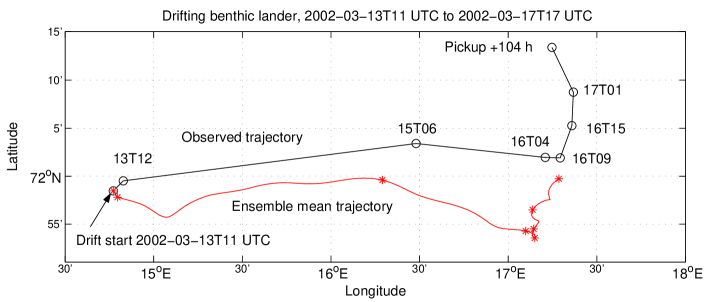
Figure 8: The trajectory of a benthic lander off the coast of Northern Norway. ARGOS positions marked with (o) and date-time. Lower curve represents the ensemble mean model trajectory. Intermediate positions coincident with times of observations are marked with (*). The lander drifted for more than four days over which the general features of the trajectory were well captured by the model.

A benthic lander released itself from the sea bed on 2002-03-14T11 UTC after a malfunction. Its position was tracked irregularly (observations are marked with date and time in Fig 8) by the ARGOS network over the following days until it was picked up on 2002-03-17T17 UTC. As Fig 8 shows, the average trajectory using the class “person in water, mean values” (PIW-1) corresponds quite well with the observed intermediate positions (compare the asterisks on the ensemble mean trajectory with the observed positions, marked with date and time.

Faroe-Iceland exercise 2003

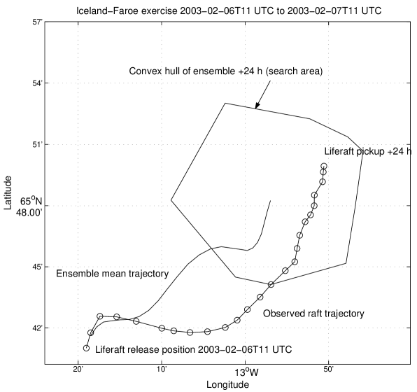
Figure 9: Average trajectory v observations. A liferaft was tracked for 24 hours, its GPS positions are marked with (o). The ensemble mean model trajectory compared reasonably well with the intermediate positions. The search ended after 24 hours. By then the search area, illustrated by the convex hull of the ensemble, had expanded to approximately 90 $\textrm{nm}^{2}$.

A liferaft was released on 2003-03-21T10 UTC as part of an exercise conducted by the Faroese, Icelandic, and Norwegian rescue services. Its position was tracked for 24 hours using GPS. As Fig 9 shows, the liferaft was picked up near the center of the search area. The ensemble mean trajectory agreed well with the intermediate positions.

Comparison of search methods: Faroe-Iceland exercise 2004

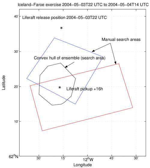
Figure 10: Comparison of search methods. Three search methods were used to forecast the search area for a liferaft 16 hours after its release. The two search areas marked “manual search areas” were computed using the standard methods employed by the Icelandic and Faroese SAR organizations. These methods rely on climatological surface currents and low-resolution wind forecasts. The search ended after 16 hours. By then the search area, illustrated by the convex hull (the polygon) of the ensemble, had expanded to 100 $\textrm{nm}^{2}$, significantly smaller than the manual search areas.

A liferaft was released on 2004-05-04T08 UTC through a joint exercise between the Faroese, Icelandic, and Norwegian rescue services. The pickup position and search areas computed using three different methods are shown in Fig 10. The search area based on the Leeway model is marked with black. As can be seen the raft is picked up near the centre of the search area. A comparison with search areas computed by the Faroe and Icelandic rescue services (red and blue) suggests that the rate of expansion of search areas based on the Leeway model is 25-50% of that using older methods. No intermediate positions of the raft were available.

4.2 Possible model extensions and improvements

The Leeway model is built primarily for operational purposes. As such it must be fast, easy to operate (limited degrees of freedom), and it must not underestimate the rate of expansion of search areas. Here we investigate possible extensions to the model which may have an impact on the precision and the rate of expansion of the search areas.

Improved object taxonomy and leeway coefficients

The leeway categories available today are a compilation of all the field experiments performed by the US Coast Guard, the Canadian Coast Guard, and other search and rescue services around the world (see Table 1). The datasets are of various quality and some object classes have a very high error variance (see the example in Fig 7). Such classes have not been studied with modern field equipment and should be redone. It is important to note also that because the perturbations to the drift properties are time-invariant, they contribute much more than the random walk added to the wind field. Lowering the experimental variance of the leeway coefficients for a search object translates directly into a reduced the rate of inflation of the search area.

Several object classes are clearly missing as each country with a coastline has its own particular SAR objects, e.g., fishing boats endemic to the region. There are also many world-wide SAR categories that would benefit from further refinement, e.g., the various brands of life rafts.

Jibing, swamping and capsizing

The empirical trajectory model described in Sec 2 computes the linear displacement of a SAR object by the wind and the currents. In reality, a drifting object in rough weather will experience both breaking waves and strong wind gusts. The object may jibe, swamp, or capsize under such conditions. No attempt has been made at trying to include these effects as experimental data are scarce. However, with dedicated experiments it may be possible to quantify the probabilities of jibing, swamping, and capsizing for different SAR objects.

Jibing has been observed to occur at very low wind speeds and at very high wind speeds. It may be assumed that there is a small, but finite, probability that an object will jibe under intermediate wind conditions [Allen 2005]. The effect of including jibes will be a more continuous search area as some ensemble members will “change sides” and fill in the gap between the two distributions.

Swamping and capsizing affect the leeway of the object drastically. Assigning probabilities of capsizing and swamping under different weather conditions would contribute toward making the search area more realistic. For now, lack of experimental data prevents a thorough assessment of the frequency of swamping and capsizing for different categories of SAR objects.

Increased ocean model resolution

Although it is by no means certain that higher resolution leads to higher precision in ocean modelling, increasing the horizontal resolution is important for two reasons.

First, even at 4 km resolution the model is only beginning to resolve the eddy activity of the upper ocean. Moving towards 1-2 km resolution will finally yield a realistic current spectrum. Resolving eddies means that a cloud of particles (or ensemble) will disperse more realistically, even if the eddies are not located correctly in time and space.

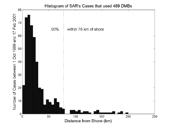
Figure 11: Number of US Coast Guard SAR cases involving datum marker buoys between 1999-10-01 and 2001-02-17 and their distance to shore.

Second, the vast majority of rescue operations take place less than 40 km (25 nm) from shore. Shown in Fig 11 is the distribution of self-locating datum marker buoy (SLDMB) with distance from shore in incidents in US waters. The buoys are deployed to assess the speed and direction of the surface current near the last known position of a search object and thus indicate the typical seaward distance of incidents. Obviously, surface current fields that resolve the near-shore currents well will greatly enhance the value of an operational SAR model. For complex coastlines (the Norwegian is a prime example) detailed current fields are required to realistically model the flow between islands and in the mouths of fjords and estuaries.

4.3 Conclusion

We have presented a new operational model for the evolution of search areas for drifting objects. A taxonomy of common SAR objects has been set up based on the field experiments conducted to date.

A new method for decomposing and perturbing the leeway of the object in downwind and crosswind components has been employed, yielding more robust computations at low winds and more realistic ensemble perturbations. It is found that this new method makes search areas inflate at approximately 25-50% of the rate found using older methods. The stochastic particle trajectory approach employed for this model thus leads to a significantly lower rate of expansion of search areas compared with other models.

The ensemble trajectory model is operational and can forecast search areas up to 60 hours ahead in time. A seven day archive of wind and current fields allows simulations to be started as early as one week ago. This is important, as incidents are not always reported immediately.

It is found that particles are dispersed primarily through the perturbation of leeway properties, as these remain constant for each individual ensemble member. The added dispersion from perturbations (random walk) of the wind field and the current field is negligible in comparison. Going to a higher-order stochastic particle model is found to make very little difference to the rate of expansion of search areas. Thus a random walk model for the perturbations of wind and current fields is sufficiently sophisticated to capture the evolution of search areas given the high dispersion caused by the time-invariant leeway coefficients.

The vast majority of rescue operations at sea occur close to the coast. We have argued that further increasing the horizontal resolution of the ocean model will allow the model to assist searches even nearer the shore and in major bays and fjords while at the same time making the ensemble spread more realistically as eddy motion becomes more adequately resolved.

More field work is required to adequately model the various SAR objects frequently found in Norwegian waters and elsewhere. Furthermore, the experimental error of some of the older leeway categories is so high that it is desirable to revisit these SAR objects by conducting new and improved field experiments.

We have a limited, yet convincing set of field trials where the model has been compared with trajectories and end positions of real SAR objects (life rafts). The model succeeds in capturing the features of the trajectories of several drifting objects. Further studies will be required before definite conclusions can be drawn about its forecast skill, but the results so far are promising.

Acknowledgments

This work was supported by the Norwegian Ministry of Justice, The Norwegian Joint Rescue Coordination Centres (JRCC), and The Royal Norwegian Navy through the project “Drift av gjenstander” (Drifting objects) and subsequent follow-up projects. The JRCC also contributed directly to this work by making the data from their field exercises available. The Research Council of Norway and the French-Norwegian Foundation (Eureka grant E!3652) supported the development of the operational service through the SAR-DRIFT project. The U.S. Coast Guard has generously made all their compiled leeway field data available.

Figures

Figure 1: The leeway $\mathbf{L}$ of a drifting object consists of a downwind component (DWL), $L_{\mathrm{d}}$, and a crosswind component (CWL), $L_{\mathrm{c}}$. The angle between the downwind direction and the leeway drift direction is termed the leeway divergence angle, $L_{\alpha}$ [adapted from Allen and Plourde, 1999].

Figure 6: Seeding the ensemble. The initial distribution of ensemble members in space is defined by two circles with radii $r_{0}$, and $r_{1}$, centred on positions $(\phi_{0},\lambda_{0})$ and $(\phi_{1},\lambda_{1})$, respectively. Members (marked as black particles) are seeded randomly in the area outlined by the two great circle arcs (representing $2\sigma$, which is why some particles lie outside the arcs). Members are released continuously between $t_{0}$ and $t_{1}$, the first near position 0, the last near position 1. This allows us to define accidents where the time of the accident is uncertain while simultaneously assuming that the vessel is under way. Simpler scenarios can be defined by setting start and end positions equal og reducing the time period to a point release.

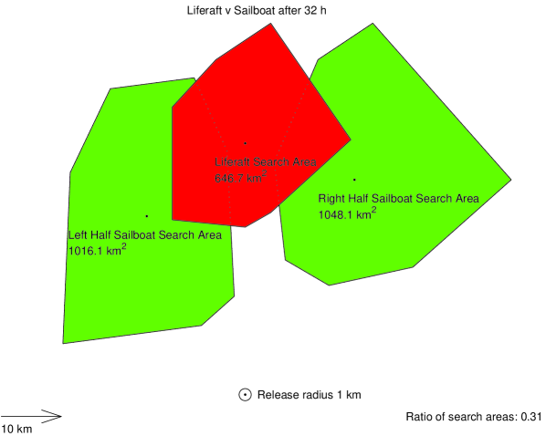
Figure 7:

The simultaneous search areas of a modern life raft with deep ballast system and a sailboat at time $t=+32\textrm{ hours}$ are shown as polygons. The average wind speed was 10m/s in this simulation. The polygons are convex hulls that encompass the individual ensemble members (not shown). All ensemble members representing both search objects were released simultaneously in the same radius ($r_{0}=r_{1}=$1 km). The sailboat search area is significantly larger than the liferaft search area (left and right lightly shaded polygons). This is in part due to higher divergence which causes the search area to split in two after a while. The liferaft search area (dark grey, centre), on the other hand, is still contiguous as modern liferafts have only a small crosswind component and thus diverge little from the downwind direction. This causes the two halves of the ensemble to overlap by approximately 50%. The smaller search area of the liferaft is also a consequence of the improved experimental techniques in the study of deep ballast liferafts.

Tables

Table 1: Truncated SAR target taxonomy. The modern deep ballast rafts are further broken down into subclasses for loading, capacity, and the existence of a drogue (sea anchor). The leeway data for these categories are compiled by Allen and Plourde (1999) from field experiments performed by various search and rescue organizations worldwide.

Leeway target classes
Person	Vertical
in	Sitting
Water		Survival Suit
(PIW)	Horizontal	Scuba Suit
		Deceased
	Maritime	No Ballast System
	Life	Shallow Ballast System w/ Canopy
Survival	Rafts	Deep Ballast System w/ Canopy
Craft	Other	Life Capsule
	Maritime	USCG Sea Rescue Kit
	Aviation Life	No Ballast w/ Canopy
	Rafts	Evacuation Slide
Person	Sea Kayak
Powered	Surf Board
Craft	Windsurfer
Sailing	Mono-hull	Full Keel, Deep Draft
Vessels		Fin Keel, Shoal Draft
	Skiffs	Flat Bottom Boston Whaler
		V-hull
	Sport Boat	V-hull Cuddy Cabin
Power	Sport Fisher	Center Console, Open Cockpit
Vessels	Commercial	Hawaiian Sampan
	Fishing	Japanese Stern-trawler
	Vessels	Japanese Longliners
	(F/V)	Korean F/V
		Gill-netter w/ Rear Reel
Boating	F/V Debris
Debris	Bait / Wharf Box
Immigration	Cuban Refugee	With Sail
Vessel	Raft	Without Sail

References

- Abdalla and Cavaleri 2002 Abdalla, S and L Cavaleri (2002). Effect of wind variability and variable air density on wave modeling. J Geophys Res 107(C7), 17, DOI:10.1029/2000JC000639.
- Allen 2005 Allen, A (2005). Leeway Divergence Report. Report CG-D-05-05, US Coast Guard Research and Development Center, 1082 Shennecossett Road, Groton, CT, USA.
- Allen and Plourde 1999 Allen, A and J. V Plourde (1999). Review of Leeway: Field Experiments and Implementation. Report CG-D-08-99, US Coast Guard Research and Development Center, 1082 Shennecossett Road, Groton, CT, USA.
- Berloff and McWilliams 2002 Berloff, P. S and J. C McWilliams (2002). Material Transport in Oceanic Gyres. Part II: Hierarchy of Stochastic Models. J Phys Oceanogr 32(March), 797–830.
- Blumberg and Mellor 1987 Blumberg, A. F and G. L Mellor (1987). A description of a three-dimensional coastal ocean circulation model. In N. S Heaps (Ed), Three-Dimensional Coastal Ocean Models, AGU Coastal and Estuarine Series 4. American Geophysical Union, Washington D C.
- Carniel, Sclavo, Kantha, and Clayson 2005 Carniel, S, M Sclavo, L. H Kantha, and C. A Clayson (2005, January). Langmuir cells and mixing in the upper ocean. Nuovo Cimento C Geophysics Space Physics C 28, 33.
- Daley 1991 Daley, R (1991). Atmospheric Data Analysis, Volume 2 of Atmospheric and space science series. Cambridge: Cambridge University Press.
- Engedahl 1995 Engedahl, H (1995). Implementation of the Princeton Ocean Model (POM/ECOM3D) at The Norwegian Meteorological Institute (DNMI). Research Report 5, The Norwegian Meteorological Institute, Oslo, Norway.
- Engedahl 2001 Engedahl, H (2001). Operational Ocean Models at Norwegian Meteorological Institute (DNMI). Research Note 59, The Norwegian Meteorological Institute, Oslo, Norway.
- Fitzgerald, Finlayson, and Allen 1994 Fitzgerald, R. B, D. J Finlayson, and A Allen (1994). Drift of Common Search and Rescue Objects - Phase III. Report, Canadian Coast Guard, Canadian Coast Guard, Research and Development, Ottawa.
- Frost and Stone 2001 Frost, J and L Stone (2001). Review of search theory: Advances and applications to search and rescue decision support. Report CG-D-15-01, US Coast Guard Research and Development Center, 1082 Shennecossett Road, Groton, CT, USA.
- Griffa 1996 Griffa, A (1996). Applications of stochastic particle models to oceanographic problems. In R Adler, P Muller, and B Rozovskii (Eds), Stochastic Modelling in Physical Oceanography, pp 113–128. Boston: Birkhauser.
- Hackett, Breivik, and Wettre 2006 Hackett, B, Ø Breivik, and C Wettre (2006). Forecasting the drift of objects and substances in the oceans. In E. P Chassignet and J Verron (Eds), Ocean Weather Forecasting: An Integrated View of Oceanography, pp 507–524. Springer.
- Hasselmann, Hasselmann, Bauer, Janssen, Komen, Bertotti, Lionello, Guillaume, Cardone, Greenwood, Reistad, Zambresky, and Ewing 1988 Hasselmann, S, K Hasselmann, E Bauer, P. A. E. M Janssen, G. J Komen, L Bertotti, P Lionello, A Guillaume, V. C Cardone, J. A Greenwood, M Reistad, L Zambresky, and J. A Ewing (1988). The wam model—a third generation ocean wave prediction model. J Phys Oceanogr 18, 1775–1810.
- Hodgins and Hodgins 1998 Hodgins, D. O and S. L. M Hodgins (1998). Phase II Leeway Dynamics Program: Development and Verification of a Mathematical Drift Model for Liferafts and Small Boats. Report, Canadian Coast Guard, Nova Scotia, Canada.
- Hodgins and Mak 1995 Hodgins, D. O and R. Y Mak (1995). Leeway Dynamic Study Phase I Development and Verification of a Mathematical Drift Model for Four-person Liferafts. Report TP 12309E, Transport Canada, Transport Canada, Transport Development Centre.
- Komen, Hasselmann, and Hasselmann 1984 Komen, G. J, S Hasselmann, and K Hasselmann (1984). On the existence of a fully developed wind-sea spectrum. J Phys Oceanogr 14(8), 1271–1285.
- Kundu 1990 Kundu, P. J (1990). Fluid Mechanics. London: Academic Press.
- Mei 1989 Mei, C. C (1989). The applied dynamics of ocean surface waves (2 ed). Singapore: World Scientific.
- Mellor and Yamada 1982 Mellor, G. L and T Yamada (1982). Development of a turbulent closure model for geophysical fluid problems. Rev Geophys Space Phys 20, 851–875.
- Poulain 2001 Poulain, P.-M (2001). Adriatic Sea surface circulation as derived from drifter data between 1990 and 1999. J Marine Syst 29(1–4), 3–32.
- Priestley 1981 Priestley, M. B (1981). Spectral Analysis and Time Series. London: Academic Press.
- Richardson 1997 Richardson, P. L (1997). Drifting in the wind: leeway error in shipdrift data. Deep-Sea Res I 44, 1807–1903.
- Skyllingstad and Denbo 1995 Skyllingstad, E. D and D. W Denbo (1995). An ocean large-eddy simulation of Langmuir circulations and convection in the surface mixed layer. J Geophys Res 100(C5), 8501–8522.
- Sørgård and Vada 1998 Sørgård, E and T Vada (1998). Observations and modelling of drifting ships. Report DnV 96-2011, Det norske Veritas (DnV), Norway, Oslo.
- Ullmann, O’Donnell, Kohut, Fake, and Allen 2006 Ullmann, D. S, J O’Donnell, J Kohut, T Fake, and A Allen (2006). Trajectory Prediction Using HF Radar Surface Currents: Monte Carlo Simulations of Prediction Uncertainties. J Geophys Res 111(C12005), DOI:10.1029/2006JC003715.
- Unden, Rontu, Jarvinen, Lynch, Calvo, Cats, Cuxart, Eerola, Fortelius, Garcia-Moya, Jones, Lenderink, Mc-Donald, McGrath, Navascues, Nielsen, Odegaard, Rodriguez, Rummukainen, Room, Sattler, Savijarvi, Sass, Schreur, The, and Tijm 2002 Unden, P, L Rontu, H Jarvinen, P Lynch, J Calvo, G Cats, J Cuxart, K Eerola, C Fortelius, J. A Garcia-Moya, C Jones, G Lenderink, A Mc-Donald, R McGrath, B Navascues, N. W Nielsen, V Odegaard, E Rodriguez, M Rummukainen, R Room, K Sattler, H Savijarvi, B. H Sass, B. W Schreur, H The, and S Tijm (2002). Hirlam-5 scientific documentation. Report GKSS 97/E/46, SMHI, SMHI, SE-601 76 Norrkoping, Sweden.
- Wilks 1995 Wilks, D. S (1995). Statistical Methods in the Atmospheric Sciences. London: Academic Press.
- World Meteorological Organization 1988 World Meteorological Organization (1988). Guide to wave analysis and forecasting (1 ed). Geneva, Switzerland: World Meteorological Organization.