Calibration of self-decomposable Lévy models

Abstract

We study the nonparametric calibration of exponential Lévy models with infinite jump activity. In particular our analysis applies to self-decomposable processes whose jump density can be characterized by the $k$-function, which is typically nonsmooth at zero. On the one hand the estimation of the drift, of the activity measure $\alpha:=k(0+)+k(0-)$ and of analogous parameters for the derivatives of the $k$-function are considered and on the other hand we estimate nonparametrically the $k$-function. Minimax convergence rates are derived. Since the rates depend on $\alpha$, we construct estimators adapting to this unknown parameter. Our estimation method is based on spectral representations of the observed option prices and on a regularization by cutting off high frequencies. Finally, the procedure is applied to simulations and real data.

1 Introduction

Since Merton [19] introduced his discontinuous asset price model, stock returns were frequently described by exponentials of Lévy processes. A review of recent pricing and hedging results for these models is given by Tankov [26]. The calibration of the underlying model, that is in the case of Lévy models the estimation of the characteristic triplet $(\sigma,\gamma,\nu)$, from historical asset prices is mostly studied in parametric models only, consider the survey paper of Eberlein [10] and the references therein. Remarkable exceptions are the nonparametric penalized least squares method by Cont and Tankov [9] and the spectral calibration procedure by Belomestny and Reiß [3]. Both articles concentrate on models of finite jump activity. Our goal is to extend their results to infinite intensity models. A class which attracted much interest in financial modeling is given by self-decomposable Lévy processes, examples are the hyperbolic model (Eberlein, Keller and Prause [11]) or the variance gamma model (Madan and Seneta [18], Madan, Carr and Chang [17]). Moreover, self-decomposable distributions are discussed in the financial investigation using Sato processes (Carr et al. [6], Eberlein and Madan [12]). Our results can be applied in this context, too. The nonparametric calibration of Lévy models is not only relevant for stock prices, for instance, it can be used for the Libor market as well (see Belomestny and Schoenmakers [4]). In the context of Ornstein–Uhlenbeck processes, the nonparametric inference of self-decomposable Lévy processes was considered by Jongbloed, van der Meulen and van der Vaart [14].

Owing to the infinite activity, the features of market prices can be reproduced even without a diffusion part (cf. Carr et al. [5]) and thus we study pure-jump Lévy processes. More precisely, we assume that the jump density satisfies

$$\nu(\mathrm{d}x)=\frac{k(x)}{|x|}\,\mathrm{d}x\qquad\mbox{where }k\mathchoice{\nobreak\,\colon}{\nobreak\,\colon}{\nobreak\,\colon\;}{\nobreak\,\colon\;}\mathbb{R}\to\mathbb{R}_{+}\mbox{ has bounded variation.}$$ (K)

When $k$ increases on $(-\infty,0)$ and decreases on $(0,\infty)$, it is called $k$-function and the processes is self-decomposable. Further examples which have property (K) are compound Poisson processes and limit distributions of branching processes as considered by Keller-Ressel and Mijatović [16]. Using the bounded variation of $k$, we show that the estimation problem is only mildly ill-posed. While the Blumenthal–Getoor index, which was estimated by Belomestny [1], is zero in our model, the infinite activity can be described on a finer scale by the parameter

$$\alpha:=k(0+)+k(0-).$$

Since $k$ is typically nonsmooth at zero, we face two estimation problems: First, to give a proper description of $k$ at zero, we propose estimators for $\alpha$ and its analogs $k^{(j)}(0+)+k^{(j)}(0-)$, with $j\geq 1$, for the derivatives of $k$ as well as for the drift $\gamma$, which can be estimated similarly. We prove convergence rates for their mean squared error which turn out to be optimal in minimax sense up to a logarithmic factor. Second, we construct a nonparametric estimator of $k$ whose mean integrated squared error converges with nearly optimal rates. Owing to bid-ask spreads and other market frictions, we observe only noisy option prices. The definition of the estimators is based on the relation between these prices and the characteristic function of the driving process established by Carr and Madan [7] and on different spectral representations of the characteristic exponent. Smoothing is done by cutting off all frequencies higher than a certain value depending on a maximal permitted parameter $\alpha$. The whole estimation procedure is computationally efficient and achieves good results in simulations and in real data examples. All estimators converge with a polynomial rate, where the maximal $\alpha$ determines the ill-posedness of the problem. Assuming sub-Gaussian error distributions, we provide an estimator with $\alpha$-adaptive rates. The main tool for this result is a concentration inequality for our estimator $\hat{\alpha}$ which might be of independent interest.

This work is organized as follows: In Section 2, we describe the setting of our estimation procedure and derive the necessary representations of the characteristic exponent. The estimators are described in Section 3, where we also determine the convergence rates. The construction of the $\alpha$-adaptive estimator of $\alpha$ is contained in Section 4. In view of simulations and real data, we discuss our theoretical results and the implementation of the procedure in Section 5. All proofs are given in Section 6.

2 The model

2.1 Self-decomposable Lévy processes

A real valued random variable X has a self-decomposable law if for any $b\in(0,1)$ there is an independent random variable $Z_{b}$ such that $X\stackrel{{\scriptstyle d}}{{=}}bX+Z_{b}$. Since each self-decomposable distribution is infinitely divisible (see Proposition 15.5 in [21]), we can define the corresponding self-decomposable Lévy process. Self-decomposable laws can be understood as the class of limit distributions of converging scaled sums of independent random variables (Theorem 15.3 in [21]). This characterization is of economical interest. If we understand the price of an asset as an aggregate of small independent influences and release from the $\sqrt{n}$ scaling, which leads to diffusion models, we automatically end up in a self-decomposable price process.

Sato [21] shows that the jump measure of a self-decomposable distribution is always absolutely continuous with respect to the Lebesgue measure and its density can be characterized through (K) where $k$ needs to be increasing on $\mathbb{R}_{-}$ and decreasing on $\mathbb{R}_{+}$. Note that self-decomposability does not affect the volatility $\sigma$ nor the drift $\gamma$ of the Lévy process.

Assuming $\sigma=0$ and property (K), the process $X_{t}$ has finite variation and the characteristic function of $X_{T}$ is given by the Lévy–Khintchine representation

$$\varphi_{T}(u):=\mathbb{E}\bigl{[}\mathrm{e}^{\mathrm{i}uX_{T}}\bigr{]}=\exp\biggl{(}T\biggl{(}\mathrm{i}\gamma u+\int_{-\infty}^{\infty}\bigl{(}\mathrm{e}^{\mathrm{i}ux}-1\bigr{)}\frac{k(x)}{|x|}\,\mathrm{d}x\biggr{)}\biggr{)}.$$ (2)

Motivated by a martingale argument, we will suppose the exponential moment condition $\mathbb{E}[\mathrm{e}^{X_{t}}]=1$ for all $t\geq 0$, which yields

$$0=\gamma+\int_{-\infty}^{\infty}\bigl{(}\mathrm{e}^{x}-1\bigr{)}\frac{k(x)}{|x|}\,\mathrm{d}x.$$ (3)

In particular, we will impose $\int_{-\infty}^{\infty}(\mathrm{e}^{x}-1)\frac{k(x)}{|x|}\,\mathrm{d}x<\infty$. In this case, $\varphi_{T}$ is defined on the strip $\{z\in\mathbb{C}|\operatorname{Im}z\in[-1,0]\}$.

Besides Lévy processes there is another class that is closely related to self-decomposability. Assuming self-similarity, that means $(Y_{at})\stackrel{{\scriptstyle d}}{{=}}(a^{H}Y_{t})$, for all $a>0$ and some exponent $H>0$, instead of stationary increments, $Y_{t}$ is a Sato processes. Sato [20] showed that self-decomposable distributions can be characterized as the laws at unit time of these processes. From the self-similarity and self-decomposability follows for $T>0$

$$\varphi_{Y_{T}}(u)=\mathbb{E}\bigl{[}\mathrm{e}^{\mathrm{i}uY_{T}}\bigr{]}=\mathbb{E}\bigl{[}\mathrm{e}^{\mathrm{i}T^{H}uY_{1}}\bigr{]}=\exp\biggl{(}\mathrm{i}T^{H}\gamma u+\int_{-\infty}^{\infty}\bigl{(}\mathrm{e}^{\mathrm{i}ux}-1\bigr{)}\frac{k(T^{-H}x)}{|x|}\,\mathrm{d}x\biggr{)}.$$

Since our estimation procedure only depends through equation (2) on the distributional structure of the underlying process, we can apply the estimators directly to Sato processes using $T_{s}=1,\gamma_{s}=T^{H}\gamma$ and $k_{s}(\cdot)=k(T^{-H}\bullet)$ instead of $T$, $\gamma$ and $k$. However, we concentrate on Lévy processes in the sequel.

For self-decomposable distributions the parameter $\alpha$ captures many of its properties such as the smoothness of the densities of the marginal distributions (Theorem 28.4 in [21]) and the tail behavior of the characteristic function. This holds even for the more general class of Lévy processes that satisfy property (K). Recall that $k$ has bounded variation if and only if

$$\|k\|_{\mathrm{TV}}:=\sup\Biggl{\{}\sum_{i=1}^{n}\bigl{|}k(x_{i})-k(x_{i-1})\bigr{|}\colon\ n\in\mathbb{N},-\infty<x_{0}<\cdots<x_{n}<\infty\Biggr{\}}<\infty.$$

In particular, $\|k\|_{\mathrm{TV}}<\infty$ implies $\alpha<\infty$. Similarly to deconvolution problems, the stochastic error in our model is driven by $|\varphi_{T}(u-\mathrm{i})|^{-1}$ and thus we prove the following lemma in the Appendix.

Lemma 2.1

Let $X_{t}$ have property (K) and $\sigma=0$ and let the martingale condition (3) hold. (

• ii)]

• If $\|\mathrm{e}^{x}k(x)\|_{L^{1}}<\infty$ and $q_{k}:=\sup_{x\in(0,1]}\frac{k(x)+k(-x)-\alpha}{x}<\infty$ then there exists a constant $C_{\varphi}=C_{\varphi}(T,\max\{q_{k},\|\mathrm{e}^{x}k(x)\|_{L^{1}},\|k\|_{\mathrm{TV}}\})>0$ such that for all $u\in\mathbb{R}$ with $|u|\geq 1$ we obtain the bound

  $$\bigl{|}\varphi_{T}(u-\mathrm{i})\bigr{|}\geq C_{\varphi}|u|^{-T\alpha}.$$

• Let $\bar{\alpha},R>0$ then $|\varphi_{T}(u-\mathrm{i})|\geq C_{\varphi}(T,R)|u|^{-T\bar{\alpha}}$ holds uniformly over all $|u|\geq 1$ and all $X_{T}$ with $\alpha\leq\bar{\alpha}$ and $\max\{q_{k},\|\mathrm{e}^{x}k(x)\|_{L^{1}},\|k\|_{\mathrm{TV}}\}\leq R$.

The value $q_{k}$ as defined in the lemma can be understood as the largest slop of $k$ near zero. If the process is self-decomposable than $q_{k}\leq 0$ holds and the bounded variation norm equals $\alpha$. Otherwise, we can use $q_{k}\leq\sup_{|x|\leq 1}|k^{\prime}(x)|$ and $\|k\|_{\mathrm{TV}}\leq\|k^{\prime}\|_{L^{1}}$, assuming the derivative $k^{\prime}$ exists, is bounded on $[-1,1]$ and integrable on $\mathbb{R}$. If either $\sigma>0$ or property (K) is violated, $\varphi_{T}$ can decay faster than any polynomial order, for example, consider self-decomposable processes with $\alpha=\infty$ (see [21], Lemma 28.5). Hence, the conditions of Lemma 2.1 are sharp.

2.2 Asset prices and Vanilla options

Let $r\geq 0$ be the risk-less interest rate in the market and $S_{0}>0$ denote the initial value of the asset. In an exponential Lévy model the price process is given by

$$S_{t}=S_{0}\mathrm{e}^{rt+X_{t}},$$

where $X_{t}$ is a Lévy process described by the characteristic triplet $(\sigma,\gamma,\nu)$. Throughout these notes, we assume $X_{t}$ has property (K) and $\sigma=0$. On the probability space $(\Omega,\mathcal{F},\mathbb{P})$ with pricing (or martingale) measure $\mathbb{P}$ the discounted process $(\mathrm{e}^{-rt}S_{t})$ is a martingale with respect to its natural filtration $(\mathcal{F}_{t})$. This is equivalent to $\mathbb{E}[\mathrm{e}^{X_{t}}]=1$ for all $t\geq 0$ and thus, the martingale condition (3) holds.

At time $t=0$ the risk neutral price of an European call option with underlying $S$, time to maturity $T$ and strike price $K$ is given by $\mathrm{e}^{-rT}\mathbb{E}[(S_{T}-K)_{+}],$ where $A_{+}:=\max\{0,A\}$, and similarly $\mathrm{e}^{-rT}\mathbb{E}[(K-S_{T})_{+}]$ is the price of European put. In terms of the negative log-forward moneyness $x:=\log(K/S_{0})-rT$ the prices can be expressed as

$$\mathcal{C}(x,T)=S_{0}\mathbb{E}\bigl{[}\bigl{(}\mathrm{e}^{X_{T}}-\mathrm{e}^{x}\bigr{)}_{+}\bigr{]}\quad\mbox{and}\quad\mathcal{P}(x,T)=S_{0}\mathbb{E}\bigl{[}\bigl{(}\mathrm{e}^{x}-\mathrm{e}^{X_{T}}\bigr{)}_{+}\bigr{]}.$$

Carr and Madan [7] introduced the option function

$$\mathcal{O}(x):=\cases{S_{0}^{-1}\mathcal{C}(x,T),&\quad$x\geq 0,$\vspace*{2pt}\cr S_{0}^{-1}\mathcal{P}(x,T),&\quad$x<0$,}$$

and set the Fourier transform $\mathcal{FO}(u):=\int_{-\infty}^{\infty}\mathrm{e}^{\mathrm{i}ux}\mathcal{O}(x)\,\mathrm{d}x$ in relation to the characteristic function $\varphi_{T}$ through the pricing formula

$$\mathcal{FO}(u)=\frac{1-\varphi_{T}(u-\mathrm{i})}{u(u-\mathrm{i})},\qquad u\in\mathbb{R}\setminus\{0\}.$$ (4)

The properties of $\mathcal{O}$ were studied further by Belomestny and Reiß [3]. In particular, they showed that the option function is contained in $C^{1}(\mathbb{R}\setminus\{0\})$ and decays exponentially under the following assumption.

Assumption 1.

We assume that $C_{2}:=\mathbb{E}[\mathrm{e}^{2X_{T}}]$ is finite, which is equivalent to the moment condition $\mathbb{E}[S_{t}^{2}]<\infty$.

Our observations are given by

$$O_{j}=\mathcal{O}(x_{j})+\delta_{j}\varepsilon_{j},\qquad j=1,\ldots,N,$$ (5)

where the noise $(\varepsilon_{j})$ consists of independent, centered random variables with $\mathbb{E}[\varepsilon_{j}^{2}]=1$ and $\sup_{j}\mathbb{E}[\varepsilon_{j}^{4}]<\infty$. The noise levels $\delta_{j}$ are assumed to be positive and known. In practice, the uncertainty is due to market frictions such as bid-ask spreads.

2.3 Representation of the characteristic exponent

Using (2) and (4), the shifted characteristic exponent is given by

$$\psi(u) := \frac{1}{T}\log\bigl{(}1+\mathrm{i}u(1+\mathrm{i}u)\mathcal{FO}(u)\bigr{)}=\frac{1}{T}\log\bigl{(}\varphi_{T}(u-\mathrm{i})\bigr{)}$$ (6)

$$= \mathrm{i}\gamma u+\gamma+\int_{-\infty}^{\infty}\bigl{(}\mathrm{e}^{\mathrm{i}(u-\mathrm{i})x}-1\bigr{)}\frac{k(x)}{|x|}\,\mathrm{d}x$$ (7)

for $u\in\mathbb{R}$. Note that the last line equals zero for $u=0$ because of the martingale condition (3). Throughout, we choose a distinguished logarithm, that is a version of the complex logarithm such that $\psi$ is continuous with $\psi(0)=0$. Under the assumption that $\int_{-\infty}^{\infty}(1\vee\mathrm{e}^{x})k(x)\,\mathrm{d}x$ is finite, we can apply Fubini’s theorem to obtain

$$\psi(u)=\mathrm{i}\gamma u+\gamma+\int_{0}^{1}\mathrm{i}(u-\mathrm{i})\mathcal{F}\bigl{(}\operatorname{sgn}(x)k(x)\bigr{)}\bigl{(}(u-\mathrm{i})t\bigr{)}\,\mathrm{d}t,$$ (8)

where the Fourier transform $\mathcal{F}(\operatorname{sgn}\cdot k)$ is well defined on $\{z\in\mathbb{C}|\operatorname{Im}z\in[-1,0]\}$. Typically, the $k$ and its derivatives are not continuous at zero. Moreover, if $\alpha\neq 0$ the function $x\mapsto\operatorname{sgn}(x)k(x)$ has a jump at zero in every case. Therefore, the Fourier transform decreases very slowly. Let $k$ be smooth on $\mathbb{R}\setminus\{0\}$ and fulfill an integrability condition which will be important later:

Assumption 2.

Assume $k\in C^{s}(\mathbb{R}\setminus\{0\})$ with all derivatives having a finite right- and left-hand limit at zero and $(1\vee\mathrm{e}^{x})k(x),\ldots,(1\vee\mathrm{e}^{x})k^{(s)}(x)\in L^{1}(\mathbb{R})$.

To compensate those discontinuities, we add a linear combination of the functions $h_{j}(x):=x^{j}e^{-x}\mathbf{1}_{[0,\infty)}(x),x\in\mathbb{R}$, for $j=\mathbb{N}\cup\{0\}$. Since $h_{j}\in C^{j-1}(\mathbb{R})$ for $j\geq 1$ and all $h_{j}$ are smooth on $\mathbb{R}\setminus\{0\}$, we can find $\alpha_{j},j=0,\ldots,s-2$, such that $\operatorname{sgn}(x)k(x)-\sum_{j=0}^{s-2}\alpha_{j}h_{j}(x)$ is contained in $C^{s-2}(\mathbb{R})\cap C^{s}(\mathbb{R}\setminus\{0\})$. This approach yields the following representation. The proof is given in the supplementary article [27].

Proposition 2.2

Let $s\geq 2$. On Assumption 2, there exist functions $D\mathchoice{\nobreak\,\colon}{\nobreak\,\colon}{\nobreak\,\colon\;}{\nobreak\,\colon\;}\{-1,1\}\to\mathbb{C}$ and $\rho\mathchoice{\nobreak\,\colon}{\nobreak\,\colon}{\nobreak\,\colon\;}{\nobreak\,\colon\;}\mathbb{R}\setminus\{0\}\to\mathbb{C}$ such that $|u^{s-1}\rho(u)|$ is bounded in $u$ and it holds

$$\psi(u)=D\bigl{(}\operatorname{sgn}(u)\bigr{)}+\mathrm{i}\gamma u-\alpha_{0}\log\bigl{(}|u|\bigr{)}+\sum_{j=1}^{s-2}\frac{\mathrm{i}^{j}(j-1)!\alpha_{j}}{u^{j}}+\rho(u),\qquad u\neq 0.$$ (9)

The coefficients are given by $\alpha_{j}=\frac{1}{j!}(k^{(j)}(0+)+k^{(j)}(0-))-\sum_{m=1}^{j}\frac{(-1)^{m}}{m!}\alpha_{j-m},$ especially $\alpha_{0}=\alpha$ holds.

Representation (9) allows us to estimate $\gamma$ and $\alpha_{0},\ldots,\alpha_{s-2}$. A plug-in approach yields estimators for $k^{(j)}(0+)+k^{(j)}(0-),j=0,\ldots,s-2$. Since we only apply this representation when $\psi$ is multiplied with weight functions having roots of degree $s-1$ at zero, the poles that appear in (9) do no harm.

Proposition 2.2 covers the case $s\geq 2$. For $s=1,$ we conclude from (7), the martingale condition (3) and Assumption 2

$$\psi(u)=\mathrm{i}\gamma u+\int_{-\infty}^{\infty}\bigl{(}\mathrm{e}^{\mathrm{i}ux}-1\bigr{)}\mathrm{e}^{x}\frac{k(x)}{|x|}\,\mathrm{d}x=\mathrm{i}\gamma u+\mathrm{i}\int_{0}^{u}\mathcal{F}\bigl{(}\operatorname{sgn}(x)\mathrm{e}^{x}k(x)\bigr{)}(v)\,\mathrm{d}v.$$ (10)

Hence, $\psi$ is a sum of a constant from the integration, the linear drift $\mathrm{i}\gamma u$ and a remainder of order $\log|u|$, which follows from the decay of the Fourier transform as $|u|^{-1}$. Corollary 8 in [27] even shows, that there exists no $L^{2}$-consistent estimator of $\alpha$ for $s=1$. Therefore, we concentrate on the case $s\geq 2$ in the sequel.

Equation (10) allows another useful observation. Defining the exponentially scaled $k$-function

$$k_{e}(x):=\operatorname{sgn}(x)\mathrm{e}^{x}k(x),\qquad x\in\mathbb{R},$$

we obtain by differentiation

$$\psi^{\prime}(u)=\frac{1}{T}\frac{(\mathrm{i}-2u)\mathcal{FO}(u)-(u+\mathrm{i}u^{2})\mathcal{F}(x\mathcal{O}(x))(u)}{1+(\mathrm{i}u-u^{2})\mathcal{FO}(u)}=\mathrm{i}\gamma+\mathrm{i}\mathcal{F}k_{e}(u).$$ (11)

Using this relation, we can define an estimator of $k_{e}$.

3 Estimation procedure

3.1 Definition of the estimators and weight functions

Given the observations $\{(x_{1},O_{1}),\ldots,(x_{N},O_{N})\}$, we fit a function $\tilde{\mathcal{O}}$ to these data using linear $B$-splines

$$b_{j}(x):=\frac{x-x_{j-1}}{x_{j}-x_{j-1}}\mathbf{1}_{[x_{j-1},x_{j})}+\frac{x_{j+1}-x}{x_{j+1}-x_{j}}\mathbf{1}_{[x_{j},x_{j+1}]},\qquad j=1,\ldots,N,$$

and a function $\beta_{0}$ with $\beta_{0}^{\prime}(0+)-\beta_{0}^{\prime}(0-)=-1$ to take care of the jump of $\mathcal{O}^{\prime}$:

$$\tilde{\mathcal{O}}(x)=\beta_{0}(x)+\sum_{j=1}^{N}O_{j}b_{j}(x),\qquad x\in\mathbb{R}.$$

We choose $\beta_{0}$ with support $[x_{j_{0}-1},x_{j_{0}}]$ where $j_{0}$ satisfies $x_{j_{0}-1}<0\leq x_{j_{0}}$. Replacing $\mathcal{O}$ with $\tilde{\mathcal{O}}$ in the representations (6) and (11) of $\psi$ and $\psi^{\prime}$, respectively, allows us to define their empirical versions through

$$\tilde{\psi}(u) := \frac{1}{T}\log\bigl{(}v_{\kappa(u)}\bigl{(}1+\mathrm{i}u(1+\mathrm{i}u)\mathcal{F}\tilde{\mathcal{O}}(u)\bigr{)}\bigr{)},$$

$$\tilde{\psi^{\prime}}(u) := \frac{1}{T}\frac{(\mathrm{i}-2u)\mathcal{F}\tilde{\mathcal{O}}(u)-(u+\mathrm{i}u^{2})\mathcal{F}(x\tilde{\mathcal{O}}(x))(u)}{v_{\kappa(u)}(1+\mathrm{i}u(1+\mathrm{i}u)\mathcal{F}\tilde{\mathcal{O}}(u))},\qquad u\in\mathbb{R},$$

where $\kappa$ is a positive function and we apply a trimming function given by

$$v_{\kappa}(z)\mathchoice{\nobreak\,\colon}{\nobreak\,\colon}{\nobreak\,\colon\;}{\nobreak\,\colon\;}\mathbb{C}\setminus\{0\}\to\mathbb{C},\qquad z\mapsto\cases{z,&\quad$|z|\geq\kappa,$\vspace*{2pt}\cr\kappa z/|z|,&\quad$|z|<\kappa$,}$$

to stabilize for large stochastic errors. A reasonable choice of $\kappa$ will be derived below. The function $\tilde{\psi}$ is well defined on the interval $[-U,U]$ on the event

$$A:=\bigl{\{}\omega\in\Omega\colon\ 1+\mathrm{i}u(1+\mathrm{i}u)\mathcal{F}\bigl{(}\tilde{\mathcal{O}}(\omega,\bullet)\bigr{)}(u)\neq 0\ \forall u\in[-U,U]\bigr{\}}\in\mathcal{F}.$$

For $\omega\in\Omega\setminus A$, we set $\tilde{\psi}$ arbitrarily, for instance equal to zero. The more $\tilde{\mathcal{O}}$ concentrates around the true function $\mathcal{O}$ the greater is the probability of $A$. Söhl [23] shows even that in the continuous-time Lévy model with finite jump activity the identity $\mathbb{P}(A)=1$ holds.

In the spirit of Belomestny and Reiß [3], we estimate the parameters $\gamma$ and $\alpha_{j},j=0,\ldots,s-2$, as coefficients of the different powers of $u$ in equation (9). Using a spectral cut-off value $U>0$, we define

$$\hat{\gamma}:=\int_{-U}^{U}\operatorname{Im}\bigl{(}\tilde{\psi}(u)\bigr{)}w_{\gamma}^{U}(u)\,\mathrm{d}u$$

and for $0\leq j\leq s-2$

$$\hat{\alpha}_{j}:=\cases{\displaystyle\int_{-U}^{U}\operatorname{Re}\bigl{(}\tilde{\psi}(u)\bigr{)}w_{\alpha_{j}}^{U}(u)\,\mathrm{d}u,&\quad$\mbox{if }j\mbox{ is even},$\vspace*{2pt}\cr\displaystyle\int_{-U}^{U}\operatorname{Im}\bigl{(}\tilde{\psi}(u)\bigr{)}w_{\alpha_{j}}^{U}(u)\,\mathrm{d}u,&\quad$\mbox{otherwise}.$}$$

The weight functions $w_{\gamma}^{U}$ and $w_{\alpha_{j}}^{U}$ are chosen such that they filter the coefficients of interest. Owing to (11), the nonparametric object $k_{e}$ can be estimated by

$$\hat{k}_{e}(x):=\cases{\mathcal{F}^{-1}\bigl{[}\bigl{(}-\hat{\gamma}-\mathrm{i}\tilde{\psi}^{\prime}(u)\bigr{)}\mathcal{F}W_{k}(u/U)\bigr{]}(x),&\quad$x>0$,\vspace*{2pt}\cr\mathcal{F}^{-1}\bigl{[}\bigl{(}-\hat{\gamma}-\mathrm{i}\tilde{\psi}^{\prime}(u)\bigr{)}\mathcal{F}W_{k}(-u/U)\bigr{]}(x),&\quad$x<0,$}$$ (12)

applying a one-sided kernel function $W_{k}$ with bandwidth $U^{-1}$ since we know that $k_{e}$ jumps only at zero. The condition on the weights are summarized in the following:

Assumption 3.

We assume:

• $w_{\gamma}^{U}$ fulfills for all odd $j\in\{1,\ldots,s-2\}$

  $$\int_{-U}^{U}uw_{\gamma}^{U}(u)\,\mathrm{d}u=1,\qquad\int_{-U}^{U}u^{-j}w_{\gamma}^{U}(u)\,\mathrm{d}u=0\quad\mbox{and}\quad\int_{0}^{U}w_{\gamma}^{U}(\pm u)\,\mathrm{d}u=0.$$

• $w_{\alpha_{0}}^{U}$ satisfies for all even $j\in\{1,\ldots,s-2\}$

  $$\int_{-U}^{U}\log\bigl{(}|u|\bigr{)}w_{\alpha_{0}}^{U}(u)\,\mathrm{d}u=-1,\qquad\int_{-U}^{U}u^{-j}w_{\alpha_{0}}^{U}(u)\,\mathrm{d}u=0\quad\mbox{and}\quad\int_{0}^{U}w_{\alpha_{0}}^{U}(\pm u)\,\mathrm{d}u=0.$$

• For $j=1,\ldots,s-2$ the weight functions $w_{\alpha_{j}}^{U}$ fulfill

  $$\int_{-U}^{U}u^{-j}w_{\alpha_{j}}^{U}(u)\,\mathrm{d}u = \frac{(-1)^{\lfloor j/2\rfloor}}{(j-1)!},\qquad\int_{-U}^{U}u^{-l}w_{\alpha_{j}}^{U}(u)\,\mathrm{d}u=0\quad\mbox{and}$$

  $$\int_{0}^{U}w_{\alpha_{j}}^{U}(\pm u)\,\mathrm{d}u = 0,$$

  where $1\leq l\leq s-2$ and $l$ is even for even $j$ and odd otherwise. For even $j$ we impose additionally

  $$\int_{-U}^{U}\log\bigl{(}|u|\bigr{)}w_{\alpha_{j}}^{U}(u)\,\mathrm{d}u=0.$$

• $W_{k}$ is of Sobolev smoothness $T\bar{\alpha}+2$, that is, $\int(1+|u|^{2})^{T\bar{\alpha}+2}|\mathcal{F}W_{k}(u/U)|^{2}\,\mathrm{d}u<\infty$, has support $\operatorname{supp}W_{k}\subseteq(-\infty,0]$ and fulfills for $l=1,\ldots,s-1$

  $$\int_{\mathbb{R}}W_{k}(x)\,\mathrm{d}x=1,\qquad\int_{\mathbb{R}}x^{l}W_{k}(x)\,\mathrm{d}x=0\quad\mbox{and}\quad x^{2s-1}W_{k}(x)\in L^{1}(\mathbb{R}).$$

Furthermore, we assume continuity and boundedness of the functions $u\mapsto u^{-s+1}w_{q}^{1}(u)$ for $q\in\{\gamma,\alpha_{0},\ldots,\alpha_{s-2}\}$.

The integral conditions can be provided by rescaling: Let $w_{q}^{1}$ satisfy Assumption 3 for $q\in\{\gamma,\alpha_{0},\ldots,\alpha_{s-2}\}$ and $U=1$. Since $1=\int_{-1}^{1}uw_{\gamma}^{1}(u)\,\mathrm{d}u=\int_{-U}^{U}uU^{-2}w_{\gamma}^{1}(u/U)\,\mathrm{d}u$, we can choose $w_{\gamma}^{U}(u):=U^{-2}w_{\gamma}^{1}(\frac{u}{U})$. Similarly, a rescaling is possible for $w_{\alpha_{0}}^{U}$:

$$-1 = \int_{-1}^{1}\log\bigl{(}|u|\bigr{)}w_{\alpha_{0}}^{1}(u)\,\mathrm{d}u=\int_{-U}^{U}\log\bigl{(}|u|\bigr{)}U^{-1}w_{\alpha_{0}}^{1}\biggl{(}\frac{u}{U}\biggr{)}\,\mathrm{d}u-\frac{\log(U)}{U}\int_{-U}^{U}w_{\alpha_{0}}^{1}\biggl{(}\frac{u}{U}\biggr{)}\,\mathrm{d}u$$

$$= \int_{-U}^{U}\log\bigl{(}|u|\bigr{)}U^{-1}w_{\alpha_{0}}^{1}\biggl{(}\frac{u}{U}\biggr{)}\,\mathrm{d}u.$$

Therefore, we define $w_{\alpha_{0}}^{U}(u):=U^{-1}w_{\alpha_{0}}^{1}(\frac{u}{U})$ and analogously $w_{\alpha_{j}}^{U}(u):=U^{j-1}w_{\alpha_{j}}^{1}(\frac{u}{U})$. The continuity condition on $w^{1}_{q}$ in Assumption 3 is set to take advantage of the decay of the remainder $\rho$. In combination with the rescaling it implies

$$\bigl{|}w_{\gamma}^{U}(u)\bigr{|}\lesssim U^{-s-1}|u|^{s-1}\quad\mbox{and}\quad\bigl{|}w_{\alpha_{j}}^{U}(u)\bigr{|}\lesssim U^{-s+j}|u|^{s-1},\qquad j=0,\ldots,s-2.$$ (13)

Throughout, we write $A\lesssim B$ if there is a constant $C>0$ independent of all parameters involved such that $A\leq CB$. In the sequel we assume that the weight functions satisfy Assumption 3 and the property (13).

We reduce the loss of $\hat{k}_{e}$ by truncating positive values on $\mathbb{R}_{-}$ and negative ones on $\mathbb{R}_{+}$. In the self-decomposable framework there are additional shape restrictions of the $k$-function which the proposed estimator $\hat{k}_{e}$ does not take into account. The monotonicity can be generated by a rearrangement of the function. To this end let $\hat{k}(x):=(\operatorname{sgn}(x)\mathrm{e}^{-x}\hat{k}_{e}(x)\vee 0)\mathbf{1}_{[-C,C]}(x),x\in\mathbb{R}$, where we bounded the support with an arbitrary large constant $C>0$. The rearranged estimator which is increasing on $\mathbb{R}_{-}$ and decreasing on $\mathbb{R}_{+}$ is then given by

$$\hat{k}^{*}(x):=\cases{\displaystyle\inf\biggl{\{}y\in\mathbb{R}_{+}\Big{|}\int_{0}^{C}\mathbf{1}_{\{\hat{k}(z)\geq y\}}\,\mathrm{d}z\leq x\biggr{\}},&\quad$x>0,$\vspace*{2pt}\cr\displaystyle\inf\biggl{\{}y\in\mathbb{R}_{+}\Big{|}\int_{0}^{C}\mathbf{1}_{\{\hat{k}(-z)\geq y\}}\,\mathrm{d}z\leq|x|\biggr{\}},&\quad$x<0.$}$$ (14)

Chernozhukov, Fernández-Val and Galichon [8] show that the rearrangement reduces weakly the error for increasing target functions on compact subsets. This result carries over to our estimation problem.

3.2 Convergence rates

To ensure a well-defined procedure, an exponential decay of $\mathcal{O}$, the identity (10) and to obtain a lower bound of $|\varphi_{T}(u-\mathrm{i})|$, we consider the class $\mathcal{G}_{0}(R,\bar{\alpha})$. Uniform convergence results for the parameters will be derived in the smoothness class $\mathcal{G}_{s}(R,\bar{\alpha})$.

Definition 3.1.

Let $s\in\mathbb{N}$ and $R,\bar{\alpha}>0$. We define (

• ii)]

• $\mathcal{G}_{0}(R,\bar{\alpha})$ as the set of all pairs $\mathcal{P}=(\gamma,k)$ where $k$ is of bounded variation and the corresponding Lévy process $X$ given by the triplet $(0,\gamma,k(x)/|x|)$ satisfies Assumption 1 with $C_{2}\leq R$, martingale condition (3) as well as

  $$\alpha\in[0,\bar{\alpha}]\quad\mbox{and}\quad\max\biggl{\{}\sup_{x\in(0,1]}\biggl{\{}\frac{k(x)+k(-x)-\alpha}{x}\biggr{\}},\bigl{\|}k_{e}(x)\bigr{\|}_{L^{1}},\|k\|_{\mathrm{TV}}\biggr{\}}\leq R,$$

• $\mathcal{G}_{s}(R,\bar{\alpha})$ as the set of all pairs $\mathcal{P}=(\gamma,k)\in\mathcal{G}_{0}(R,\bar{\alpha})$ satisfying additionally Assumption 2 with

  $$\bigl{|}k^{(l)}(0+)+k^{(l)}(0-)\bigr{|} \leq R,\qquad\mbox{for }l=1,\ldots,s-1,$$

  $$\bigl{\|}\bigl{(}1\vee\mathrm{e}^{x}\bigr{)}k^{(l)}(x)\bigr{\|}_{L^{1}} \leq R,\qquad\mbox{for }l=0,\ldots,s.$$

In the class $\mathcal{G}_{0}(R,\bar{\alpha})$ Lemma 2.1(ii) provides a common lower bound of $|\varphi_{T}(u-\mathrm{i})|$ for $|u|\geq 1$. Using $\max_{x\in\mathbb{R}}\frac{1-\cos(x)}{x}\in(0,1]$, we estimate roughly for $u\in(-1,1)\setminus\{0\}$:

$$\bigl{|}\varphi_{T}(u-\mathrm{i})\bigr{|}=\exp\biggl{(}T\int_{-\infty}^{\infty}\frac{\cos(x)-1}{x}\mathrm{e}^{x/|u|}k\bigl{(}x/|u|\bigr{)}\,\mathrm{d}x\biggr{)}\geq\mathrm{e}^{-TR}.$$

Hence, the choice

$$\kappa(u):=\kappa_{\bar{\alpha}}(u):=\cases{\displaystyle{\textstyle\frac{1}{3}}\mathrm{e}^{-TR},&\quad$|u|<1,$\vspace*{2pt}\cr\displaystyle{\textstyle\frac{1}{3}}C_{\varphi}(T,R)|u|^{-T\bar{\alpha}},&\quad$|u|\geq 1,$}$$

satisfies

$${\textstyle\frac{1}{3}}\bigl{|}\varphi_{T}(u-\mathrm{i})\bigr{|}\geq\kappa(u),\qquad u\in\mathbb{R},$$ (15)

where the factor $1/3$ is used for technical reasons. As discussed above, we can restrict our investigation to the case $s\geq 2$. Since the Lévy process is only identifiable if $\mathcal{O}$ is known on the whole real line, we consider asymptotics of a growing number of observations with

$$\Delta:=\max_{j=2,\ldots,N}(x_{j}-x_{j-1})\to 0\quad\mbox{and}\quad A:=\min(x_{N},-x_{1})\to\infty.$$

Taking into account the numerical interpolation error and the stochastic error, we analyze the risk of the estimators in terms of the abstract noise level

$$\varepsilon:=\Delta^{3/2}+\Delta^{1/2}\|\delta\|_{l^{\infty}}.$$

Theorem 3.2

Let $s\geq 2,R,\bar{\alpha}>0$ and assume $\mathrm{e}^{-A}\lesssim\Delta^{2}$ and $\Delta\|\delta\|_{l^{2}}^{2}\lesssim\|\delta\|_{l^{\infty}}^{2}$. We choose the cut-off value $U_{\bar{\alpha}}:=\varepsilon^{-2/(2s+2T\bar{\alpha}+1)}$ to obtain the uniform convergence rates

$$\sup_{\mathcal{P}=(\gamma,k)\in\mathcal{G}_{s}(R,\bar{\alpha})}\mathbb{E}_{\mathcal{P}}\bigl{[}|\hat{\gamma}-\gamma|^{2}\bigr{]}^{1/2} \lesssim \varepsilon^{2s/(2s+2T\bar{\alpha}+1)}\quad\mbox{and}$$

$$\sup_{\mathcal{P}=(\gamma,k)\in\mathcal{G}_{s}(R,\bar{\alpha})}\mathbb{E}_{\mathcal{P}}\bigl{[}|\hat{\alpha}_{j}-\alpha_{j}|^{2}\bigr{]}^{1/2} \lesssim \varepsilon^{2(s-1-j)/(2s+2T\bar{\alpha}+1)},\qquad j=0,\ldots,s-2.$$

As one may expect the rates for $\alpha_{j},j=0,\ldots,s-2,$ become slower as $j$ gets closer to its maximal value because the profit from the smoothness of $k$ decreases. Note that the cut-off for all estimators is the same. In contrast to $\mathcal{G}_{s}(R,\bar{\alpha})$ we assume Sobolev conditions on $k_{e}$ in the class $\mathcal{H}_{s}(R,\bar{\alpha})$ in order to apply $L^{2}$-Fourier analysis.

Definition 3.3.

Let $s\in\mathbb{N}$ and $R,\bar{\alpha}>0$. We define $\mathcal{H}_{s}(R,\bar{\alpha})$ as the set of all pairs $\mathcal{P}=(\gamma,k)\in\mathcal{G}_{0}(R,\bar{\alpha})$ satisfying additionally $k\in C^{s}(\mathbb{R}\setminus\{0\})$, $\mathbb{E}_{\mathcal{P}}[|X_{T}e^{X_{T}}|]\leq R$ for corresponding Lévy process $X$ as well as

$$|\gamma|\leq R\quad\mbox{and}\quad\bigl{\|}k_{e}^{(l)}\bigr{\|}_{L^{2}}\leq R\qquad\mbox{for }l=0,\ldots,s.$$

In the next theorem the conditions on $A$ and $\delta$ are stronger than for the upper bounds of the parameters which is due to the necessity to estimate also the derivative of $\psi$. However, the estimation of $\psi^{\prime}$ does not lead to a loss in the rate. As seen in (12), we need $\hat{\gamma}$ to estimate $k_{e}$.

Theorem 3.4

Let $s\geq 1,R,\bar{\alpha}>0$ and assume $Ae^{-A}\lesssim\Delta^{2}$ as well as $\Delta(\|\delta_{j}\|_{l^{2}}^{2}+\|(x_{j}\delta_{j})_{j}\|_{l^{2}}^{2})\lesssim\|\delta\|_{l^{\infty}}^{2}$. Using an estimator $\hat{\gamma}$ which satisfies $\sup_{\mathcal{P}}\mathbb{E}_{\mathcal{P}}[|\hat{\gamma}-\gamma|^{2}]<\infty$ and choosing the cut-off value $U_{\bar{\alpha}}:=\varepsilon^{-2/(2s+2T\bar{\alpha}+5)}$, we obtain for the risk of $\hat{k}_{e}$ the uniform convergence rate

$$\sup_{\mathcal{P}=(\gamma,k)\in\mathcal{H}_{s}(R,\bar{\alpha})}\mathbb{E}_{\mathcal{P}}\bigl{[}\|\hat{k}_{e}-k_{e}\|_{L^{2}}^{2}\bigr{]}^{1/2}\lesssim\varepsilon^{2s/(2s+2T\bar{\alpha}+5)}.$$

Remark 3.5.

The convergence rates in the Theorems 3.2 and 3.4 are minimax optimal up to a logarithmic factor, which is shown in the supplementary article [27].

4 Adaptation

The convergence rate of our estimation procedure depends on the bound $\bar{\alpha}$ of the true but unknown $\alpha\in\mathbb{R}_{+}$. Therefore, we construct an $\alpha$-adaptive estimator. For simplicity we concentrate on the estimation of $\alpha$ itself whereas the results can be easily extended to $\gamma$, $\alpha_{j},j=1,\ldots,s-2$, and $k_{e}$. In this section, we will require the following assumption.

Assumption 4.

Let $R>0$, $s\geq 2$ and $\alpha\in[0,\bar{\alpha}]$ for some maximal $\bar{\alpha}>0$. Furthermore, we suppose $\mathrm{e}^{-A}\lesssim\Delta^{2}$ and $\Delta\|\delta\|_{l^{2}}^{2}\lesssim\|\delta\|_{l^{\infty}}^{2}$.

These conditions only recall the setting in which the convergence rates of our parameter estimators were proven. Given a consistent preestimator $\hat{\alpha}_{\mathrm{pre}}$ of $\alpha$, let $\tilde{\alpha}_{0}$ be the estimator using the data-driven cut-off value and the trimming parameter

$$\tilde{U} := U_{\hat{\alpha}_{\mathrm{pre}}}:=\varepsilon^{-2/(2s+2T\hat{\alpha}_{\mathrm{pre}}+1)}\quad\mbox{and}$$ (16)

$$\tilde{\kappa}(u) := \kappa_{\bar{\alpha}_{\mathrm{pre}}}(u):=\cases{\displaystyle{\textstyle\frac{1}{2}}\mathrm{e}^{-TR},&\quad$|u|<1,$\vspace*{2pt}\cr\displaystyle{\textstyle\frac{1}{2}}C_{\bar{\alpha}_{\mathrm{pre}}}|u|^{-T\bar{\alpha}_{\mathrm{pre}}},&\quad$|u|\geq 1,$}$$ (17)

respectively, with $\bar{\alpha}_{\mathrm{pre}}:=\hat{\alpha}_{\mathrm{pre}}+|\log\varepsilon|^{-1}$. If $\hat{\alpha}_{\mathrm{pre}}$ is sufficiently concentrated around the true value, the adaptation does not lead to losses in the rate as the following proposition shows. Note that the condition $\tilde{\alpha}_{0}\in[0,\bar{\alpha}]$ is not restrictive since any estimator $\hat{\alpha}$ of $\alpha\in[0,\bar{\alpha}]$ can be improved by using $(0\vee\hat{\alpha})\wedge\bar{\alpha}$ instead.

Proposition 4.1

On Assumption 4 let $\hat{\alpha}_{\mathrm{pre}}$ be a consistent estimator which is independent of the data $O_{j},j=1,\ldots,N,$ and fulfills for $\varepsilon\to 0$ the inequality

$$\mathbb{P}\bigl{(}|\hat{\alpha}_{\mathrm{pre}}-\alpha|\geq|\log\varepsilon|^{-1}\bigr{)}\leq d\varepsilon^{2}$$ (18)

with a constant $d\in(0,\infty)$. Furthermore, we suppose $\tilde{\alpha}_{0}\in[0,\bar{\alpha}]$ almost surely. Then $\tilde{\alpha}_{0}$ satisfies the asymptotic risk bound

$$\sup_{\mathcal{P}\in\mathcal{G}_{s}(R,\alpha)}\mathbb{E}_{\mathcal{P},\hat{\alpha}_{\mathrm{pre}}}\bigl{[}|\tilde{\alpha}_{0}-\alpha|^{2}\bigr{]}^{1/2}\lesssim\varepsilon^{2(s-1)/(2s+2T\alpha+1)},$$

where the expectation is taken with respect to the common distribution $\mathbb{P}_{\mathcal{P},\hat{\alpha}_{\mathrm{pre}}}$ of the observations $O_{1},\ldots,O_{N}$ and the preestimator $\hat{\alpha}_{\mathrm{pre}}$.

To use $\hat{\alpha}_{0}$ on an independent sample as preestimator, we establish a concentration result for the proposed procedure. We require $(\varepsilon_{j})$ to be uniformly sub-Gaussian (see, e.g., van de Geer [28]). That means there are constants $C_{1},C_{2}\in(0,\infty)$ such that the following concentration inequality holds for all $t,N>0$ and $a_{1},\ldots,a_{N}\in\mathbb{R}$

$$\mathbb{P}\Biggl{(}\Biggl{|}\sum_{j=1}^{N}a_{j}\varepsilon_{j}\Biggr{|}\geq t\Biggr{)}\leq C_{1}\exp\biggl{(}-C_{2}\frac{t^{2}}{\sum_{j=1}^{N}a_{j}^{2}}\biggr{)}.$$ (19)

Proposition 4.2

Additionally to Assumption 4 let $(\varepsilon_{j})$ be uniformly sub-Gaussian fulfilling (19). Then there is a constant $c>0$ and for all $\kappa>0$ there is an $\varepsilon_{0}\sim\kappa^{(2s+2T\bar{\alpha}+1)/(2s-2)}$, such that for all $\varepsilon<\varepsilon_{0}\wedge 1$ the estimator $\hat{\alpha}_{0}$ satisfies

$$\mathbb{P}\bigl{(}|\hat{\alpha}_{0}-\alpha|\geq\kappa\bigr{)}\leq\bigl{(}(7N+1)C_{1}+2\bigr{)}\exp\bigl{(}-c\bigl{(}\kappa^{2}\wedge\kappa^{1/2}\bigr{)}\varepsilon^{-(s-1)/(2s+2T\bar{\alpha}+1)}\bigr{)}.$$ (20)

Concentration (20) is stronger than needed in Proposition 4.1. To apply the proposed estimation procedure, let $S_{\mathrm{pre}}$ and $S$ be two independent samples with noise levels $\varepsilon_{\mathrm{pre}}$ and $\varepsilon$ as well as sample sizes $N_{\mathrm{pre}}$ and $N$, respectively. Using $S_{\mathrm{pre}}$ for the estimator $\hat{\alpha}_{\mathrm{pre}}$, we construct adaptively $\tilde{\alpha}_{0}$ on $S$. We suppose $N_{\mathrm{pre}}$ grows at most polynomial in $\varepsilon_{\mathrm{pre}}$, that is $N_{\mathrm{pre}}\lesssim\varepsilon_{\mathrm{pre}}^{-p}$ holds for some $p>0$, cf. [27]. To satisfy (18), it is sufficient if there exists a power $q>0$, which can be arbitrary small, such that $\varepsilon_{\mathrm{pre}}\sim\varepsilon^{q}$ owing to the exponential inequality (20). Using $\varepsilon^{2}\gtrsim A_{N}/N\geq 1/N$, we estimate

$$\frac{N_{\mathrm{pre}}}{N}\lesssim\varepsilon_{\mathrm{pre}}^{-p}\varepsilon^{2}\sim\varepsilon^{2-pq}\to 0$$

for $q<2/p$. Thus, relatively to all available data the necessary number of observations for the preestimator tends to zero.

5 Discussion and application

5.1 Numerical example

We apply the proposed estimation procedure to the variance gamma model. In view of the empirical study [17] we choose the parameters $\nu\in\{0.05,0.1,0.2,0.5\},\sigma=1.2$ and $\theta=-0.15$. the martingale condition (3) yields then $\gamma=\frac{1}{\nu}\log(1-\theta\nu-\sigma^{2}\nu/2)$. According to the different choices of $\nu$, we set $\bar{\alpha}=40$ as maximal value of $\alpha$.

The deterministic design of the sample $\{x_{1},\ldots,x_{N}\}$ is distributed normally with mean zero and variance $1/3$. The observations $O_{j}$ are computed from the characteristic function $\varphi_{T}$ using the fast Fourier transform method [7]. The additive noise consists of normal centered random variables with variance $|\delta\mathcal{O}(x_{j})|^{2}$ for some $\delta>0$.

We estimate $q\in\{\gamma,\alpha_{0},\alpha_{1},k\}$. Hence, we need $s\geq 4$, see Corollary 8 in [27]. By self-decomposablity of the model we apply the rearranged estimator $\hat{k}^{*}$ given by (14). We use maturity $T=0.25$, interest $r=0.06$, smoothness $s=6$, sample size $N=100$ and noise level $\delta=0.01$, which generates values of $\varepsilon$ on average $0.168$. The results of 1000 Monte Carlo simulations are summarized in Tables 1 and 2.

=270pt $\alpha$ $\mathbb{E}[|\hat{\alpha}_{0}-\alpha|^{2}]^{1/2}$ $\mathbb{E}[|\tilde{\alpha}_{0}-\alpha|^{2}]^{1/2}$ 40 20.7998 23.3589 20 5.8362 7.7724 10 1.0505 2.4534 4 0.1729 1.1158

Table 1: Risk of estimating $\alpha$ with oracle (middle column) and adaptive (right column) choice of cut-off value $U$ in simulated variance gamma model with $\nu\in\{0.05,0.1,0.2,0.5\},\sigma=1.2,\theta=-0.15$

Table 2: Risk of estimating the parameters $\gamma,\alpha,\alpha_{1}$ and the $k$-function with oracle (middle column) and adaptive (right column) choice of the cut-off value $U$ in simulated variance gamma model ($\nu=0.2,\sigma=1.2,\theta=-0.15$)

	$q$	$\mathbb{E}[|\hat{q}-q|^{2}]^{1/2}$	$\mathbb{E}[|\tilde{q}-q|^{2}]^{1/2}$
$\gamma$	0.1408	0.0065	0.0126
$\alpha_{0}$	10.0000	1.0505	2.4534
$\alpha_{1}$	$-94.1667$	32.1016	77.5311
	$\|q\|_{L^{2}}^{1/2}$	$\mathbb{E}[\|\hat{q}-q\|_{L^{2}}^{2}]^{1/2}$	$\mathbb{E}[\|\tilde{q}-q\|_{L^{2}}^{2}]^{1/2}$
$k_{e}$	0.9556	0.4075	0.5602

In order to apply the estimation procedure, we need to choose the tuning parameters. Owing to the typically unknown smoothness $s$, let the weight functions satisfy Assumption 3 for some large value $s_{\mathrm{max}}$. The weights for the parameters can be chosen as polynomial whereas $W_{k}$ is taken as a polynomial times a smooth function with support $[-1,0]$. The trimming parameter $\kappa$ is included mainly for theoretical reasons and is not important to the implementation. The most crucial point is the choice of the cut-off value $U$. For $\hat{q}$ we implement the oracle method $U=\operatorname{argmin}_{V\geq 0}|\hat{q}(V)-q|$ and an adaptive estimator $\tilde{q}$ based on the construction of Section 4 with sample size $N_{\mathrm{pre}}=25$ for $\hat{\alpha}_{\mathrm{pre}}$.

5.2 Discussion

Due to the nonparametric setting, our estimators converge more slowly than with $\sqrt{n}$ rate as in parametric models [10, 11, 17]. Although the studied estimation problem is only mildly ill-posed compared with classical nonparametric regression models and thus the polynomial rates are faster than in nonparametric models with $\sigma>0$ which achieve logarithmic rates only [3]. In order to understand the convergence rate of the estimators for $\gamma$ and $\alpha_{j}$ better, we rewrite equation (11) in the distributional sense, denoting the Dirac distribution at zero by $\delta_{0}$, and differentiate representation (9)

$$\psi^{\prime}(u)=\mathcal{F}(\mathrm{i}\gamma\delta_{0}+\mathrm{i}k_{e})(u)=\mathrm{i}\gamma-\sum_{j=0}^{s-2}\mathrm{i}^{j}j!\alpha_{j}u^{-j-1}+\rho^{\prime}(u),\qquad u\in\mathbb{R}\setminus\{0\}.$$

Hence, $\psi^{\prime}$ can be seen as Fourier transform of an s-times weakly differentiable function and estimating $\gamma$ from noisy observations of $\psi^{\prime}$ corresponds to a nonparametric regression with regularity s. Since dividing by $u$ on the right-hand side of the above equation corresponds to taking the derivative in the spatial domain, the estimation of $\alpha_{j}$ is similar to the estimation of the $(j+1)$th derivative in a regression model. The convergence rate of $k_{e}$ is in line with the results of Belomestny and Reiß [3] for $\sigma=0$ since their rate equals ours in the compound Poisson case $\alpha=0$.

For $\hat{k}_{e}$, the degree of ill-posedness is given by $T\alpha+2$. This can be seen analytically by observing that the noise is governed by $u^{2}|\varphi_{T}(u-\mathrm{i})|^{-1}$, which grows with rate $T\alpha+2$. From a statistical point of view a higher value of $\alpha$ leads to a more active Lévy process and hence, it is harder to distinguish the small jumps of the process from the additive noise. The influence of the time to maturity $T$ on the convergence rates is an interesting deviation from the analysis of Belomestny and Reiß [3]. The simulation shown in Table 1 demonstrates the improvement of the estimation for small the values of $\alpha$. The estimators $\hat{\gamma}$ and $\hat{k}_{e}$ provide a complete calibration of the model. Although, estimating the $k$-function at zero is most important and thus additional information through $\hat{\alpha}_{j}$ are crucial. Table 2 contains simulation results for the estimators $\hat{q}$ and $\tilde{q}$, $q\in\{\gamma,\alpha_{0},\alpha_{1},k_{e}\}$, corresponding to oracle and $\alpha$-adaptive cut-off values, respectively. This adaptation to $\alpha$ is a first step to a data-driven procedure and should be developed further.

Since the estimating equation (10) holds for all Lévy processes with finite variation, the proposed estimator $\hat{k}_{e}$ can be more generally understood as estimator of $xe^{x}\nu(\mathrm{d}x)$. Thus, the estimation procedure can be applied to exponential Lévy models with Blumenthal–Getoor index larger than zero, for example, tempered stable processes. However, the analysis of the convergence rates does not carry over to more general Lévy processes since the polynomial decay of the $\varphi_{T}$, which is guaranteed by property (K), is essential for our proofs. Moreover, if $k$ has no bounded variation the behavior of the Lévy density at zero needs different methods and should be studied further. For instance, Belomestny [1] discusses the estimation of the fractional order for regular Lévy models of exponential type.

Even if the practitioner prefers specific parametric models that might achieve smaller errors and faster rates, the nonparametric method should be used as a goodness-of-fit test against model misspecification. To construct such tests, confidence sets need to be studied which is done by Söhl [24] in the framework of Lévy processes with finite activity. Based on this asymptotic analysis, Söhl and Trabs [25] construct confidence intervals in the self-decomposable model.

=200pt $T$ $0.314$ $0.567$ $r$ $0.045$ $0.044$ $N_{\mathrm{pre}}$ $20$ $21$ $N$ $81$ $85$ $\tilde{\gamma}$ $0.101$ $0.344$ $\tilde{\alpha}_{0}$ $34.848$ $23.600$ $\tilde{\alpha}_{1}$ $239.348$ $147.699$

Table 3: Adaptive estimation based on DAX options from 29 May 2008 with time to maturity $T$ and $N+N_{\mathrm{pre}}$ observations

5.3 Real data example

We apply our estimation method to a data set from the Deutsche Börse database Eurex. It consists of settlement prices of put and call options on the DAX index with three and six months to maturity from 29 May 2008. The sample sizes are 101 and 106, respectively. The interest rate is chosen according to the put-call parity. The sub-sample for the preestimator consists of every fifth strike while the main estimation is done from the remaining data points. By a rule of thumb, the bid-ask spread is chosen as 1% of the option prices. Therefore, we get noise levels $\varepsilon$ with values 0.0138 and 0.069 for the two maturities, respectively. Table 3 shows the result of the proposed method. As one would expect, the jump activity is smaller for a longer time to maturity. The estimator $\hat{k}(x)=\mathrm{e}^{-x}\hat{k}_{e}(x)$ as well as the rearranged estimator $\hat{k}^{*}$ are presented in Figure 2. In Figure 1, the calibrated model is used to generate the option function in the case of three months to maturity, where the data points used for the preestimator are marked with triangles in the figure. For a comparison of the outcome of our estimation procedure with the spectral calibration of Belomestny and Reiß [3], we refer to Söhl and Trabs [25].

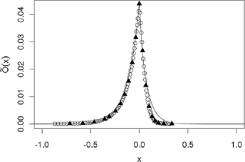
Figure 1: Observed DAX option prices (points and triangles) from 29 May 2008 with fixed maturity $T=0.314$ and different log strike prices $x$ as well as the option function generated from the estimated model (solid line).

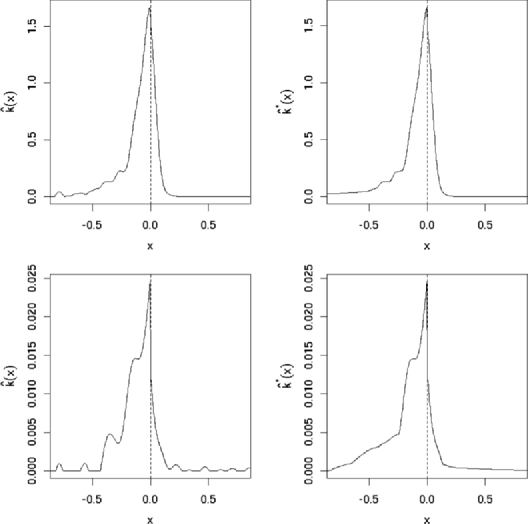
Figure 2: Using ODAX data from 29 May 2008 with three (top) and six (bottom) months to maturity, estimation of the function $k$ with (right) and without (left) rearrangement.

6 Proofs

6.1 Proof of the upper bounds

Let us recall some results of [3]: Because of the $B$-spline interpolation we obtain $\mathcal{O}_{l}(x):=\mathbb{E}[\tilde{\mathcal{O}}(x)]=\sum_{j=1}^{N}\mathcal{O}(x_{j})b_{j}(x)+\beta_{0}(x),x\in\mathbb{R}$. Furthermore, the decomposition of the stochastic error $\tilde{\psi}-\psi$ in a linearization $\mathcal{L}$ and a remainder $\mathcal{R}$,

$$\mathcal{L}(u):=T^{-1}\varphi_{T}(u-\mathrm{i})^{-1}(\mathrm{i}-u)u\mathcal{F}(\tilde{\mathcal{O}}-\mathcal{O})(u),\qquad\mathcal{R}(u):=\tilde{\psi}(u)-\psi(u)-\mathcal{L}(u),$$

$u\in\mathbb{R},$ has the following properties.

Proposition 6.1

(i) Under the hypothesis $\mathrm{e}^{-A}\lesssim\Delta^{2}$ we obtain $\sup_{u\in\mathbb{R}}|\mathbb{E}[\mathcal{F}\tilde{\mathcal{O}}(u)-\mathcal{FO}(u)]|=\sup_{u\in\mathbb{R}}|\mathcal{FO}_{l}(u)-\mathcal{FO}(u)|\lesssim\Delta^{2}$ uniformly over all Lévy triplets satisfying Assumption 1. (

• ii)]

• If the function $\kappa\colon\ \mathbb{R}\to\mathbb{R}_{+}$ satisfies (15), then for all $u\in\mathbb{R}$ the remainder is bounded by $|\mathcal{R}(u)|\leq T^{-1}\kappa(u)^{-2}(u^{4}+u^{2})|\mathcal{F}(\tilde{\mathcal{O}}-\mathcal{O})(u)|^{2}$.

Upper bound for $\gamma$ and $\alpha_{j}$ (Theorem 3.2)

Since Theorem 3.2 can be proven analogously to Theorem 4.2 in [3], we only sketch the main steps. Note that in $\mathcal{G}_{s}(R,\bar{\alpha})$ we can bound uniformly $|u^{s-1}\rho(u)|$ in representation (9), cf. Lemma 9 in [27]. Let us consider $\gamma$ first. The definition of $\hat{\gamma}$ and $w_{\gamma}^{U}$, the decomposition of $\tilde{\psi}$ and representation (9) yield

$$\hat{\gamma}=\int_{-U}^{U}\operatorname{Im}\bigl{(}\tilde{\psi}(u)\bigr{)}w_{\gamma}^{U}(u)\,\mathrm{d}u=\gamma+\int_{-U}^{U}\operatorname{Im}\bigl{(}\rho(u)+\mathcal{L}(u)+\mathcal{R}(u)\bigr{)}w_{\gamma}^{U}(u)\,\mathrm{d}u.$$

Hence, we obtain

$$\mathbb{E}\bigl{[}|\hat{\gamma}-\gamma|^{2}\bigr{]} \leq 3\biggl{|}\int_{-U}^{U}\rho(u)w_{\gamma}^{U}(u)\,\mathrm{d}u\biggr{|}^{2}+3\mathbb{E}\biggl{[}\biggl{|}\int_{-U}^{U}\mathcal{L}(u)w_{\gamma}^{U}(u)\,\mathrm{d}u\biggr{|}^{2}\biggr{]}$$

$${}+3\mathbb{E}\biggl{[}\biggl{|}\int_{-U}^{U}\mathcal{R}(u)w_{\gamma}^{U}(u)\,\mathrm{d}u\biggr{|}^{2}\biggr{]},$$

where all three summands can be estimated separately. The first one is a deterministic error term. It can be estimated using the decay of $\rho(u)$ and the weight function property (13):

$$\biggl{|}\int_{-U}^{U}\rho(u)w_{\gamma}^{U}(u)\,\mathrm{d}u\biggr{|}\lesssim\int_{-U}^{U}U^{-(s+1)}\bigl{|}\rho(u)u^{s-1}\bigr{|}\,\mathrm{d}u\lesssim U^{-s}.$$

A bias-variance decomposition, with the definition $\operatorname{Var}(Z):=\mathbb{E}[|Z-\mathbb{E}[Z]|^{2}]$, of the linear error term yields

$$\mathbb{E}\biggl{[}\biggl{|}\int_{-U}^{U}\mathcal{L}(u)w_{\gamma}^{U}(u)\,\mathrm{d}u\biggr{|}^{2}\biggr{]}$$

$$\quad=\biggl{|}\int_{-U}^{U}\frac{(\mathrm{i}-u)u}{T\varphi_{T}(u-\mathrm{i})}\mathbb{E}\bigl{[}\mathcal{F}(\tilde{\mathcal{O}}-\mathcal{O})(u)\bigr{]}w_{\gamma}^{U}(u)\,\mathrm{d}u\biggr{|}^{2}$$

$$\qquad{}+\operatorname{Var}\biggl{(}\int_{-U}^{U}\frac{(\mathrm{i}-u)u}{T\varphi_{T}(u-\mathrm{i})}\mathcal{F}\tilde{\mathcal{O}}(u)w_{\gamma}^{U}(u)\,\mathrm{d}u\biggr{)}=:\mathcal{L}_{b}^{2}+\mathcal{L}_{v}.$$

Using the approximation result in Proposition 6.1, the bound of $|\varphi_{T}(u-\mathrm{i})|^{-1}$ given by $\kappa^{-1}$ and property (13), we infer the estimate of the bias term

$$|\mathcal{L}_{b}|\lesssim\Delta^{2}U^{-(s+1)}\int_{-U}^{U}\bigl{|}\varphi_{T}(u-\mathrm{i})\bigr{|}^{-1}|u|^{s+1}\,\mathrm{d}u\lesssim\Delta^{2}U^{T\bar{\alpha}+1}.$$

For the variance part, we make use of the properties of the linear spline functions $b_{k}$ as well as $\operatorname{supp}(w_{\gamma}^{U})\subseteq[-U,U]$ and the independence of $(\varepsilon_{k})$. We estimate ($\operatorname{Cov}(Y,Z):=\mathbb{E}[(Y-\mathbb{E}[Y])\overline{(Z-\mathbb{E}[Z])}]$)

$$\mathcal{L}_{v} = \int_{-U}^{U}\int_{-U}^{U}\operatorname{Cov}\biggl{(}\frac{(\mathrm{i}-u)u}{T\varphi_{T}(u-\mathrm{i})}\mathcal{F}\tilde{\mathcal{O}}(u),\frac{(\mathrm{i}-v)v}{T\varphi_{T}(v-\mathrm{i})}\mathcal{F}\tilde{\mathcal{O}}(v)\biggr{)}w_{\gamma}^{U}(u)w_{\gamma}^{U}(v)\,\mathrm{d}u\,\mathrm{d}v$$

$$= \sum_{k=1}^{N}\delta_{k}^{2}\biggl{|}\int_{-U}^{U}\frac{(\mathrm{i}-u)u}{T\varphi_{T}(u-\mathrm{i})}\mathcal{F}b_{k}(u)w_{\gamma}^{U}(u)\,\mathrm{d}u\biggr{|}^{2}\lesssim\Delta\|\delta\|_{l^{\infty}}^{2}U^{2T\bar{\alpha}+1}.$$

To estimate the remaining term $\mathcal{R}$, we use Proposition 6.1, the property (13) of $w_{\gamma}^{U}$ and the choice of $\kappa$. In addition the independence of $(\varepsilon_{k})$ and the uniform bound of their fourth moments comes into play.

$$\mathbb{E}\biggl{[}\biggl{|}\int_{-U}^{U}\mathcal{R}(u)w_{\gamma}^{U}(u)\,\mathrm{d}u\biggr{|}^{2}\biggr{]}$$

$$\quad\lesssim\int_{-U}^{U}\int_{-U}^{U}\bigl{(}\bigl{\|}\mathcal{F}(\mathcal{O}_{l}-\mathcal{O})\bigr{\|}_{\infty}^{4}+\mathbb{E}\bigl{[}\bigl{|}\mathcal{F}(\tilde{\mathcal{O}}-\mathcal{O}_{l})(u)\mathcal{F}(\tilde{\mathcal{O}}-\mathcal{O}_{l})(v)\bigr{|}^{2}\bigr{]}\bigr{)}$$

$$\hskip 56.0pt{}\times\frac{u^{4}w_{\gamma}^{U}(u)v^{4}w_{\gamma}^{U}(v)}{\kappa(u)^{2}\kappa(v)^{2}}\,\mathrm{d}u\,\mathrm{d}v$$

$$\quad\lesssim\biggl{(}\Delta^{4}\int_{-U}^{U}\frac{u^{4}w_{\gamma}^{U}(u)}{\kappa(u)^{2}}\,\mathrm{d}u\biggr{)}^{2}+\Biggl{(}\int_{-U}^{U}\sum_{k=1}^{N}\delta_{k}^{2}\bigl{|}\mathcal{F}b_{k}(u)\bigr{|}^{2}\frac{u^{4}w_{\gamma}^{U}(u)}{\kappa(u)^{2}}\,\mathrm{d}u\Biggr{)}^{2}$$

$$\quad\lesssim\biggl{(}\Delta^{4}U^{-(s+1)}\int_{-U}^{U}\kappa(u)^{-2}|u|^{s+3}\,\mathrm{d}u\biggr{)}^{2}+\biggl{(}\Delta^{2}\|\delta\|_{l^{2}}^{2}U^{-(s+1)}\int_{-U}^{U}\kappa(u)^{-2}|u|^{s+3}\,\mathrm{d}u\biggr{)}^{2}$$

$$\quad\lesssim U^{4T\bar{\alpha}+6}\bigl{(}\Delta^{8}+\Delta^{4}\|\delta\|_{l^{2}}^{4}\bigr{)}.$$

Therefore, the total risk of $\hat{\gamma}$ is of order

$$\mathbb{E}\bigl{[}|\hat{\gamma}-\gamma|^{2}\bigr{]}\lesssim U^{-2s}+U^{2T\bar{\alpha}+1}\bigl{(}\Delta^{4}U+\Delta\|\delta\|_{l^{\infty}}^{2}\bigr{)}+U^{4T\bar{\alpha}+6}\bigl{(}\Delta^{8}+\Delta^{4}\|\delta\|_{l^{2}}^{4}\bigr{)}$$

uniformly over $\mathcal{G}_{s}(R,\bar{\alpha})$. Since the explicit choice of $U=U_{\bar{\alpha}}=\varepsilon^{-2/(2s+2T\bar{\alpha}+1)}$ fulfills $U\lesssim\Delta^{-1}$ and $\Delta\|\delta\|_{l^{2}}^{2}\lesssim\|\delta\|_{l^{\infty}}^{2}$ holds by assumption, this bound simplifies to

$$\mathbb{E}\bigl{[}|\hat{\gamma}-\gamma|^{2}\bigr{]}\lesssim U^{-2s}+U^{2T\bar{\alpha}+1}\varepsilon^{2}+U^{4T\bar{\alpha}+6}\varepsilon^{4}.$$

Here $U_{\bar{\alpha}}$ balances the trade-off between the first and the second term whereby the third term is asymptotically negligible. We obtain the claimed rate.

For $\alpha_{j},j=0,\ldots,s-2,$ the only difference to the analysis for $\hat{\gamma}$ is the rescaling factor of $w_{\alpha_{j}}^{U}$ in (13). Since its square appears in front of every term, we verify

$$\mathbb{E}\bigl{[}|\hat{\alpha}_{j}-\alpha_{j}|^{2}\bigr{]} \lesssim U^{-2(s-1-j)}+U^{2T\bar{\alpha}+2j+3}\bigl{(}\Delta^{4}U+\Delta\|\delta\|_{l^{\infty}}^{2}\bigr{)}+U^{4T\bar{\alpha}+2j+8}\bigl{(}\Delta^{8}+\Delta^{4}\|\delta\|_{l^{2}}^{4}\bigr{)}$$

$$\lesssim U^{-2(s-1-j)}+U^{2T\bar{\alpha}+2j+3}\varepsilon^{2}+U^{4T\bar{\alpha}+2j+8}\varepsilon^{4}.$$

Upper bound for $k_{e}$ (Theorem 3.4)

Similarly to the uniform bound of the bias of $\mathcal{F}\tilde{\mathcal{O}}$ in Proposition 6.1, the following lemma holds true. It can be proved analogously to Proposition 1 in [3] and thus we omit the details.

Lemma 6.2

Assuming $Ae^{-A}\lesssim\Delta^{2}$, we obtain $\sup_{u\in\mathbb{R}}|\mathbb{E}[\mathcal{F}(x(\tilde{\mathcal{O}}-\mathcal{O})(x))(u)]|=\sup_{u\in\mathbb{R}}|\mathcal{F}(x(\mathcal{O}_{l}-\mathcal{O})(x))(u)|\lesssim\Delta^{2}$ uniformly over all Lévy triplets satisfying Assumption 1 and $\mathbb{E}[|X_{T}e^{X_{T}}|]\lesssim 1$.

For convenience, we write $m:=2s-1$ and $w_{k}:=\mathcal{F}W_{k}$ such that $w_{k}(u/U)=U\times\mathcal{F}(W_{k}(Ux))(u)$. Using $\|f\|_{L^{2}}^{2}=\int_{\mathbb{R}_{+}}|f(x)|^{2}\,\mathrm{d}x+\int_{\mathbb{R}_{-}}|f(x)|^{2}\,\mathrm{d}x=:\|f\|_{L^{2}(\mathbb{R}_{+})}^{2}+\|f\|_{L^{2}(\mathbb{R}_{-})}^{2}$ for $f\in L^{2}(\mathbb{R})$, it is sufficient to consider the loss of $\hat{k}_{e}$ on $\mathbb{R}_{+}$. On $\mathbb{R}_{-}$ one can proceed analogously. We split the risk into a deterministic error, an error caused by $\hat{\gamma}$ and a stochastic error,

$$\mathbb{E}_{\mathcal{P}}\bigl{[}\|\hat{k}_{e}-k_{e}\|_{L^{2}(\mathbb{R}_{+})}^{2}\bigr{]}$$

$$\quad=\mathbb{E}_{\mathcal{P}}\biggl{[}\biggl{\|}\mathcal{F}^{-1}\biggl{(}\bigl{(}-\hat{\gamma}-\mathrm{i}\tilde{\psi}^{\prime}(u)\bigr{)}w_{k}\biggl{(}\frac{u}{U}\biggr{)}\biggr{)}-k_{e}\biggr{\|}_{L^{2}(\mathbb{R}_{+})}^{2}\biggr{]}$$

$$\quad\leq\mathbb{E}_{\mathcal{P}}\biggl{[}\int_{\mathbb{R}_{+}}3\biggl{|}\mathcal{F}^{-1}\biggl{(}\bigl{(}-\gamma-\mathrm{i}\psi^{\prime}(u)\bigr{)}w_{k}\biggl{(}\frac{u}{U}\biggr{)}\biggr{)}(x)-k_{e}(x)\biggr{|}^{2}$$

$$\hskip 36.0pt\qquad{}+3\biggl{|}\mathcal{F}^{-1}\biggl{(}(\gamma-\hat{\gamma})w_{k}\biggl{(}\frac{u}{U}\biggr{)}\biggr{)}(x)\biggr{|}^{2}$$

$$\hskip 36.0pt\qquad{}+3\biggl{|}\mathcal{F}^{-1}\biggl{(}\bigl{(}-\mathrm{i}\tilde{\psi}^{\prime}(u)+\mathrm{i}\psi^{\prime}(u)\bigr{)}w_{k}\biggl{(}\frac{u}{U}\biggr{)}\biggr{)}(x)\biggr{|}^{2}\,\mathrm{d}x\biggr{]}$$

$$\quad\leq 3\int_{\mathbb{R}_{+}}\biggl{|}\mathcal{F}^{-1}\biggl{(}\mathcal{F}k_{e}(u)w_{k}\biggl{(}\frac{u}{U}\biggr{)}\biggr{)}(x)-k_{e}(x)\biggr{|}^{2}\,\mathrm{d}x$$

$$\qquad{}+3\mathbb{E}\bigl{[}|\hat{\gamma}-\gamma|^{2}\bigr{]}\int_{\mathbb{R}_{+}}\bigl{|}UW_{k}(Ux)\bigr{|}^{2}\,\mathrm{d}x$$

$$\qquad{}+3\mathbb{E}\biggl{[}\int_{\mathbb{R}_{+}}\biggl{|}\mathcal{F}^{-1}\biggl{(}\bigl{(}\tilde{\psi}^{\prime}(u)-\psi^{\prime}(u)\bigr{)}w_{k}\biggl{(}\frac{u}{U}\biggr{)}\biggr{)}(x)\biggr{|}^{2}\,\mathrm{d}x\biggr{]}$$

$$\quad=:D+G+S.$$

The support of $W_{k}$ yields $G=0$. The deterministic term $D$ can be estimated in the spatial domain, where we use the local smoothness of $k_{e}$. For pointwise convergence rates, this was done in [2]. We decompose using $\operatorname{supp}W_{k}\subset(-\infty,0]$

$$D = 3\int_{\mathbb{R}_{+}}\bigl{|}U\bigl{(}k_{e}\ast W_{k}(U\bullet)\bigr{)}(x)-k_{e}(x)\bigr{|}^{2}\,\mathrm{d}x$$

$$\leq 6\int_{\mathbb{R}_{+}}\biggl{|}\int_{U}^{\infty}\bigl{(}k_{e}(x+y/U)-k_{e}(x)\bigr{)}W_{k}(-y)\,\mathrm{d}y\biggr{|}^{2}\,\mathrm{d}x$$

$${}+6\int_{\mathbb{R}_{+}}\biggl{|}\int_{0}^{U}\bigl{(}k_{e}(x+y/U)-k_{e}(x)\bigr{)}W_{k}(-y)\,\mathrm{d}y\biggr{|}^{2}\,\mathrm{d}x$$

$$=: 6(D_{1}+D_{2}).$$

Cauchy–Schwarz’s inequality, the estimate $\int_{U}^{\infty}|W_{k}(-y)|\,\mathrm{d}y\leq U^{-m}\int_{\mathbb{R}}|y^{m}W_{k}(y)|\,\mathrm{d}y\lesssim U^{-m}$ and Fubini’s theorem yield

$$D_{1} \leq \int_{\mathbb{R}_{+}}\int_{U}^{\infty}\bigl{|}W_{k}(-y)\bigr{|}\,\mathrm{d}y\int_{U}^{\infty}\bigl{|}k_{e}(x+y/U)-k_{e}(x)\bigr{|}^{2}\bigl{|}W_{k}(-y)\bigr{|}\,\mathrm{d}y\,\mathrm{d}x$$

$$\lesssim U^{-m}\int_{\mathbb{R}_{+}}\int_{U}^{\infty}\bigl{(}\bigl{|}k_{e}(x+y/U)\bigr{|}^{2}+\bigl{|}k_{e}(x)\bigr{|}^{2}\bigr{)}\bigl{|}W_{k}(-y)\bigr{|}\,\mathrm{d}y\,\mathrm{d}x$$

$$\lesssim U^{-m}\int_{U}^{\infty}\bigl{|}W_{k}(-y)\bigr{|}\int_{\mathbb{R}_{+}}\bigl{|}k_{e}(x+y/U)\bigr{|}^{2}+\bigl{|}k_{e}(x)\bigr{|}^{2}\,\mathrm{d}x\,\mathrm{d}y\lesssim U^{-2m}\|k_{e}\|_{L^{2}}^{2}.$$

Using a Taylor expansion, we split $D_{2}$ in a polynomial part and a remainder:

$$D_{2} \leq 2\int_{\mathbb{R}_{+}}\Biggl{|}\int_{0}^{U}\Biggl{(}\sum_{j=0}^{s-1}\frac{k_{e}^{(j)}(x)}{j!U^{j}}y^{j}\Biggr{)}W_{k}(-y)\,\mathrm{d}y\Biggr{|}^{2}\,\mathrm{d}x$$

$${}+2\int_{\mathbb{R}_{+}}\biggl{|}\int_{0}^{U}\int_{x}^{x+{y}/{U}}\frac{k_{e}^{(s)}(z)(x+y/U-z)^{s-1}}{(s-1)!}\,\mathrm{d}zW_{k}(-y)\,\mathrm{d}y\biggr{|}^{2}\,\mathrm{d}x=:2D_{2P}+2D_{2R}.$$

We estimate by $\int_{0}^{U}y^{j}W_{k}(-y)\,\mathrm{d}y=-\int_{U}^{\infty}y^{j}W_{k}(-y)\,\mathrm{d}y$ for $j=0,\ldots,s-1$

$$D_{2P}\leq sU^{-2m}\sum_{j=0}^{s-1}\frac{1}{(j!)^{2}}\int_{\mathbb{R}_{+}}\bigl{|}k_{e}^{(j)}(x)\bigr{|}^{2}\,\mathrm{d}x\biggl{(}\int_{\mathbb{R}_{+}}\bigl{|}y^{m}W_{k}(-y)\bigr{|}\,\mathrm{d}y\biggr{)}^{2}\lesssim U^{-2m}\sum_{j=0}^{s-1}\bigl{\|}k_{e}^{(j)}\bigr{\|}_{L^{2}}^{2}.$$

With twofold usage of Cauchy–Schwarz and with Fubini’s theorem we obtain

$$D_{2R} = \int_{\mathbb{R}_{+}}\biggl{|}\int_{0}^{U}\int_{0}^{y/U}\frac{k_{e}^{(s)}(x+z)(y/U-z)^{s-1}}{(s-1)!}\,\mathrm{d}zW_{k}(-y)\,\mathrm{d}y\biggr{|}^{2}\,\mathrm{d}x$$

$$\leq \int_{\mathbb{R}_{+}}\biggl{(}\int_{0}^{U}\biggl{(}\int_{0}^{{y}/{U}}\bigl{|}k_{e}^{(s)}(x+z)\bigr{|}^{2}\,\mathrm{d}z\biggr{)}^{1/2}$$

$$\hskip 41.0pt{}\times\biggl{(}\int_{0}^{{y}/{U}}\frac{({y}/{U}-z)^{2s-2}}{((s-1)!)^{2}}\,\mathrm{d}z\biggr{)}^{1/2}\bigl{|}W_{k}(-y)\bigr{|}\,\mathrm{d}y\biggr{)}^{2}\,\mathrm{d}x$$

$$\leq \int_{\mathbb{R}_{+}}\int_{0}^{U}\int_{0}^{{y}/{U}}\bigl{|}k_{e}^{(s)}(x+z)\bigr{|}^{2}\,\mathrm{d}z\bigl{|}W_{k}(-y)\bigr{|}\,\mathrm{d}y\int_{0}^{U}\frac{(y/U)^{2s-1}}{(2s-1)((s-1)!)^{2}}\bigl{|}W_{k}(-y)\bigr{|}\,\mathrm{d}y\,\mathrm{d}x$$

$$\lesssim U^{-(2s-1)}\int_{0}^{U}\int_{0}^{y/U}\int_{\mathbb{R}_{+}}\bigl{|}k_{e}^{(s)}(x+z)\bigr{|}^{2}\,\mathrm{d}x\,\mathrm{d}z\bigl{|}W_{k}(-y)\bigr{|}\,\mathrm{d}y$$

$$\leq U^{-(2s-1)}\bigl{\|}k_{e}^{(s)}\bigr{\|}_{L^{2}}^{2}\int_{0}^{U}\frac{y}{U}\bigl{|}W_{k}(-y)\bigr{|}\,\mathrm{d}y\lesssim U^{-2s}.$$

Therefore, we have $D+G\lesssim U^{-2s}+U\mathbb{E}[|\hat{\gamma}-\gamma|^{2}]$.

To estimate the stochastic error $S$, we bound the term $|\tilde{\psi}^{\prime}(u)-\psi^{\prime}(u)|$. Let us introduce the notation

$$\tilde{\varphi}_{T}(u-\mathrm{i}) := v_{\kappa(u)}\bigl{(}1+\bigl{(}\mathrm{i}u-u^{2}\bigr{)}\mathcal{F}\tilde{\mathcal{O}}(u)\bigr{)},$$

$$\tilde{\varphi}^{\prime}_{T}(u-\mathrm{i}) := (\mathrm{i}-2u)\mathcal{F}\tilde{\mathcal{O}}(u)-\bigl{(}u+\mathrm{i}u^{2}\bigr{)}\mathcal{F}\bigl{(}x\tilde{\mathcal{O}}(x)\bigr{)}(u),\qquad u\in\mathbb{R}.$$

For all $u\in\mathbb{R}$ where $|\tilde{\varphi}_{T}(u-\mathrm{i})|>\kappa(u)$ we obtain $\tilde{\varphi}_{T}(u-\mathrm{i})=1+(\mathrm{i}u-u^{2})\mathcal{F}\tilde{\mathcal{O}}(u)$. For $|\tilde{\varphi}_{T}(u-\mathrm{i})|=\kappa(u)$ the estimate $|\tilde{\varphi}_{T}(u-\mathrm{i})-\varphi_{T}(u-\mathrm{i})|\geq 2\kappa(u)$ follows from (15). This yields

$$\bigl{|}\tilde{\varphi}_{T}(u-\mathrm{i})-\varphi_{T}(u-\mathrm{i})\bigr{|} \leq \bigl{|}1+\bigl{(}\mathrm{i}u-u^{2}\bigr{)}\mathcal{F}\tilde{\mathcal{O}}(u)-\varphi_{T}(u-\mathrm{i})\bigr{|}+\kappa(u)$$

$$\leq \bigl{|}1+\bigl{(}\mathrm{i}u-u^{2}\bigr{)}\mathcal{F}\tilde{\mathcal{O}}(u)-\varphi_{T}(u-\mathrm{i})\bigr{|}+{\textstyle\frac{1}{2}}\bigl{|}\tilde{\varphi}_{T}(u-\mathrm{i})-\varphi_{T}(u-\mathrm{i})\bigr{|}.$$

Therefore, $|\tilde{\varphi}_{T}(u-\mathrm{i})-\varphi_{T}(u-\mathrm{i})|\leq 2|1+(\mathrm{i}u-u^{2})\mathcal{F}\tilde{\mathcal{O}}(u)-\varphi_{T}(u-\mathrm{i})|$ holds for all $u\in\mathbb{R}$. We obtain a similar decomposition as [15],

$$\bigl{|}\tilde{\psi}^{\prime}(u)-\psi^{\prime}(u)\bigr{|} = \frac{1}{T}\biggl{|}\frac{\tilde{\varphi}^{\prime}_{T}(u-\mathrm{i})}{\tilde{\varphi}_{T}(u-\mathrm{i})}-\frac{\varphi^{\prime}_{T}(u-\mathrm{i})}{\varphi_{T}(u-\mathrm{i})}\biggr{|}$$

$$\leq \frac{1}{T|\tilde{\varphi}_{T}(u-\mathrm{i})|}\bigl{(}\bigl{|}\tilde{\varphi}^{\prime}_{T}(u-\mathrm{i})-\varphi^{\prime}_{T}(u-\mathrm{i})\bigr{|}+T\bigl{|}\psi^{\prime}(u)\bigr{|}\bigl{|}\varphi_{T}(u-\mathrm{i})-\tilde{\varphi}_{T}(u-\mathrm{i})\bigr{|}\bigr{)}$$

$$\leq \frac{1}{2T\kappa(u)}\bigl{(}\bigl{(}\bigl{(}1+4u^{2}\bigr{)}^{1/2}+2T\bigl{|}\psi^{\prime}(u)\bigr{|}\bigl{(}u^{2}+u^{4}\bigr{)}^{1/2}\bigr{)}\bigl{|}\mathcal{F}(\tilde{\mathcal{O}}-\mathcal{O})(u)\bigr{|}$$

$$\hskip 38.0pt{}+\bigl{(}u^{2}+u^{4}\bigr{)}^{1/2}\bigl{|}\mathcal{F}\bigl{(}x(\tilde{\mathcal{O}}-\mathcal{O})(x)\bigr{)}(u)\bigr{|}\bigr{)}.$$

Since $|\psi^{\prime}(u)|\leq|\gamma|+\|k_{e}\|_{L^{1}}\leq 2R$, we have

$$\bigl{|}\tilde{\psi}^{\prime}(u)-\psi^{\prime}(u)\bigr{|}\lesssim\frac{1}{\kappa(u)}\bigl{(}\bigl{(}1+u^{2}\bigr{)}\bigl{|}\mathcal{F}(\tilde{\mathcal{O}}-\mathcal{O})(u)\bigr{|}+\bigl{(}u^{2}+u^{4}\bigr{)}^{1/2}\bigl{|}\mathcal{F}\bigl{(}x(\tilde{\mathcal{O}}-\mathcal{O})(x)\bigr{)}(u)\bigr{|}\bigr{)}.$$

It follows with Plancherel’s equality

$$S \leq 3\mathbb{E}\bigl{[}\bigl{\|}\mathcal{F}^{-1}\bigl{(}\bigl{(}\tilde{\psi}^{\prime}(u)-\psi^{\prime}(u)\bigr{)}w_{k}(u/U)\bigr{)}\bigr{\|}_{L^{2}}^{2}\bigr{]}$$

$$= \frac{3}{2\uppi}\int_{\mathbb{R}}\mathbb{E}\bigl{[}\bigl{|}\tilde{\psi}^{\prime}(u)-\psi^{\prime}(u)\bigr{|}^{2}\bigr{]}\bigl{|}w_{k}(u/U)\bigr{|}^{2}\,\mathrm{d}u$$

$$\lesssim \int_{\mathbb{R}}\frac{u^{4}}{|\kappa(u)|^{2}}\bigl{(}\mathbb{E}\bigl{[}\bigl{|}\mathcal{F}(\tilde{\mathcal{O}}-\mathcal{O})(u)\bigr{|}^{2}\bigr{]}$$

$$\hskip 37.0pt\quad{}+\mathbb{E}\bigl{[}\bigl{|}\mathcal{F}\bigl{(}x(\tilde{\mathcal{O}}-\mathcal{O})(x)\bigr{)}(u)\bigr{|}^{2}\bigr{]}\bigr{)}\bigl{|}w_{k}(u/U)\bigr{|}^{2}\,\mathrm{d}u$$

$$=: S_{1}+S_{2}.$$

Both terms can be estimated similarly. Thus, we only write it down for $S_{2}$, where stronger conditions are needed. Lemma 6.2 and $\|\mathcal{F}(xb_{j}(x))\|_{\infty}\leq 2\Delta(x_{j}+\Delta)$, $j=1,\ldots,N$, yield

$$S_{2} \leq \int_{\mathbb{R}}\frac{u^{4}}{|\kappa(u)|^{2}}\bigl{(}\bigl{\|}x(O_{l}-O)(x)\bigr{\|}_{\infty}^{2}+\operatorname{Var}\bigl{(}\mathcal{F}\bigl{(}x\tilde{\mathcal{O}}(x)\bigr{)}(u)\bigr{)}\bigr{)}\bigl{|}w_{k}(u/U)\bigr{|}^{2}\,\mathrm{d}u$$

$$\lesssim \int_{\mathbb{R}}|u|^{2T\bar{\alpha}+4}\Biggl{(}\Delta^{4}+\sum_{j=1}^{N}\delta_{j}^{2}\bigl{|}\mathcal{F}\bigl{(}xb_{j}(x)\bigr{)}(u)\bigr{|}^{2}\Biggr{)}\bigl{|}w_{k}(u/U)\bigr{|}^{2}\,\mathrm{d}u$$

$$\lesssim \bigl{(}\Delta^{4}+\Delta^{2}\bigl{\|}(x_{j}\delta_{j})\bigr{\|}_{l^{2}}^{2}+\Delta^{4}\|\delta_{j}\|_{l^{2}}^{2}\bigr{)}U^{2T\bar{\alpha}+5}\lesssim\varepsilon^{2}U^{2T\bar{\alpha}+5}.$$

Therefore, we have shown $\mathbb{E}[\|\hat{k}_{e}-k_{e}\|_{L^{2},\tau}^{2}]\lesssim U^{-2s}+\varepsilon^{2}U^{2T\bar{\alpha}+5}+U\mathbb{E}[|\hat{\gamma}-\gamma|^{2}]$. The assertion follows from the asymptotic optimal choice $U=U_{\bar{\alpha}}=\varepsilon^{-2/(2s+2T\bar{\alpha}+5)}$ and the assumption on the risk of $\hat{\gamma}$.

6.2 Proof of Proposition 4.1

Step 1: Let $(a_{\varepsilon})_{\varepsilon>0}$ be a deterministic sequence such that there is a constant $C>0$ with $|a_{\varepsilon}-\alpha|\leq C|\log\varepsilon|^{-1}$. Let the estimator $\hat{\alpha}_{0}$ use the cut-off value $U_{\varepsilon}:=\tilde{U}_{a_{\varepsilon}}$ and the trimming parameter $\kappa_{\varepsilon}:=\tilde{\kappa}_{\bar{a}_{\varepsilon}}$, with $\bar{a}_{\varepsilon}:=a_{\varepsilon}+C|\log\varepsilon|^{-1}$, as defined in (16) and (17). Then we can show the asymptotic risk bound $\sup_{\mathcal{P}\in\mathcal{G}_{s}(R,\alpha)}\mathbb{E}_{\mathcal{P}}[|\hat{\alpha}_{0}-\alpha|^{2}]^{1/2}\lesssim\varepsilon^{2(s-1)/(2s+2T\alpha+1)}$ as follows: By construction holds $\alpha\leq\bar{a}_{\varepsilon}$. Hence, $\kappa_{\varepsilon}$ fulfills condition (15) for each pair $\mathcal{P}\in\mathcal{G}_{s}(R,\alpha)$ and thus we deduce from Theorem 3.2

$$\mathbb{E}_{\mathcal{P}}\bigl{[}\bigl{|}\hat{\alpha}_{0}-\alpha\bigr{|}^{2}\bigr{]}$$

$$\quad\lesssim U_{\varepsilon}^{-2(s-1)}+U_{\varepsilon}^{2T\alpha+3}\varepsilon^{2}+U_{\varepsilon}^{4T\bar{a}_{\varepsilon}+8}\varepsilon^{4}$$ (21)

$$\quad=\varepsilon^{4(s-1)/(2s+2Ta_{\varepsilon}+1)}\bigl{(}1+\varepsilon^{4T(a_{\varepsilon}-\alpha)/(2s+2Ta_{\varepsilon}+1)}+\varepsilon^{(4s-8+8T(a_{\varepsilon}-\bar{a}_{\varepsilon}))/(2s+2Ta_{\varepsilon}+1)}\bigr{)}.$$

The first factor has the claimed order, since $\varepsilon^{4(s-1)/(2s+2Ta_{\varepsilon}+1)}\lesssim\varepsilon^{4(s-1)/(2s+2T\alpha+1)}$ follows with easy calculations from $(\alpha-a_{\varepsilon})\log\varepsilon\leq C$. Hence, the claim follows once we have bound the sum in the bracket of equation (6.2). For the second term, this is implied by

$$\biggl{|}\frac{4T(a_{\varepsilon}-\alpha)}{2s+2Ta_{\varepsilon}+1}\log\varepsilon\biggr{|}\leq\frac{4T|(a_{\varepsilon}-\alpha)\log\varepsilon|}{2s+1}\leq\frac{4TC}{2s+1}.$$

To estimate the third term, we obtain from $s\geq 2$ and $\varepsilon<1$

$$\frac{4s-8+8T(a_{\varepsilon}-\bar{a}_{\varepsilon})}{2s+2Ta_{\varepsilon}+1}\log\varepsilon\leq\frac{-8TC|\log\varepsilon|^{-1}}{2s+1}\log\varepsilon\leq\frac{8TC}{2s+1}.$$

Step 2: Let $\mathcal{P}\in\mathcal{G}_{s}(R,\alpha)$. Note that $\kappa_{\varepsilon}$ satisfies the condition (15) on the set $\{|\hat{\alpha}_{\mathrm{pre}}-\alpha|<|\log\varepsilon|^{-1}\}$. Using the independence of $\hat{\alpha}_{\mathrm{pre}}$ and $O_{j}$, the almost sure bound $\tilde{\alpha}_{0}\leq\bar{\alpha}$ and the concentration of $\hat{\alpha}_{\mathrm{pre}}$, we deduce from step 1:

$$\mathbb{E}_{\mathcal{P},\hat{\alpha}_{\mathrm{pre}}}\bigl{[}\bigl{|}\tilde{\alpha}_{0}-\alpha\bigr{|}^{2}\bigr{]} \leq \mathbb{E}_{\mathcal{P},\hat{\alpha}_{\mathrm{pre}}}\bigl{[}\mathbb{E}_{\mathcal{P},\hat{\alpha}_{\mathrm{pre}}}\bigl{[}|\tilde{\alpha}_{0}-\alpha|^{2}|\hat{\alpha}_{\mathrm{pre}}\bigr{]}\mathbf{1}_{\{|\hat{\alpha}_{\mathrm{pre}}-\alpha|<|\log\varepsilon|^{-1}\}}\bigr{]}$$

$${}+4\bar{\alpha}^{2}\mathbb{P}_{\hat{\alpha}_{\mathrm{pre}}}\bigl{(}|\hat{\alpha}_{\mathrm{pre}}-\alpha|\geq|\log\varepsilon|^{-1}\bigr{)}$$

$$\lesssim \varepsilon^{4(s-1)/(2s+2T\alpha+1)}+4\bar{\alpha}^{2}{d}\varepsilon^{2}.$$

Since the second term decreases faster then the first one for $\varepsilon\to 0$, we obtain the claimed rate.

6.3 Proof of Proposition 4.2

Recall that the cut-off value of $\hat{\alpha}_{0}$ is given by $U=\varepsilon^{-2/(2s+2T\bar{\alpha}+1)}$. For $\kappa>0,$ we obtain from the definition of the estimator and the decomposition of the stochastic error into linear part and remainder:

$$\mathbb{P}\bigl{(}|\hat{\alpha}_{0}-\alpha|\geq\kappa\bigr{)} = \mathbb{P}\biggl{(}\biggl{|}\int_{-U}^{U}\operatorname{Re}(\rho+\tilde{\psi}-\psi)(u)w_{\alpha_{0}}^{U}(u)\,\mathrm{d}u\biggr{|}\geq\kappa\biggr{)}$$

$$\leq \mathbb{P}\biggl{(}\biggl{|}\int_{-U}^{U}\rho(u)w_{\alpha_{0}}^{U}(u)\,\mathrm{d}u\biggr{|}\geq\frac{\kappa}{3}\biggr{)}+\mathbb{P}\biggl{(}\biggl{|}\int_{-U}^{U}\operatorname{Re}\bigl{(}\mathcal{L}(u)\bigr{)}w_{\alpha_{0}}^{U}(u)\,\mathrm{d}u\biggr{|}\geq\frac{\kappa}{3}\biggr{)}$$

$${}+\mathbb{P}\biggl{(}\biggl{|}\int_{-U}^{U}\mathcal{R}(u)w_{\alpha_{0}}^{U}(u)\,\mathrm{d}u\biggr{|}\geq\frac{\kappa}{3}\biggr{)}=:P_{1}+P_{2}+P_{3}.$$

We will bound all three probabilities separately. To that end, let $c_{j},j\in\mathbb{N},$ be suitable non-negative constants not depending on $\kappa,\varepsilon$ and $N$.

The event in $P_{1}$ is deterministic. Hence, the same estimate on the deterministic error as in Theorem 3.2

$$\biggl{|}\int_{-U}^{U}\rho(u)w_{\alpha_{0}}^{U}(u)\,\mathrm{d}u\biggr{|}\leq c_{1}U^{-(s-1)}=c_{1}\varepsilon^{2(s-1)/(2s+2T\bar{\alpha}+1)}$$

yields $P_{1}=0$ for all $\varepsilon<\varepsilon^{(1)}:=(\kappa/(3c_{1}))^{(2s+2T\bar{\alpha}+1)/(2s-2)}$.

To bound $P_{2}$ we infer from the definition of $\mathcal{L}$, the linearity of the errors in $\tilde{\mathcal{O}}=\mathcal{O}_{l}+\sum_{j=1}^{N}\delta_{j}\varepsilon_{j}bj$ and from the estimate of the term $|\mathcal{L}_{b}|$ in Theorem 3.2

$$\biggl{|}\int_{-U}^{U}\operatorname{Re}\bigl{(}\mathcal{L}(u)\bigr{)}w_{\alpha_{0}}^{U}(u)\,\mathrm{d}u\biggr{|}$$

$$\quad=\biggl{|}\int_{-U}^{U}\operatorname{Re}\biggl{(}\frac{(\mathrm{i}-u)u}{T\varphi_{T}(u-\mathrm{i})}\mathcal{F}(\tilde{\mathcal{O}}-\mathcal{O})(u)\biggr{)}w_{\alpha_{0}}^{U}(u)\,\mathrm{d}u\biggr{|}$$

$$\quad\leq\int_{-U}^{U}\frac{(u^{4}+u^{2})^{1/2}}{T|\varphi_{T}(u-\mathrm{i})|}\bigl{|}\mathcal{F(O}_{l}-\mathcal{O})(u)w_{\alpha_{0}}^{U}(u)\bigr{|}\,\mathrm{d}u$$

$$\qquad{}+\biggl{|}\int_{-U}^{U}\operatorname{Re}\Biggl{(}\frac{(\mathrm{i}-u)u}{T\varphi_{T}(u-\mathrm{i})}\sum_{j=1}^{N}\delta_{j}\varepsilon_{j}\mathcal{F}b_{j}(u)\Biggr{)}w_{\alpha_{0}}^{U}(u)\,\mathrm{d}u\biggr{|}$$

$$\quad\leq c_{2}\Delta^{2}U^{T\bar{\alpha}+2}+\Biggl{|}\sum_{j=1}^{N}\delta_{j}\varepsilon_{j}\int_{-U}^{U}\operatorname{Re}\biggl{(}\frac{(\mathrm{i}-u)u}{T\varphi_{T}(u-\mathrm{i})}\mathcal{F}b_{j}(u)\biggr{)}w_{\alpha_{0}}^{U}(u)\,\mathrm{d}u\Biggr{|}$$

$$\quad\leq c_{2}\varepsilon^{2(s-1)/(2s+2T\bar{\alpha}+1)}+\Biggl{|}\sum_{j=1}^{N}a_{j}\varepsilon_{j}\Biggr{|},$$

where the coefficients are given by $a_{j}:=\delta_{j}\int_{-U}^{U}\operatorname{Re}(\frac{(\mathrm{i}-u)u}{T\varphi_{T}(u-\mathrm{i})}\mathcal{F}b_{j}(u))w_{\alpha_{0}}^{U}(u)\,\mathrm{d}u$ for $j=1,\ldots,N$. To apply (19), we deduce from $\|\mathcal{F}b_{j}\|_{\infty}\leq 2\Delta$, the weight function property (13) and the assumption $\Delta\|\delta\|_{l^{2}}^{2}\lesssim\|\delta\|_{l^{\infty}}^{2}$

$$\sum_{j=1}^{N}a_{j}^{2} \leq \sum_{j=1}^{N}\delta_{j}^{2}\biggl{(}\int_{-U}^{U}\frac{(u^{4}+u^{2})^{1/2}}{T|\varphi_{T}(u-\mathrm{i})|}\bigl{|}\mathcal{F}b_{j}(u)\bigr{|}\bigl{|}w_{\alpha_{0}}^{U}(u)\bigr{|}\,\mathrm{d}u\biggr{)}^{2}\leq c_{3}\Delta^{2}U^{2T\bar{\alpha}+4}\|\delta\|_{l^{2}}^{2}$$

$$\leq c_{4}\varepsilon^{2}U^{2T\bar{\alpha}+4}=c_{4}\varepsilon^{2(s-1)/(2s+2T\bar{\alpha}+1)}.$$

This implies through the concentration inequality of $(\varepsilon_{j})$

$$P_{2} \leq \mathbb{P}\Biggl{(}\Biggl{|}\sum_{j=1}^{N}a_{j}\varepsilon_{j}\Biggr{|}\geq\frac{\kappa}{6}\Biggr{)}+\mathbb{P}\biggl{(}c_{2}\varepsilon^{2(s-1)/(2s+2T\bar{\alpha}+1)}\geq\frac{\kappa}{6}\biggr{)}$$

$$\leq C_{1}\exp\biggl{(}-\frac{C_{2}}{36c_{4}}\kappa^{2}\varepsilon^{-2(s-1)/(2s+2T\bar{\alpha}+1)}\biggr{)}$$

for all $\varepsilon<\varepsilon^{(2)}:=(\kappa/(6c_{2}))^{(2s+2T\bar{\alpha}+1)/(2s-2)}$.

It remains to estimate probability $P_{3}$. The bound of $\mathcal{R}$ in Proposition 6.1 ii) yields

$$\biggl{|}\int_{-U}^{U}\mathcal{R}(u)w_{\alpha_{0}}^{U}(u)\,\mathrm{d}u\biggr{|}$$

$$\quad\leq\int_{-U}^{U}\frac{u^{4}+u^{2}}{T\kappa(u)^{2}}\bigl{|}\mathcal{F}(\tilde{\mathcal{O}}-\mathcal{O})(u)\bigr{|}^{2}\bigl{|}w_{\alpha_{0}}^{U}(u)\bigr{|}\,\mathrm{d}u$$

$$\quad\leq 2\int_{-U}^{U}\frac{u^{4}+u^{2}}{T\kappa(u)^{2}}\bigl{|}\mathcal{F(O}_{l}-\mathcal{O})(u)\bigr{|}^{2}\bigl{|}w_{\alpha_{0}}^{U}(u)\bigr{|}\,\mathrm{d}u$$

$$\qquad{}+2\int_{-U}^{U}\frac{u^{4}+u^{2}}{T\kappa(u)^{2}}\Biggl{|}\sum_{j=1}^{N}\delta_{j}\varepsilon_{j}\mathcal{F}b_{j}(u)\Biggr{|}^{2}\bigl{|}w_{\alpha_{0}}^{U}(u)\bigr{|}\,\mathrm{d}u.$$

The first addend gets small owing to Proposition 6.1(i):

$$\int_{-U}^{U}\frac{u^{4}+u^{2}}{T\kappa(u)^{2}}\bigl{|}\mathcal{F(O}_{l}-\mathcal{O})(u)\bigr{|}^{2}\bigl{|}w_{\alpha_{0}}^{U}(u)\bigr{|}\,\mathrm{d}u$$

$$\quad\leq\bigl{\|}\mathcal{F(O}_{l}-\mathcal{O})\bigr{\|}_{\infty}^{2}\int_{-U}^{U}\frac{u^{4}+u^{2}}{T\kappa(u)^{2}}\bigl{|}w_{\alpha_{0}}^{U}(u)\bigr{|}\,\mathrm{d}u$$

$$\quad\leq c_{5}\Delta^{4}U^{2T\bar{\alpha}+4}\leq c_{5}\varepsilon^{2(s-1)/(2s+2T\bar{\alpha}+1)}.$$

For the second one, we obtain

$$\Biggl{|}\sum_{j=1}^{N}\delta_{j}\varepsilon_{j}\mathcal{F}b_{j}(u)\Biggr{|}^{2}=\sum_{j=1}^{N}\delta_{j}^{2}\varepsilon_{j}^{2}\bigl{|}\mathcal{F}b_{j}(u)\bigr{|}^{2}+2\sum_{j=2}^{N}\sum_{k=1}^{j-1}\delta_{j}\delta_{k}\varepsilon_{j}\varepsilon_{k}\operatorname{Re}\bigl{(}\mathcal{F}b_{j}(u)\mathcal{F}b_{k}(-u)\bigr{)}.$$

Thus,

$$\biggl{|}\int_{-U}^{U}\mathcal{R}(u)w_{\alpha_{0}}^{U}(u)\,\mathrm{d}u\biggr{|}\leq 2c_{5}\varepsilon^{{(4s-6)}/{(2s+2T\bar{\alpha}+1)}}+2\sum_{j=1}^{N}\delta_{j}^{2}\varepsilon_{j}^{2}\xi_{j,j}(U)+4\sum_{j=2}^{N}\sum_{k=1}^{j-1}\delta_{j}\delta_{k}\varepsilon_{j}\varepsilon_{k}\xi_{j,k}(U)$$

with $\xi_{j,k}(U):=\int_{-U}^{U}\frac{u^{4}+u^{2}}{T\kappa(u)^{2}}\operatorname{Re}(\mathcal{F}b_{j}(u)\mathcal{F}b_{k}(-u))|w_{\alpha_{0}}^{U}(u)|\,\mathrm{d}u$. Denoting the diagonal term and the cross term as

$$D_{N}:=\sum_{j=1}^{N}\delta_{j}^{2}\varepsilon_{j}^{2}\xi_{j,j}(U)\quad\mbox{and}\quad U_{N}:=\sum_{j=2}^{N}\sum_{k=1}^{j-1}\delta_{j}\delta_{k}\varepsilon_{j}\varepsilon_{k}\xi_{j,k}(U),$$

respectively, we obtain

$$P_{3}\leq\mathbb{P}\biggl{(}2c_{5}\varepsilon^{2(s-1)/(2s+2T\bar{\alpha}+1)}\geq\frac{\kappa}{9}\biggr{)}+\mathbb{P}\biggl{(}2D_{N}\geq\frac{\kappa}{9}\biggr{)}+\mathbb{P}\biggl{(}4U_{N}\geq\frac{\kappa}{9}\biggr{)}.$$

The first summand vanishes for $\varepsilon<\varepsilon^{(3)}:=(\kappa/(18c_{5}))^{(2s+2T\bar{\alpha}+1)/(2s-2)}$. To estimate the probabilities on $D_{N}$ and $U_{N}$, we establish the bound

$$\bigl{|}\xi_{j,k}(U)\bigr{|}\leq\|\mathcal{F}b_{j}\|_{\infty}\|\mathcal{F}b_{k}\|_{\infty}\int_{-U}^{U}\frac{u^{4}+u^{2}}{T\kappa(u)^{2}}\bigl{|}w_{\alpha_{0}}^{U}(u)\bigr{|}\,\mathrm{d}u\leq c_{6}\Delta^{2}U^{2T\bar{\alpha}+4}$$ (22)

for $j,k=1,\ldots,N$. Hence,

$$\Biggl{|}\sum_{j=1}^{N}\delta_{j}^{2}\xi_{j,j}(U)\Biggr{|}\leq c_{6}\Delta^{2}\|\delta\|_{l^{2}}^{2}U^{2T\bar{\alpha}+4}\leq c_{7}\varepsilon^{2}U^{2T\bar{\alpha}+4}\leq c_{7}\varepsilon^{2(s-1)/(2s+2T\bar{\alpha}+1)},$$

which yields together with (19)

$$\mathbb{P}\biggl{(}D_{N}\geq\frac{\kappa}{18}\biggr{)} \leq \mathbb{P}\Biggl{(}\sup_{k=1,\ldots,N}|\varepsilon_{k}|^{2}\Biggl{|}\sum_{j=1}^{N}\delta_{j}^{2}\xi_{j,j}(U)\Biggr{|}\geq\frac{\kappa}{18}\Biggr{)}$$

$$\leq \mathbb{P}\biggl{(}\sup_{k=1,\ldots,N}|\varepsilon_{k}|^{2}\geq\frac{\kappa}{18c_{7}}\varepsilon^{-2(s-1)/(2s+2T\bar{\alpha}+1)}\biggr{)}$$

$$\leq C_{1}N\exp\biggl{(}-\frac{C_{2}}{18c_{7}}\kappa\varepsilon^{-2(s-1)/(2s+2T\bar{\alpha}+1)}\biggr{)}.$$

To derive an exponential inequality for the U-statistic $U_{N}$, we apply the martingale idea in [13]. Because of the independence and the centering of the $(\varepsilon_{j})$, the process $(U_{N})_{N\geq 1}$ is a martingale with respect to its natural filtration $(\mathcal{F}_{N}^{U})$ (setting $U_{1}=0$):

$$\mathbb{E}\bigl{[}U_{N}-U_{N-1}|\mathcal{F}_{N-1}^{U}\bigr{]}=\mathbb{E}\Biggl{[}\sum_{k=1}^{N-1}\delta_{N}\delta_{k}\varepsilon_{N}\varepsilon_{k}\xi_{N,k}(U)\Big{|}\mathcal{F}_{N-1}^{U}\Biggr{]}=0.$$

We apply the martingale version of the Bernstein inequality, see Theorem VII.3.6 in [22], which yields for arbitrary $t,Q,S>0$

$$\mathbb{P}\bigl{(}|U_{N}|\geq t\bigr{)} \leq 2\mathbb{P}\bigl{(}\langle U\rangle_{N}>Q\bigr{)}+2\mathbb{P}\Bigl{(}\max_{k=1,\ldots,N}|U_{k}-U_{k-1}|>S\Bigr{)}$$

$${}+2\exp\biggl{(}-\frac{t^{2}}{4(Q+tS)}\biggr{)}.$$

Hence, we consider the increment $|U_{N}-U_{N-1}|=|\varepsilon_{N}||\sum_{k=1}^{N-1}\delta_{N}\delta_{k}\xi_{N,k}(U)\varepsilon_{k}|$, for $N\geq 2$. Denoting $a_{N,k}:=\delta_{N}\delta_{k}\xi_{N,k}(U)$, we estimate using (22)

$$\sum_{k=1}^{N-1}a_{N,k}^{2} = \delta_{N}^{2}\sum_{k=1}^{N-1}\delta_{k}^{2}\xi_{N,k}(U)^{2}\leq c_{6}^{2}\Delta^{4}U^{4T\bar{\alpha}+8}\delta_{N}^{2}\|\delta\|_{l^{2}}^{2}$$

$$\leq c_{6}^{2}\Delta^{4}\|\delta\|_{l^{2}}^{4}U^{4T\bar{\alpha}+8}\leq c_{7}^{2}\varepsilon^{4}U^{4T\bar{\alpha}+8}\leq c_{7}^{2}\varepsilon^{4(s-1)/(2s+2T\bar{\alpha}+1)}.$$

Thus, by Assumption (19) we obtain for all $S>0$

$$\mathbb{P}\bigl{(}|U_{N}-U_{N-1}|>S\bigr{)}$$

$$\quad=\mathbb{P}\Biggl{(}|\varepsilon_{N}|\Biggl{|}\sum_{k=1}^{N-1}a_{N,k}\varepsilon_{k}\Biggr{|}>S\Biggr{)}$$

$$\quad\leq\mathbb{P}\bigl{(}|\varepsilon_{N}|>\sqrt{S}\varepsilon^{-(s-1)/(2s+2T\bar{\alpha}+1)}\bigr{)}+\mathbb{P}\Biggl{(}\Biggl{|}\sum_{k=1}^{N-1}a_{N,k}\varepsilon_{k}\Biggr{|}>\sqrt{S}\varepsilon^{(s-1)/(2s+2T\bar{\alpha}+1)}\Biggr{)}$$

$$\quad\leq C_{1}\exp\bigl{(}-C_{2}S\varepsilon^{-2(s-1)/(2s+2T\bar{\alpha}+1)}\bigr{)}$$

$$\qquad{}+C_{1}\exp\biggl{(}-\frac{C_{2}}{c_{7}^{2}}S\varepsilon^{-2(s-1)/(2s+2T\bar{\alpha}+1)}\biggr{)}.$$

The quadratic variation of $U_{N}$ is given by

$$\langle U\rangle_{N}-\langle U\rangle_{N-1}=\mathbb{E}\bigl{[}(U_{N}-U_{N-1})^{2}|\mathcal{F}_{N-1}^{U}\bigr{]}=\delta_{N}^{2}\Biggl{(}\sum_{k=1}^{N-1}\delta_{k}\varepsilon_{k}\xi_{N,k}(U)\Biggr{)}^{2}.$$

W.l.o.g. we can assume $\sum_{j=2}^{N}\delta_{j}^{2}>0$. Otherwise follows $\sum_{j=2}^{N}\delta_{j}^{2}=0$ which implies $\delta_{j}=0$ for all $j=2,\ldots,N$ and thus $\langle U\rangle_{N}=\sum_{j=2}^{N}(\langle U\rangle_{j}-\langle U\rangle_{j-1})=0$. Then $\mathbb{P}(\langle U\rangle_{N}>Q)=0$ would hold for $Q>0$. Hence, we obtain:

$$\mathbb{P}\bigl{(}\langle U\rangle_{N}>Q\bigr{)} = \mathbb{P}\Biggl{(}\sum_{j=2}^{N}\bigl{(}\langle U\rangle_{j}-\langle U\rangle_{j-1}\bigr{)}>Q\Biggr{)}\leq\sum_{j=2}^{N}\mathbb{P}\biggl{(}\langle U\rangle_{j}-\langle U\rangle_{j-1}>\frac{\delta_{j}^{2}}{\sum_{k=2}^{N}\delta_{k}^{2}}Q\biggr{)}$$

$$\leq \sum_{j=2}^{N}\mathbb{P}\Biggl{(}\|\delta\|_{l^{2}}\sum_{k=1}^{j-1}\delta_{k}\varepsilon_{k}\xi_{j,k}(U)>\sqrt{Q}\Biggr{)}.$$

To apply inequality (19), we estimate $\|\delta\|_{l^{2}}^{2}\sum_{k=1}^{j-1}\delta_{k}^{2}\xi_{j,k}(U)^{2}\leq c_{6}^{2}\Delta^{4}\|\delta\|_{l^{2}}^{4}U^{4T\bar{\alpha}+8}\leq c_{7}^{2}\varepsilon^{4(s-1)/(2s+2T\bar{\alpha}+1)}$ analogous to (6.3) and obtain

$$\mathbb{P}\bigl{(}\langle U\rangle_{N}>Q\bigr{)}\leq C_{1}N\exp\biggl{(}-\frac{C_{2}}{c_{7}^{2}}Q\varepsilon^{-4(s-1)/(2s+2T\bar{\alpha}+1)}\biggr{)}.$$

We deduce from Bernstein’s inequality (6.3)

$$\mathbb{P}\biggl{(}U_{N}\geq\frac{\kappa}{36}\biggr{)}$$

$$\quad\leq 2\mathbb{P}\bigl{(}\langle U\rangle_{N}>Q\bigr{)}+2\mathbb{P}\Bigl{(}\max_{k=2,\ldots,N}|U_{k}-U_{k-1}|>S\Bigr{)}+2\exp\biggl{(}-\frac{\kappa^{2}}{144(36Q+\kappa S)}\biggr{)}$$

$$\quad\leq 2C_{1}N\exp\biggl{(}-\frac{C_{2}}{c_{7}^{2}}Q\varepsilon^{-4(s-1)/(2s+2T\bar{\alpha}+1)}\biggr{)}$$

$$\qquad{}+4C_{1}N\exp\biggl{(}-\frac{C_{2}}{c_{7}^{2}\vee 1}S\varepsilon^{-2(s-1)/(2s+2T\bar{\alpha}+1)}\biggr{)}+2\exp\biggl{(}-\frac{\kappa^{2}}{144(36Q+\kappa S)}\biggr{)}.$$

By choosing $Q=\kappa S$ and $S=\sqrt{\kappa}\varepsilon^{(s-1)/(2s+2T\bar{\alpha}+1)}$, we get

$$\mathbb{P}\biggl{(}U_{N}\geq\frac{\kappa}{36}\biggr{)}\leq(6C_{1}N+2)\exp\Bigl{(}-c_{8}\min_{q=1,3}\bigl{(}\kappa^{1/2}\varepsilon^{-(s-1)/(2s+2T\bar{\alpha}+1)}\bigr{)}^{q}\Bigr{)}.$$

For all $\varepsilon<\varepsilon^{(3)}$, we have $\kappa\varepsilon^{-2(s-1)/(2s+2T\bar{\alpha}+1)}>\kappa(\varepsilon^{(3)})^{-2(s-1)/(2s+2T\bar{\alpha}+1)}\sim 1$ and hence,

$$P_{3}\leq\mathbb{P}\biggl{(}D_{N}\geq\frac{\kappa}{18}\biggr{)}+\mathbb{P}\biggl{(}U_{N}\geq\frac{\kappa}{36}\biggr{)}\leq(7C_{1}N+2)\exp\bigl{(}-c_{8}\kappa^{1/2}\varepsilon^{-(s-1)/(2s+2T\bar{\alpha}+1)}\bigr{)}.$$

Putting the bounds of $P_{1},P_{2}$ and $P_{3}$ together yields for a constant $c\in(0,\infty)$ and all $\varepsilon<\varepsilon_{0}\wedge 1$ with $\varepsilon_{0}:=\min\{\varepsilon^{(1)},\varepsilon^{(2)},\varepsilon^{(3)}\}$

$$\mathbb{P}\bigl{(}|\hat{\alpha}_{0}-\alpha|\geq\kappa\bigr{)}\leq(7C_{1}N+C_{1}+2)\exp\bigl{(}-c\bigl{(}\kappa^{2}\wedge\kappa^{1/2}\bigr{)}\varepsilon^{-(s-1)/(2s+2T\bar{\alpha}+1)}\bigr{)}.$$

Appendix: Proof of Lemma 2.1

Part (i) The martingale condition yields

$$\bigl{|}\varphi_{T}(u-\mathrm{i})\bigr{|}=\exp\biggl{(}T\int_{-\infty}^{\infty}\bigl{(}\cos(ux)-1\bigr{)}\frac{\mathrm{e}^{x}k(x)}{|x|}\,\mathrm{d}x\biggr{)}.$$

W.l.o.g. we assume $T=1$, $\alpha>0$ and $u\geq 1$ because of the symmetry of the cosine.

We split the integral domain into three parts:

$$\bigl{|}\varphi_{1}(u-\mathrm{i})\bigr{|}=\exp\biggl{(}\biggl{(}\int_{0}^{1}+\int_{1}^{u}+\int_{u}^{\infty}\biggr{)}\frac{\cos x-1}{x}\biggl{(}\mathrm{e}^{x/u}k\biggl{(}\frac{x}{u}\biggr{)}+\mathrm{e}^{-x/u}k\biggl{(}-\frac{x}{u}\biggr{)}\biggr{)}\,\mathrm{d}x\biggr{)}.$$ (1)

Using $\|k\|_{\infty}\leq\|k\|_{\mathrm{TV}}<\infty$ by assumption and the constant $C_{1}:=\int_{0}^{1}\frac{1-\cos x}{x}\,\mathrm{d}x\in(0,\infty)$, we estimate

$$\int_{0}^{1}\frac{\cos x-1}{x}\biggl{(}\mathrm{e}^{x/u}k\biggl{(}\frac{x}{u}\biggr{)}+\mathrm{e}^{-x/u}k\biggl{(}-\frac{x}{u}\biggr{)}\biggr{)}\,\mathrm{d}x\geq 2\mathrm{e}^{1/u}\|k\|_{\infty}\int_{0}^{1}\frac{\cos x-1}{x}\,\mathrm{d}x\geq-2C_{1}e\|k\|_{\infty}.$$

In the second part the dependence on $u$ comes into play. Writing $\tilde{k}(x):=k(x)+k(-x)$, the Taylor series of the exponential function together with dominated convergence yield

$$\int_{1}^{u}\frac{\cos x-1}{x}\biggl{(}\mathrm{e}^{x/u}k\biggl{(}\frac{x}{u}\biggr{)}+\mathrm{e}^{-x/u}k\biggl{(}-\frac{x}{u}\biggr{)}\biggr{)}\,\mathrm{d}x$$

$$\quad\geq\int_{1}^{u}\frac{\cos x-1}{x}\tilde{k}\biggl{(}\frac{x}{u}\biggr{)}\,\mathrm{d}x+\|k\|_{\infty}\sum_{k=1}^{\infty}\int_{1}^{u}(\cos x-1)\frac{x^{k-1}}{u^{k}k!}\,\mathrm{d}x$$

$$\quad\geq-\alpha\log(u)+\int_{1/u}^{1}\bigl{(}\alpha-\tilde{k}(x)\bigr{)}\frac{\,\mathrm{d}x}{x}+\int_{1/u}^{1}\frac{\cos(ux)}{x}\tilde{k}(x)\,\mathrm{d}x-2\|k\|_{\infty}\sum_{k=1}^{\infty}\frac{1}{k!k}\bigl{(}1-u^{-k}\bigr{)}$$

$$\quad\geq-\alpha\log(u)-\sup_{x\in(0,1]}\frac{\tilde{k}(x)-\alpha}{x}-2e\|k\|_{\infty}+\int_{1/u}^{1}\frac{\cos(ux)}{x}\tilde{k}(x)\,\mathrm{d}x.$$

To bound the last term in the above display, we proceed as Lemma 53.9 in [21]. By the bounded variation of $k$, we can define a bounded signed measure $\rho$ via $\rho((a,b])=\tilde{k}(b+)-\tilde{k}(a+),0\leq a<b$. Noting that $\int_{y}^{\infty}\frac{\cos x}{x}\,\mathrm{d}x$ can be bounded uniformly $y\in[1,\infty)$ with a constant $C_{2}>0$, Fubini’s theorem yields

$$\int_{1/u}^{1}\frac{\cos(ux)}{x}\tilde{k}(x)\,\mathrm{d}x = \tilde{k}\biggl{(}\frac{1}{u}+\biggr{)}\int_{1}^{u}\frac{\cos x}{x}\,\mathrm{d}x+\int_{1}^{u}\frac{\cos x}{x}\int_{1/u}^{x/u}\rho(\mathrm{d}y)\,\mathrm{d}x$$

$$= \tilde{k}\biggl{(}\frac{1}{u}+\biggr{)}\int_{1}^{u}\frac{\cos x}{x}\,\mathrm{d}x+\int_{1/u}^{1}\int_{uy}^{u}\frac{\cos x}{x}\,\mathrm{d}x\,\rho(\mathrm{d}y)$$

$$\geq \tilde{k}\biggl{(}\frac{1}{u}+\biggr{)}\underbrace{\min_{v\geq 1}\int_{1}^{v}\frac{\cos x}{x}\,\mathrm{d}x}_{=:-C_{3}\leq 0}-2C_{2}\int_{0}^{1}|\rho|(\mathrm{d}y)$$

$$\geq -2C_{3}\|k\|_{\infty}-4C_{2}\|k\|_{\mathrm{TV}}.$$

Obtaining for the third part in (1) $\int_{1}^{\infty}\frac{\cos(ux)-1}{x}(\mathrm{e}^{x}k(x)+\mathrm{e}^{-x}k(x))\,\mathrm{d}x\geq-2\|\mathrm{e}^{x}k(x)\|_{L^{1}}$, we have with $q_{k}$ as defined in Lemma 2.1

$$\bigl{|}\varphi_{1}(u-\mathrm{i})\bigr{|}\geq\exp\bigl{(}-q_{k}-(2e+4C_{2}+2C_{3})\|k\|_{\mathrm{TV}}-2\bigl{\|}\mathrm{e}^{x}k(x)\bigr{\|}_{L^{1}}\bigr{)}u^{-\alpha}.$$

We deduce the estimate $|\varphi_{T}(u-\mathrm{i})|\geq C_{\varphi}(T,q_{k},\|\mathrm{e}^{x}k(x)\|_{L^{1}},\|k\|_{\mathrm{TV}}\})|u|^{-T\alpha}$ for $|u|\geq 1$ with $C_{\varphi}(T,R):=\exp(-TR(3+2e+4C_{2}+2C_{3}))$.

Part (ii) follows immediately from the explicit choice of $C_{\varphi}$.

References

- [1] {barticle}[mr] \bauthor\bsnmBelomestny, \bfnmDenis\binitsD. (\byear2010). \btitleSpectral estimation of the fractional order of a Lévy process. \bjournalAnn. Statist. \bvolume38 \bpages317–351. \biddoi=10.1214/09-AOS715, issn=0090-5364, mr=2589324 \bptokimsref \endbibitem
- [2] {barticle}[mr] \bauthor\bsnmBelomestny, \bfnmDenis\binitsD. (\byear2011). \btitleStatistical inference for time-changed Lévy processes via composite characteristic function estimation. \bjournalAnn. Statist. \bvolume39 \bpages2205–2242. \biddoi=10.1214/11-AOS901, issn=0090-5364, mr=2893866 \bptokimsref \endbibitem
- [3] {barticle}[mr] \bauthor\bsnmBelomestny, \bfnmDenis\binitsD. &\bauthor\bsnmReiß, \bfnmMarkus\binitsM. (\byear2006). \btitleSpectral calibration of exponential Lévy models. \bjournalFinance Stoch. \bvolume10 \bpages449–474. \biddoi=10.1007/s00780-006-0021-5, issn=0949-2984, mr=2276314 \bptokimsref \endbibitem
- [4] {barticle}[mr] \bauthor\bsnmBelomestny, \bfnmDenis\binitsD. &\bauthor\bsnmSchoenmakers, \bfnmJohn\binitsJ. (\byear2011). \btitleA jump-diffusion Libor model and its robust calibration. \bjournalQuant. Finance \bvolume11 \bpages529–546. \biddoi=10.1080/14697680903295176, issn=1469-7688, mr=2784473 \bptokimsref \endbibitem
- [5] {barticle}[author] \bauthor\bsnmCarr, \bfnmPeter\binitsP., \bauthor\bsnmGeman, \bfnmHélyette\binitsH., \bauthor\bsnmMadan, \bfnmDilip B.\binitsD.B. &\bauthor\bsnmYor, \bfnmMarc\binitsM. (\byear2002). \btitleThe fine structure of asset returns: An empirical investigation. \bjournalJ. Bus. \bvolume75 \bpages305–332. \bptokimsref \endbibitem
- [6] {barticle}[mr] \bauthor\bsnmCarr, \bfnmPeter\binitsP., \bauthor\bsnmGeman, \bfnmHélyette\binitsH., \bauthor\bsnmMadan, \bfnmDilip B.\binitsD.B. &\bauthor\bsnmYor, \bfnmMarc\binitsM. (\byear2007). \btitleSelf-decomposability and option pricing. \bjournalMath. Finance \bvolume17 \bpages31–57. \biddoi=10.1111/j.1467-9965.2007.00293.x, issn=0960-1627, mr=2281791 \bptokimsref \endbibitem
- [7] {barticle}[author] \bauthor\bsnmCarr, \bfnmPeter\binitsP. &\bauthor\bsnmMadan, \bfnmDilip B.\binitsD.B. (\byear1999). \btitleOption valuation using the fast Fourier transform. \bjournalJ. Comput. Finance \bvolume2 \bpages61–73. \bptokimsref \endbibitem
- [8] {barticle}[mr] \bauthor\bsnmChernozhukov, \bfnmV.\binitsV., \bauthor\bsnmFernández-Val, \bfnmI.\binitsI. &\bauthor\bsnmGalichon, \bfnmA.\binitsA. (\byear2009). \btitleImproving point and interval estimators of monotone functions by rearrangement. \bjournalBiometrika \bvolume96 \bpages559–575. \biddoi=10.1093/biomet/asp030, issn=0006-3444, mr=2538757 \bptokimsref \endbibitem
- [9] {barticle}[author] \bauthor\bsnmCont, \bfnmRama\binitsR. &\bauthor\bsnmTankov, \bfnmPeter\binitsP. (\byear2004). \btitleNon-parametric calibration of jump-diffusion option pricing models. \bjournalJ. Comput. Finance \bvolume7 \bpages1–49. \bptokimsref \endbibitem
- [10] {bmisc}[author] \bauthor\bsnmEberlein, \bfnmErnst\binitsE. (\byear2012). \bhowpublishedFourier based valuation methods in mathematical finance. Preprint. Univ. Freiburg. \bptokimsref \endbibitem
- [11] {barticle}[author] \bauthor\bsnmEberlein, \bfnmErnst\binitsE., \bauthor\bsnmKeller, \bfnmUlrich\binitsU. &\bauthor\bsnmPrause, \bfnmKarsten\binitsK. (\byear1998). \btitleNew insights into smile, mispricing and value at risk: The hyperbolic model. \bjournalJ. Bus. \bvolume71 \bpages371–406. \bptokimsref \endbibitem
- [12] {barticle}[mr] \bauthor\bsnmEberlein, \bfnmErnst\binitsE. &\bauthor\bsnmMadan, \bfnmDilip B.\binitsD.B. (\byear2009). \btitleSato processes and the valuation of structured products. \bjournalQuant. Finance \bvolume9 \bpages27–42. \biddoi=10.1080/14697680701861419, issn=1469-7688, mr=2504500 \bptokimsref \endbibitem
- [13] {bincollection}[auto] \bauthor\bsnmHoudré, \bfnmChristian\binitsC. &\bauthor\bsnmReynaud-Bouret, \bfnmPatricia\binitsP. (\byear2003). \btitleExponential inqualities, with constants, for -statistics of order two. In \bbooktitleStochastic Inequalities and Applications (\beditor\bfnmEvariste\binitsE. \bsnmGiné, \beditor\bfnmChristian\binitsC. \bsnmHoudré &\beditor\bfnmDavid\binitsD. \bsnmNualart, eds.). \bseriesProgress in Probability \bvolume56 \bpages55–69. \blocationBasel: \bpublisherBirkhäuser. \bptokimsref \endbibitem
- [14] {barticle}[mr] \bauthor\bsnmJongbloed, \bfnmG.\binitsG., \bauthor\bparticlevan der \bsnmMeulen, \bfnmF. H.\binitsF.H. &\bauthor\bparticlevan der \bsnmVaart, \bfnmA. W.\binitsA.W. (\byear2005). \btitleNonparametric inference for Lévy-driven Ornstein–Uhlenbeck processes. \bjournalBernoulli \bvolume11 \bpages759–791. \biddoi=10.3150/bj/1130077593, issn=1350-7265, mr=2172840 \bptokimsref \endbibitem
- [15] {barticle}[mr] \bauthor\bsnmKappus, \bfnmJohanna\binitsJ. &\bauthor\bsnmReiß, \bfnmMarkus\binitsM. (\byear2010). \btitleEstimation of the characteristics of a Lévy process observed at arbitrary frequency. \bjournalStat. Neerl. \bvolume64 \bpages314–328. \biddoi=10.1111/j.1467-9574.2010.00461.x, issn=0039-0402, mr=2683463 \bptokimsref \endbibitem
- [16] {barticle}[mr] \bauthor\bsnmKeller-Ressel, \bfnmMartin\binitsM. &\bauthor\bsnmMijatović, \bfnmAleksandar\binitsA. (\byear2012). \btitleOn the limit distributions of continuous-state branching processes with immigration. \bjournalStochastic Process. Appl. \bvolume122 \bpages2329–2345. \biddoi=10.1016/j.spa.2012.03.012, issn=0304-4149, mr=2922631 \bptokimsref \endbibitem
- [17] {barticle}[author] \bauthor\bsnmMadan, \bfnmDilip B.\binitsD.B., \bauthor\bsnmCarr, \bfnmPeter P.\binitsP.P. &\bauthor\bsnmChang, \bfnmEric C.\binitsE.C. (\byear1998). \btitleThe variance gamma process and option pricing. \bjournalEurop. Finance Rev. \bvolume2 \bpages79–105. \bptokimsref \endbibitem
- [18] {barticle}[author] \bauthor\bsnmMadan, \bfnmDilip B.\binitsD.B. &\bauthor\bsnmSeneta, \bfnmEugene\binitsE. (\byear1990). \btitleThe Variance Gamma (VG) model for share market returns. \bjournalJ. Bus. \bvolume63 \bpages511–524. \bptokimsref \endbibitem
- [19] {barticle}[author] \bauthor\bsnmMerton, \bfnmRobert C.\binitsR.C. (\byear1976). \btitleOption pricing when underlying stock returns are discontinuous. \bjournalJ. Finan. Econ. \bvolume3 \bpages125–144. \bptokimsref \endbibitem
- [20] {barticle}[mr] \bauthor\bsnmSato, \bfnmKen-iti\binitsK.i. (\byear1991). \btitleSelf-similar processes with independent increments. \bjournalProbab. Theory Related Fields \bvolume89 \bpages285–300. \biddoi=10.1007/BF01198788, issn=0178-8051, mr=1113220 \bptokimsref \endbibitem
- [21] {bbook}[mr] \bauthor\bsnmSato, \bfnmKen-iti\binitsK.i. (\byear1999). \btitleLévy Processes and Infinitely Divisible Distributions. \bseriesCambridge Studies in Advanced Mathematics \bvolume68. \blocationCambridge: \bpublisherCambridge Univ. Press. \bidmr=1739520 \bptokimsref \endbibitem
- [22] {bbook}[author] \bauthor\bsnmShiryaev, \bfnmA. N.\binitsA.N. (\byear1996). \btitleProbability, \bedition2nd ed. \blocationNew York: \bpublisherSpringer. \bidmr=1368405 \bptokimsref \endbibitem
- [23] {barticle}[mr] \bauthor\bsnmSöhl, \bfnmJakob\binitsJ. (\byear2010). \btitlePolar sets for anisotropic Gaussian random fields. \bjournalStatist. Probab. Lett. \bvolume80 \bpages840–847. \biddoi=10.1016/j.spl.2010.01.018, issn=0167-7152, mr=2608824 \bptokimsref \endbibitem
- [24] {bmisc}[author] \bauthor\bsnmSöhl, \bfnmJakob\binitsJ. (\byear2012). \bhowpublishedConfidence sets in nonparametric calibration of exponential Lévy models. Available at arXiv:\arxivurl1202.6611. \bptokimsref \endbibitem
- [25] {bmisc}[author] \bauthor\bsnmSöhl, \bfnmJakob\binitsJ. &\bauthor\bsnmTrabs, \bfnmMathias\binitsM. (\byear2014). \bhowpublishedOption calibration of exponential Lévy models: Confidence intervals and empirical results. J. Comput. Finance. To appear. \bptokimsref \endbibitem
- [26] {bincollection}[mr] \bauthor\bsnmTankov, \bfnmPeter\binitsP. (\byear2011). \btitlePricing and hedging in exponential Lévy models: Review of recent results. In \bbooktitleParis-Princeton Lectures on Mathematical Finance 2010. \bseriesLecture Notes in Math. \bvolume2003 \bpages319–359. \blocationBerlin: \bpublisherSpringer. \biddoi=10.1007/978-3-642-14660-2_5, mr=2762364 \bptokimsref \endbibitem
- [27] {bmisc}[author] \bauthor\bsnmTrabs, \bfnmMathias\binitsM. (\byear2014). \bhowpublishedSupplement to “Calibration of self-decomposable Lévy models”. DOI:\doiurl10.3150/12-BEJ478. \bptokimsref \endbibitem
- [28] {bbook}[author] \bauthor\bparticlevan de \bsnmGeer, \bfnmSara\binitsS. (\byear2000). \btitleEmpirical Processes in M-estimation. \blocationCambridge: \bpublisherCambridge Univ. Press. \bptokimsref \endbibitem