Generation of discrete superpositions of coherent states in the anharmonic oscillator model

Abstract

The problem of generating discrete superpositions of coherent states in the process of light propagation through a nonlinear Kerr medium, which is modelled by the anharmonic oscillator, is discussed. It is shown that under an appropriate choice of the length (time) of the medium the superpositions with both even and odd numbers of coherent states can appear. Analytical formulae for such superpositions with a few components are given explicitly. General rules governing the process of generating discrete superpositions of coherent states are also given. The maximum number of well distinguished states that can be obtained for a given number of initial photons is estimated. The quasiprobability distribution $Q(\alpha,\alpha^{*},t)$ representing the superposition states is illustrated graphically, showing regular structures when the component states are well separated.

1 Introduction

The generalised coherent states introduced by Titulaer and Glauber [1] and discussed by Stoler [2], differ from coherent states by the extra phase factors appearing in the decomposition of such states into a superposition of Fock states. Białynicka-Birula [3] has shown that, under appropriate periodic conditions, generalised coherent states go over into discrete superpositions of coherent states. She also has shown how to calculate the coefficients of such a superposition. Recently, Yurke and Stoler [4], and Tombesi and Mecozzi [5] have discussed the possibility of generating quantum mechanical superpositions of macroscopically-distinguishable states in the course of the evolution of the anharmonic oscillator. The anharmonic oscillator model was earlier used by Tanaś [6] to show a high degree of squeezing for large numbers of photons. The two-mode version of the model was used by Tanaś and Kielich [7] to describe nonlinear propagation of light in a Kerr medium, predicting a high degree of what was called ‘self-squeezing’ of strong light. The comparison of quantum and classical Liouville dynamics of the anharmonic oscillator was made by Milburn [8], and Milburn and Holmes [9]. Kitagawa and Yamamoto [10] have used the model in their discussion of the number phase minimum uncertainty state that can be obtained in a nonlinear Mach-Zehnder interferometer with a Kerr medium. They introduced the name ‘crescent squeezing’ for the squeezing obtained in the model, to distinguish it from ‘elliptic squeezing’ of an ‘ordinary’ squeezed state. The terms ‘crescent’ and ‘elliptic’ stem from the shapes of the corresponding contours of the quasiprobability distribution $Q(\alpha,\alpha^{*},t)$. The anharmonic oscillator model has also been discussed by Peřinová and Lukš [11] from the point of view of photon statistics and squeezing. Quantum field superpositions have recently been discussed by Kennedy and Drummond [12], and by Sanders [13]. Some properties of generalised coherent states have been discussed by Vourdas and Bishop [14].

In this paper explicit analytical expressions describing superpositions of up to four coherent states are obtained for the anharmonic oscillator model with two different orderings of operators in the interaction Hamiltonian. The maximum number of clearly distinguishable coherent states in a superposition is estimated, and the rules describing the sequence of particular superposition states as time elapses are given. The results are illustrated graphically for the coherent initial states with the mean number of photons equal to 4 or 16, for which the evolution of the quasiprobability distribution (QPD) $Q(\alpha,\alpha^{*},t)$ is used to visualise the formation of superposition states.

2 The anharmonic oscillator model and its evolution

The anharmonic oscillator model that we discuss in this paper, is defined by the Hamiltonian

$$\hat{H}=\hbar\omega\hat{a}^{\dagger}\hat{a}+\hat{H}_{C}\quad(C=N,S)$$ (1)

where $\hat{a}$ $(\hat{a}^{\dagger})$ is the annihilation (creation) operator and $\hat{H}_{C}$ describes the chosen versions of the nonlinear interaction Hamiltonian, which are:

$$\hat{H}_{N}=\frac{1}{2}\hbar\kappa(\hat{a}^{\dagger})^{2}\hat{a}^{2}=\frac{1}{2}\hbar\kappa\hat{n}(\hat{n}-1)$$ (2a)

$$\hat{H}_{S}=\frac{1}{2}\hbar\kappa(\hat{a}^{\dagger}\hat{a})^{2}=\frac{1}{2}\hbar\kappa\hat{n}^{2}.$$ (2b)

Here $\hat{n}=\hat{a}^{\dagger}\hat{a}$ is the number of photons operator and $\kappa$ is the coupling constant, which is real and can be related to the nonlinear susceptibility $\chi^{(3)}$ of the medium if the anharmonic oscillator is used to describe the propagation of laser light in a nonlinear Kerr medium. Both versions of the interaction Hamiltonian are in use, depending on the authors. The difference between them seems to be trivial because it means a change in the free oscillator frequency of the oscillator. When the homodyne detection of squeezing is to be applied, however, this extra phase shift can be significant in the long-time limit [15]. Thus, the question arises: which version is to be used in a particular physical situation? From the point of view of quantum-classical correspondence the normal ordering is preferable because it makes the transition from the quantum to the classical description via coherent states quite transparent and preserves the classical meaning of the nonlinear susceptibility of the medium. However, since both versions are used in the literature, in this paper we consider both of them separately in order to make the difference more explicit.

Since the number of photons $\hat{n}$ is a constant of motion (it commutes with both versions of the interaction Hamiltonian) the state evolution of the system is described, in the interaction picture, by the Schrödinger equation

$$i\hbar\frac{\rm d}{{d}t}\hat{U}_{C}(t)=\hat{H}_{C}\hat{U}_{C}(t)$$ (2c)

where $\hat{U}_{C}(t)$ is the time evolution operator. In the propagation problem of light propagating in a Kerr medium, one can make the replacement $t=-z/v$ to describe the spatial evolution of the field, instead of the time evolution. The solution of equation (2c) is given by

$$\hat{U}_{C}(z)=\exp\left(\frac{iz}{\hbar\upsilon}\hat{H}_{C}\right)=\exp\left(i\hat{\theta}_{C}(\hat{n})\right)$$ (2d)

where

$$\hat{\theta}_{N}(\hat{n})=\frac{\tau}{2}\hat{n}(\hat{n}-1)$$

or

$$\hat{\theta}_{S}(\hat{n})=\frac{\tau}{2}\hat{n}^{2}$$ (2e)

and

$$\tau=\kappa z/\upsilon$$ (2f)

is a dimensionless length of the medium (or time in the time domain). Since the difference between the time and the spatial descriptions is trivial (the main effect is the change in sign), we write formulae for the spatial description but use the terms time or length interchangeably in the text.

If the state of the incoming beam is a coherent state $|\alpha_{0}\rangle$, the resulting state of the outgoing beam is given by

$$|\psi(\tau)\rangle=\hat{U}_{C}(\tau)|\alpha_{0}\rangle.$$ (2g)

Using the well known decomposition of the coherent state $|\alpha_{0}\rangle$,

$$|\alpha_{0}\rangle=\exp\left(-\frac{|\alpha_{0}|^{2}}{2}\right)\sum_{n=0}^{\infty}\frac{\alpha_{0}^{n}}{\sqrt{n!}}|n\rangle$$ (2h)

we obtain from equations (2d) and (2g):

$$|\psi(\tau)\rangle=|\alpha_{0},\tau\rangle=\exp\left(-\frac{|\alpha_{0}|^{2}}{2}\right)\sum_{n=0}^{\infty}\frac{\alpha_{0}^{n}}{\sqrt{n!}}\exp\left[i\theta_{C}(n)\right]|n\rangle$$ (2i)

where

$$\theta_{N}(n)=\frac{\tau}{2}n(n-1),\quad\theta_{S}(n)=\frac{\tau}{2}n^{2}.$$ (2j)

Because of the presence of the additional phases $\theta_{N}(n)$ or $\theta_{S}(n)$, the resulting state is a generalised coherent state [1, 2] which can be, under certain conditions [3], a discrete superposition of coherent states. Some of these superpositions will be given in the next section.

A good representation of the field state resulting during the evolution of the anharmonic oscillator is the quasiprobability distribution $Q(\alpha,\alpha^{*},t)$ defined as, see [8]:

$$Q(\alpha,\alpha^{*},t)={\rm Tr}(\hat{\rho}(\tau)|\alpha\rangle\langle\alpha|)=\langle\alpha|\hat{\rho}(\tau)|\alpha\rangle.$$ (2k)

This function satisfies the relations

$$\int Q(\alpha,\alpha^{*},t)\frac{{\rm d}^{\,2}\alpha}{\pi}=1$$ (2l)

and

$$0\leq Q(\alpha^{*},\alpha,t)\leq 1.$$ (2m)

The properties of this function for the anharmonic oscillator both in the classical and the quantum descriptions of the oscillator have been discussed by Milburn [8] and Milburn and Holmes [9].

In the case of the initial state $|\alpha_{0}\rangle$, the $Q$-function has the form

$$Q(\alpha,\alpha^{*},0)=\exp(-|\alpha-\alpha_{0}|^{2})$$ (2n)

which is a Gaussian bell centred on $\alpha_{0}$.

Since the state of the outgoing field is given by equation (2i), its density operator is $\hat{\rho}=|\psi(\tau)\rangle\langle\psi(\tau)|$, and the corresponding quasiprobability distribution is given by [8, 10]:

$$Q_{C}(\alpha,\alpha^{*},\tau) = \langle\alpha|\psi(\tau)\rangle\langle\psi(\tau)|\alpha\rangle$$ (2o)

$$= \exp(-|\alpha|^{2}-|\alpha_{0}|^{2})\Big{|}\sum_{n=0}^{\infty}\frac{(\alpha^{*}\alpha_{0})^{n}}{n!}\exp\left[i\theta_{C}(n)\right]\Big{|}^{2}$$

where $\theta_{C}$ are given by equations (2j). This quasiprobability distribution will be illustrated graphically for some specific values of $\tau$ to show the formation of the superposition states.

According to equations (2i) and (2o), it is clear that both the state itself and the quasiprobability distribution exhibit periodic behaviour, however, the two versions of the anharmonic oscillator have different periods. Since $n(n-1)$ is always an even number (contrary to $n^{2}$, which can be odd) we have from (2j) that the period for the normally ordered version of the interaction Hamiltonian is one half of the period for the ‘squared’ version. We have

$$Q_{C}(\alpha,\alpha^{*},\tau+T)=Q_{C}(\alpha,\alpha^{*},\tau)$$ (2p)

with the periods

$$T_{N}=2\pi,\qquad T_{S}=4\pi$$ (2q)

The periodic behaviour of the quasiprobability distribution (2o), or the state (2i), can be observed in the long-time (or long-length) limit. Estimates based on realistic values of the non-linear susceptibility of the medium give, for a length of the medium of the order of one metre, values of $\tau$ of the order of $10^{-6}$ [7]. This makes it rather unrealistic to observe periodic behaviour, at least in the case of the Kerr medium. Such a periodic behaviour is, on the other hand, an essential feature of the quantum dynamics of the system and, thus, worth studying in its own right. Some quantum features of the system such as squeezing are more likely to be observed for a large number of photons in the short-time limit [6, 7]. The generation of superpositions of the macroscopically-distinguishable states, however, needs rather long evolution times.

3 Generation of discrete superpositions of coherent states

The state of the field obtained as a result of the evolution of the anharmonic oscillator, which is given by equation (2i), is a generalised coherent state [1, 2]. When the phases $\theta_{C}(n)$ satisfy periodic conditions

$$\exp\left[i\theta_{C}(n+N)\right]=\exp\left[i\theta_{C}(n)\right]$$ (2r)

for every $n$, with $N$ being an arbitrary positive integer number, the state (2i) can be represented as a discrete superposition of $N$ coherent states [3]

$$|\psi(\tau)\rangle=|\alpha_{0},\tau\rangle=\sum_{k=1}^{N}c_{k}|\exp(i\varphi_{k})\alpha_{0}\rangle$$ (2s)

where the phases $\varphi_{k}$ and the coefficients $c_{k}$ are to be found. For a specific choice of the time (length)

$$\tau_{S}=T_{S}/N=4\pi/N$$ (2t)

the periodic conditions (2r) are satisfied and, for $N$ odd, the superposition (2s) can be found directly according to the formulae given by

$$\varphi_{k}=2\pi k/N\quad\quad k=1,2,...,N\quad\quad N\;{\rm odd},$$ (2u)

and the coefficients $c_{k}$ can be found from the following system of $N$ equations:

$$\sum_{k=1}^{N}c_{k}\exp(in\varphi_{k})=\exp\left[i\theta_{S}(n)\right]=\exp\left[i(2\pi/N)n^{2}\right]\quad\quad n=0,1,...,N-1.$$ (2v)

With the choice (2t) of the time (length), there is some additional symmetry that allows us to reduce the number of equations that are needed for finding the coefficients $c_{k}$. Using the relations

$$\exp\left[i\theta_{S}(N-n)\right]=\exp\left[i\theta_{S}(n)\right]$$ (2w)

one easily finds that

$$c_{N-k}=c_{k}$$ (2x)

which means that the number of equations is reduced to $\frac{1}{2}(N-1)+1$. In the case of odd $N$, we obtain a superposition of $N$ coherent states with their $\alpha$ satisfying the relation $|\alpha_{k}|=|\alpha_{0}|$.

When $N$ is even, the following relations hold:

$$\exp\left[i\theta_{S}(n+N/2)\right]=(-1)^{N/2}\exp\left[i\theta_{S}(n)\right]$$ (2y)

$$\exp\left[i\theta_{S}(N/2-n)\right]=(-1)^{N/2}\exp\left[i\theta_{S}(n)\right].$$ (2z)

If the relation (2y) is applied to equation (2v), it becomes evident that, depending on whether $N/2$ is odd or even, only the coefficients with odd or even $k$ survive. This reduces the number of equations by one half. Instead of $N$ equations that are needed in the general case, there are only $N/2$ equations and, correspondingly, the resulting superposition has only $N/2$ coherent states. In effect we obtain:

(i) For $N$ even and $N/2$ odd

$$\varphi_{k}=2\pi(2k-1)/N\quad\quad k=1,2,...,N/2$$ (2aa)

$$\sum_{k=1}^{N/2}c_{2k-1}\exp\left[in\varphi_{k}\right]=\exp\left[i\theta_{S}(n)\right]=\exp\left[i(2\pi/N)n^{2}\right]\quad\quad n=0,1,...,\frac{1}{2}N-1$$ (2ab)

and, when the relation (2z) is exploited, the following relation between the coefficients is found:

$$c_{N-(2k-1)}=c_{2k-1}$$ (2ac)

which reduces the number of equations to $\frac{1}{2}(\frac{1}{2}N-1)+1.$

(ii) For $N$ even and $N/2$ even

$$\varphi_{k}=2\pi(2k/N)\quad\quad k=1,2,...,N/2$$ (2ad)

$$\sum_{k=1}^{N/2}c_{2k}\exp\left[in\varphi_{k}\right]=\exp\left[i\theta_{S}(n)\right]=\exp\left[i(2\pi/N)n^{2}\right]$$ (2ae)

and again the relation (2z) leads to

$$c_{N-2k}=c_{2k}$$ (2af)

reducing the number of equations to $\frac{1}{4}N+1$.

Of course, the numbering of the coefficients $c_{2k-1}$ and $c_{2k}$ can be replaced by $c_{k}$. However, we keep the above notation for $c_{k}$ in order to indicate their origin and to show clearly their symmetry.

It is evident from the results obtained above that the symmetry of the system under consideration plays a crucial role in reducing the problem of finding the superposition states. It is also clear from (2u) to (2aa) that superpositions of say three states appear both for $N=3$ and for $N=6$. These are, however, different states. Comparison of (2u) and (2aa) shows that the phases of the two superpositions differ by $\pi/3$, which means reflection with respect to the Im$\alpha$ axis. In fact, if we take the time equal to $2T_{S}/6=T_{S}/3$ in (2ab), we easily recover the state obtained from (2v) for $T_{S}/3$, if we simultaneously replace $\varphi_{k}$ by $2\varphi_{k}$. So, the number of components in the superposition depends on what fraction of the period we take for the time. If the fraction of the period is $m/N$, assuming that this fraction cannot be reduced, the number of components is equal to $N$ for $N$ odd, and $N/2$ for $N$ even. If the fraction $m/N$ can be reduced, the above rules must be applied to the reduced fraction. It is also not difficult to prove that coefficients $c_{k}$ obtained for $(N-k)/N$ are complex conjugates of those for $k/N$. These are general rules governing the process of generation of the discrete superpositions of coherent states during the evolution of the anharmonic oscillator. Of course, when the evolution starts at time $\tau=0$, the superpositions with large numbers of components will appear first, while the superpositions with few components cannot appear before the time approaches half the period or a fraction of this with small denominators (2,3,4,…). Since the superpositions with a small number of coherent components are most interesting in the discussion of macroscopically-distinguishable states, we give here some examples of such states obtained with the use of the formulae derived in this section.

For $N=2$, according to the rules, there is only one coherent state in the superposition, which according to (2aa) and (2ab) is equal to

$$|\alpha_{0},T_{S}/2\rangle_{S}=|\alpha_{0},2\pi\rangle_{S}=|\exp(i\pi)\alpha_{0}\rangle=|-\alpha_{0}\rangle.$$ (2ag)

When $N=4$, the number of components is equal to two and, according to (2ad) and (2ae) we have

$$|\alpha_{0},T_{S}/4\rangle_{S}=|\alpha_{0},\pi\rangle_{S}=\frac{1}{\sqrt{2}}\left[\exp(-i\pi/4)|-\alpha_{0}\rangle+\exp(i\pi/4)|\alpha_{0}\rangle\right].$$ (2ah)

Equations (2ag) and (2ah) are the results given by Yurke and Stoler [4] in their discussion of the problem of generation of a superposition of macroscopically-distinguishable states. For $\tau=3T_{S}/4$ we obtain the state with coefficients that are complex conjugates of the coefficients in (2ah).

For $N=3$, we have obtained from (2u) and (2v) the following superposition:

$$|\alpha_{0},T_{S}/3\rangle_{S}=|\alpha_{0},4\pi/3\rangle_{S} = \frac{1}{\sqrt{3}}\big{[}\exp(-i\pi/6)|\exp(i2\pi/3)|\alpha_{0}\rangle$$ (2ai)

$$+\exp(-i\pi/6)|\exp(-i2\pi/3)\alpha_{0}+i|\alpha_{0}\rangle\big{]}$$

and for $\tau=2T_{S}/3$ the state with the complex-conjugated coefficients is obtained.

For $N=6$, according to (2aa) and (2ab), we have

$$|\alpha_{0},T_{S}/6\rangle_{S}=|\alpha_{0},2\pi/3\rangle_{S} = \frac{1}{\sqrt{3}}\big{[}\exp(i\pi/6)|\exp(i\pi/3)|\alpha_{0}\rangle$$ (2aj)

$$+\exp(i\pi/6)|\exp(-i\pi/3)\alpha_{0}\rangle-i|-\alpha_{0}\rangle\big{]}.$$

This state is different from (2ai), but the state (2ai) is obtained for $\tau=2T_{S}/6=T_{S}/3$. For $N=8$, we have obtained:

$$|\alpha_{0},T_{S}/8\rangle_{S} = |\alpha_{0},\pi/2\rangle_{S}$$ (2ak)

$$= \frac{1}{2}\left[|i\alpha_{0}\rangle-\exp(i\pi/4)|-\alpha_{0}\rangle+|-i\alpha_{0}\rangle+\exp(i\pi/4)|\alpha_{0}\rangle\right]$$

$$|\alpha_{0},3T_{S}/8\rangle_{S} = |\alpha_{0},3\pi/2\rangle_{S}$$ (2al)

$$= \frac{1}{2}\left[|i\alpha_{0}\rangle+\exp(-i\pi/4)|-\alpha_{0}\rangle+|-i\alpha_{0}\rangle-\exp(-i\pi/4)|\alpha_{0}\rangle\right].$$

The results (2ak) and (2al) are interesting because they correspond to the plots of the QPD $Q(\alpha,\alpha^{*},t)$ given, for $\alpha_{0}=2.0$, by Milburn [8], from which four Gaussian peaks of the QPD are clearly visible. The two-peak structure corresponding to the state (2ai) is also evident. Knowing the superposition states makes the interpretation of the multipeak structure of the QPD quite transparent. The quasiprobability distribution has four peaks because it represents a superposition state composed of four coherent states. This, of course, is true when the component states are well separated and the interference terms are negligible. Thus, the question arises: when can the components of the superposition be considered as well separated? To answer this question we have to remember that the Gaussian quasiprobability distribution (2n) representing a coherent state has a finite width. If we assume, somewhat arbitrarily, that the states are well separated when the distance between their Gaussian peaks in the complex $\alpha$-plane is equal to the diameter of the contour obtained when the section of the Gaussian bell is made at 0.1 of its height, the diameter is then estimated by the value $2(\ln 10)^{1/2}\cong 3.03.$ On the other hand, all the coherent states entering the superposition have their $\alpha_{k}$ parameters such that $|\alpha_{k}|=|\alpha_{0}|.$ This means that all the Gaussian peaks representing such states are distributed regularly around a circle of radius $|\alpha_{0}|$ in the complex $\alpha$-plane. So, the maximum number $N_{\max}$ of the well-separated Gaussians for given $|\alpha_{0}|$ can be estimated by

$$N_{\max}\cong 2\pi|\alpha_{0}|/[2(\ln 10)^{1/2}]\cong 2.07|\alpha_{0}|.$$ (2am)

This estimation gives for $|\alpha_{0}|=2$ that the maximum number of well-separated peaks in the QPD $Q(\alpha,\alpha^{*},t)$ is four. These are the four peaks obtained by Milburn [8]. In fact, the five-peak or even six-peak structure of the QPD can still be identified when the proper $\tau$ is taken, but the peaks are not well separated and their shapes are strongly affected by the interference terms.

To make this point clearer we write down the analytical expression for the QPD of the discrete superposition of coherent states which can be split into the sum of pure Gaussians and another sum describing the interference terms

$$Q=Q_{\rm Gauss}+Q_{\rm int}$$ (2an)

where

$$Q_{\rm Gauss}=\sum_{k=1}^{N}Q_{k}$$

$$Q_{\rm int}=\sum_{k>l}2\,{\rm Re}\,Q_{kl}$$ (2ao)

with

$$Q_{k}=|c_{k}|^{2}\exp\left(-|\alpha-\alpha_{l}|^{2}\right)$$ (2ap)

$$2\,{\rm Re}\,Q_{kl} = 2|c_{k}||c_{l}|\exp\left(-\frac{1}{2}|\alpha-\alpha_{k}|^{2}-\frac{1}{2}|\alpha-\alpha_{l}|^{2}\right)$$ (2aq)

$$\times\cos\left[\gamma_{k}-\gamma_{l}+|\alpha||\alpha_{0}|(\sin\Delta\varphi_{k}-\sin\Delta\varphi_{l})\right])$$

In equation (2aq) we have used the notation

$$c_{k}=|c_{k}|\exp(i\gamma_{k}),\quad\alpha=|\alpha|\exp(i\varphi),\quad\alpha_{0}=|\alpha_{0}|\exp(i\varphi_{0})$$ (2ar)

and

$$\Delta\varphi_{k}=\varphi_{k}-\varphi_{0}-\varphi.$$ (2as)

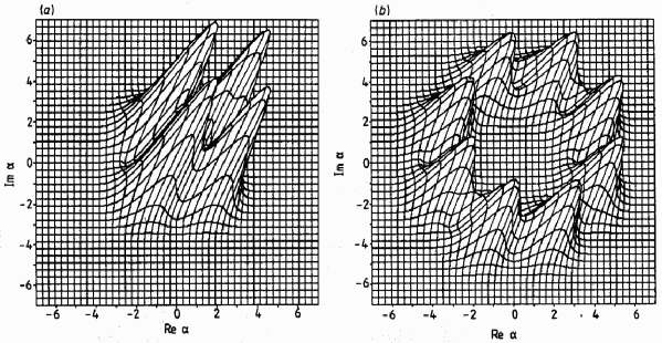
Figure 1: Plots of the quasiprobability distributed $Q(\alpha,\alpha^{*},t)$; (a) for $\alpha_{0}=2.0$ and $\tau=T_{N}/4$ (the four-peak structure) and (b) for $\alpha_{0}=4.0$ and $\tau=T_{N}/8$ (the eight-peak structure).

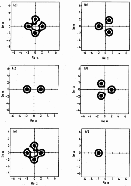
Figure 2: Contours of the quasiprobability distribution for the ‘squared’ version of the anharmonic oscillator obtained for sections at $\frac{1}{4},\frac{1}{2}$ and $\frac{3}{4}$ of the height. The parameters are $\alpha_{0}=2.0$, and (a) $\tau$ equal to $T_{S}/8$, (b) $T_{S}/6$, (c) $T_{S}/4$, (d) $T_{S}/3$, (e) $3T_{S}/8$ and (f) $T_{S}/2$.

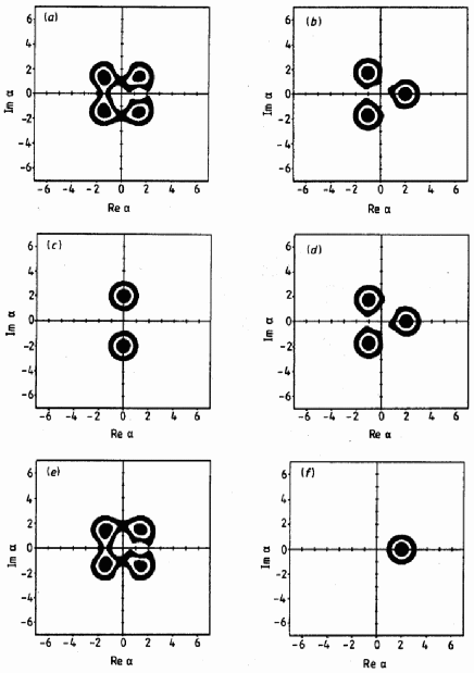
Figure 3: The same as in figure 2 but for the normally ordered version of the anharmonic oscillator. To visualise the differences between the two versions of the model, the same moments,$\tau$, are taken, that is (a) $\tau=T_{S}/8$, (b) $T_{S}/6$, (c) $T_{S}/4$, (d) $T_{S}/3$, (e) $3T_{S}/8$ and (f) $T_{S}/2$.

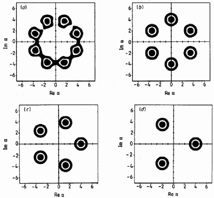
Figure 4: The same sections of the QPD for the normally ordered version of the anharmonic oscillator as in figure 3, but for the parameters: $\alpha_{0}=4.0$ and (a) $\tau$ equal to $T_{N}/8$, (b) $T_{N}/6$, (c) $T_{N}/5$, and (d) $T_{N}/3$.

In deriving equations (2an)–(2as) the superposition state (2s) has been used. It is clear from (2aq) that due to oscillations of the cosine function the interference terms can have a number of peaks. However, due to the exponential factor the amplitudes of these peaks are very small whenever the states $k$ and $l$ are well separated. ‘Well separated’ means here that $|\alpha_{k}-\alpha_{l}|^{2}\gg 1$. This gives us another criterion for good separation of states. In the following we illustrate the formation of the superposition states by showing pictures of their QPD for special situations.

Before doing this, however, we have to make some comments on the behaviour of the normally ordered version of the anharmonic oscillator. Our analytical formulae (2ag)–(2al) are for the ‘squared’ version of the anharmonic oscillator; however, it is clear from (2j) that $\theta_{N}(n)=\theta_{S}(n)-\frac{1}{2}\tau n.$ If this is inserted into equation (2i), it is seen that the superposition states obtained from the normally ordered version acquire an additional phase $\varphi=-\tau/2.$ Thus, the only change that is needed to obtain the results for this version is the replacement of the $\varphi_{k}$ by the $\varphi-\frac{1}{2}\tau$ in all the formulae obtained in this section. Geometrically this means the rotation of the QPD picture by the angle $\varphi=-\tau/2$ in the complex $\alpha$-plane, without any change in its shape. This rotation may, nevertheless, change in an essential way the general view of the QPD. For example, the QPD representing the state (2ag) is a Gaussian centred at $-\alpha_{0}$, and after the rotation by $\pi$ it becomes a Gaussian centred at $+\alpha_{0}$, that is at the initial value of $\alpha_{0}$. There is no single Gaussian peak at $\mathbf{-\alpha_{0}}$ for the normally ordered version. This is a general rule, related to the fact that the period for the normally ordered version is one half of the period for the ‘squared’ version; this will be convincingly shown in the figures.

In figure 1 we show two examples of the QPD. The first example exhibits four Gaussian peaks for the case considered by Milburn of $\alpha_{0}=2.0$. The second example shows the eight Gaussian peaks in the case $\alpha_{0}=4.0$, which according to our estimate (2am) is the maximum number of well-separated Gaussians in this case. Both examples represent quite regular shapes confirming the formation of superposition states with a definite number of components. All examples presented in our pictures are obtained numerically from the expression (2o). In figure 2 contours of the sections at $\frac{1}{4},\frac{1}{2},\frac{3}{4}$ of the height of the QPD for the ‘squared’ version of the anharmonic oscillator are presented, for $\alpha_{0}=2.0$, showing that for the maximum number of well-separated states $N_{\max}=4$ [estimated according to (2am)] the contours are not very regular circles yet, as they should be for the independent Gaussians. However, the regular four-peak structure is clearly visible. As time elapses the structures with various numbers of peaks appear which represent the superposition states given by the formulae (2ag)–(2al). The smaller the number of peaks the better is the separation of the states, and the more regular is the QPD. The sequence of the pictures is obtained for $\tau=T_{S}/8,\,T_{S}/6,\,T_{S}/4,\,T_{S}/3,\,3T_{S}/8$ and $T_{S}/2$, respectively. The identification of the QPD structures with the corresponding superposition states is quite obvious. In figure 3 the same sequence of the QPD structures is shown for the normally ordered version of the anharmonic oscillator. The differences between the two versions are quite evident. It is seen that the period for the normally ordered version is really one half of the period for the ‘squared’ version. We have chosen the same sequence of $\tau$ for both versions to visualise the differences. The structures obtained for the ‘squared’ version after half the period, which is $T_{S}/2=2\pi$, become rotations of the initial structures by the angle of $\pi$, while for the normally ordered version after the same time the initial structures are recovered. In figure 4 the contours of the QPD are presented for $\alpha_{0}=4.0$ and the normally ordered version. Again the structure with the maximum number of well-separated states, which in this case is $N_{\max}=8$, shows some irregularity, but as the number of peaks decreases the structures become more and more regular. The pictures have been obtained for $\tau=T_{N}/8,\,T_{N}/6,\,T_{N}/5$ and $T_{N}/3$, respectively. We have chosen here, as examples, two structures with even number of peaks and two structures with odd number of peaks, only. Figures 2-4 are on the same scale, which shows that the radius of the circle around which peaks are located is in figure 4 twice as large as that in figures 2 and 3, whereas the radii of the individual Gaussian bells are the same. One should also remember that the coefficients of a superposition with $N$ peaks scale as $|c_{k}|=1/\sqrt{N}$. This means that the heights of the peaks are N times lower from the single coherent-state Gaussian. If the initial number of photons $|\alpha_{0}|^{2}$ becomes large, $|\alpha_{0}|$ is large, and the maximum number of well-separated states $N_{\max}$ is also large, but the amplitudes $c_{k}$ of these states become smaller.

4 Conclusions

In this paper we have analysed the process of the generation of discrete superpositions of coherent states in the course of the evolution of the anharmonic oscillator. Two versions of an anharmonic oscillator that are used in the literature have been compared from the point of view of forming the superposition states. It has been shown that under an appropriate choice of the evolution time as a fraction of the period, the symmetry inherent in the system permits a considerable simplification of the problem of finding the coefficients of the superpositions. The number of equations that must be solved is drastically reduced by the symmetry. Some examples of the superposition states have been obtained analytically for superpositions of up to four components. General rules governing the formation of superpositions with a definite number of states have been given. The process of the formation of superposition states has been illustrated graphically by showing pictures of the corresponding quasiprobability distributions. The regular structure of the QPD that is obtained when the time (or length) becomes a fraction of the period can be easily interpreted as representing the superposition state that occurs for this time. The maximum number of well-separated states for given $|\alpha_{0}|$ has been estimated. This number becomes large when $|\alpha_{0}|$ becomes large, and regular structures of the quasiprobability distribution with a large number of Gaussian peaks can be obtained. Some of these structures have been shown in the figures. Structures with both even and odd numbers of peaks are possible. Our results shed some new light on the problem of generating discrete superpositions of coherent states and make a contribution to the discussion of the possibility of generating macroscopically-distinguishable quantum states [4, 5] as well as to the problem of the phase space interferences [16, 17].

References

- [1] Titulaer U and Glauber R J 1965 Phys. Rev. 145 1041
- [2] Stoler D 1971 Phys. Rev. D. 4 2309
- [3] Białynicka-Birula Z 1968 Phys. Rev. 173 1207
- [4] Yurke B and Stoler D 1986 Phys. Rev. Lett. 57 13
- [5] Tombesi P and Mecozzi A 1987 J. Opt. Soc. Am. B 4 1700
- [6] Tanaś R 1984 Coherence and Quantum Optics V eds L Mandel and E Wolf (New York: Plenum) p 645
- [7] Tanaś R and Kielich S 1983 Opt. Commun. 45 351; Optica Acta 31 (1984) 81
- [8] Milburn G J 1986 Phys. Rev. A 33 674
- [9] Milburn G J and Holmes C A 1986 Phys. Rev. Lett. 56 2237
- [10] Kitagawa and Yamamoto Y 1986 Phys. Rev. A 34 3974
- [11] Peřinová V and Lukš A 1988 J. Mod. Optics 35 1513
- [12] Kennedy T A B and Drummond P 1988 Phys. Rev. A 38 1319
- [13] Sanders B C 1989 Phys. Rev. A 39 4284
- [14] Vourdas A and Bishop R F 1989 Phys. Rev. A 39 214
- [15] Tanaś R 1989 Phys. Lett. 141A 217
- [16] Schleich W and Wheeler J A 1987 J. Opt. Soc. Am. B 4 1715
- [17] Schleich W, Walls D F and Wheeler J A 1988 Phys. Rev. A 38 1177