Accelerating BTZ spacetime

Abstract

An exact solution of $(2+1)$-dimensional Einstein gravity with cosmological constant is studied. The corresponding spacetime is interpreted as an accelerating BTZ spacetime. The proper acceleration, horizon structure, temperature and entropy are presented in detail. The metric being studied is very similar to the one studied by Astorino in arXiv:1101.2616, but the range of parameters is different which results in significant changes in the causal structures.

Keywords: BTZ spacetime, proper acceleration, causal structure

PACS: 04.20.Gz, 04.20.Jb

1 Introduction

In $n$-dimensional Einstein gravity, the static, spherically symmetric, vacuum black hole solution takes the form

$$\mathrm{d}s^{2}=-\left(1-\frac{m}{r^{n-3}}-\epsilon\,\frac{r^{2}}{\ell^{2}}\right)\mathrm{d}t^{2}+\left(1-\frac{m}{r^{n-3}}-\epsilon\,\frac{r^{2}}{\ell^{2}}\right)^{-1}\mathrm{d}r^{2}+r^{2}\mathrm{d}\Omega_{n-2}^{2},$$ (1)

where $m$ is a mass parameter (not necessarily equal to the mass), $\epsilon$ is the sign of the cosmological constant

$$\Lambda=\frac{(n-1)(n-2)\epsilon}{2\ell^{2}}$$

and $\mathrm{d}\Omega_{n-2}$ is the line element of an $(n-2)$-sphere. It is known that generalizations of the above metric to include the cases with non-spherical, but maximally symmetric sections exist [1, 2], i.e. the so-called topological black holes with metrics

$$\mathrm{d}s^{2}=-\left(k-\frac{m}{r^{n-3}}-\epsilon\frac{r^{2}}{\ell^{2}}\right)\mathrm{d}t^{2}+\left(k-\frac{m}{r^{n-3}}-\epsilon\frac{r^{2}}{\ell^{2}}\right)^{-1}\mathrm{d}r^{2}+r^{2}\mathrm{d}\Sigma_{n-2,k}^{2},$$ (2)

where $k=0,\pm 1$, $\mathrm{d}\Sigma_{n-2,k}^{2}$ is the line element of an $(n-2)$-dimensional maximally symmetric manifold which can be written explicitly as

$$\mathrm{d}\Sigma_{n-2,k}^{2} =\mathrm{d}\theta_{1}^{2}+\rho_{k}^{2}(\theta_{1})\mathrm{d}\Omega_{n-3}^{2},\qquad\rho_{k}(\theta_{1})=\left\{\begin{array}[]{ll}\sin\theta_{1}&(k=+1)\cr\theta_{1}&(k=0)\cr\sinh\theta_{1}&(k=-1)\end{array}\right.$$ (6)

where $\mathrm{d}\Omega_{n-3}^{2}$ is the line element of an $(n-3)$-sphere. The choices $k=0,-1$ are allowed only for $\epsilon=-1$, i.e. the asymptotically AdS case. For all dimensions $n>3$, the metrics (2) are distinct for different values of $k$. However, for $n=3$, i.e. the case of BTZ black holes, there is some ambiguity, because there is no difference between $\mathrm{d}\Omega_{1}^{2}$ and $\mathrm{d}\Sigma_{1,k}^{2}$ and one can absorb $k$ into the mass parameter $m$ (as is usually done in the literature, see [3] for instance).

The study of Einstein gravity in three spacetime dimensions with cosmological constant was initiated in [4]. In the absence of matter source, this theory is locally trivial because of the lack of propagating degrees of freedom. In spite of this fact, there can be nontrivial boundary degrees of freedom and these are very interesting thanks to the AdS/CFT duality: the CFT dual of 3D gravity is $(1+1)$-dimensional, with infinite conformal symmetries making it completely integrable [5]. In the light that higher dimensional CFTs are often mathematically difficult to treat, one often take three dimensional gravity as an ideal toy model for learning essential properties of the AdS/CFT duality. In this regard, various generalizations of BTZ black hole spacetime and their holographic properties have been studied extensively (see [6, 7, 8, 9, 10, 11, 12] for a very incomplete list of related works).

In a recent paper [13], Astorino studied an accelerating variant of the BTZ black hole. Basically, the spacetime metric obtained in [13] is a conformally transformed version of the 3D version of the metric (1), though the notations used are slightly different. This accelerating BTZ spacetime enjoys some feature which are otherwise absent in the non-accelerating version, e.g. the presence of black holes with an angular singularity, allowing extensions to black string of finite length and black ring in 4-dimensions, etc. Some properties of the spacetime are analyzed in detail in [13], including horizon structure, temperature and entropy of the black holes in certain range of the parameters. In this paper, we shall extend the work of [13] and analyze the accelerating BTZ spacetime, allowing the acceleration parameter to take a different sign from that in [13]. We also prefer to rewrite the metric of in a form which is conformal to the 3D version of (2), taking advantage of the ambiguity in choosing parameters in the 3D case mentioned above.

2 Metric and proper acceleration

We begin by writing the spacetime metric in the following form,

$$\mathrm{d}s^{2}=\frac{1}{\gamma(r,\theta)^{2}}\left[-f(r)\mathrm{d}t^{2}+f(r)^{-1}\mathrm{d}r^{2}+r^{2}\mathrm{d}\theta^{2}\right],$$ (7)

where

$$\gamma(r,\theta)=\alpha\,r\cosh(\sqrt{m-k}\,\theta)-1,$$ (8)

$$f(r)=k-m-\epsilon\,\frac{r^{2}}{\ell^{2}},$$ (9)

where $k=0,\pm 1$, $\epsilon=0,\pm 1$ and $\ell$ is a positive parameter. Clearly, this is an exact solution to the 3D vacuum Einstein with cosmological constant $\Lambda$, which is given in terms of the parameters as

$$\Lambda=\alpha^{2}(m-k)+\frac{\epsilon}{\ell^{2}}.$$ (10)

For comparison, we also rewrite the original metric presented in [13] as follows:

$$\mathrm{d}s^{2} =\frac{1}{\left(1+\alpha\,r\,\cos\left(\sqrt{1-m}\,\theta\right)\right)^{2}}\bigg{\{}-\left[1-m+r^{2}\left[\alpha^{2}(m-1)-\Lambda\right]\right]\mathrm{d}t^{2}$$

$$\qquad+\left[1-m+r^{2}\left[\alpha^{2}(m-1)-\Lambda\right]\right]^{-1}\mathrm{d}r^{2}+r^{2}\mathrm{d}\theta^{2}\bigg{\}}.$$

There are several differences in our presentation (7) of the metric from the one given in [13]. First, we allow $k$ to take 3 possible values $0,\pm 1$ rather than fix it to the value 1. The reason for this is to stress that for all 3 choices of values of $k$, the $m=0$ limit of the metric are just Einstein vacua, rather than black hole spacetimes [14, 15] (for $k=\pm 1$, the corresponding vacua are accelerating vacua, see below. Among these, the $k=1,m=0,\epsilon=1$ vacuum was first found and analyzed in [16].). Besides this purpose, there is no need to distinguish between $k$ and $m$ and the combination $m-k$ can be viewed as a single parameter. Second, we made a change $\cos(\sqrt{k-m}\,\theta)\rightarrow\cosh(\sqrt{m-k}\,\theta)$. Though this is an identity transform, the use of hyperbolic cosine reflects the actual angular behavior of the conformal factor in the presence of black hole which needs $m>k$, see below. The third and perhaps the most significant difference lies in that the parameter $\alpha$ in our notation is actually $-\alpha$ in [13]. In the analysis of [13], an implicit assumption of $\alpha>0$ was used (i.e. $\alpha<0$ in our notation), so we shall be dealing only with the choice $\alpha>0$.

The coordinate ranges for $t$ and $r$ are specified as follows: $-\infty<t<\infty$, $0\leq r<\infty$. As for the coordinate $\theta$, due to the lack of translational symmetry in $\theta$ in the presence of the conformal factor, we seem to have no reason to restrict it to be in $[-\pi,\pi]$. However, we still wish to interpret the coordinates $(r,\theta)$ as being polar, just as in the standard case of BTZ black hole [3], since the latter is the $\alpha=0$ limit of our solution (7). Thus we make the choice $-\pi\leq\theta\leq\pi$. We shall see later that in some cases the range for $\theta$ still need to be adjusted for observers living in one side of the conformal infinity. The necessity of adjusting the range of $\theta$ in certain cases is one of the major point we would like to make with our choice of $\alpha$, in contrast to the cases analyzed in [13].

Let us recall the explanation of the conformal factor $1/\gamma^{2}$ in the metric (7). Consider a static observer

$$x^{\mu}(\lambda)=\left(\lambda\frac{\alpha\,r\cosh(\sqrt{m-k}\,\theta)-1}{\sqrt{k-m-\epsilon\,\frac{r^{2}}{\ell^{2}}}},r,\theta\right)$$

in the spacetime, where $\lambda$ is the proper time. It is easy to see that the proper acceleration $a^{\mu}=u^{\nu}\nabla_{\nu}u^{\mu}$ (where $u^{\mu}=\frac{\mathrm{d}x^{\mu}}{\mathrm{d}\lambda}$) has a norm equal to

$$a^{\mu}a_{\mu}=-\Lambda+\left(\frac{\epsilon}{\ell^{2}}\right)\frac{(k-m)(\alpha\,r\cosh\left(\sqrt{m-k}\,\theta\right)-1)^{2}}{k-m-\epsilon\,\frac{r^{2}}{\ell^{2}}}.$$

At $r=0$, this reduces to

$$a^{\mu}a_{\mu}=\alpha^{2}(k-m).$$ (11)

This shows that $\alpha$ is proportional (but not equal) to the magnitude $|a|$ of the proper acceleration at the origin if $m\neq k$. Thus $\alpha$ may be called an acceleration parameter. Let us remark that the $t$-component of $a^{\mu}$ is zero. Because of this, $a^{\mu}$ is spacelike and we ought to have $a^{\mu}a_{\mu}>0$ in the static region of the spacetime. Combining with (11), we see that $r=0$ is not in the static region if $m>k$. That the region of spacetime containing the origin $r=0$ is non-static is typical for black holes centered at the origin. For this reason, we infer that an accelerating black hole can exist only for $m>k$.

3 Horizon, temperature and entropy

Now let us study the horizon structure. In general, zeros of $f(r)$ correspond to horizons. In our case the zeros are located at

$$r_{H}=\ell\sqrt{\frac{k-m}{\epsilon}}.$$

This excludes, in particular, the possibility of choosing $\epsilon=0$. For a real zero to exist, we need either (i) $\epsilon=+1$ with $m<k$, or (ii) $\epsilon=-1$ with $m>k$.

Notice that, according to (10), the sign of $\epsilon$ alone cannot determine whether the solution is asymptotically de Sitter or anti-de Sitter. We can re-express the cosmological constant in terms of $r_{H}$ as

$$\Lambda =\frac{\epsilon}{\ell^{2}}(1-\alpha^{2}r_{H}^{2}).$$

Therefore, for $\epsilon=+1$, we need $\alpha\,r_{H}>1$ to make an AdS background, $\alpha\,r_{H}<1$ to make a dS background, whereas for $\epsilon=-1$, $\alpha\,r_{H}>1$ makes a dS background and $\alpha\,r_{H}<1$ makes an AdS background. For either choices of $\epsilon$, $\alpha\,r_{H}=1$ corresponds to a flat background.

The choice (i) (i.e $\epsilon=+1$, $m<k$) corresponds to the case in which static observers are located inside the horizon (i.e. $r<r_{H}$), hence the horizon is more like a cosmological horizon rather than a black hole horizon. Note that, in this case, the hyperbolic cosine function $\cosh(\sqrt{m-k}\,\theta)$ in the conformal factor is actually the usual trigonometric cosine $\cos(\sqrt{k-m}\,\theta)$. Since $a^{\mu}a_{\mu}>0$ at $r=0$, the static region in this spacetime is surrounded by an accelerating horizon at $r=r_{H}$ which is not a black hole.

The choice (ii) ($\epsilon=-1$, $m>k$) corresponds to the case in which static observers are located outside the horizon (i.e. $r>r_{H}$), which is the case for a black hole solution. so we shall be concentrating only on this choice and bear in mind

$$r_{H}=\ell\sqrt{m-k},\qquad\Lambda=\frac{1}{\ell^{2}}(\alpha^{2}r_{H}^{2}-1)$$

from now on.

Notice that for the black hole case with $\epsilon=-1,m>k$, the cosmological constant $\Lambda$ needs not to be negative. This seems to be in contradiction with the known no-go theorem proposed by Ida [17], which roughly says that the existence of a black hole horizon in $(2+1)$ dimensions requires a negative cosmological constant. The reason that our solution evades this no-go theorem is because that the proof of the theorem depends on the assumption that the curve corresponding to the horizon is everywhere smooth, however in our case the horizon contains an angular singularity along $\theta=\pm\pi$, which represents a string or strut acting on the horizon as the source of the acceleration. Similar situations have also been encountered in [13]. We will come back to this point later.

There are a number of standard ways to calculate the temperature at the horizon. For instance, we may take the timelike Killing vector $\chi=\partial_{t}$ to get the surface gravity $\kappa=\sqrt{-\frac{1}{2}\nabla^{\mu}\chi^{\nu}\nabla_{\mu}\chi_{\nu}}$ and then using $T=\frac{\kappa}{2\pi}$ to evaluate the temperature. The result reads

$$\kappa=\frac{\sqrt{m-k}}{\ell},\qquad T=\frac{\sqrt{m-k}}{2\pi\ell}.$$

Another simple shortcut to the evaluation of the horizon temperature is to make use of the formula

$$T=\frac{1}{4\pi}\left.\sqrt{\frac{\mathrm{d}g_{00}}{\mathrm{d}r}\frac{\mathrm{d}(g_{11}^{-1})}{\mathrm{d}r}}\right|_{r=r_{H}},$$

which is valid for any diagonal metric.

Now let us look at the function $\gamma(r,\theta)$ (eq.(8)) appearing in the conformal factor. Every zero of $\gamma(r,\theta)$ represents a conformal infinity in the metric (7). If the the acceleration parameter $\alpha$ were negative, then $\gamma(r,\theta)$ will never have a zero for $r>0$, provided $m>k$. So one does not need to worry about the conformal infinities. This is the case for [13]. In our case, however, conformal infinity does exist because we are interested in the choice $\alpha>0$. Moreover, the conformal infinity can intersect with the horizon if $0<\alpha r_{H}\leq 1$, i.e. in the AdS or flat cases. This can be seen from the fact that the equation $\gamma(r_{H},\theta)=0$ has two solutions $\theta=\pm\theta_{0}$, with

$$\theta_{0}=\frac{1}{\sqrt{m-k}}\,\mathrm{arccosh}\left(\frac{1}{\alpha\,r_{H}}\right).$$ (12)

If $\theta_{0}\in[0,\pi]$, then the intersection appears. From the outside static observer’s point of view, this means that the horizon stretches all the way through infinity, i.e. it is noncompact. While evaluating the area of such horizons, one should exclude the part of the $r=r_{H}$ hyper surface that is hidden beyond the conformal infinity.

Recall that the conformal infinity separates the spacetime into two patches: the $(-)$ patch $\gamma(r,\theta)\leq 0$ and the $(+)$ patch $\gamma(r,\theta)\geq 0$. Each observer can perceive only one of the two patches. Therefore, the determination for the correct range for $\theta$ in the $\alpha\,r_{H}\leq 1$ cases depends on which patch the observer lives in. For the AdS case with $\theta_{0}\in[0,\pi]$, we need to choose $\theta\in[-\theta_{0},\theta_{0}]$ in the $(-)$ patch and $\theta\in[-\pi,-\theta_{0})\cup(\theta_{0},\pi]$ in the $(+)$ patch. For the AdS case with $\theta_{0}>\pi$, the horizon will lie completely in the $(-)$ patch and we can still choose $\theta\in[-\pi,\pi]$. The flat case corresponds to $\theta_{0}=0$, the horizon intersects with the conformal infinity at a single point $\theta=0$ in the $(+)$ patch, in which case we need to choose $\theta\in[-\pi,0)\cup(0,\pi]$, and there is no horizon in the $(-)$ patch. For the de Sitter case, the zeros of $\gamma(r,\theta)$ does not intersect with the horizon and we still choose $\theta\in[-\pi,\pi]$. The presence of the conformal infinity makes the analysis of the entropy and angular singularities of the horizon significantly different from the case of [13], as is shown below.

First let us consider the entropy of the black hole spacetimes. We assume that the Beckenstein-Hawking relation for the entropy still holds. For the asymptotically dS case (i.e. $\alpha\,r_{H}>1$). The horizon lies entirely in the $(+)$ patch, and the entropy is

$$S=\frac{1}{4}\int^{\pi}_{-\pi}\left.\sqrt{g_{\theta\theta}}\right|_{r=r_{H}}\mathrm{d}\theta=\frac{\ell}{\sqrt{\alpha^{2}r_{H}^{2}-1}}\mathrm{arctan}\left[\frac{\alpha r_{H}+1}{\sqrt{\alpha^{2}r_{H}^{2}-1}}\tanh\left(\frac{\pi}{2}\sqrt{m-k}\right)\right].$$

For the asymptotically flat case, the horizon hits the conformal infinity at a single point $\theta=0$ in the $(+)$ patch, whereas there is no horizon in the $(-)$ patch. Therefore, we only need to evaluate the entropy in the $(+)$ patch, yielding a divergent result. The asymptotically AdS case must be subdivided into two subcases, i.e. $\theta_{0}\in[0,\pi]$ and $\theta_{0}>\pi$. For $\theta_{0}\in[0,\pi]$, we have

$$\displaystyle S =\frac{1}{4}\int^{\theta_{0}}_{-\theta_{0}}\left.\sqrt{g_{\theta\theta}}\right|_{r=r_{H}}\mathrm{d}\theta$$

$$=\frac{\ell}{\sqrt{1-\alpha^{2}r_{H}^{2}}}\mathrm{arctanh}\left[\frac{1+\alpha r_{H}}{\sqrt{1-\alpha^{2}r_{H}^{2}}}\tanh\left(\frac{1}{2}\mathrm{arccosh}\left(\frac{1}{\alpha r_{H}}\right)\right)\right]$$

in the $(-)$ patch and

$$S =\frac{1}{4}\left(\int^{-\theta_{0}}_{-\pi}+\int^{\pi}_{\theta_{0}}\right)\left.\sqrt{g_{\theta\theta}}\right|_{r=r_{H}}\mathrm{d}\theta$$

$$=\frac{\ell}{\sqrt{1-\alpha^{2}r_{H}^{2}}}\left\{\mathrm{arctanh}\left[\frac{1+\alpha r_{H}}{\sqrt{1-\alpha^{2}r_{H}^{2}}}\tanh\left(\frac{\pi}{2}\sqrt{m-k}\right)\right]\right.$$

$$\qquad\left.-\mathrm{arctanh}\left[\frac{1+\alpha r_{H}}{\sqrt{1-\alpha^{2}r_{H}^{2}}}\tanh\left(\frac{1}{2}\mathrm{arccosh}\left(\frac{1}{\alpha r_{H}}\right)\right)\right]\right\}$$

in the $(+)$ patch. For $\theta_{0}>\pi$, we have

$$S=\frac{1}{4}\int^{\pi}_{-\pi}\left.\sqrt{g_{\theta\theta}}\right|_{r=r_{H}}\mathrm{d}\theta=\frac{\ell}{\sqrt{1-\alpha^{2}r_{H}^{2}}}\mathrm{arctanh}\left[\frac{1+\alpha r_{H}}{\sqrt{1-\alpha^{2}r_{H}^{2}}}\tanh\left(\frac{\pi}{2}\sqrt{m-k}\right)\right]$$

in the $(-)$ patch and there is no horizon in the $(+)$ patch.

Next comes the analysis on the angular singularities of the horizon. Such singularities exists in all cases mentioned above because of the jump in the derivatives of $\gamma(r,\theta)$ at $\theta=\pm\pi$, and they provides the source of the acceleration which may be interpreted as a string or strut tied up to the horizon along the $\theta=\pm\pi$ direction. The tension $\tau$ of the string or strut may be calculated using the jump of the exterior curvature at the singularity using the formula [13]

$$[\mathcal{K}_{\mu\nu}]_{\theta=-\pi}^{\theta=\pi}-h_{\mu\nu}[\mathcal{K}]_{\theta=-\pi}^{\theta=\pi}=-h_{\mu\nu}\tau$$ (13)

where $h_{\mu\nu}=g_{\mu\nu}-n_{\mu}n_{\nu}$ is the induced metric on the $\theta=\pm\pi$ surface, $\mathcal{K}=\mathcal{K}_{\mu\nu}h^{\mu\nu}$, and $\mathcal{K}_{\mu\nu}=\frac{1}{2}\mathcal{L}_{n}h_{\mu\nu}$ is the exterior curvature (with $\mathcal{L}_{n}$ representing the Lie derivative with respect to the normal vector $n^{\mu}$). Applying (13) to the present case, we find that $\tau$ is negative in all cases except in the asymptotically AdS case with $\theta_{0}>\pi$. Actually, the horizon surface stretches to the direction $\theta=\pm\pi$ in the $(+)$ patch in all cases except the exceptional case mentioned above in which it goes to the $(-)$ patch. The explicit value of $\tau$ is

$$\tau=-2\alpha\sqrt{m-k}\sinh(\pi\sqrt{m-k})$$ (14)

if the horizon reaches $\theta=\pm\pi$ in the $(+)$ patch, or

$$\tau=2\alpha\sqrt{m-k}\sinh(\pi\sqrt{m-k})$$ (15)

if the horizon reaches $\theta=\pm\pi$ in the $(-)$ patch. The tension depends on the difference $m-k$ and it vanishes at $m=k$ or $m=0,k=1$. Besides the vanishing points, $\tau>0$ corresponds to a pushing strut and $\tau<0$ corresponds to a pulling string.

Let us stress that, while doing the above analysis, we have not considered the possibility of extending the spacetime to the $r<0$ regime. If the latter regime were also included, then we will have an extra horizon with $r_{H}<0$ as well as an extra conformal infinity at $r<0$ (if $\alpha$ were chosen negative). In any case the positive conformal infinity at $r>0$ and the negative conformal infinity at $r<0$ cannot be both present for a fixed $\alpha$. Note that this last statement applies only to the black hole case ($m>k$). If we were considering the bubble spacetime with $m<k$, then the two conformal infinities will be both present for any given $\alpha$.

The mass or energy of the black hole solution is difficult to determine, because there is no known way to determine the mass of asymptotically non-flat, accelerating black holes. Nevertheless, since at $m=0$, the metric (7) becomes the accelerating vacua described recently by us [15], we see that the mass of the black hole has to be proportional to $m$ by dimensional analysis. One may, of course, assume that the first law of black hole thermodynamics holds in this situation and use that to calculate the mass of the black hole, as did in [13]. However, we prefer not to proceed in that direction due to the following reasons. One the one hand, the usual logic on the black hole thermodynamics is that the correctness of the first law of black hole physics ought to be checked after each observable of the black hole spacetime has been evaluated by other means, if gravity and black hole thermodynamic were considered as independent of each other. On the other hand, for spacetimes with non-vanishing cosmological constant (which is the case of our main interests), the presentation of the first law contains some ambiguity even one is sure about its correctness. One may, for instance, consider the cosmological constant as being the pressure of some liquid component and then write the first law in a form like $dE=TdS-pdV$ (see, e.g. [18]), rather than simply $dE=TdS$. In view of this, the first law alone is still insufficient to determine the mass of the black hole, even if we accept the correctness of the first law by ad hoc assumption.

4 Extrinsic geometric description of the solution

Unlike black hole solutions in dimensions $n>3$, the 3D black holes enjoys a very particular property, i.e. the Riemann curvature can be written as

$$R_{\mu\nu\rho\sigma}=\Lambda(g_{\mu\rho}g_{\nu\sigma}-g_{\mu\sigma}g_{\nu\rho}).$$

This allows us to embed some coordinate patch of the black hole spacetime into appropriate 4D flat spacetime and study it from an extrinsic geometric point of view.

As in the previous section, we shall be working only with the choice (ii), i.e. $\epsilon=-1$, $m>k$, with the presence of black hole horizon in our solution. We shall present the embedding relations according to different asymptotics of the solution.

First we consider the asymptotically de Sitter case ($\alpha r_{H}>1$). In this case, the spacetime can be embedded in a 4D Minkowski spacetime

$$\mathrm{d}s^{2}=-(\mathrm{d}X_{0})^{2}+(\mathrm{d}X_{1})^{2}+(\mathrm{d}X_{2})^{2}+(\mathrm{d}X_{3})^{2}$$

as a hyperboloid,

$$-(X_{0})^{2}+(X_{1})^{2}+(X_{2})^{2}+(X_{3})^{2}=\frac{\ell^{2}}{\lambda^{2}},$$

where

$$\lambda=\sqrt{\alpha^{2}\,r_{H}^{2}-1}=\sqrt{\alpha^{2}(m-k)\ell^{2}-1}.$$ (16)

The coordinate transformation leading to our solution (7) is given as

$$X_{0} =\frac{1}{\gamma\sqrt{m-k}}\sqrt{r^{2}-(m-k)\,\ell^{2}}\,\sinh\frac{\sqrt{m-k}\,t}{\ell},$$ (17)

$$X_{1} =\frac{1}{\gamma\sqrt{m-k}}\sqrt{r^{2}-(m-k)\,\ell^{2}}\,\cosh\frac{\sqrt{m-k}\,t}{\ell},$$ (18)

$$X_{2} =\frac{1}{\gamma\sqrt{m-k}}\,r\sinh\left(\sqrt{m-k}\,\theta\right),$$ (19)

$$X_{3} =\frac{1}{\gamma\sqrt{m-k}}\,\lambda^{-1}\left(-r\cosh(\sqrt{m-k}\,\theta)+\alpha\sqrt{m-k}\,\ell^{2}\right),$$ (20)

where $\gamma=\gamma(r,\theta)$ is given in (8). Notice that at $m=k$, the embedding breaks down, although the original metric (7) is well defined in that case, which corresponds to an accelerating AdS vacuum. Meanwhile, the embedding equations hold only for $r\geq r_{H}$, i.e. the static region of outside the horizon and the horizon itself, thus do not cover the whole spacetime.

The case of AdS black hole spacetime ($\alpha\,r_{H}<1$) can be embedded in a 4D pseudo Minkowski spacetime

$$\mathrm{d}s^{2}=-(\mathrm{d}X_{0})^{2}+(\mathrm{d}X_{1})^{2}+(\mathrm{d}X_{2})^{2}-(\mathrm{d}X_{3})^{2}$$

as a hyperboloid,

$$-(X_{0})^{2}+(X_{1})^{2}+(X_{2})^{2}-(X_{3})^{2}=-\frac{\ell^{2}}{\lambda^{2}}.$$

The embedding relations are the same as (17)-(20), but with $\lambda$ replaced by

$$\lambda=\sqrt{1-\alpha^{2}\,r_{H}^{2}}=\sqrt{1-\alpha^{2}(m-k)\ell^{2}}.$$ (21)

The flat case, $\alpha\,r_{H}=1$, is even more simpler: it can be seen that the asymptotically flat black hole metric

$$\mathrm{d}s^{2}=\frac{1}{\gamma^{2}}\left[-(m-k)(-1+\alpha^{2}r^{2})\mathrm{d}t^{2}+\frac{\mathrm{d}r^{2}}{(m-k)(-1+\alpha^{2}r^{2})}+r^{2}\mathrm{d}\theta^{2}\right]$$

can be obtained from the 3D Minkowski metric

$$\mathrm{d}s^{2}=-\mathrm{d}X_{0}^{2}+\mathrm{d}X_{1}^{2}+\mathrm{d}X_{2}^{2},$$

thanks to the coordinate transformation

$$X_{0} =\frac{1}{\gamma\alpha\sqrt{m-k}}\sqrt{\alpha^{2}r^{2}-1}\sinh(\alpha(m-k)t),$$

$$X_{1} =\frac{1}{\gamma\alpha\sqrt{m-k}}\sqrt{\alpha^{2}r^{2}-1}\cosh(\alpha(m-k)t),$$

$$X_{2} =\frac{1}{\gamma\sqrt{m-k}}r\sinh(\sqrt{m-k}\theta).$$

Let us stress once again that this extrinsic geometric description covers only a small portion of the black hole spacetime ($\alpha r>1$). It helps us to understand the flat nature of the spacetime, but it doesn’t provides us with a global view of the spacetime.

The accelerating bubble spacetime corresponding to $\epsilon=+1$ and $m<k$ in (7) can also be embedded into appropriate 4D target spacetimes following a similar spirit.

5 Causal structure of the spacetime

The extrinsic geometric description of the metric can only describe a small coordinate patch of the spacetime which lies outside the horizon. To fully understand the structure of the spacetime, we identify its causal structure. As in the previous section, we shall be working only with the choice $\epsilon=-1,m>k$, i.e. black hole cases.

As usual, we introduce the Eddington-Finkelstein coordinates,

$$u=t-r^{*},\quad v=t+r^{*},$$ (22)

where the tortoise coordinate $r^{*}$ is defined as

$$r^{*}=\int(k-m+r^{2}/\ell^{2})^{-1}\mathrm{d}r=\frac{\ell}{2\sqrt{m-k}}\log\left|\frac{r-r_{H}}{r+r_{H}}\right|,$$ (23)

and both $u$ and $v$ belong to the range $(-\infty,\infty)$. In this coordinate the metric becomes

$$\mathrm{d}s^{2}=\rho^{2}\left[-\left(k-m+\frac{r^{2}}{\ell^{2}}\right)\mathrm{d}u\mathrm{d}v+r^{2}\mathrm{d}\theta^{2}\right],$$ (24)

where $\rho=\left(\alpha r\cosh(\sqrt{m-k}\,\theta)-1\right)^{-1}=\gamma(r,\theta)^{-1}$. The Kruskal-like coordinates are introduced as

$$\tilde{u}=\pm\exp\left(-\frac{\sqrt{m-k}}{\ell}u\right),\quad\tilde{v}=\pm\exp\left(\frac{\sqrt{m-k}}{\ell}v\right),$$

where $\tilde{u}$ and $\tilde{v}$ takes the same sign if $r<r_{H}$, and they take opposite signs if $r\geq r_{H}$. So there are totally 4 different combinations, each of which corresponds to a causal patch in the conformal diagrams to be drawn below. In each cases, one finds that

$$\tilde{u}\tilde{v}=-\frac{r-r_{H}}{r+r_{H}},$$ (25)

and eq.(24) becomes

$$\mathrm{d}s^{2}=\rho^{2}\left[-\frac{(r+r_{H})^{2}}{m-k}\mathrm{d}\tilde{u}\mathrm{d}\tilde{v}+r^{2}\mathrm{d}\theta^{2}\right],$$ (26)

where $r$ and $\rho$ are to be regarded as functions of $\tilde{u}$ and $\tilde{v}$,

$$r =r_{H}\frac{1-\tilde{u}\tilde{v}}{1+\tilde{u}\tilde{v}},$$

$$\rho =\frac{1+\tilde{u}\tilde{v}}{\alpha r_{H}(1-\tilde{u}\tilde{v})\cosh(\sqrt{m-k}\theta)-(1+\tilde{u}\tilde{v})}.$$

Finally, the Carter-Penrose coordinates can be introduced by the usual arctangent mappings of $\tilde{u}$ and $\tilde{v}$

$$U =\arctan{\tilde{u}},\quad V=\arctan{\tilde{v}},$$

$$T \equiv U+V,\quad R\equiv U-V,$$

in terms of which the metric becomes

$$\mathrm{d}s^{2}=\frac{\rho^{2}\ell^{2}}{\cos{R}^{2}}\left[-\mathrm{d}T^{2}+\mathrm{d}R^{2}+\frac{r^{2}}{\ell^{2}}\cos^{2}(R)~{}\mathrm{d}\theta^{2}\right].$$ (27)

The values of the product $\tilde{u}\tilde{v}$ at $r=r_{H}$, $\rho=0$, $r=0$ and $\rho=\infty$ are respectively

$$\lim_{r\rightarrow r_{H}}\tilde{u}\tilde{v} =0,\quad\Rightarrow UV=0$$

$$\lim_{\rho\rightarrow 0}\tilde{u}\tilde{v} =-1,\quad\Rightarrow U-V=\pm\frac{\pi}{2}$$

$$\lim_{r\rightarrow 0}\tilde{u}\tilde{v} =1,\quad\Rightarrow U+V=\pm\frac{\pi}{2}$$

$$\lim_{\rho\rightarrow\infty}\ \tilde{u}\tilde{v} =\frac{\alpha r_{H}\cosh(\sqrt{m-k}\theta)-1}{\alpha r_{H}\cosh(\sqrt{m-k}\theta)+1}.$$

These correspond to the various boundaries in the Carter-Penrose diagrams. Among these, the first three sets of boundaries corresponding to $r=r_{H}$, $\rho=0$ and $r=0$ can easily be depicted, and in fact they constitute the Penrose diagram for the static, non-rotating and non-accelerating BTZ black hole [19]. However, the forth set of the boundary, i.e. that corresponding to the conformal infinity $\rho=\infty$, depends on both the multiplication $\alpha r_{H}$ (i.e. on the cosmological constant) and the angular variable $\theta$. So we need to consider the causal diagrams separately for different choices of cosmological constant and the angle $\theta$.

5.1 $\Lambda>0$

Since for $\Lambda>0$ we have $\alpha r_{H}\cosh(\sqrt{m-k}\theta)>1$, so $0<\lim_{\rho\rightarrow\infty}\tilde{u}\tilde{v}<1$. The Carter-Penrose diagram in this case consists of the coordinate poles represented by the lines $\rho=0$, $r=0$, the horizon at $r=r_{H}$ and the (curved) past and future conformal infinities at $\rho=\infty$. The corresponding diagram is depicted as in Fig.1.

In this and all subsequent figures, lines labeled with $r=r_{H}$ represent acceleration horizons, $I^{+}$ and $I^{-}$ are respectively past and future infinities ($\rho=+\infty$ or $r=\frac{1}{\alpha\cosh(\sqrt{m-k}\theta)}$), and $\rho=0$ or $I$ correspond to $r=+\infty$, the spacelike infinities.

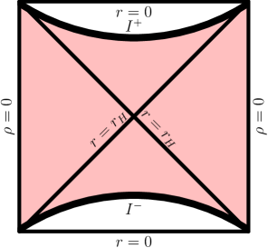
Figure 1: Carter-Penrose diagrams for $\Lambda>0$: shaded area corresponds to the ($+$) patch, unshaded areas correspond to the ($-$) parch.

5.2 $\Lambda=0$

In this case, we have $r_{H}=\frac{1}{\alpha}\geq\frac{1}{\alpha\cosh(\sqrt{m-k}\theta)}$, where equality holds only for $\theta=\theta_{0}=0$. The procedure for drawing Carter-Penrose diagrams for the case $\Lambda=0$ is very similar to the case $\Lambda>0$, except that we need to consider two subcases:

• $\theta\neq 0$ (i.e. $\theta\in[-\pi,0)\cup(0,\pi]$): we have $0<\lim_{\rho\rightarrow\infty}\ \tilde{u}\tilde{v}<1$. The Carter-Penrose diagram is depicted in Fig.2 (a);

• $\theta=0$: in this case $\lim_{\rho\rightarrow\infty}\ \tilde{u}\tilde{v}=0.$ The Carter-Penrose diagram is depicted in Fig.2 (b).

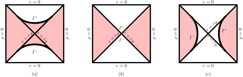
Figure 2: Carter-Penrose diagrams for $\Lambda\leq 0$.

5.3 $\Lambda<0$

In this case, we have $r_{H}<\frac{1}{\alpha}$. The procedure to get the conformal diagrams is more involved because we need to consider two subcases $\theta_{0}\in[0,\pi]$ and $\theta_{0}>\pi$.

5.3.1 $\theta_{0}\in[0,\pi]$

In this case,

$$\lim_{\rho\rightarrow\infty}\ \tilde{u}\tilde{v} =\frac{\alpha r_{H}\cosh(\sqrt{m-k}\theta)-1}{\alpha r_{H}\cosh(\sqrt{m-k}\theta)+1}$$

$$=\frac{\cosh(\sqrt{m-k}\theta)-\cosh(\sqrt{m-k}\theta_{0})}{\cosh(\sqrt{m-k}\theta)+\cosh(\sqrt{m-k}\theta_{0})}.$$

We need to subdivide the range of $\theta$ into three subcases: $\theta\in[-\pi,-\theta_{0})\cup(\theta_{0},\pi]$, $\theta=\pm\theta_{0}$ and $\theta\in(-\theta_{0},\theta_{0})$.

• $\theta\in[-\pi,-\theta_{0})\cup(\theta_{0},\pi]$: we have again $0<\lim_{\rho\rightarrow\infty}\ \tilde{u}\tilde{v}<1$ and the Carter-Penrose diagram is similar to the $\Lambda>0$ case and is depicted in Fig.2 (a).

• $\theta=\pm\theta_{0}$: in this case $\lim_{\rho\rightarrow\infty}\ \tilde{u}\tilde{v}=0$. The Carter-Penrose diagram is shown in Fig.2 (b).

• $\theta\in(-\theta_{0},\theta_{0})$: we have $-1<\lim_{\rho\rightarrow\infty}\ \tilde{u}\tilde{v}<0$. The Carter-Penrose diagram is depicted in Fig.2 (c).

5.3.2 $\theta_{0}>\pi$

In this case we have $-1<\lim_{\rho\rightarrow\infty}\ \tilde{u}\tilde{v}<0$. The Carter-Penrose diagram is depicted in Fig.3.

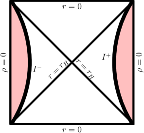
Figure 3: Carter-Penrose diagrams for $\Lambda<0$.

6 Conclusion

In this paper, we have made a detailed analysis of the accelerating BTZ spacetime (7). The proper acceleration, horizon structure, temperature and entropy are presented in detail. The presence of the accelerating parameter $\alpha$ has resulted in some new features comparing to the case of static BTZ spacetime. For instance, black hole horizon exists only in AdS background with $m>1$ in the static case, however, in the presence of the acceleration parameter, black hole horizons exist for all possible signs of $\Lambda$, provided the parameter $\epsilon$ takes the value $-1$ and $m>k$ (we should take $m>0$ for $k=-1$ if positive mass is required). In addition, even if $\epsilon=+1$ we still have horizons which corresponds to accelerating bubbles which are structures absent in the static case.

Comparing to the case of [13], our choice of the parameter range, especially the choice of sign for $\alpha$, has resulted in significant changes in the causal structure of the spacetime. The unexpected rich structure in the causal diagrams makes the spacetime more interesting than the static BTZ black hole.

In closing, let us mention that the accelerating BTZ spacetime discussed in this article can be viewed as the 3D analogue of the C-metric in 4-dimensions. It is well known that the C-metric in 4D can be both charged and rotating [20, 21]. However, the solution we discussed in this article is only the analogue of the uncharged, non-rotating version. It will be interesting to ask whether one can find the accelerating version of charged and/or rotating BTZ spacetimes in 3 dimensions. It is also tempting to ask whether the presence of proper acceleration can give rise to some novel features in the holographic dual picture. We leave these problems to future studies.

References

- [1] R. B. Mann, “Pair Production of Topological anti de Sitter Black Holes,” Class.Quant.Grav.14: L109-L114, 1997 [arXiv: gr-qc/9607071].
- [2] D. Birmingham, “Topological Black Holes in Anti-de Sitter Space,” Class.Quant.Grav. 16 (1999) 1197-1205 [arXiv: hep-th/9808032].
- [3] M. Bañados, C. Teitelboim, and J. Zanelli, “The Black Hole in Three Dimensional Space Time,” Phys.Rev.Lett. 69 (1992) 1849-1851 [arXiv: hep-th/9204099].
- [4] S. Deser and R. Jackiw, “Three-dimensional cosmological gravity: Dynamics of constant curvature,” Annals Phys. 153 (1984) 405-416.
- [5] J. Brown and M. Henneaux, “Central charges in the canonical realization of asymptotic symmetries: an example from three dimensional gravity,” Commun. Math. Phys. 104 (1986), no. 2, 207–226.
- [6] D. Anninos, M. Padi, W. Song, and A. Strominger, “Warped AdS3 Black Holes,” JHEP 0903:130,2009 [arXiv: 0807.3040].
- [7] G. Clement, “Warped AdS3 black holes in new massive gravity,” Class. Quantum Grav. 26 (2009) 105015 [arXiv: 0902.4634].
- [8] W. A. Chemissany, “Quasinormal modes of warped AdS3 black holes and AdS/CFT correspondence,” Phys.Lett.B675:246-251,2009 [arXiv: 0901.3588].
- [9] B. Chen, G. Moutsopoulos, and B. Ning, “Self-Dual Warped AdS3 Black Holes,” Phys.Rev.D82:124027,2010 [arXiv: 1005.4175].
- [10] E. Tonni, “Warped black holes in 3D general massive gravity,” JHEP 1008:070,2010 [arXiv: 1006.3489].
- [11] B. Chen and J. ju Zhang, “Quasi-normal Modes and Hidden Conformal Symmetry of Warped dS3 Black Hole,” [arXiv: 1110.3991].
- [12] W. Song and A. Strominger, “Warped AdS3/Dipole-CFT Duality,” [arXiv: 1109.0544].
- [13] M. Astorino, “Accelerating black hole in 2+1 dimensions and 3+1 black (st)ring,” JHEP 1101:114,2011 [arXiv: 1101.2616].
- [14] L. Zhao, “Note on a class of anisotropic Einstein metrics,” [arXiv: 1106.5027].
- [15] W. Xu, K. Meng, L. Zhao, “Accelerating vacua in Gauss-Bonnet gravity”, [arXiv: 1110.5769].
- [16] M. M. Anber, “AdS(4) / CFT(3) + Gravity for Accelerating Conical Singularities,” JHEP 0811, 026 (2008) [arXiv: 0809.2789]
- [17] D. Ida, “No black hole theorem in three-dimensional gravity,” Phys. Rev. Lett. 85 (2000) 3758 [arXiv: gr-qc/0005129].
- [18] D. Kastor, S. Ray, and J. Traschen, “Enthalpy and the Mechanics of AdS Black Holes,” Class.Quant.Grav.26:195011,2009 [arXiv: 0904.2765].
- [19] L. Ortíz, “Hawking effect in the eternal BTZ black hole: an example of Holography in AdS spacetime,” [arXiv: 1110.4451].
- [20] V. Pravda and A. Pravdova, “On the spinning C-metric,” in Gravitation: Following the Prague Inspiration (Selected essays in honour of J. Bicak), Eds. O. Semerak, J. Podolsky and M. Zofka, World Scientific, Singapore (2002) [arXiv: gr-qc/0201025].
- [21] K. Hong and E.Teo, “A new form of the rotating C-metric,” Class. Quant. Grav.22: 109-118, 2005 [arXiv: gr-qc/0410002].