T-Shape Molecular Heat Pump

Abstract

We report on the first molecular device of heat pump modeled by a T-shape Frenkel-Kontorova lattice. The system is a three-terminal device with the important feature that the heat can be pumped from the low-temperature region to the high-temperature region through the third terminal. The pumping action is achieved by applying a stochastic external force that periodically modulates the atomic temperature. The temperature, the frequency and the system size dependence of heat pump are briefly discussed.

A heat pump is a machine or device that moves heat from a low temperature heat source to a higher temperature heat sink by applying an external work that modulates the environment of the system ASHRAE . In the last decade, the nanoscale heat pump attracts more and more attentions due to its valuable applications Nitzan . Recent studies have carefully analyzed the physical mechanism of molecular heat pump through classical Dhar Nakagawa and quantum Segal2 Segal1 YDWei methods. Typically, in these schemes a carefully-shape external force Segal2 and a stochastic external force Segal1 periodically modulate the levels of the nanoobject, leading to the pumping operation. This process has been confirmed theoretically to be available in a quantum Kubo oscillator. In classical systems a Brownian noise can lead to the reverse-direction movement of a molecular motor Hanggi Broek . Therefore, it is also expected that stochastic external force can take heat continuously away from the cold heat bath and pump it into the hot heat bath.

In this letter, we build a classical prototype pumping device driven by stochastic external force (i.e., thermal noise or heat bath). In our model, as shown in Fig.1a, the first particle of two segments, H1, 2C, connects to two end of segment 1O2 via the junction 1 and 2, respectively. Segment OP and 1O2 are coupled via the mid-particle of Segment 1O2 and the first particle of segment OP. Each segment is a Frenkel-Kontorova (FK) lattice. The last particle of segment H1 and 2C are respectively connected to hot heat bath (high temperature, $T_{H}$) and cold heat bath (low temperature, $T_{C}$), while the last particle of segment OP is the control terminal. This T-shape FK model, which had ever been used to study thermal transistor BLi2 and thermal logic gate BLi1 , is similar to the experimental counterpart by putting a polymer chain or a nanowire on the top of adsorbed sheet VPouthier . Furthermore, a quasi one-dimensional case of this model is the forked nanowire and nanotube, e.g., the T-shape nanowire ZLWang and Y-type carbon nanotube Cummings , which stand by much potential experimental execution.

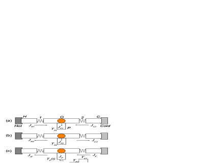
Figure 1: Configuration of the heat pump.

Segment H1 (2C) and 1O2 are coupled to 1 (2) via a spring of constant $k_{1}$ ($k_{2})$. Segments OP and 1O2, which are coupled via the mid-particle of segment O with a spring of constant $k_{3}$, have the same parameters with the exception of the size. The number of the particles in segment 1O2 is nearly twice that in segment OP. The stochastic external force, which is here presented by a heat bath, is applied to modulate the last particle of OP segment. The temperature of the heat bath, $T_{P}(t)$, is a periodic square wave function. As shown in Fig.1c, $T_{P}(t)$ equals to $T_{P1}$ in the first half period and $T_{P2}$ in the second half period, respectively. The total Hamiltonian of the model is

$$H=\overset{M}{\sum}H_{M}+\sum H_{int},$$ (1)

and the Hamiltonian of each segment can be written as

$$H_{M}=\sum_{i=1}^{N_{M}}\left[\frac{p_{M,i}^{2}}{2m_{M}}+\frac{k_{M}}{2}\left(x_{M,i+1}-x_{M,i}\right)^{2}+\frac{V_{M}}{(2\pi)^{2}}\left[1-\cos(2\pi x_{M,i})\right]\right],$$ (2)

with $x_{M,i}$ and $p_{M,i}$ denote the displacement from equilibrium position and the conjugate momentum of the $i^{th}$ particle in segment $M$, where $M$ stands for $H1$, $1O2$, $2C$ or $OP$. $N$ is the number of the particles in segments $H1$, $2C$ and $OP$. The number of the particles in segment $1O2$ is $2N+1$. $\sum H_{int}=H_{1}+H_{2}+H_{3}$, in which $H_{1}=k_{1}\left(x_{H,1}-x_{O,1}\right)^{2}/2$, $H_{2}=k_{2}\left(x_{O,2N+1}-x_{C,1}\right)^{2}/2$, and $H_{3}=k_{2}\left(x_{O,N+1}-x_{P,1}\right)^{2}/2$. We set the masses of all the particles be unit and use fixed boundaries, $x_{W,N+1}=0,$where W stands for H, C, or P. The main parameters are $k_{H1}=1.0$, $k_{2C}=9.0$, $k_{1O2}=k_{OP}=3.0$, $V_{H1}=2.0$, $V_{2C}=4.5$, $V_{1O2}=V_{OP}=3.0$, $k_{1}=k_{2}=0.05$, $\ k_{3}=3.0$, $T_{H}=0.20$, and $T_{C}=0.16$

In our simulations we use Nose-Hoover thermostat Nose and integrate the equations of motion by using the 4th-order Runge-Kutta algorithm Press . We have checked that our results do not depend on the particular thermostat realization (for example, Langevin thermostat). The local temperature is defined as $T_{i}=\left\langle p_{i}^{2}\right\rangle$, $\langle$ $\rangle$ means time average. The local heat flux along the chain is defined as $J_{W,i}=k_{M}\langle p_{i}(x_{i}-x_{i-1})\rangle$, where $W$ stands for $H$, $C$ and $P$. $i$ is the order of the particle. The heat current, which flows from $H$ to $C(J_{H})$, or $O$ to $C(J_{C})$, or $O$ to $P(J_{P})$, is defined as the positive current. The average kinetic energy is $E_{K}=\sum_{i=1}^{4N+1}\langle v_{i}^{2}\rangle/(4N+1)$, where $v_{i}$ is the velocity of the $i^{th}$ particle and $4N+1$ is the system size, respectively. The simulations are performed long enough to allow the system to reach a steady state in which the local heat flux is constant along the chain.

Here the external perturbation has the same effect as a heat bath coupled to the particle in the end of segment $OP$. In our model, Figure 2 shows the temperature of mid-particle of segment $1O2$, $T_{O}$, changes linearly with the temperature of the heat bath acted on segment P. Due to ballistic transport of weak link systems in low temperature WRZhong1 , the temperature of particle $O$ nearly equals to the temperature of the heat bath $T_{P}(t)$ i.e., $T_{O}\approx T_{P}$. As the temperature of the heat bath connects to P is low enough, the temperature of interface particle $O$ ($T_{O}$) is also small. Therefore, when $T_{O}$ is smaller than $T_{H}$ and $T_{C}$, the system absorbs energy from both heat baths and then the direction of the heat current is shown in Fig.1a, here we set the heat current $J_{H1}>0$, $J_{C1}<0$, and $J_{P1}>0$. When $T_{O}$ is larger than $T_{H}$ and $T_{C}$, the energy will dissipate from the system oscillator mode to heat baths and then the direction of the heat current is shown in Fig.1b, here the heat current $J_{H2}<0$, $J_{C2}>0$, and $J_{P2}<0$. The temperature profiles along the configuration of the system is shown in the inset of Fig.2 for $T_{P}=0.02$ and $0.22$. Actually, the temperature of the controlling heat bath is variable. Provided that we use the appropriate values of $T_{P1}$ and $T_{P2}$ and perform the simulation in long time enough (the simulation time is far larger than the relaxation time of the system), as shown in Fig.1c, we will get a negative value of the total heat current in one period, i.e., $J_{H}<0$ and $J_{C}<0$, which means a pumping operation.

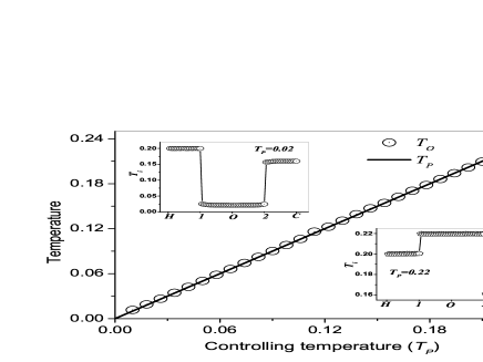
Figure 2: Relationship between the temperature of particle $O$ and the temperature of the controlling heat bath $T_{P}$. The inset is the temperature profiles along segments $H-1-O-2-C$ as shown in Fig.1a for $T_{P}=0.02$ and $0.22$.

This phenomenon can be understood from two essential physical principles: negative differential thermal resistance (NDTR) and thermal rectification (TR) BLi1 BLi2 WRZhong1 . These two effects produce nonlinear relationship between the heat current and the temperature difference. It can be explained in detail as follows:

As shown in Figs.3a, in the region of low temperature ($T_{O}<T_{C}<T_{H})$, when temperature $T_{O}$ is decreased by decreasing the temperature of the controlling heat bath $T_{P}$, $J_{H}$ increases firstly and then decreases to a small value, however, $J_{C}$ decreases linearly. The dependence of $J_{H}$ on the temperature difference $T_{H}-T_{O}$ shows a NDTR effect. In high temperature region ($T_{O}>T_{H}>T_{C})$, $J_{H}$ and $J_{C}$ have linear relationships with the temperature. In a brief, segment $HO$ is in the open state for $T_{O}>T_{H}$ but in the close state for $T_{O}<T_{H}$. This effect is not visible in segment $OC$. If we select two appropriate values of $T_{P}$, $T_{P1}=0.02$ and $T_{P2}=0.22$, as the temperature in the first and the second half period, the total heat currents $J_{H}(J_{H1}+J_{H2})$ and $J_{C}(J_{C1}+J_{C2})$ equal to $-4.30\times 10^{-5}$ and $-1.15\times 10^{-5}$, respectively. Heat pump works on the condition that the negative heat flux is larger than the positive one during a period.

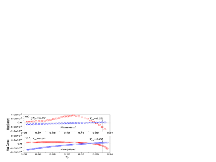
Figure 3: Heat currents through two terminals H ($J_{H}$, red square) and C ($J_{C}$, blue circle) versus the temperature of the controlling heat bath $T_{P}$. (a) Numerical results for the system size 4N+1=65 and (b) analytical results based on Eq.(5).

The corresponding analytical method is also included. As reported in Refs BHu and DHe , we replace the first and second derivatives of the external potential by their thermal average with respect to the effective harmonic Hamiltonian, and then equation 2 can be approximated by self-consistent phonon theory as

$$\overset{\char 126\relax}{H}_{M}=\sum_{i=1}^{N_{M}}\left[\frac{p_{M,i}^{2}}{2}+\frac{k_{M}}{2}\left(q_{M,i+1}-q_{M,i}\right)^{2}+\frac{g_{M}}{2}(q_{M,i})^{2}\right],$$ (3)

in which

$$g_{M}=\frac{V_{M}}{2}\exp\left[-\frac{2\pi T_{M}}{\sqrt{g_{M}(4k_{M}+g_{M})}}\right],$$ (4)

where $T_{M}$ means the average temperature and $M$ refers to segments $HO$, $OC$ and $OP$. Here we solve the transcendental equation 4 through calculating the intersection point of left part and right part of the equation WRZhong2 . As $k_{1}\longrightarrow 0,$ considering classical Landauer-type equation, we can get the heat current flows from $H$ to $O$ as

$$J_{H}=\frac{k_{B}(T_{H}-T_{O})}{2\pi}\int_{\omega_{1}}^{\omega_{2}}\chi(\omega)d\omega,$$ (5)

in which the transmission coefficient is

$$\chi(\omega)\approx\frac{k_{1}^{2}}{k_{H}k_{O}}\sqrt{\frac{(4k_{H}+g_{H}-\omega^{2})(4k_{O}+g_{O}-\omega^{2})}{(\omega^{2}-g_{H})(\omega^{2}-g_{O})}}.$$ (6)

The cutoff frequencies range from $\omega_{1}=\max\{\sqrt{g_{H}},\sqrt{g_{O}}\}$ to $\omega_{2}=\min\{\sqrt{4k_{H}+g_{H}},\sqrt{4k_{O}+g_{O}}\}$, which correspond to the boundaries of the overlap band of left and right phonon spectra. Provided that $T_{H}$ and $T_{O}$ are available, then we can obtain the heat current flows from $H$ to $O$, $J_{H}$. Similarly, as $k_{2}\longrightarrow 0$, we can also get the heat current from $O$ to $C$, $J_{C}$. Due to the linear relationship of $T_{O}$ and $T_{P}$, figure 3b analytically confirms the NDTR and TR effects in T-shape FK lattices, which is numerically presented in Fig.3a.

Heat pump is a dynamical and nonequilibrium effect during macroscopic time. Therefore, heat pump has some valid conditions. We give three main parameters which influence the state of heat pump significantly.

Temperature dependence In order to obtain four heat currents, $J_{H1}$, $J_{H2}$, $J_{C1}$, and $J_{C2}$, shown in Figs.1a and 1b, obviously the temperature $T_{O}$ should satisfy $T_{O}<T_{C}<T_{H}$ in the first half period and $T_{C}<T_{H}<T_{O}$ in the second half period, respectively. Since $T_{O}$ almost equals to $T_{P}$, as illustrated in Fig.2, $T_{P}$ has to satisfy $T_{P}<T_{C}<T_{H}$ in the first half period and $T_{C}<T_{H}<T_{P}$ in the second half period, respectively. Here the main point is what is the range of $T_{P}(t)$. Generally, we fix the low temperature level $T_{P1}(=0.02)$ and change the high temperature level $T_{P2}$. Figure 4 displays that the total heat currents, $J_{H}$ and $J_{C}$, are negative as $T_{P2}$ ranges from 0.210 to 0.303. This range of $T_{P2}$ is defined as pumping region. When $T_{P2}<0.210$ or $T_{P2}>0.303$, pumping effect cannot be realized. It is worth mentioning a point, where $T_{P2}=0.251$ and $J_{H}=J_{C}=-0.51\times 10^{-5}<0$, indicates the optimum pumping.

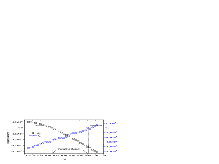
Figure 4: Temperature dependence of the heat current in a T-shape FK lattice. The vibration period of $T_{P}(t)$ is $5.0\times 10^{6}$ steps and the system size is 65.

Frequency dependence In our simulation, the system relaxation time ($\tau_{s}$) of our model is about $6.0\times 10^{9}$ simulation steps, then $\tau_{s}$=$6.0\times 10^{7}$. The oscillating frequency of single particle ($\omega_{p}$, or 1/$\tau_{p}$) ranges from $2.5\times 10^{-3}$ to $6.2\times 10^{-1}$, which can be calculated through the phonon spectral analysis of the particle’s velocity BLi2 . In order to get a stable heat current, the vibration period of temperature level $T_{P}(t)$ should be far smaller than the system relaxation time. Furthermore, the vibration period of noise level cannot be near the oscillating period of single particle. As shown in Fig.5a, in the case of low frequency, the heat pump works normally with a stable negative heat current $J_{H}$. However, when the vibration frequency of temperature is increased to a value larger than $3.0\times 10^{-3}$, the direction of heat current changes and the heat pump stops working. It is easily understood from the change of the average kinetic energy with the frequency. As shown in Fig.5b, the system maintains its average kinetic energy onto a value $E_{K}$ ($=\frac{1}{2}(E(T_{P1})+E(T_{P2}))=0.072$) at low frequency. However, the average kinetic energy has a significant change in the frequency region of single particle, which corresponds to the shadow area in Fig.5. In this region, the frequency may match the oscillating frequency of single particle, the temperature of the controlling heat bath has a significant influence on the oscillating energy of every particle and the system is nonconservative. Therefore, we set the vibration period of temperature level, $\tau_{n}$, be $5.0\times 10^{4}$ , which satisfies $\tau_{p}<<\tau_{n}<<\tau_{s}$.

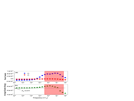
Figure 5: Frequency dependence of (a) heat currents and (b) average kinetic energy of heat pump. The remaining parameters are the same as for Fig.4.

System size effect The results displayed above are for a system with 65(4N+1) particles. Since the heat pump mechanism in our model is due to the coupling between two asymmetric lattices it is reasonable to expect that the system size will definitely influence the heat pump efficiency. As shown in Fig.6, the heat current is dependent on the system size. The heat current of heat pump increases firstly and then decreases by increasing the number of particles. Finally, the heat pump stops working when the system size is larger than 500. This phenomenon can be understood by system size dependence of NDTR WRZhong1 . When the system size is increased, the system goes to completely diffusive transport regime and then NDTR disappears. Thus, the valid condition for heat pump will be unavailable.

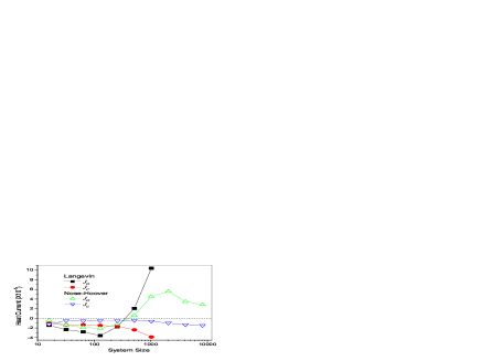
Figure 6: The finite size effect of the pumping efficiency for two kinds of heat baths, Langevin (solid Squares and Circles) and Nose-Hoover (open Up Triangles and Down Triangles). The remaining parameters are $T_{P1}=0.02$, $T_{P2}=0.22$, and $\tau_{n}=5.0\times 10^{6}$.

We have to point out that in this letter we use the more complex four segments rather than three segments FK lattices just for the convenience of theoretical analysis. Actually, in the case of three segment lattices, the heat pump may work more efficiently. Finally, we would like to discuss the improvement of our heat pump model. Figure 1 displays a single heat pump working between two heat baths with small temperature difference. Moreover, this kind of single heat pump works with low pumping efficiency. Therefore, if we expect to get a more powerful heat pump, we can connect single heat pumps in series or in parallel.

Up to now we only pay attention to the behavior of the device as a heat pump, which requires $J_{H}<0$ and $J_{C}<0$; however, for the situation with only $J_{C}<0$ (when the system size is larger than 500 as shown in Fig.6), which would be useful as a refrigerator mode to extract heat from the cold source, although in this case this heat will not go to the hot source but will go to the oscillating heat bath; anyway, the ensemble will globally act as a refrigerator.

In conclusions, we have reported the feasibility to produce molecular heat pump based on T-shape FK model. This device can pump the heat from the low-temperature region to the high-temperature region through controlling the atomic temperature of the third terminal. Although the heat pump presented here is only an ideal model, it can be easily imitated in experiment. The study may also be a valuable illumination in fabricating nanoscale heat pump. Besides, our heat pump model will help deeply understand the effect of negative differential thermal resistance.

- (1) The Systems and Equipment volume of the ASHRAE Handbook, ASHRAE, Inc., Atlanta, GA, (2004).
- (2) A . Nitzan, Science, 317, 759 (2007).
- (3) R. Marathe, A. M. Jayannavar, and A. Dhar, Phys. Rev. E 75, 030103(R) (2007).
- (4) N. Nakagawa and T. S. Komatsu, Europhys. Lett. 75, 22 (2006).
- (5) D. Segal and A. Nitzan, Phys. Rev. E 73, 026109 (2006).
- (6) D. Segal, Phys. Rev. Lett 101, 260601 (2008).
- (7) Y. Wei, L.Wan, B. Wang, and J. Wang, Phys. Rev. B 70, 045418 (2004).
- (8) P. Hanggi and F. Marchesoni, Artificial Brownian motors: Controlling transport on the nanoscale, Rev. Mod. Phys. 81, 1–55 (2009).
- (9) M. Van den Broek and C. Van den Broeck, Phys. Rev. Lett. 100, 130601 (2008).
- (10) B. Li, Lei Wang, and Giulio Casati, Appl. Phys. Lett. 88, 143501 (2006).
- (11) L. Wang, and B. W. Li, Phys. Rev. Lett. 99, 177208 (2007).
- (12) V. Pouthier, J. C. Light, and C. Giraredet, J. Chem. Phys. 114, 4955 (2001).
- (13) Z. L. Wang, Z. W. Pan, and Z. R. Dai, Microsc. Microanal. 8, 467-474 (2002).
- (14) A. Cummings, M. Osman, D. Srivastava, and M. Menon, Phys. Rev. B 70, 115405 (2004).
- (15) S. Nose, J. Chem. Phys. 81, 511 (1984); W. G. Hoover, Phys. Rev.A 31, 1695 (1985).
- (16) W. H. Press, S. A. Teukolsky, W. T. Vetterling, and B. P. Flannery, Numerical Recipes (Cambridge University Press, Cambridge, 1992).
- (17) W. R. Zhong, P. Yang, B. Q. Ai, Z. G. Shao, and B. Hu, Phys. Rev. E 79, 050103 (2009).
- (18) B. Hu, D. He, L. Yang, and Y. Zhang, Phys. Rev. E 74, 060101 (2006).
- (19) D. H. He, Thermal Rectification in One-Dimensional Nonlinear Systems, (PhD Thesis of Hong Kong Baptist University, Hong Kong, 2008).
- (20) W. R. Zhong, Y. Z. Shao, and Z. H. He, Phys. Rev. E 74, 011916 (2006).