Energy spectra of three electrons in Si/SiGe single and vertically coupled double quantum dots

Abstract

We study three-electron energy spectra in Si/SiGe single and vertically coupled double quantum dots where all the relevant effects, such as, the Zeeman splitting, spin-orbit coupling, valley coupling and electron-electron Coulomb interaction are explicitly included. In the absence of magnetic field, our results in single quantum dots agree well with the experiment by Borselli et al. [Appl. Phys. Lett. 98, 123118 (2011)]. We identify the spin and valley configurations of the ground state in the experimental cases and give a complete phase-diagram-like picture of the ground state configuration with respect to the dot size and valley splitting. We also explicitly investigate the three-electron energy spectra of the pure and mixed valley configurations with magnetic fields in both Faraday and Voigt configurations. We find that the ground state can be switched between doublet and quartet by tuning the magnetic field and/or dot size. The three-electron energy spectra present many anticrossing points between different spin states due to the spin-orbit coupling, which are expected to benefit the spin manipulation. We show that the negligibly small intervalley Coulomb interaction can result in magnetic-field independent quartet-doublet degeneracy in the three-electron energy spectrum of the mixed valley configuration. Furthermore, we study the barrier-width and barrier-height dependences in vertically coupled double quantum dots with both pure and mixed valley configurations. Similar to the single quantum dot case, anticrossing behavior and quartet-doublet degeneracy are observed.

I INTRODUCTION

Silicon quantum dots (QDs) are proposed to be prominent candidates for spin qubits owing to the long spin-decoherence time,Loss1 ; Reimann1 ; Hanson2 ; Wu_rev ; Eriksson1 ; Berezovsky1 ; Harju1 ; Dimi1 ; Dimi2 ; Lwang1 ; Lwang2 ; Dimi3 ; Tahan1 which is of great importance for coherent manipulation, information storage and quantum error correction.Tahan1 ; Shor1 ; Sherwin1 ; Cory1 ; Bennett1 The long decoherence time in Si-based devices results from the weak hyperfine interaction,Lwang1 small spin-orbit coupling (SOC)Dresselhaus1 ; Vervoort1 ; Vervoort2 ; Rashba1 ; Bockelmann1 ; Landolt1 ; Nestoklon1 and weak electron-phonon interaction.Li1 As an indirect-gap semiconductor, the conduction band of the bulk Si has six degenerate minima or valleys. This six-fold degeneracy can be lifted by strain or quantum confinement, e.g., it separates into a four-fold degeneracy and a two-fold one in [001] quantum wells. The two-fold degenerate valleys with low energy can be further lifted by a valley splitting due to the interface scattering.Friesen1 ; Ando1 The existence of the valley degree of freedom makes the Si-based qubits more attractive.Dimi1 ; Dimi2 ; Lwang1 ; Lwang2 ; Dimi3 Moreover, the mature microfabrication technology of the classical Si-based electronics is proposed to benefit the realization of Si spin qubits.Dimi1 ; Lwang1

Recently, Si quantum dots (QDs) have been widely investigated both experimentally and theoretically.Harju1 ; Eriksson1 ; Borselli1 ; Xiao1 ; Lim1 ; Lim2 ; Fabian1 ; Dimi1 ; Dimi2 ; Dimi3 ; Lwang1 ; Lwang2 ; Barnes1 In the experiments, Si metal-on-semiconductor and Si/SiGe QDs with a tunable electron filling number from zero have been fabricated, where the valley splitting, few-electron energy spectrum and spin relaxation time have been measured.Borselli1 ; Xiao1 ; Lim1 ; Lim2 The theoretical works mainly focus on the one-electron Zeeman sublevels or the singlet-triplet states of two electrons.Harju1 ; Eriksson1 ; Fabian1 ; Dimi1 ; Dimi2 ; Dimi3 ; Lwang1 ; Lwang2 For example, Culcer et al.Dimi1 ; Dimi2 ; Dimi3 analyzed the initialization and manipulation of one-electron and two-electron qubits in lateral coupled double quantum dots (DQDs) by utilizing the valley degree of freedom. Raith et al.Fabian1 calculated the energy spectrum and the spin relaxation time in one-electron QDs. By explicitly including the electron-electron Coulomb interaction, Wang et al. obtained the two-electron spectrum from exact-diagonalization method and calculated the singlet-triplet relaxation time in both singleLwang1 and lateral coupled doubleLwang2 QDs. As pointed out by Barnes et al.,Barnes1 the robustness of the quantum states against charge impurity and noise in QDs can be improved by increasing the number of the electrons, which reveals the necessity of the theoretical investigation on multi-electron spin qubits. The energy spectra in multi-electron GaAs QDs have been explicitly calculated to identify the specific spin configuration of each state, where only one valley is relevant.GaAs1 ; GaAs2 ; GaAs3 ; GaAs4 ; Gamucci1 However, to the best of our knowledge, there is no report on the explicit calculation in silicon QDs with three or more electrons due to the complication of the calculation. Alternatively, Hada et al.Hada1 neglected the correlation effect and calculated the three-electron energy spectrum within single configuration approximation in single QDs. However, the correlation effect has been shown to present significant influence on the energy spectrum via strong Coulomb interaction in Si QDs.Lwang1 ; Hada1 ; Eto1 Therefore, in order to obtain the accurate convergent spectrum, the exact-diagonalization method with sufficient basis functions is required. The goal of the present work is to analyze the energy spectrum in the three-electron Si/SiGe QDs based on the exact-diagonalization method.

In this work, we calculate the three-electron energy spectrum in both single and vertically coupled double QDs with the Zeeman splitting, SOC, valley coupling and electron-electron Coulomb interaction explicitly included. In the single dot case, we first calculate the ground state energy in the absence of the magnetic field, where good agreement with the experimental data is achieved. Our calculation also uncovers the valley and spin configurations of the ground state in experiment. We present a complete phase-diagram-like picture to describe the spin and valley configurations of the ground state. We find that the ground state is of pure (mixed) valley configuration at large (small) valley splitting. The spin configuration of the ground state can be controlled through dot size for the pure valley configuration, while that in the mixed valley configuration is always doublet. The magnetic field dependence of the three-electron energy spectrum in each “phase” is investigated. We take into account both orbital effect and Zeeman splitting for the perpendicular magnetic field and only Zeeman splitting for the parallel magnetic field owing to the strong confinement along the growth direction. We find that the spin configuration of the ground state can also be switched by magnetic field. For the mixed valley configuration, we find interesting quartet-doublet degeneracy, which results from the negligibly small intervalley interaction. In the DQD case, the barrier-width and barrier-height dependences of the energy spectrum with both pure and mixed valley configurations are discussed. Moreover, we show many anticrossing points resulting from the SOCs in all cases.

This paper is organized as follows. In Sec. II, we set up our model and formalism. In Sec. III, we show our results of the three-electron energy spectrum in single QDs and vertically coupled DQDs from the exact-diagonalization method. We investigate the perpendicular and parallel magnetic-field dependences in single QDs and the barrier-width and barrier-height dependences in vertically coupled DQDs. The comparison with experiment in single QD case is also given in this section. Finally, we summarize in Sec. IV.

II MODEL AND FORMALISM

We set up our model in a double quantum well along [001]-direction. The confinement along this direction is described byYYWang1 ; Shen1

$$V_{z}(z) = \left\{\begin{array}[]{cc}V_{0},&\mbox{$|z|<\tfrac{a}{2}$},\\[3.0pt] 0,&\mbox{$\tfrac{a}{2}\leq|z|\leq\tfrac{a}{2}+d$},\\[3.0pt] \infty,&\mbox{$\rm otherwise$},\end{array}\right.$$ (4)

with the inter-well barrier height denoting as $V_{0}$. Here, $d$ and $a$ represent the width of each well and that of the barrier, respectively. The lateral confinement is chosen to be a parabolic potential $V_{\rm c}(x,y)=\tfrac{1}{2}m_{t}\omega_{0}^{2}(x^{2}+y^{2})$ with $m_{t}$ representing the in-plane effective mass and $\omega_{0}$ being the confining potential frequency.Fock1 ; Darwin1 The effective diameter $d_{0}$ is given by $\sqrt{\hbar\pi/(m_{t}\omega_{0})}$. The total confinement potential then can be written as $V(\mathbf{r})=V_{\rm c}(x,y)+V_{z}(z)$. For an infinitesimal barrier width ($a\sim 0$), our model reduces to the single dot case.

The external magnetic field with perpendicular and parallel components is expressed by ${\mathbf{B}}=B_{\perp}\hat{\mathbf{z}}+B_{\parallel}\hat{\mathbf{x}}$. The single-electron Hamiltonian readsLwang1

$$H_{\rm e}=\frac{P_{x}^{2}+P_{y}^{2}}{2m_{t}}+\frac{P_{z}^{2}}{2m_{z}}+V(\mathbf{r})+H_{\rm Z}+H_{\rm so}+H_{\rm v},$$ (5)

where $m_{z}$ denotes the effective mass along the growth direction and ${\mathbf{P}}=-i\hbar{\mbox{\boldmath$\nabla$\unboldmath}}+(e/c){\mathbf{A}}$ with the vector potential ${\mathbf{A}}=(-yB_{\perp},xB_{\perp},2yB_{\parallel})/2$. In our calculation, the orbital effect of the parallel component of the magnetic field is neglected due to the strong confinement along the $z$-direction and the vector potential in the mechanical momentum then reduces to ${\bf A}=(-yB_{\perp},xB_{\perp},0)/2$. In Eq. (5), the Zeeman splitting is given by $H_{\rm Z}=\tfrac{1}{2}g\mu_{B}(B_{\perp}\sigma_{z}+B_{\parallel}\sigma_{x})$ with $g$ being the Land$\acute{\rm e}$ factor. The SOCs, including the Rashba termRashba1 due to the structure inversion asymmetry (SIA) and the interface-inversion asymmetry (IIA) term,Vervoort2 ; Vervoort1 ; Nestoklon1 are expressed by

$$H_{\rm so}=a_{0}(P_{x}\sigma_{y}-P_{y}\sigma_{x})+b_{0}(-P_{x}\sigma_{x}+P_{y}\sigma_{y}),\mbox{}$$ (6)

where $a_{0}$ ($b_{0}$) represents the coupling coefficient of the Rashba (IIA) term. $H_{\rm v}$ in Eq. (5) describes the coupling between the two low-energy valleys lying at $\pm\langle k_{\rm Si}\rangle$ along the $z$-axis with $\langle k_{\rm Si}\rangle=0.85(2\pi/a_{\rm Si})$.Friesen1 Here, $a_{\rm Si}=5.43\;{\rm\AA}$ stands for the lattice constant of silicon. In this work, we use “$z$” (“$\overline{z}$”) to denote the valley lying at $\langle k_{\rm Si}\rangle$ ($-\langle k_{\rm Si}\rangle$) for convenience.

In order to build up a complete set of single-electron basis functions, we define $H^{\prime}_{0}=H_{0}+H_{\rm v}$ with $H_{0}=\tfrac{P_{x}^{2}+P_{y}^{2}}{2m_{t}}+\tfrac{P_{z}^{2}}{2m_{z}}+V(\mathbf{r})$. Due to the separation of the lateral and vertical confinement, one can easily solve the Schrödinger equation of $H_{0}$. From the lateral part, one obtains the eigenvaluesCheng1 ; Fock1 ; Darwin1

$$E_{nl}=\hbar\Omega(2n+|l|+1)+\hbar l\omega_{B},\mbox{}$$ (7)

where $\Omega=\sqrt{\omega_{0}^{2}+\omega_{B}^{2}}$ and $\omega_{B}=eB_{\perp}/(2m_{t})$. The eigenfunctions readCheng1 ; Fock1 ; Darwin1

$$K_{nl}(r,\theta)=N_{n,l}(\alpha r)^{|l|}e^{-(\alpha r)^{2}/2}e^{il\theta}L_{n}^{|l|}[(\alpha r)^{2}],\mbox{}$$ (8)

with $N_{n,l}=\{\alpha^{2}n!/[\pi(n+|l|)!]\}^{1/2}$ and $\alpha=\sqrt{m_{t}\Omega/\hbar}$. $L^{|l|}_{n}$ is the generalized Laguerre polynomial. Here, $n=0,1,2,...$ is the radial quantum number and $l=0,\pm 1,\pm 2,...$ is the azimuthal angular momentum quantum number. For the vertical part, we include the lowest two subbands, one with even parity (denoted by subscript $n_{z}=0$) and the other with odd parity ($n_{z}=1$). The corresponding wave functions can be expressed asShen1

$$\xi_{0}(z) = \left\{\begin{array}[]{ccccccc}C_{0}\sin[k_{0}(z-\tfrac{a}{2}-d)],&\mbox{$\tfrac{a}{2}\leq z\leq\tfrac{a}{2}+d$},\\[3.0pt] A_{0}\cosh(\beta_{0}z),&\mbox{$|z|<\frac{a}{2}$},\\[3.0pt] C_{0}\sin[k_{0}(-z-\tfrac{a}{2}-d)],&\mbox{$-\tfrac{a}{2}-d\leq z\leq-\tfrac{a}{2}$},\\[3.0pt] 0,&\mbox{otherwise},\\ \end{array}\right.$$ (10)

and

$$\xi_{1}(z) = \left\{\begin{array}[]{ccccccc}C_{1}\sin[k_{1}(z-\tfrac{a}{2}-d)],&\mbox{$\tfrac{a}{2}\leq z\leq\tfrac{a}{2}+d$},\\[3.0pt] A_{1}\sinh(\beta_{1}z),&\mbox{$|z|<\tfrac{a}{2}$},\\[3.0pt] C_{1}\sin[k_{1}(z+\tfrac{a}{2}+d)],&\mbox{$-\tfrac{a}{2}-d\leq z\leq-\tfrac{a}{2}$},\\[3.0pt] 0,&\mbox{otherwise},\\ \end{array}\right.$$ (13)

with $k_{n_{z}}=\sqrt{2m_{z}E_{n_{z}}/\hbar^{2}}$ and $\beta_{n_{z}}=\sqrt{2m_{z}(V_{0}-E_{n_{z}})/\hbar^{2}}$. $E_{n_{z}}$ is the eigenvalue of the $n_{z}$-th subband. For the single dot case, only the lowest subband ($n_{z}=0$) is relevant. With the knowledge of the eigenfunctions of $H_{0}$, one expresses the single-electron basis functions in different valleys as $\phi^{z(\overline{z})}_{nln_{z}}=K_{nl}\xi_{n_{z}}e^{\pm ik_{\rm Si}z}u_{z(\overline{z})}({\mathbf{r}})$, with $u_{z(\overline{z})}(\mathbf{r})$ being the lattice-periodic Bloch functions.

Then we introduce the valley coupling $H_{\rm v}$ according to Ref. Friesen1, , where the relevant components are given byDimi1 ; Lwang1 $\langle\phi^{z}_{n^{\prime}l^{\prime}n_{z}}|H_{\rm v}|\phi^{z}_{nln_{z}}\rangle=\langle\phi^{\overline{z}}_{n^{\prime}l^{\prime}n_{z}}|H_{\rm v}|\phi^{\overline{z}}_{nln_{z}}\rangle=\Delta^{0}_{n_{z},n_{z}}\delta_{n,n^{\prime}}\delta_{l,l^{\prime}}$ and $\langle\phi^{z}_{n^{\prime}l^{\prime}n_{z}^{\prime}}|H_{\rm v}|\phi^{\overline{z}}_{nln_{z}}\rangle=\langle\phi^{\overline{z}}_{n^{\prime}l^{\prime}n_{z}^{\prime}}|H_{\rm v}|\phi^{z}_{nln_{z}}\rangle=\Delta^{1}_{n_{z},n_{z}^{\prime}}\delta_{n,n^{\prime}}\delta_{l,l^{\prime}}$. The expressions of $\Delta^{0}_{n_{z},n_{z}}$ and $\Delta^{1}_{n_{z},n_{z}^{\prime}}$ are given in Appendix A. Since the valley coupling between different subbands ($n_{z}\neq n_{z}^{\prime}$) in our case is much smaller than the intersubband energy difference ($<2$ %), we neglect the intersubband valley coupling. The eigenstates of $H_{0}^{\prime}$ then can be written as $\phi^{\pm}_{nln_{z}}=\tfrac{1}{\sqrt{2}}(\phi^{z}_{nln_{z}}\pm\phi^{\overline{z}}_{nln_{z}})$ and the corresponding eigen-energies are $E^{\pm}_{nln_{z}}=E_{nl}+E_{n_{z}}+E^{\pm}_{n_{z}}$. with $E^{\pm}_{n_{z}}=\Delta^{0}_{n_{z},n_{z}}\pm|\Delta^{1}_{n_{z},n_{z}}|$ representing the energy from the valley degree of freedom and $\Delta E^{\rm v}_{n_{z}}=2|\Delta^{1}_{n_{z},n_{z}}|$ being the valley splitting.

For the three-electron case, the total Hamiltonian can be expressed as

$$H_{\rm tot} = H^{1}_{\rm e}+H^{2}_{\rm e}+H^{3}_{\rm e}+H^{12}_{\rm C}+H^{23}_{\rm C}+H^{13}_{\rm C}.\mbox{}$$ (15)

The superscripts “1”, “2” and “3” on the right hand side of the equation label the relevant electrons, e.g., $H^{i}_{\rm e}$ represents the single-electron Hamiltonian of the $i$-th electron given by Eq. (5) and $H^{i,j}_{C}=\tfrac{e^{2}}{4\pi\varepsilon_{0}\kappa|{\mathbf{r}_{i}}-{\mathbf{r}_{j}}|}$ stands for the Coulomb interaction between $i$-th and $j$-th electrons. Here, $\kappa$ is the relative static dielectric constant.

By using the single-electron functions {$\phi^{\pm}_{nln_{z}}$} or $\{|nln_{z}n_{{\rm v}}\rangle\}$ ($n_{\rm v}=\pm$ denotes the valley eigenfunction), we construct the three-electron basis functions in the form of either doublet ($S_{\rm tot}=\frac{1}{2}$, denoted as $|D^{(\Xi)}_{S^{*}}\rangle$) or quartet ($S_{\rm tot}=\frac{3}{2}$, denoted as $|Q^{(\Xi)}_{S^{*}}\rangle$) with Clebsch-Gordan coefficients. Subscript $S^{*}$ stands for the spin magnetic quantum number. Superscript $\Xi$ denotes four valley configurations of three-electron basis functions, i.e. $\Xi=-(+)$ for the case three electrons in “$-$” (“$+$”) valley and $\Xi={\rm m}$ ($\widetilde{\rm m}$) for two electrons in “$-$”(“$+$”) valley and one electron in “$+$”(“$-$”) valley. The details of the three-electron basis functions are given in Appendix B.

One calculates the matrix elements of Eq. (15) under the three-electron basis functions. The details of the Coulomb interaction are given in Appendix C. By neglecting the small coupling between basis functions of different valley configurations,Dimi1 ; Lwang1 the complete basis functions can be divided into four individual sets according to valley configurations ($\Xi=-$, ${\rm m}$, $\widetilde{\rm m}$ and $+$). We diagonalize the Hamiltonian of each subspace and define an eigenstate as doublet $|D^{(\Xi)}_{S^{*}}\rangle$ (quartet $|Q^{(\Xi)}_{S^{*}}\rangle$) if its amplitude of doublet (quartet) components is greater than $50$ $\%$. In the following, we still use the notations $|D^{(\Xi)}_{S}\rangle$ and $|Q^{(\Xi)}_{S}\rangle$ to describe the spin properties of the eigenstates without any confusion.

III NUMERICAL RESULTS

In our calculation, the effective mass $m_{t}=0.19m_{0}$ and $m_{z}=0.98m_{0}$ with $m_{0}$ representing the free electron mass.Dexter1 The strengths of the SOCs between the states with the same valley index “$\pm$” are taken as $a_{0}=\pm 6.06$ m/s and $b_{0}=\pm 30.31$ m/s (Ref. Nestoklon1, ). The Landé factor $g=2$ (Ref. Graefi1, ) and the relative static dielectric constant $\kappa=11.9$ (Ref. Hada1, ). In single QDs, we take 1430 quartets and 3330 doublets to guarantee the convergence of the energy spectrum, while in vertically coupled DQDs we take 7316 quartets and 16008 doublets correspondingly.

III.1 Single quantum dots

III.1.1 Comparison with experiment

Recently, Borselli et al. investigated four Si/SiGe single QDs, which are labeled as Si1, Si2, Si3 and Si4 separately, in the absence of the magnetic field.Borselli1 They measured the tuning voltages for the injection of an additional electron into the QDs, i.e., $\Delta V^{N_{\rm e}}_{G}=V_{G}^{N_{\rm e}\leftrightarrow(N_{\rm e}+1)}-V_{G}^{(N_{\rm e}-1)\leftrightarrow N_{\rm e}}$, where $V^{N_{\rm e}\leftrightarrow(N_{\rm e}+1)}_{G}$ represents the gate voltage where the electron number changes between $N_{\rm e}$ and $N_{\rm e}$+1. Then the addition energy of an incoming electron was determined by $\Delta\mu_{N_{\rm e}}=\mu_{N_{\rm e}+1}-\mu_{N_{\rm e}}=\alpha\Delta V^{N_{\rm e}}_{G}$, where $\mu_{N_{\rm e}}=E^{N_{\rm e}}_{\rm Tot}-E^{N_{\rm e}-1}_{\rm Tot}$ with $E^{N_{\rm e}}_{\rm Tot}$ and $\alpha$ being the total energy of the $N_{\rm e}$-electron ground state and the energy-voltage conversion factor. The experimental data of $\Delta\mu_{1}$ and $\Delta\mu_{2}$ of the four samples (noted with the superscript $\ast$) are listed in Table 1.

	Si1	Si2	Si3	Si4
$\Delta E^{\rm v}_{0}$ (meV)	0	0	0.27	0.12
$d$ (nm)	3.945	3.945	3.945	3.926
$\Delta\mu^{*}_{1}$ (meV)	4.520	3.800	3.916	4.680
$\Delta\mu_{1}$ (meV)	4.452	3.828	4.008	4.671
$R_{1}$ (%)	1.5	0.7	2.3	0.2
$\Delta\mu^{*}_{2}$ (meV)	3.226	2.863	3.146	3.594
$\Delta\mu_{2}$ (meV)	3.318	2.824	3.061	3.613
$R_{2}$ (%)	2.9	1.4	2.7	0.5
$d_{0}$ (nm)	31.5	35.3	34.1	30.3
$\Xi$	${\rm m/\widetilde{m}}$	${\rm m/\widetilde{m}}$	$-$	${\rm m}$
$S_{\rm tot}$	$1/2$	$1/2$	$3/2$	$1/2$
Deg.	4	4	4	2

Table 1: The comparison between experimental dataBorselli1 and our results in four devices, Si1-Si4. $\Delta E^{\rm v}_{0}$ and $d$ are the valley splitting and half-well width used in the calculation. $\Delta\mu_{i}^{*}$ represent the experimental addition energy and $\Delta\mu_{i}$ stand for the theory results. $R_{i}$ stand for the relative error between $\Delta\mu_{i}^{*}$ and $\Delta\mu_{i}$. The effective diameter $d_{0}$ is determined from our calculation.square1 The valley index $\Xi$ denotes valley configuration of three-electron ground state in each sample. $S_{\rm tot}$ and “Deg.” represent the total spin and degeneracy factor of the three-electron ground state in each sample, respectively.

For a theoretical study, one can obtain the total energy of multi-electron ground states and calculate the addition energy. However, the well widths and effective diameters required for quantitative calculation are unavailable in Ref. Borselli1, . Therefore, we first derive the well widths from Eq. (18) with the reference value suggested by the experimental work ($d\sim 4$ nm).width For Si3 and Si4, we use the valley splittings $\Delta E^{\rm v}_{0}$ from the experiment.Borselli1 Since the valley splittings of Si1 and Si2 are too small to be measured in experiment,Borselli1 we take them to be zero in our calculation. Then, we calculate the ground state energies of one-, two- and three-electron cases by treating $d_{0}$ as a parameter and determine its value by the least square method of $\Delta\mu_{1}$ and $\Delta\mu_{2}$.square1 In the previous section, we only introduce the frame of the three-electron case. For the one-electron case, one needs to diagonalize the single-electron Hamiltonian $H_{e}$ as given in Eq. (5), while for the two-electron case we follow the frame in Ref. Lwang1, .

Our results of addition energies as well as the effective diameters of QDs are listed in Table 1. Good agreement with experimental data can be observed for all devices with the largest relative error less than 3 %, which confirms the validity and accuracy of our model. In fact, one can also estimate the effective diameter of the QDs solely from the fitting of $\Delta\mu_{1}$ with the experimental value $\Delta\mu_{1}^{\ast}$. With the effective diameter obtained in this way, we recalculate $\Delta\mu_{2}$ and find that the value also agrees well with $\Delta\mu_{2}^{\ast}$ (within 4 %). We should point out that the Coulomb interaction here is very important in these quantum systems. Without explicitly including the Coulomb interaction, the addition energy is mainly from the orbital energy and the theoretical results become far away from the experimental data.

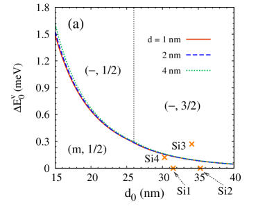
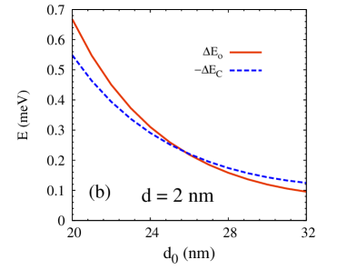
Figure 1: (Color online) (a) Valley and spin configurations of the ground state in the absence of magnetic field. The curves represent the effective diameter dependence of the valley splitting energy for the emergence of the degeneracy between the lowest levels with “$-$” and “m” valley configurations. For each half-well width $d$, the ground state is of “$-$” (“m”) configuration above (below) the corresponding curve. The “$-$”-configuration regime is separated into two parts by the vertical dotted line, according to the total spin $S_{\rm tot}$. The valley configuration and the total spin are labeled as ($\Xi$, $S_{\rm tot}$) in each regime. The crosses represent the parameters in Si1-Si4 in Ref. Borselli1, . (b) The orbital energy difference and the inverse number of Coulomb energy difference between the lowest quartet and doublet states with “$-$” valley configuration vs. effective diameter for $d=2$ nm in the absence of the magnetic field.

III.1.2 Ground state configuration

In Table 1, the valley configuration and total spin of the three-electron ground states are also listed. As shown in the table, the ground state in Si3 is mainly comprised of the quartets with “$-$” valley configuration due to the large valley splitting. This level is four-fold degenerate. However, the valley splitting in Si4 is small and the ground state is two-fold degenerate doublet of “m”-configuration. For Si1 and Si2, the states with “$\widetilde{\rm m}$” valley configuration are degenerate with those with “m”-configuration. Therefore, the ground states are four-fold degenerate. Since the states with different valley configurations are decoupled as mentioned above,Dimi1 ; Lwang1 we explicitly investigate the three-electron spectrum for each valley configuration individually in the following. The relative position between the spectra of different valley configurations is only determined by the exact value of the valley splitting in real system, which is also the criterion of the ground state configuration.

To elucidate the valley and spin configurations of the ground state in the absence of the magnetic field, we draw a phase-diagram-like picture, Fig. 1(a), by calculating the energy difference $\Delta E_{g}^{\rm v}$ between the lowest level with pure (“$-$”) configuration and that with mixed (“m”) configuration. From this figure, one finds three regimes for each half-well width $d$, as labeled by ($\Xi$, $S_{\rm tot}$). It is seen that the ground state is of “$-$” (“m”) valley configuration with large (small) valley splitting as expected. For the “$-$”-configuration case, the ground state can vary between quartet and doublet as the dot size changes, with the transition occurring at around $d_{0}=26$ nm (shown as the vertical dotted line). Since the energy of the lowest “$+$” (“$\widetilde{\rm m}$”) configuration state is always higher than that of the lowest “$-$” (“m”) configuration one due to a finite valley splitting, the ground state can not be of this configuration. However, when $\Delta E^{\rm v}_{0}=0$, the lowest “$\widetilde{\rm m}$”-configuration level is degenerate with “m”-configuration one, therefore, can also be the ground state in that case.

In our calculation, we determine the borderline between different valley configurations from the degenerate condition between them. Specifically, we calculate the energy of the lowest “$-$” and “m” levels in the absence of the valley splitting, i.e., $E^{\rm p}_{\rm g}$ and $E^{\rm m}_{\rm g}$ separately, and obtain $\Delta E^{\rm v}_{\rm g}=E^{\rm p}_{\rm g}-E^{\rm m}_{\rm g}-\Delta E^{\rm v}_{0}$. The valley splitting on the borderline is then given by $\Delta\widetilde{E}^{\rm v}_{0}=E^{\rm p}_{\rm g}-E^{\rm m}_{\rm g}$. Actually, the real value of the valley splitting $\Delta E_{0}^{\rm v}$ for certain well width $d$ should be determined by $\Delta_{0,0}^{1}$ in Appendix A. If the coordinate $(d_{0},\Delta E_{0}^{\rm v})$ locates above the curve of the corresponding well width, i.e., $\Delta E_{0}^{\rm v}>\Delta\widetilde{E}^{\rm v}_{0}$ or $\Delta E^{\rm v}_{\rm g}<0$, the ground state is of “$-$” valley configuration. Otherwise, it should be of “m”-configuration.

The origination of the variation of the ground state spin configuration in the “$-$”-configuration regime is found to be the competition between the orbital and Coulomb energies. The relative orbital (Coulomb) energy between the lowest quartet and doublet $\Delta E_{\rm o}$ ($\Delta E_{C}$) is defined as the orbital (Coulomb) energy of the lowest quartet subtracting that of lowest doublet. One calculates the orbital energy from the expectation of $\sum_{i=1}^{3}H_{e}^{i}$ of the three-electron eigenstates, while the Coulomb energy is similarly given by $H_{C}^{12}+H_{C}^{13}+H_{C}^{23}$. From the explicit expressions of the quartet and doublet given in Appendix B, one notices that all three electrons in quartet must occupy different orbits while two electrons in doublet can stay in the same one. Therefore, the lowest quartet states have higher orbital energy than the lowest doublet states ($\Delta E_{\rm o}>0$). We finds that the Coulomb interaction of the lowest quartet states is smaller than that of the lowest doublet states ($\Delta E_{C}<0$). In Fig. 1(b), we plot $\Delta E_{\rm o}$ and $-\Delta E_{C}$ as function of effective diameter, where an intersecting between these two quantities can be seen. As a qualitative understanding, $\Delta E_{\rm o}\propto 1/d^{2}_{0}$ can be characterized from $\hbar\omega_{0}=\hbar^{2}\pi/(m_{t}d^{2}_{0})$, while $\Delta E_{C}\propto 1/d_{0}$ is estimated from $e^{2}/(4\pi\epsilon_{0}\kappa d_{0})$. Therefore, the orbital energy is more sensitive to the diameter than the Coulomb interaction. For a small diameter QD, the relative position between the lowest doublet and quartet is dominated by the orbital energy and the ground state is doublet. As $d_{0}$ increases, $\Delta E_{\rm o}$ can become smaller than $-\Delta E_{C}$ with the crossover at $d_{0}\sim 26$ nm in Fig. 1(b), resulting in the transition of the ground state from doublet to quartet.

From Fig. 1(a), one can directly read the ground state configuration with the knowledge of the dot size and valley splitting, e.g., Si1-Si4 shown as crosses. Moreover, one notices that our phase-diagram-like picture is robust against the well width, resulting from the strong confinement regime along $z$-direction ($d\ll d_{0}$).

III.1.3 Three-electron spectrum with “$-$” valley configuration

In this part, we take advantage of our model to calculate the three-electron energy spectrum with “$-$”-valley configuration. We study the perpendicular magnetic field dependence at $d=2.12$ nm (corresponding to $\Delta E_{0}^{\rm v}\approx 1.9$ meV) with $d_{0}=20$ nm and $29$ nm, where the ground states lie in the $(-,1/2)$ and $(-,3/2)$ configuration regimes, respectively. The lowest few energy levels are plotted as function of $B_{\perp}$ in Fig. 2. These eigenstates are denoted as $Q^{(-)}_{-3/2}$, $Q^{(-)}_{-1/2}$, $Q^{(-)}_{1/2}$, $Q^{(-)}_{3/2}$, $D^{(-)}_{-1/2}$ and $D^{(-)}_{1/2}$, according to the total spin $S_{\rm tot}$ and $S_{z}$ of the major components in these states. The lowest doublet (quartet) states at $B_{\perp}=0$ T are labeled as circle (open triangle). It is seen that the ground state for $d_{0}=20$ nm is four-fold degenerate doublet, while that for $d_{0}=29$ nm is quartet, consistent with Fig. 1(a). As the magnetic field increases, the degeneracy is lifted due to the effect of the magnetic field on Landau level and Zeeman splitting, resulting in many intersecting points as shown in Fig. 2(a) and (b). We find that some intersecting points show anticrossing behavior due to the SOCs.Lwang1 In this work, all the anticrossing points are labeled by open squares. In the inset, we enlarge the spectrum in the vicinity of one anticrossing point at $B_{\perp}\sim 0.72$ T, where an energy gap $\sim 0.24$ $\mu$eV is present.Rashba1 ; Vervoort1 ; Vervoort2 As reported, the anticrossing points are important for spin manipulation, due to the strong spin mixed at these points.Petta1 ; Nowack1 ; Sarkka1 ; Laird1 ; Petta2 ; Lwang1 ; Lwang2

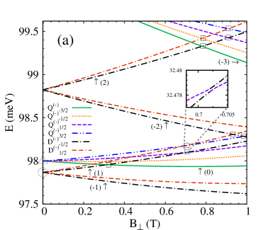
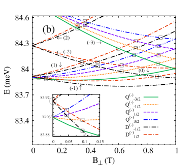
Figure 2: (Color online) The lowest few energy levels vs. perpendicular magnetic field $B_{\perp}$ in single QDs with $d=2.12$ nm and the effective diameter $d_{0}=20$ nm (a) and 29 nm (b). The anticrossing points are labeled by open squares. The circle and open triangle at $B_{\perp}=0$ describe the lowest doublet and quartet states separately. The total orbital angular momentum $L=l_{1}+l_{2}+l_{3}$ of the energy level are labeled correspondingly.orbit The inset in (a) zooms the vicinity of the anticrossing point at $B_{\perp}\sim 0.72$ T. The inset in (b) enlarges the spectrum in the vicinity of $B\sim 0$ T.

Since the eigenstates are strongly mixed, e.g., the largest component in the ground states is usually in the order of 20%, one can not naively describe an eigenstate by a single basis function. However, away from the anticrossing points, the SOCs are weak and the total orbital angular momentum $L=l_{1}+l_{2}+l_{3}$ is still a good quantum number. In Fig. 2(a), we labeled this quantum number for each state. With this quantum number, one can understand why an intersecting point is anticrossing or not in the presence of SOCs. By rewriting the SOCs in the form of ladder operators, one obtains $H_{\rm so}=\tfrac{2ia_{0}}{\hbar}(P^{+}S^{-}-P^{-}S^{+})-\tfrac{2b_{0}}{\hbar}(P^{+}S^{+}+P^{-}S^{-})$ with $P^{\pm}=(P_{x}\pm iP_{y})/2$ and $S^{\pm}=S_{x}\pm iS_{y}$. Since $P^{\pm}$ ($S^{\pm}$) changes $L$ ($S_{z}$) by one unit, the states with ($L$, $S_{z}$) can only couple with the states with ($L\mp 1$, $S_{z}\pm 1$) via Rashba term and those with ($L\pm 1$, $S_{z}\pm 1$) via IIA term.Lwang1 For example, in the inset of Fig. 2(a), the spin-down doublet with ($1$, $-\tfrac{1}{2}$) (black chain curve) couples with the quartet with ($0$, $\tfrac{1}{2}$) (purple dashed curve) via IIA term, resulting in the anticrossing behavior.

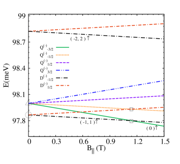
Figure 3: (Color online) The lowest few energy levels vs. parallel magnetic field $B_{\parallel}$ in single QDs. Open squares indicate the anticrossing points. The circle and open triangle at $B_{\perp}=0$ describe the lowest doublet and quartet in the absence of the magnetic field. The total orbital angular momentum $L=l_{1}+l_{2}+l_{3}$ are labeled. The half-well width $d=2.12$ nm and the effective diameter $d_{0}=20$ nm.

To exclude the orbital effect, we apply a parallel magnetic field instead. The results with $d=2.12$ nm and $d_{0}=20$ nm are shown in Fig. 3, where the eigenstates are denoted as $Q^{(-)}_{-3/2}$, $Q^{(-)}_{-1/2}$, $Q^{(-)}_{1/2}$, $Q^{(-)}_{3/2}$, $D^{(-)}_{-1/2}$ and $D^{(-)}_{1/2}$ according to $S_{\rm tot}$ and the $x$-direction component $S_{x}$ of their major components. In this case, the energy levels are linearly dependent on the magnetic field due to the Zeeman splitting. The degeneracy from the orbital degree of freedom survives. For example, the ground state for $B_{\|}<1$ T is two-fold degenerate with $L=\pm 1$ as shown in Fig. 3. Similar to the situation with the perpendicular magnetic field, we also observe anticrossing points, e.g., the ones marked as open squares at $B_{\parallel}\sim 1.1$ T. However, we should point out that the criterion of the anticrossing points here are different from that with perpendicular magnetic field.Lwang1 In this case, the SOCs can be written as $H_{\rm so}=\left[{a_{0}}(P^{+}+P^{-})-ib_{0}(P^{+}-P^{-})\right](\widetilde{S}^{+}+\widetilde{S}^{-})/\hbar$ with $\widetilde{S}^{\pm}=S_{y}\pm iS_{z}$.Lwang1

III.1.4 Three-electron spectrum with “m” valley configuration

As shown in Table 1 and Fig. 1, the valley configuration of the ground state can be “m” for small valley splitting case, e.g., in Si4 with $\sim 0.12$ $\mu$eV. In this part, we study the energy spectrum with the “m” valley configuration to illustrate the role of the valley degree of freedom in the three-electron spectrum. In Fig. 4, we plot the perpendicular magnetic field dependence of the energy spectrum with the “m” valley configuration in Si4 ($d=3.926$ nm and $d_{0}=30.3$ nm). Similarly, the lowest several eigenstates here are denoted as $Q^{(-)}_{-3/2}$, $Q^{(-)}_{-1/2}$, $Q^{(-)}_{1/2}$, $Q^{(-)}_{3/2}$, $D^{(-)}_{-1/2}$ and $D^{(-)}_{1/2}$, according to the total spin $S_{\rm tot}$ and $S_{z}$ of the major components. The lowest doublet and quartet states at $B_{\perp}=0$ T are labeled as red circle and open triangle, respectively. In the “m” valley configuration case, each single-electron orbit (distincted by the quantum numbers $n$, $l$ and $n_{z}$) is four-fold degenerate due to the spin and valley degrees of freedom. Therefore, at most two electrons in quartet can stay in the same single-electron orbit, while all the three electrons in doublets can stay in the same one. This gives rise to the difference between energy spectrum of the “m” and “$-$” valley configurations.

Interestingly, we find that the magnetic-field independent degeneracy between quartet and doublet can exists in the “m” valley configuration. We notice that the degeneracy due to the valley degree of freedom has been discussed by Wang et al. in two-electron case in Ref. Lwang1, . Here, we find that the present degeneracy can be either two-fold or three-fold. In Fig. 4, the three-fold degenerate levels (one quartet state and two doublet states) are labeled by crosslets, while the two-fold degenerate ones (one quartet state and one doublet state) are marked by solid triangles. Actually, this energy-level degeneracy mainly results from the negligibly small intervalley Coulomb interaction and SOCs.Dimi1 ; Lwang1 One finds that the doublet states in the two-fold degenerate case are mainly comprised of $|D^{(m)(2)}_{\pm 1/2}\rangle$ elements. This is associated with the situation that $|D^{(m)(2)}_{\pm 1/2}\rangle$ basis functions of the “m” configuration are decoupled with $|D^{(m)(1)}_{\pm 1/2}\rangle$ and $|D^{(m)(3)}_{\pm 1/2}\rangle$ in the absence of the intervalley Coulomb interaction and SOCs. Moreover, one finds that there is one $|Q^{(m)}_{\pm 1/2}\rangle$ basis function with the same orbital construction as each $|D^{(m)(2)}_{\pm 1/2}\rangle$ and vice verse, according to Appendix B.nv The corresponding Hamiltonian elements for these two sets are equal, i.e.,

$$\langle D^{(m)(2)}_{\pm 1/2}|H_{\rm tot}|D^{(m)(2)^{\prime}}_{\pm 1/2}\rangle=\langle Q^{(m)}_{\pm 1/2}|H_{\rm tot}|Q^{(m)^{\prime}}_{\pm 1/2}\rangle$$ (16)

$$= \langle N_{1}N_{2}N_{3}|H_{\rm tot}|N^{\prime}_{1}N^{\prime}_{2}N^{\prime}_{3}\rangle\pm\tfrac{1}{2}g\mu_{B}B_{z}$$

$$-\langle N_{1}N_{2}N_{3}|H_{\rm tot}|N^{\prime}_{2}N^{\prime}_{1}N^{\prime}_{3}\rangle$$

Thus it’s clear that each quartet energy level with $S_{z}=\pm\frac{1}{2}$ degenerates with one doublet state (constructed by $|D^{(m)(2)}_{\pm 1/2}\rangle$).

For the three-fold degenerate levels shown as the curves with crosslets in Fig. 4, we find the additional doublet state is combined by $|D^{(m)(1)}_{\pm 1/2}\rangle$ and $|D^{(m)(3)}_{\pm 1/2}\rangle$ basis functions. However, the combination of these basis functions is very complex, therefore, we skip the discussion in this work.

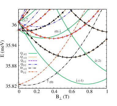
Figure 4: (Color online) The lowest few energy levels with the “m” valley configuration vs. perpendicular magnetic field $B_{\perp}$ in single QDs. Open squares indicate the anticrossing points. The curves with crosslets denote the three-fold degenerate levels (two doublet states and one quartet state) and the ones with solid triangles represent the two-fold degenerate levels (one doublet state and one quartet state). The circle and open triangle at $B_{\perp}=0$ describe the lowest doublet and quartet and doublet. The total orbital angular momentums $L=l_{1}+l_{2}+l_{3}$ are labeled. The half-well width $d=3.926$ nm and the effective diameter $d_{0}=30.3$ nm.

III.2 Vertically coupled double quantum dots

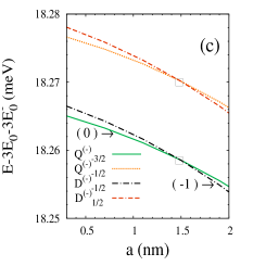
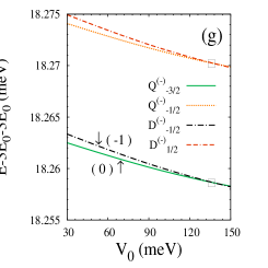
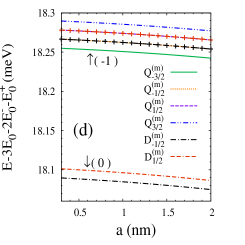
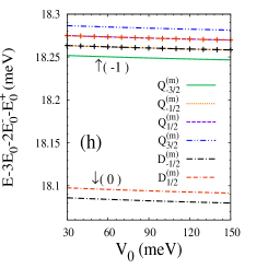
Figure 5: (Color online) (a) and (e) represent the interdot barrier-width and barrier-height dependences of the lowest two subband energies along $z$-direction. (b) and (f) are the valley energies of the lower valley eigenvalue of the lowest two subbands as function of the interdot barrier width and barrier height. (c) and (g) show the three-electron energy spectrum with “$-$” valley configuration, while (d) and (h) give the corresponding spectrum with “m” valley configuration. Open squares in (c) and (g) indicate the anticrossing points. The curves with crosslets denote the three-fold degeneracy of the levels (two doublet states and one quartet state). The total orbital angular momentum $L=l_{1}+l_{2}+l_{3}$ of each states are labeled. Here, the effective diameter $d_{0}=29$ nm, the well width $d=2$ nm and $B_{\perp}=0.1$ T. In (a)-(d), the barrier height $V_{0}=50$ meV. In (e)-(h), the barrier width $a=1$ nm.

In this part, we investigate the vertically coupled DQD case with a perpendicular magnetic field $B_{\perp}=0.1$ T with both the “$-$” and “m” valley configurations. We first study the interdot barrier-width dependence of the “$-$” valley configuration. In Fig. 5(a), the orbital energies of the lowest two subbands along the $z$-direction are plotted as function of interdot barrier width. One can see that the orbital energy of the first subband increases while that of the second subband decreases as the barrier width increases, resulting the decrease of the energy difference $E_{1}-E_{0}$ between them. This corresponds the decrease of the interdot coupling. Differently, the valley energies of the lowest two subbands present oscillation against the barrier width, which can be expected from the formula given in Appendix A. Since the intersubband coupling due to the valley-orbit coupling is much weaker than the intersubband splitting from the orbital degree of freedom, we neglect this term in our calculation. Actually, the first subband dominates the lowest few states because of the large intersubband splitting ($>10$ meV) in the strong interdot coupling regime studied here. The lowest four levels are plotted in Fig. 5(c), where the energies from the subband and valley are subtracted for improving the solution of levels. Similar to the single QD case, the quartet-doublet transition of the ground state can occur and the anticrossing behavior (illustrated as open squares at $a\sim 1.5$ nm) can be observed. We also study the barrier-height dependence with “$-$” valley configuration and plot the results as Fig. 5(e)-(g). In Fig. 5(g), the quartet-doublet transition of the ground state and the anticrossing properties are also present.

As a comparison, we also show the energy spectrum of the “m” valley configuration case as Fig. 5(d) and (h), where the ground state is doublet. In these figures, the curves with crosslets also represent the three-fold degeneracy (two doublet state and one quartet state).

IV SUMMARY

In summary, we have studied three-electron energy spectra in Si/SiGe single QDs and vertically coupled DQDs by using the exact-diagonalization method. In our calculation, the Zeeman splitting, SOC, valley coupling and electron-electron Coulomb interaction are explicitly included. Due to the strong Coulomb interaction, a large number of basis functions are employed to converge the energy spectrum. The ground state energies in single QDs show good agreement with the experiment. As a supplement of the experimental data, we identify the valley configuration, spin configuration and the degeneracy factor of the ground state from our calculation. We then systematically study the ground state configuration in the absence of magnetic field, and find that the ground state is of pure and mixed valley configurations with large and small valley splittings, respectively. We show that the ground state with mixed valley configuration is always doublet. In contrast, the ground state with pure valley configuration is doublet in small dots, while it can be quartet in large dots. Then, we explicitly study the energy spectra of the three-electron states with two typical valley configurations, i.e., pure and mixed valley states, in the presence of perpendicular and parallel magnetic fields. In the pure valley configuration case, we show that the doublet-quartet transition of the ground state can be realized by tuning the magnetic field and/or dot size. For the mixed valley configuration, the doublet-quartet transition of the ground state can also be realized by magnetic field and the three-electron energy spectrum presents interesting quartet-doublet degeneracy, which is connected with the negligible intervalley coupling. Due to the spin-orbit coupling, the intersecting points between the energy levels with identical valley configuration but different spin quantum numbers can present anticrossing behavior, which is expected to benefit the manipulation of spin. We point out and analyze all these anticrossing points in each case. Furthermore, we study the barrier-width and barrier-height dependences of the three-electron energy spectrum in vertically strong-coupled DQDs. We also find anticrossing points in the pure valley configuration case and quartet-doublet degeneracy in the mixed configuration case.

Appendix A VALLEY COUPLING ELEMENTS

$$\Delta^{0}_{0,0} = \frac{V_{\rm v}\hbar^{2}{k_{0}}^{2}{C_{0}}^{2}}{m_{z}}+2V_{\rm v}V_{0}{C_{0}}^{2}\sin^{2}(k_{0}d),$$ (17)

$$\Delta^{1}_{0,0} = \frac{V_{\rm v}\hbar^{2}{k_{0}}^{2}{C_{0}}^{2}\cos[2k_{\rm Si}(\frac{a}{2}+d)]}{m_{z}}$$ (18)

$${}+2V_{\rm v}V_{0}{C_{0}}^{2}\sin^{2}(k_{0}d)\cos(k_{\rm Si}a),$$

$$\Delta^{0}_{1,1} = \frac{V_{\rm v}\hbar^{2}{k_{1}}^{2}{C_{1}}^{2}}{m_{z}}+2V_{\rm v}V_{0}{C_{1}}^{2}\sin^{2}(k_{1}d),$$ (19)

$$\Delta^{1}_{1,1} = \frac{V_{\rm v}\hbar^{2}{k_{1}}^{2}{C_{1}}^{2}\cos(2k_{\rm Si}(\frac{a}{2}+d))}{m_{z}}$$ (20)

$${}+2V_{\rm v}V_{0}{C_{1}}^{2}\sin^{2}(k_{1}d)\cos(k_{\rm Si}a),$$

$$\Delta^{1}_{0,1} = -\Delta^{1}_{1,0}=i\{\frac{V_{\rm v}\hbar^{2}k_{0}k_{1}C_{0}C_{1}}{m_{z}}\sin[k_{\rm Si}(a+2d)]$$ (21)

$${}+2V_{\rm v}V_{0}C_{1}C_{0}\sin(k_{0}d)\sin(k_{1}d)\sin(k_{\rm Si}a)\},$$

where $V_{\rm v}=7.2\times 10^{-11}$ m represents the ratio of the valley coupling strength to the depth of the quantum well potential.Friesen1

Appendix B THREE-ELECTRON BASIS FUNCTIONS

The three-electron basis functions can be constructed in form of either doublet ($S_{\rm tot}=1/2$) or quartet ($S_{\rm tot}=3/2$). We first combine the spin wavefunctions via Clebsch-Gordan coefficients. For the doublet states, the spin functions can be expressed by

$$\chi^{\lambda}_{1/2} = [(\beta_{1}\alpha_{2}+\alpha_{1}\beta_{2})\alpha_{3}-2\alpha_{1}\alpha_{2}\beta_{3}]/{\sqrt{6}}$$

$$\chi^{\lambda}_{-1/2} = [2\beta_{1}\beta_{2}\alpha_{3}-(\beta_{1}\alpha_{2}+\alpha_{1}\beta_{2})\beta_{3}]/{\sqrt{6}}$$

$$\chi^{\rho}_{1/2} = (\beta_{1}\alpha_{2}-\alpha_{1}\beta_{2})\alpha_{3}/{\sqrt{2}}$$

$$\chi^{\rho}_{-1/2} = (\beta_{1}\alpha_{2}-\alpha_{1}\beta_{2})\beta_{3}/{\sqrt{2}},$$ (22)

and for the quartet states, one has

$$\chi^{S}_{3/2} = \alpha_{1}\alpha_{2}\alpha_{3}$$

$$\chi^{S}_{1/2} = (\alpha_{1}\alpha_{2}\beta_{3}+\alpha_{1}\beta_{2}\alpha_{3}+\beta_{1}\alpha_{2}\alpha_{3})/{\sqrt{3}}$$

$$\chi^{S}_{-1/2} = (\alpha_{1}\beta_{2}\beta_{3}+\beta_{1}\beta_{2}\alpha_{3}+\beta_{1}\alpha_{2}\beta_{3})/{\sqrt{3}}$$

$$\chi^{S}_{-3/2} = \beta_{1}\beta_{2}\beta_{3}.$$ (23)

Here, $\alpha_{i}=|\uparrow\rangle_{i}$ and $\beta_{i}=|\downarrow\rangle_{i}$ with the subscript denoting the three electrons. The superscript “S” labels the symmetric configuration for the permutation of any two electrons, while “$\lambda$” and “$\rho$” represent the symmetric and antisymmetric configurations for the permutation only for the electrons “1” and “2”, respectively. With these spin wavefunctions, we then add the corresponding orbital parts to construct the total basis functions. When the three electrons occupy three different orbits, i.e., $N_{i}\neq N_{j}$ with $i,j\in\{1,2,3\}$, one has the total wavefunctions of the doublet states

$$|D^{(\Xi)(1)}_{1/2}\rangle = \phi^{\rho(1)}\chi^{\lambda}_{1/2}-\phi^{\lambda(1)}\chi^{\rho}_{1/2},$$

$$|D^{(\Xi)(2)}_{1/2}\rangle = \phi^{\rho(2)}\chi^{\lambda}_{1/2}-\phi^{\lambda(2)}\chi^{\rho}_{1/2},$$

$$|D^{(\Xi)(1)}_{-1/2}\rangle = \phi^{\rho(1)}\chi^{\lambda}_{-1/2}-\phi^{\lambda(1)}\chi^{\rho}_{-1/2},$$

$$|D^{(\Xi)(2)}_{-1/2}\rangle = \phi^{\rho(2)}\chi^{\lambda}_{-1/2}-\phi^{\lambda(2)}\chi^{\rho}_{-1/2},$$ (24)

and those of the quartet states

$$|Q^{(\Xi)}_{3/2}\rangle = \phi^{A}\chi^{S}_{3/2},$$

$$|Q^{(\Xi)}_{1/2}\rangle = \phi^{A}\chi^{S}_{1/2},$$

$$|Q^{(\Xi)}_{-1/2}\rangle = \phi^{A}\chi^{S}_{-1/2},$$

$$|Q^{(\Xi)}_{-3/2}\rangle = \phi^{A}\chi^{S}_{-3/2}.$$ (25)

When two electrons with opposite spins share the same orbit, i.e., $N_{1}=N_{2}\neq N_{3}$ or $N_{1}\neq N_{2}=N_{3}$ or $N_{1}=N_{3}\neq N_{2}$,

$$|D^{(\Xi)(3)}_{1/2}\rangle = \phi^{\rho}\chi^{\lambda}_{1/2}-\phi^{\lambda}\chi^{\rho}_{1/2},$$

$$|D^{(\Xi)(3)}_{-1/2}\rangle = \phi^{\rho}\chi^{\lambda}_{-1/2}-\phi^{\lambda}\chi^{\rho}_{-1/2}.$$ (26)

Here, {$\phi$} are the corresponding orbital wavefunctions. The superscript “A” on the right hand side of Eq. (25) describes the permutation antisymmetric character for the exchange of any two electrons and the “$(1)$” and “$(2)$” in the superscripts of Eq. (24) are used to distinguish the two doublet configurations with the same spin magnetic quantum numbers or the two orbital functions with the same symmetry. The orbital wavefunctions can be expressed as

$$\left\{\begin{array}[]{llllll}\phi^{A}&=&\tfrac{1}{\sqrt{6}}(|N_{1}N_{2}N_{3}\rangle-|N_{1}N_{3}N_{2}\rangle+|N_{2}N_{3}N_{1}\rangle-|N_{2}N_{1}N_{3}\rangle+|N_{3}N_{1}N_{2}\rangle-|N_{3}N_{2}N_{1}\rangle)\\[2.0pt] \phi^{\rho(1)}&=&\tfrac{1}{2\sqrt{2}}(|N_{3}N_{2}N_{1}\rangle-|N_{2}N_{3}N_{1}\rangle+|N_{3}N_{1}N_{2}\rangle-|N_{1}N_{3}N_{2}\rangle)\\[2.0pt] \phi^{\lambda(1)}&=&\tfrac{1}{2\sqrt{6}}(|N_{1}N_{3}N_{2}\rangle+|N_{2}N_{3}N_{1}\rangle+|N_{3}N_{2}N_{1}\rangle+|N_{3}N_{1}N_{2}\rangle-2|N_{1}N_{2}N_{3}\rangle-2|N_{2}N_{1}N_{3}\rangle)\\[2.0pt] \phi^{\rho(2)}&=&\tfrac{1}{2\sqrt{6}}(2|N_{1}N_{2}N_{3}\rangle-2|N_{2}N_{1}N_{3}\rangle-|N_{2}N_{3}N_{1}\rangle+|N_{3}N_{2}N_{1}\rangle-|N_{3}N_{1}N_{2}\rangle+|N_{1}N_{3}N_{2}\rangle)\\[2.0pt] \phi^{\lambda(2)}&=&\tfrac{1}{2\sqrt{2}}(|N_{3}N_{1}N_{2}\rangle-|N_{3}N_{2}N_{1}\rangle+|N_{1}N_{3}N_{2}\rangle-|N_{2}N_{3}N_{1}\rangle),\end{array}\right.$$ (32)

$$\phi^{\rho}=\left\{\begin{array}[]{llllll}\tfrac{1}{2}(|N_{1}N_{3}N_{1}\rangle-|N_{3}N_{1}N_{1}\rangle),&&N_{1}=N_{2}\neq N_{3},\\[2.0pt] \tfrac{1}{2}(|N_{1}N_{2}N_{2}\rangle-|N_{2}N_{1}N_{2}\rangle),&&N_{1}\neq N_{2}=N_{3},\\[2.0pt] \tfrac{1}{2}(|N_{1}N_{2}N_{1}\rangle-|N_{2}N_{1}N_{1}\rangle),&&N_{1}=N_{3}\neq N_{2},\end{array}\right.$$ (36)

$$\phi^{\lambda}=\left\{\begin{array}[]{llllll}\tfrac{1}{2\sqrt{3}}(2|N_{1}N_{1}N_{3}\rangle-|N_{1}N_{3}N_{1}\rangle-|N_{3}N_{1}N_{1}\rangle),N_{1}=N_{2}\neq N_{3},\\[2.0pt] \tfrac{1}{2\sqrt{3}}(|N_{2}N_{1}N_{2}\rangle+|N_{1}N_{2}N_{2}\rangle-2|N_{2}N_{2}N_{1}\rangle),N_{1}\neq N_{2}=N_{3},\\[4.0pt] \tfrac{1}{2\sqrt{3}}(2|N_{1}N_{1}N_{2}\rangle-|N_{1}N_{2}N_{1}\rangle-|N_{2}N_{1}N_{1}\rangle),N_{1}=N_{3}\neq N_{2}.\end{array}\right.$$ (40)

Appendix C MATRIX ELEMENTS OF COULOMB INTERACTION

The Coulomb interaction components readShen1 ; Lwang1 ; Lwang2

$$\langle N_{1}N_{2}N_{3}|H^{ij}_{\rm C}|N_{1}^{\prime}N_{2}^{\prime}N_{3}^{\prime}\rangle=\frac{e^{2}}{16\pi^{2}\varepsilon_{0}\kappa}\delta_{N_{k},N_{k}^{\prime}}\delta_{l_{i}+l_{j},l_{i}^{\prime}+l_{j}^{\prime}}\sum_{\gamma_{i},\gamma_{j},\gamma^{\prime}_{i},\gamma^{\prime}_{j}=z,\overline{z}}\eta^{\gamma_{i}}_{n_{{\rm v}i}}\eta^{\gamma_{j}}_{n_{{\rm v}j}}\eta^{\gamma^{\prime}_{i}}_{n^{\prime}_{{\rm v}i}}\eta^{\gamma^{\prime}_{j}}_{n^{\prime}_{{\rm v}j}}U(\phi^{\gamma_{i}}_{n_{i}l_{i}n_{zi}},\phi^{\gamma_{j}}_{n_{j}l_{j}n_{zj}},\phi^{\gamma^{\prime}_{i}}_{n^{\prime}_{i}l^{\prime}_{i}n^{\prime}_{zi}},\phi^{\gamma^{\prime}_{j}}_{n^{\prime}_{j}l^{\prime}_{j}n^{\prime}_{zj}})$$ (41)

with $\{i,j,k\}=\{1,2,3\}$. Here, $|N_{i}\rangle\equiv|n_{i}l_{i}n_{zi}n_{{\rm v}i}\rangle$ is the single-electron wavefunction of the $i$-th electron. Superscripts $\gamma_{i(j)}$ and $\gamma^{\prime}_{i(j)}$ run over the two valleys with $\eta^{z}_{\pm}=1$ and $\eta^{\overline{z}}_{+}=-\eta^{\overline{z}}_{-}=1$ (Ref. Lwang1, ). $U$ in Eq. (41) can be expressed asLwang1 ; Shen1

$$U(\phi^{\gamma_{1}}_{n_{1}l_{1}n_{z1}},\phi^{\gamma_{2}}_{n_{2}l_{2}n_{z2}},\phi^{\gamma^{\prime}_{1}}_{n^{\prime}_{1}l^{\prime}_{1}n^{\prime}_{z1}},\phi^{\gamma^{\prime}_{2}}_{n^{\prime}_{2}l^{\prime}_{2}n^{\prime}_{z2}})=\int^{\infty}_{0}\mathrm{d}k_{\parallel}\int^{\infty}_{-\infty}\mathrm{d}k_{z}k_{\parallel}P^{n^{\prime}_{1}l^{\prime}_{1}}_{n_{1}l_{1}}(k_{\parallel})P^{n_{2}l_{2}}_{n^{\prime}_{2}l^{\prime}_{2}}(k_{\parallel})\frac{W^{n^{\prime}_{z_{1}}\gamma^{\prime}_{1}}_{n_{z_{1}}\gamma_{1}}(k_{z})[W^{n_{z_{2}}\gamma_{2}}_{n^{\prime}_{z_{2}}\gamma^{\prime}_{2}}(k_{z})]^{*}}{k^{2}}.$$

(42)

$P^{n^{\prime}l^{\prime}}_{nl}$ can be obtained from the lateral part of the integral $\langle nln_{z}\gamma|e^{i{\mathbf{k}}\cdot{\mathbf{r}}}|n^{\prime}l^{\prime}n^{\prime}_{z}\gamma^{\prime}\rangle$.

$$P^{n^{\prime}l^{\prime}}_{nl} = \sqrt{\frac{n!n^{\prime}!}{(n+|l|)!(n^{\prime}+|l^{\prime}|)!}}e^{-\frac{k^{2}_{\parallel}}{4\alpha^{2}}}\sum_{i=0}^{n^{\prime}}\sum_{j=0}^{n}C^{i}_{n^{\prime},|l^{\prime}|}C^{j}_{n,|l|}\overline{n}!L^{|l-l^{\prime}|}_{\overline{n}}(\frac{k^{2}_{\parallel}}{4\alpha^{2}})[{\rm sgn}(l^{\prime}-l)\frac{k_{\parallel}}{2\alpha}]^{|l^{\prime}-l|},$$ (43)

with $C^{i}_{n,l}=\frac{(-1)^{i}}{i!}\binom{n+l}{n-i}$, $\overline{n}=i+j+\frac{|l|+|l^{\prime}|-|l-l^{\prime}|}{2}$ and ${\rm sgn}(x)$ being the sign function. $W^{n^{\prime}_{z}\gamma^{\prime}}_{n_{z}\gamma}$ in Eq. (42) is the integral $\langle n_{z}\gamma|{\rm exp}(ik_{z}z)|n^{\prime}_{z}\gamma^{\prime}\rangle$.

References

• (1) D. Loss and D. P. DiVincenzo, Phys. Rev. A 57, 120 (1998).
• (2) S. M. Reimann and M. Maminen, Rev. Mod. Phys. 74, 1283 (2002).
• (3) R. Hanson, L. P. Kouwenhoven, J. R. Petta, S. Tarucha, and L. M. K. Vandersypen, Rev. Mod. Phys. 79, 1217 (2007).
• (4) M. W. Wu, J. H. Jiang, and M. Q. Weng, Phys. Rep. 493, 61 (2010).
• (5) J. Berezovsky, M. H. Mikkelsem, N. G. Stoltz, L. A. Coldren, and D. D. Awschalom, Science 320, 349 (2008).
• (6) M. A. Eriksson, M. Friesen, S. N. Coppersmith, R. Joynt, L. J. Klein, K. Slinker, C. Tahan, P. M. Mooney, J. O. Chu, and S. J. Koester, Quantum Inf. Process. 3, 133 (2004).
• (7) D. Culcer, L. Cywi$\acute{\rm n}$ski, Q. Li, X. Hu, and S. Das Sarma, Phys. Rev. B 80, 205302 (2009).
• (8) L. Wang, K. Shen, B. Y. Sun, and M. W. Wu, Phys. Rev. B 81, 235326 (2010).
• (9) D. Culcer, L. Cywi$\acute{\rm n}$ski, Q. Li, X. Hu, and S. Das Sarma, Phys. Rev. B 82, 155312 (2010).
• (10) L. Wang and M. W. Wu, J. Appl. Phys. 110, 043716 (2011).
• (11) D. Culcer, A. L. Saraiva, B. Koiller, X. Hu, and S. Das Sarma, arXiv:1107.0003v1.
• (12) J. S$\ddot{\rm a}$rkk$\ddot{\rm a}$ and A. Harju, New J. Phys. 13, 043010 (2011).
• (13) C. Tahan, M. Friesen, and R. Joynt, Phys. Rev. B 66, 035314 (2002).
• (14) A. R. Calderbank and P. W. Shor, Phys. Rev. A 54, 1098 (1996).
• (15) M. S. Sherwin, A. Imamoglu, and T. Montroy, Phys. Rev. A 60, 3508 (1999).
• (16) C. H. Bennett, D. P. DiVincenzo, J. A. Smolin, and W. K. Wootters, Phys. Rev. A 54, 2636 (1996).
• (17) D. G. Cory, M. D. Price, W. Maas, E. Knill, R. Laflamme, W. H. Zurek, T. F. Havel, and S. S. Somaroo, Phys. Rev. Lett. 81, 2152 (1998).
• (18) G. Dresselhaus, Phys. Rev. 100, 580 (1955).
• (19) E. I. Rashba, Fiz. Tiverd. Tela (Leningrad) 2, 1224 (1960).
• (20) L. Vervoort, R. Ferreira, and P. Voisin, Phys. Rev. B 56, R12744 (1997).
• (21) L. Vervoort, R. Ferreira, and P. Voisin, Semicond. Sci. Technol. 14, 227 (1999).
• (22) M. O. Nestoklon, E. L. Ivchenko, J.-M. Jancu, and P. Voisin, Phys. Rev. B 77, 155328 (2008).
• (23) Semiconductors, Landolt-Börnstein, New Series, Vol. 17, Pt. A, edited by O. Madelung (Springer-Verlag, Berlin, 1987).
• (24) U. Bockelmann and G. Bastard, Phys. Rev. B 42, 8947 (1990).
• (25) Q. Li, L. Cywi$\acute{\rm n}$ski, D. Culcer, X. Hu, and S. Das Sarma, Phys. Rev. B 81, 085313 (2010).
• (26) M. Friesen, S. Chutia, C. Tahan, and S. N. Coppersmith, Phys. Rev. B 75, 115318 (2007).
• (27) T. Ando, A. B. Fowler, and F. Stern, Rev. Mod. Phys. 54, 437 (1982).
• (28) W. H. Lim, F. A. Zwanenburg, H. Huebl, M. M$\ddot{\rm o}$tt$\ddot{\rm o}$nen, K. W. Chan, A. Morello, and A. S. Dzurak, Appl. Phys. Lett. 95, 242102 (2009).
• (29) M. Xiao, M. G. House, and H. W. Jiang, Appl. Phys. Lett. 97, 032103 (2010).
• (30) W. H. Lim, C. H. Yang, F. A. Zwanenburg, and A. S. Dzurak, Nanotechnology 22, 335704 (2011).
• (31) M. G. Borselli, R. S. Ross, A. A. Kiselev, E. T. Croke, K. S. Holabird, P. W. Deelman, L. D. Warren, I. Alvarado-Rodriguez, I. Milosavljevic, F. C. Ku, W. S. Wong, A. E. Schmitz, M. Sokolich, M. F. Gyure, and A. T. Hunter, Appl. Phys. Lett. 98, 123118 (2011).
• (32) M. Raith, P. Stano, and J. Fabian, Phys. Rev. B 83, 195318 (2011).
• (33) E. Barnes, J. P. Kestner, N. T. T. Nguyen, and S. Das Sarma, arXiv:1108.1399v1.
• (34) S. Tarucha, T. Honda, D. G. Austing, Y. Tokura, K. Muraki, T. H. Oosterkamp, J. W. Janssen, L. P. Kouwenhoven, Physica E 3, 112 (1998).
• (35) G. P. Garcia, V. Pellegrini, A. Pinczuk, M. Rontani, G. Goldoni, E. Molinari, B. S. Dennis, L. N. Pfeiffer, and K. W. West, Phys. Rev. Lett. 95, 266806 (2005).
• (36) J. I. Climente, A. Bertoni, M. Rontani, G. Goldoni, and E. Molinari, Phys. Rev. B 74, 125303 (2006).
• (37) J. I. Climente, A. Bertoni, G. Goldoni, M. Rontani, and E. Molinari, Phys. Rev. B 76, 085305 (2007).
• (38) A. Gamucci, V. Pellegrini, A. Singha, A. Pinczuk, L. N. Pfeiffer, K. W. West, and M. Rontani, arXiv:1109.4758v1.
• (39) Y. Hada and M. Eto, Phys. Rev. B 68, 155322 (2003).
• (40) M. Eto, Jpn. J. Appl. Phys. 40, 1929 (2001).
• (41) Y. Y. Wang and M. W. Wu, Phys. Rev. B 74, 165312 (2006); ibid. 77, 125323 (2008).
• (42) K. Shen and M. W. Wu, Phys. Rev. B 76, 235313 (2007).
• (43) V. Fock, Z. Phys. 47, 446 (1928).
• (44) C. G. Darwin, Proc. Cambridge Philos. Soc. 27, 86 (1931).
• (45) J. L. Cheng, M. W. Wu, and C. L$\ddot{\rm u}$, Phys. Rev. B 69, 115318 (2004).
• (46) R. N. Dexter, B. Lax, A. F. Kip, and G. Dresselhaus, Phys. Rev. 96, 222 (1954).
• (47) C. F. O. Graeff, M. S. Brandt, M. Stutzmann, M. Holzmann, G. Abstreiter, and F. Sch$\ddot{\rm a}$ffler, Phys. Rev. B 59, 13242 (1999).
• (48) We calculate ground state energies of one, two and three electrons to obtain $\Delta\mu_{i}$ ($N_{i}=1,2$) via our model with $d_{0}$ being a fitting parameter. We choose $d_{0}$ which minimizes $\sqrt{(\Delta\mu_{1}-\Delta\mu^{*}_{1})^{2}+(\Delta\mu_{2}-\Delta\mu^{*}_{2})^{2}}$ with $\Delta\mu^{*}_{i}$ representing the experimental value.
• (49) In fact, from the fitting of the valley splitting, one can obtain many solutions of the well width because of the oscillation of the valley splitting against well width. However, the variation of the well width only induce slight effect on the addition energies, e.g., within $\sim 0.1$ % modification when the well width of Si4 varies $2$ nm. In our calculation, we choose one of these solutions near the suggested half-well width ($\sim 4$ nm). For the same reason, we use the same well width in Si1 and Si2 as that in Si3 as a reasonable approximation.
• (50) J. R. Petta, A. C. Johnson, J. M. Taylor, E. A. Laird, A. Yacoby, M. D. Lukin, C. M. Marcus, M. P. Hanson, and A. C. Gossard, Science 309, 2180 (2005).
• (51) K. C. Nowack, F. H. Koppens, Y. V. Nazarov, and L. M. K. Vandersypen, Science 318, 1430 (2007).
• (52) J. S$\ddot{\rm a}$rkk$\ddot{\rm a}$ and A. Harju, Phys. Rev. B 80, 045323 (2009).
• (53) E. A. Laird, J. M. Taylor, D. P. DiVincenzo, C. M. Marcus, M. P. Hanson, and A. C. Gossard, Phys. Rev. B 82, 075403 (2010).
• (54) J. R. Petta, H. Lu, and A. C. Gossard, Science 327, 669 (2010).
• (55) From the explicit expression of the three-electron Hamiltonian, one can demonstrate that the Hamiltonian without spin-orbit term is non-vanishing only between states with the same total orbital angular momentum $L=l_{1}+l_{2}+l_{3}$. And the spin-orbit coupling is very weak compared with the orbital energy and Coulomb interaction. Therefore, one can denote each state (except in the vicinity of the anticrossing points) by the total orbital angular momentum.
• (56) Here we take $n_{v1}=n_{v2}=-$ and $n_{v3}=+$ for the permutation antisymmetric or symmetric characters of the orbital part of the basis functions for the electrons “1” and “2”. Even though, the identity among the three electrons is still guaranteed by the orthogonality and completeness of the entire Hilbert space.