An analysis of a regular black hole interior model

Abstract

We analyze the thermodynamical properties of the regular static and spherically symmetric black hole interior model presented by Mboyne and Kazanas. Equations for the thermodynamical quantities valid for an arbitrary density profile are deduced, and from them we show that the model is thermodynamically unstable. Evidence is also presented pointing to its dynamical instability. The gravitational entropy of this solution based on the Weyl curvature conjecture is calculated, following the recipe given by Rudjord, Gr$\varnothing$n and Sigbj$\varnothing$rn, and it is shown to have the expected behavior.

1 Introduction

The existence of singularities in some solutions of General Relativity is one of the most important unresolved issues in the classical description of the gravitational field. Singularities are an undesirable feature of any theory of gravitation: they can be naturally considered as a source of lawlessness (see for instance earman ), because the space-time description breaks down “there”, and physical laws presuppose space-time. There are several ways in which singularities can be avoided (see physrep for the case of Cosmology), both at the classical and at the quantum level. Since there is no widely-accepted theory of quantum gravity, the issue of singularities in General Relativity has been addressed from classical considerations in various fashions. One particular approach is the introduction of a limiting curvature hypothesis, based on that, at a singularity, invariants constructed with the Riemann tensor generally diverge. Hence, a suitable way to eliminate singularities would be to impose a limiting principle on the curvature, associated with a fundamental scale (it may be the Planck scale). This hypothesis (first proposed in markov ) is implemented by demanding that any solution of the field equations must reduce to a definite nonsingular solution (for instance to a de Sitter space-time) when some of the invariants attain their limiting values, in such a way that the strong energy condition (one of the hypothesis of the singularity theorems s1 s2 s3 ) is violated.

A theory based on this hypothesis has been implemented by modifying the dynamics of General Relativity with the addition of nonlinear terms in Ref. bran . However, there is another approach, suggested by Gliner gli , that consists of assuming that the micro-physics of high-density matter is such that a phase transition must occur leading any system under such extreme conditions to the de Sitter geometry. Models of this type were also considered by Sakharov sak , Zeldovich zel , and Bardeen baar . In these models the space-time metric behaves as the Schwarzschild metric for large radii and, as de Sitter’s towards the core of the object. Regular black hole models with direct matching of the de Sitter interior and the Schwarzschild exterior have been proposed by Poisson and Israel poi , Frolov et al. frolov89 ; frolov90 , and Dymnikova dy2003 .

An exact solution of the Einstein field equations containing at the core a de Sitter fluid was found by Dymnikova dy . This solution represents a vacuum nonsingular black hole. The stress-energy tensor which is the source of curvature “describes a smooth transition from the standard vacuum state at infinity to (an) isotropic vacuum state at $r\rightarrow 0$ through (an) anisotropic vacuum state in (the) intermediate region […]. At the present such a transitional material cannot be described starting from any fundamental theory describing reality at the microscopic level”.

This anisotropic vacuum state was replaced by Mbonye and Kazanas (MK) mk with a region filled with matter under both radial and tangential pressures, described by an equation of state (EOS) that relates the radial pressure to the density and smoothly reproduces the de Sitter’s spacetime behavior near $r=0$, tending to a polytrope at larger $r$, low $\rho$ values.

The main goal of the present work is to study the MK model for a regular black hole in which the singularity is avoided precisely by the second method mentioned above. In particular, a detailed study of the thermodynamical aspects of the matter that is the source of the curvature and of the gravitational field will be given. It will be shown that the solution is thermodynamically unstable, and we shall present evidence supporting the dynamical instability of the model. The issue of the gravitational entropy of this model will be also addressed, following the ideas presented in Gron (see also Romero et al. us ).

We shall begin in Sect.2 with a short review of the regular black hole solution advanced in mk . Its thermodynamical properties will be discussed in Sect.3, and the stability will be analyzed in Sect.4. In Sect.5, the gravitational entropy of the MK solution will be calculated. These results will be analyzed in Sect.6.

2 A model of a regular black hole interior

The model introduced in mk represents a regular static black hole, with a matter source that smoothly goes from a de Sitter behavior near the origin to Schwarzschild’s space-time outside the object. A space-time metric well-adapted to examine the properties of this system is mk2 :

$$ds^{2}=-B(r)dt^{2}+\left(1-\frac{2m(r)}{r}\right)^{-1}dr^{2}+r^{2}(d\theta^{2}+\sin^{2}\theta d\phi^{2}).$$ (1)

The EOS proposed by Mbonye and Kazanas mk is given by:

$$p_{r}(\rho)=\left[\alpha-(\alpha+1)\left(\frac{\rho}{\rho_{\textsf{max}}}\right)^{2}\right]\left(\frac{\rho}{\rho_{\textsf{max}}}\right)\rho,$$ (2)

where $p_{r}$ is the radial pressure (to be distinguished from the tangential pressure, which is needed in these models to satisfy the Tolman-Oppenheimer-Volkoff (TOV) equation), and $\alpha=2.2135$ . Such an equation describes the behavior of matter that changes smoothly from normal to a core of “exotic fluid” with an EOS that approaches $p_{r}=-\rho$ when $r\rightarrow 0$ (see Figure 1). It follows that in order to avoid the presence of the singularity at $r=0$, the strong energy condition is violated in the core of the object, whereas the weak energy condition and dominant energy condition are everywhere satisfied mk .

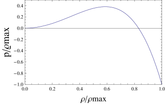
Figure 1: Plot of (1), that gives the relation between the radial pressure and the density.

MK chose the density profile suggested by Dymnikova to solve Einstein’s equations at small $r$dy :

$$\rho(r)=\rho_{\textsf{max}}e^{-8\frac{r^{3}}{R^{3}}},$$ (3)

where $R^{3}=8R_{\rm S}r_{0}^{2}$, $R_{\rm S}$ is the Schwarzschild radius,

$$r_{0}=\left(\frac{3}{8\pi\rho_{\textsf{max}}}\right)^{1/2},$$ (4)

and $\rho_{\rm max}$ is of the order of the Planck density. It follows from (3) that (almost) all the mass is contained inside a sphere of radius $R$ well within the black hole, which corresponds to the surface of the object inside the horizon. The density undergoes a smooth transition from the de Sitter state at the center to the vacuum state for $r>R$, with an intermediate region of non-inflationary material, a situation that was anticipated in poi .

From Eq. 1, when $r\rightarrow\infty$, $m(r)\rightarrow M$, and the external metric ($r>>R_{\rm S}$ becomes asymptotically Schwarzschild.

The structure of the black hole interior is characterized by the followings regions, as described in mk :

1. Exotic matter region:

   $$0\leq r\leq r_{*}=0.4R,$$ (5)

   where $R$ is the radius of the compact object inside the horizon. At the core of this region the metric is de Sitter.
   

2. Normal matter region:

   $$0.4R\leq r\leq R.$$ (6)

   This region is supported against collapse by the de Sitter core.
   

3. Schwarzschild vacuum region:

   $$R<r<r_{{\rm h}}=2M,$$ (7)

   where $r_{{\rm h}}=R_{\rm S}=2M$ is the radius of the event horizon. In this region the Ricci tensor is null.

We emphasize that the space-time metric is exactly de Sitter at the geometrical center of the object and, for $r>R$ it quickly tends to Schwarzschild.

The plot of the radial pressure as a function of the radial coordinate is shown in Figure 2. It can be seen that the pressure follows the equation $p=-\rho$ at the core of the object, and it goes to zero at $r/R=1$, the surface of the matter region. The radial pressure has another zero located at $r/R=0.28$, two inflexion points at $r/R=0.26$ and $r/R=0.5$, and an absolute maximum at $r/R=0.4$. The exotic matter (for which the pressure decreases with decreasing $r$) occupies the region $r/R<0.4$ .

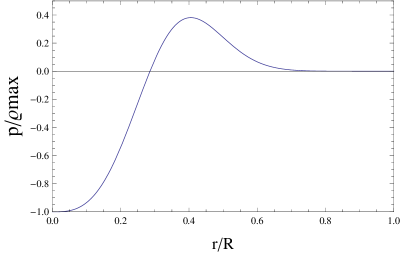
Figure 2: Radial pressure as a function of the radial coordinate inside the regular black hole considered in the text.

The solution of the Einstein field equations $G^{\mu}_{\nu}=-8\pi T^{\mu}_{\nu}$, with:

$$T^{\mu}_{\nu}={\rm diag}(\rho(r),p_{r}(r),p_{\perp}(r),p_{\perp}(r)),$$

for the metric given in (1) and the EOS (2) takes the form mk2 :

$$B(r) = \exp\int^{r}_{r_{0}}\frac{2}{r^{\prime 2}}\left[m(r^{\prime})+4\pi r^{\prime 3}p_{r^{\prime}}\right]$$ (8)

$$\times\left[\frac{1}{\left(1-\frac{2m(r^{\prime})}{r^{\prime}}\right)}\right]dr^{\prime}.$$

The total mass of the object is given by:

$$M=\int^{R}_{0}m(r)dr,$$ (9)

where:

$$m(r)=4\pi\int^{r}_{0}\rho(r^{\prime})r^{\prime 2}dr^{\prime}.$$ (10)

Equations (8) and (10) describe the geometry of the space-time of the regular black hole introduced in mk . Since the EOS and the density as a function of $r$ were specified in mk , the tangential pressure in terms of the given quantities follows from the Einstein field equations. Explicitly:

$$p_{\bot}=p_{r}+\frac{r}{2}p^{\prime}_{r}+\frac{1}{2}\left(p_{r}+\rho\right)\left[\frac{m(r)+4\pi r^{3}p_{r}}{r-2m(r)}\right].$$ (11)

The behavior of the tangential pressure with $r$ is given in Figure 3.

Figure 3: Plot of the tangential pressure as a function of the radial coordinate, given by (11).

It is important to emphasize at this point that the MK model differs from the usual approach (see for instance horvat ), in the sense that, whereas in the former one the EOS and the explicit form of $\rho(r)$ were given, in the latter two relations between the quantities $p_{r}$, $p_{\perp}$ and $\rho$ are advanced. As shown in the Appendix, the choice in the MK model has important consequences in the analysis of the perturbations of the field equations.

3 Thermodynamics of the matter inside the horizon

Following mk , we shall start by assuming that the body has reached a static equilibrium configuration (i.e inside the black hole, the pull of the gravitational field is balanced by the repulsion exerted by the exotic matter). It will also be assumed that matter is in thermodynamic equilibrium. As shown below, the results obtained under these hypotheses turn out to be incorrect, and hence they imply that the system is both dynamically and thermodynamically unstable.

The temperature of the matter as a function of the radius can be estimated from the laws of standard thermodynamics:

$$TdS=d(\rho V)+p_{\textbf{{r}}}dV,$$ (12)

where $dV$ is an element of volume in the proper reference frame of the fluid gravitation . From here, using $\partial^{2}S/\partial V\partial T=\partial^{2}S/\partial T\partial V$:

$$dp_{r}=\frac{\left(\rho+p_{r}\right)}{T}dT.$$ (13)

If we replace (2) and (3) into (13) we get:

$$\frac{dT}{T}=\frac{2\left[\alpha-2(\alpha+1)(\rho/\rho_{\textsf{max}})^{2}\right]d\rho}{\rho_{\textsf{max}}+\left[\alpha-(\alpha+1)(\rho/\rho_{\textsf{max}})^{2}\right]\rho}.$$ (14)

We obtain the formula of the temperature as a function of the radial coordinate by integration of (14):

$$\frac{T}{T_{\textsf{sup}}}=\left[1+\alpha e^{-8r^{3}/R^{3}}-(\alpha+1)e^{-24r^{3}/R^{3}}\right]^{4/3}e^{\Xi(r)},$$ (15)

where $T_{\rm{sup}}$ stands for the temperature of the the matter field at $r=R$, and:

$$\Xi(r)=\frac{2}{3}\int^{e^{-8r^{3}/R^{3}}}_{0}\frac{\alpha d(\rho/\rho_{\textsf{max}})}{1+\alpha(\rho/\rho_{\textsf{max}})-(\alpha+1)(\rho/\rho_{\textsf{max}})^{3}}.$$ (16)

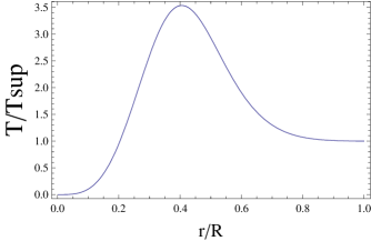
Figure 4: Temperature as a function of the radial coordinate inside the black hole, given by (15). $T_{\rm{sup}}$ stands for the temperature of the the matter field at $r=R$.

Figure 4 displays the temperature of the matter as a function of the radius. We note that the temperature tends to absolute zero close to the core. As for the pressure, there is only one maximum at $r/R=0.4$. The inflexion points of $T(r)$ occur at $r/R=0.31$ and at $r/R=0.57$.

An expression for the entropy (up to an additive constant) as a function of the coordinates can be obtained by substituting (15) in (12):

$$S\equiv\frac{(\rho+p)}{T}V.$$ (17)

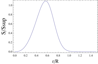
Figure 5: Entropy of the matter field as a function of the radial coordinate inside the black hole. $S_{\rm{sup}}$ stands for the entropy of the the matter field at $r=R$.

The result is plotted in Figure 5. The entropy goes to zero as $r\rightarrow 0$ in accordance to Nerst’s theorem, and it has a maximum close to $r/R=0.4$, in the region of highest density of normal matter.

The entropy density of the matter inside the regular black hole can also be calculated, and is given by:

$$\frac{s}{s_{\textsf{R/2}}}=\frac{(\rho/\rho_{\textsf{max}})[1+\alpha(\rho/\rho_{\textsf{max}})-(\alpha+1)(\rho/\rho_{\textsf{max}})^{3}]^{-1/3}}{0.2076e^{(2/3)\int^{\rho}_{0}\alpha d\rho[\rho_{\textsf{max}}+\alpha\rho-(\alpha+1)(\rho^{3}/\rho_{\textsf{max}}^{2})]^{-1}}}.$$ (18)

The plots of the entropy density as a function of $\rho$ and $r$ are shown in Figures 6 and 7. It can be seen that the entropy density diverges at the origin as a consequence of the vanishing volume. The entropy density as a function of the density has one inflexion point at $\rho/\rho_{\small{\rm{max}}}=0.73$ which is located at $r/R=0.34$.

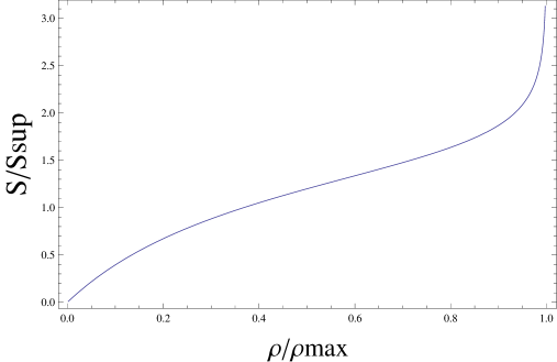
Figure 6: Entropy density of the matter inside the black hole as a function of the density. $S_{\rm{sup}}$ stands for the entropy of the matter field at $r=R$.

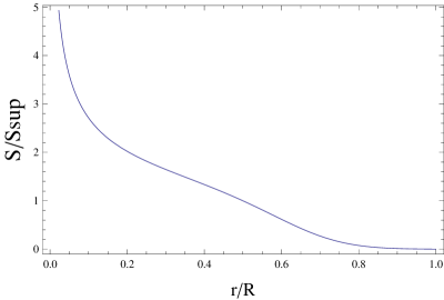
Figure 7: Entropy density of the matter inside the black hole as a function of the radial coordinate. $S_{\rm{sup}}$ stands for the entropy of the matter field at $r=R$.

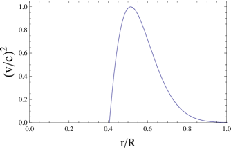
Figure 8: Sound speed as a function of the radial coordinate.

The radial sound speed as a function of the energy density follows from $\ v_{r}^{2}=dp/d\rho$ (with $c=1$), yielding:

$$v_{r}^{2}=2e^{-8r^{3}/R^{3}}\left[\alpha-2(\alpha+1)e^{-16r^{3}/R^{3}}\right].$$ (19)

The result is shown in Figure 8. From Figures 2 and 8, we see that the sound speed is zero at the value of $r/R$ for which the pressure is maximum. In addition, the sound speed takes complex values in the region $r/R<0.4$, in accordance with the negative slope of the equation of state as a function of the density (see (2) and Figure 1). The fact that sound waves do not propagate in the region $r/R<0.4$ is a consequence of the exotic behavior of the fluid there: a variation in pressure causes an expansion rather than a compression.

To discuss the thermodynamical equilibrium we shall need below the Helmholtz free energy, given by $F=U-TS=-pV$. Explicitly:

$$\frac{F}{F_{0.2R}}=\frac{-1}{0.018}\left[\alpha-(\alpha+1)\left(\frac{\rho}{\rho_{\text{max}}}\right)^{2}\right]\left(\frac{\rho}{\rho_{\text{max}}}\right)^{2}\frac{4\pi}{3}\left(\frac{r}{R}\right)^{3}.$$ (20)

The plot of the Helmholtz free energy $F$ as a function of the radial coordinate is shown in Figure 9.

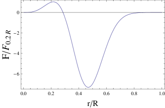
Figure 9: Helmholtz free energy as a function of the radial coordinate. $F_{0.2R}$ stands for the Helmholtz free energy at $r/R=0.2$.

Using the functions discussed in this section, we shall discuss in the next one the issue of thermodynamical and dynamical equilibrium.

4 Equilibrium of the black hole interior configuration

4.1 Thermodynamical equilibrium

A condition for a system to be in stable thermodynamical equilibrium is that, for a given value of entropy and volume, the energy must be minimum. This is equivalent to impose on the the specific heat at constant volume the condition:

$$C_{V}>0.$$ (21)

The dependence of $C_{V}$ with the radial coordinate can be calculated from:

$$C_{V}=T\left(\frac{dS}{dT}\right)_{V}.$$ (22)

Using the expressions deduced in the previous sections, we obtain:

$$\frac{C_{\text{V}}}{V} = \frac{1}{2T}\frac{\rho_{\text{max}}\left(1+\left[\alpha-(\alpha+1)\left(\frac{\rho}{\rho_{\text{max}}}\right)^{2}\right]\frac{\rho}{\rho_{\text{max}}}\right)}{\left[\alpha-2(\alpha+1)\left(\frac{\rho}{\rho_{\text{max}}}\right)^{2}\right]}.$$ (23)

For $r=R$, $\rho$ is zero, and (23) yields:

$$\frac{C_{\text{Vsup}}}{V_{\text{sup}}}=\frac{\rho_{\text{max}}}{2\alpha T_{\text{sup}}}.$$ (24)

Introducing this expression as a constant of normalization in (23), it follows that:

$$\frac{C_{\text{V}}}{C_{\text{Vsup}}}=\left(\frac{r}{R}\right)^{3}\frac{\alpha\left(1+\left[\alpha-(\alpha+1)\left(\frac{\rho}{\rho_{\text{max}}}\right)^{2}\right]\frac{\rho}{\rho_{\text{max}}}\right)}{\left[\alpha-2(\alpha+1)\left(\frac{\rho}{\rho_{\text{max}}}\right)^{2}\right]}\frac{T_{\text{sup}}}{T}.$$ (25)

The plot of the specific heat at constant volume is shown in Figure 10. We can see that the specific heat is negative for $r/R<0.4$ and positive for $r/R>0.4$. For $r/R=0.4$ it is not defined. The change of sign in $C_{{\rm V}}$ can be understood from Figures 4 and 6, taking into account that (22) can also be written as:

$$C_{V}=T\left(\frac{dS}{d\rho}\right)_{V}\left(\frac{d\rho}{dT}\right)_{V}.$$ (26)

Since the slope of the entropy as a function of the density is always positive, the change of sign is determined by $d\rho/dT$, which can also be written as $d\rho/dT=(d\rho/dr)\;(dr/dT)$. The density as a function of $r$ is a decreasing exponential function so, $d\rho/dr<0$ for any value of the radius. From Figure 4 we see that for $r/R<0.4$, $dr/dT>0$ and $d\rho/dT$ becomes negative in that region; instead for $r/R>0.4$, $dr/dT<0$ and $d\rho/dT>0$ in the normal matter region.

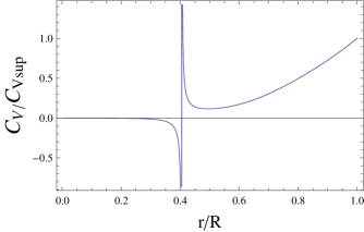
Figure 10: Specific heat at constant volume as a function of the radial coordinate in the black hole interior. $C_{V{\rm sup}}$ stands for the specific heat at constant volume at $r=R$.

Similarly, we can calculate the specific heat at constant pressure, defined by:

$$C_{\text{p}}=T\left(\frac{dS}{dT}\right)_{\text{p}}.$$ (27)

The result is:

$$C_{\text{p}}/C_{\text{psup}}=\frac{\alpha}{7}\frac{f_{1}f_{2}}{\left(\frac{T}{T_{\text{sup}}}\right)\left[\alpha-2(\alpha+1)\left(\frac{\rho}{\rho_{\text{max}}}\right)^{2}\right]}_{\text{p}},$$ (28)

where:

$$f_{1} = 8\left(\frac{r}{R}\right)^{3}-1-\frac{\rho}{\rho_{\text{max}}}\left[\alpha-(\alpha+1)\left(\frac{\rho}{\rho_{\text{max}}}\right)^{2}\right],$$ (29)

$$f_{2} = 1+\frac{\rho}{\rho_{\text{max}}}\left[\alpha-(\alpha+1)\left(\frac{\rho}{\rho_{\text{max}}}\right)^{2}\right].$$ (30)

Figure 11: Specific heat at constant pressure as a function of the radial coordinate in the black hole interior. $C_{P{\rm sup}}$ stands for the specific heat at constant pressure at $r=R$.

The plot of of the specific heat at constant pressure is shown in Figure 11. We can see that $C_{p}=0$ at $r/R=0.57$; this point coincides with one of the inflexion points of the temperature. $C_{p}$ is positive for $r/R<0.4$ and for $r/R>0.57$. In the region $0.4<r/R<0.57$, $C_{p}$ is negative. We write (27) as:

$$C_{\text{p}}=T\left(\frac{dS}{dr}\right)_{\text{p}}\left(\frac{dr}{dT}\right)_{\text{p}}.$$ (31)

From Figure 5 we see that $dS/dr>0$ for $r/R<0.57$ and $dS/dr<0$ for $r/R>0.57$ and since the slope of the temperature as a function of the radius is positive for $r/R<0.4$ and negative for $r/R>0.4$, $C_{p}$ presents a change of sign.

The discontinuous behavior of $C_{p}$ as well as of $C_{V}$ at $r/R=0.4$ is typical of a second-order phase transition, suggesting that the system is thermodynamically unstable. Furthermore, these results show that the specific heats are not defined for the value of $r/R$ where the sound speed equals zero, which reinforces the existence of a region of instability for the normal matter field. The change of sign in both thermodynamical quantities is due to the presence of exotic matter in the core of the object. This is not the case for systems which are only constituted of normal matter.

We arrive at the same conclusion by the examination of the plot of the the isothermal compressibility $\kappa_{T}$, defined by:

$$\kappa_{T}=-\frac{1}{V}\left(\frac{\partial V}{\partial p}\right)_{T},$$ (32)

as a function of $r/R$. The equilibrium condition in this case is $\kappa_{T}>0$.

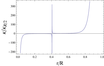
Figure 12: Isothermal compressibility as a function of the radial coordinate. $\kappa_{TR/2}$ stands for the thermal compressibility at $r/R=1/2$.

We can summarize the results of this section by asserting that the discontinuities in the second derivatives of the state functions (along with the continuity of the state functions and of their first derivative, as shown in the corresponding plots) indicate that the matter inside the black hole cannot be in thermodynamical equilibrium. This conclusion is reinforced by the plot of the transversal velocity as a function of the $r$, defined by:

$$v_{\perp}^{2}=\frac{dp_{\perp}}{d\rho}.$$

The function $v_{\perp}(r)$ can be calculated from (2) and (11). This function is plotted in Figure 13.

Figure 13: Tangential sound speed as a function of the radial coordinate.

The plot evidences not only the instability discussed above, but also a new one, inside the normal matter part of the object.

4.2 Dynamical equilibrium

To study the dynamical stability of the physical system inside the regular black hole, a detailed analysis of the Sturm-Liouville problem associated with the perturbation of the equations of motion for the fluid and the metric is mandatory. However, for the reasons discussed in the Appendix, we shall restrict ourselves here to some arguments suggesting that the system is dynamically unstable.

First, let us recall that in the region of exotic matter there is no propagation of sound waves. The equation for the radial sound speed, in the region of exotic matter, can be put as follows:

$$v_{r}^{2}=-\frac{\Delta p}{\Delta\rho}.$$ (33)

From (33) the pressure as a function of the density takes the form:

$$\Delta p=-v_{r}^{2}\Delta\rho,$$ (34)

where $v_{r}^{2}$ represents the square of the radial sound speed and it is always positive. We can see that if the pressure increases, the density decreases; but if the density decreases, the pressure keeps growing. In this process, both pressure and density are related in such a way by (34) that, if the system is perturbed, the fluid never stops expanding. We suggest that the huge accumulation of energy in this process of continuous expansion might lead to divergences that indicate the instability of the system.

5 Entropy of the gravitational field

Penrose p2 suggested that entropy might be assigned to the gravitational field itself and he proposed that the Weyl curvature tensor can be used to specify it.

A classical large-scale field such as gravity is expected to have associated an entropy as any other field that can be quantized and obeys the second law of thermodynamics, i.e. tends to a state of equilibrium. Of course, in the absence of a proper quantization of the field we cannot treat it as a gas of gravitons. Instead, we have to rely on approximate classical estimators. Since the equilibrium state of the field seems to be complete gravitational collapse, it appears reasonable to resort to classical estimators based on the Weyl tensor, i.e. the traceless part of the curvature tensor. Recent discussions of these topics are presented by Gr$\varnothing$n Gronsolo and by Clifton, Ellis, and Tavakol Ellis .

The behavior of the Weyl tensor follows what is expected for a gravitational entropy throughout the history of the universe: it is zero in the (homogeneous) Friedmann-Robertson-Walker model and it is large in Schwarzschild’s space-time.

Rudjord, Gr$\varnothing$n and Sigbj$\varnothing$rn Gron made a recent attempt to develop a quantitative classical description of the gravitational entropy based on the construction of a scalar derived from the contraction of the Weyl tensor and the Riemann tensor:

$$P^{2}=\dfrac{C^{\alpha\beta\gamma\delta}C_{\alpha\beta\gamma\delta}}{R^{\alpha\beta\gamma\delta}R_{\alpha\beta\gamma\delta}}=\frac{W}{K}.$$ (35)

This approach is based on matching their description of the entropy of a black hole in the event horizont with the Hawking-Bekenstein entropy bek . In particular, they calculated the entropy of Schwarzschild black holes and the Schwarzschild-de-Sitter space-time .

Rudjord et al. describe the gravitational entropy of a black hole by the surface integral:

$$S=k_{\rm{s}}\int_{\sigma}\vec{\Psi}\cdot\vec{d\sigma},$$ (36)

where $\sigma$ is the horizon of the black hole and the vector field $\vec{\Psi}$ is:

$$\vec{\Psi}=P\vec{e}_{r},$$ (37)

where $\vec{e}_{r}$ is a unitary vector in the radial direction. They required (36) to coincide at the horizon with the Hawking-Bekenstein entropy, thus allowing for the calculation of the constant $k_{\rm{s}}$.

Finally, the entropy density can be determined by means of Gauss’s divergence theorem, rewriting (36) as a volume integral:

$$\mathfrak{s}=k_{\rm{s}}\mid{\nabla\cdot\vec{\Psi}}\mid,$$ (38)

where the absolute value brackets were added to avoid negative values of entropy.

Let us recall that the Weyl tensor is the traceless part of the Riemann tensor, and is given by:

$$C_{\alpha\beta\gamma\delta} = R_{\alpha\beta\gamma\delta}+\frac{2}{n-2}(g_{\alpha[\gamma}R_{\delta]\beta}-g_{\beta[\gamma}R_{\delta]\alpha})+$$

$$+ \frac{2}{(n-1)(n-2)}R~{}g_{\alpha[\gamma}g_{\delta]\beta},$$

where $R_{\alpha\beta\gamma\delta}$ is the Riemann tensor, $R_{\alpha\beta}$ is the Ricci tensor, $R$ is the Ricci scalar, $[\ ]$ refers to the antisymmetric part, and $n$ is the number of dimensions of space-time.

The absence of structure in space-time corresponds to a null Weyl conformal curvature ($W=C^{abcd}C_{abcd}=0$). Hence, the Weyl tensor contains the information of the gravitational field in absence of matter and other non-gravitational fields.

The Weyl scalar for the space-time metric given in (1) is:

$$W = \frac{4}{3}\pi^{2}\rho^{2}_{\texttt{max}}(p_{\small{8}}\>x^{8}+p_{\small{6}}\>x^{6}+p_{\small{5}}\>x^{5}+p_{\small{4}}\>x^{4}+p_{\small{3}}\>x^{3}+p_{\small{2}}\>x^{2}+$$ (40)

$$+ p_{\small{1}}\>x+p_{\small{0}})^{2}/\left[\left(3r-\pi R^{3}\rho_{\rm{max}}+\pi R^{3}\rho_{\rm{max}}\>x\right)r^{6}R^{6}\right],$$

where $x=e^{-8\frac{r^{3}}{R^{3}}}$ and the coefficients $p_{\rm{i}}$ are:

$$p_{\small{0}} = 3R^{6}r-R^{9}\pi\rho_{\rm{max}},$$

$$p_{\small{1}} = 2R^{9}\pi\rho_{\rm{max}}-3R^{6}r+6r^{3}R^{6}\pi\rho_{\rm{max}}-24r^{4}R^{3},$$

$$p_{\small{2}} = -6r^{3}R^{6}\pi\rho_{\rm{max}}-R^{9}\pi\rho_{\rm{max}}+576r^{7}\alpha-$$

$$- 192r^{6}\alpha\pi R^{3}\rho_{\rm{max}}-2R^{6}r^{3}\alpha\pi\rho_{\rm{max}},$$

$$p_{\small{3}} = 2R^{6}r^{3}\alpha\pi\rho_{\rm{max}}+144r^{6}\alpha\pi R^{3}\rho_{\rm{max}},$$

$$p_{\small{4}} = (-1152-1152\alpha)r^{7}-48\pi R^{3}\rho_{\rm{max}}(-8\alpha-8+\alpha^{2})r^{6}+$$

$$+ 2\pi\rho_{\rm{max}}R^{6}(\alpha+1)r^{3},$$

$$p_{\small{5}} = -336\pi\rho_{\rm{max}}R^{3}(\alpha+1)r^{6}-2\pi\rho_{\rm{max}}R^{6}(\alpha+1)r^{3},$$

$$p_{\small{6}} = 96\pi\rho_{\rm{max}}\alpha R^{3}(\alpha+1)r^{6},$$

$$p_{\small{8}} = -48\pi R^{3}\rho_{\rm{max}}(\alpha+1)^{2}r^{6}.$$ (41)

If we let $r\rightarrow 0$, the Weyl scalar goes to zero. Since the regular black hole space-time has a de Sitter geometry in the origin, this is the expected limit.

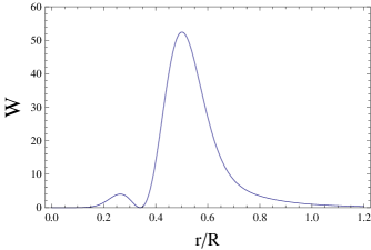
Figure 14: Weyl scalar as a function of the radial coordinate.

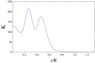
Figure 15: Kretschmann scalar as a function of the radial coordinate.

The plot of the Weyl scalar is shown in Figure 14. We see that for large values of $r$ the Weyl scalar tends asymptotically to zero. In the matter region ($r/R<1$) it has one absolute maximum at $r/R=0.5$ and one relative maximum at $r/R=0.26$. Between these points, $W=0$ at $r/R=0.34$. If we analyze the equation of state as a function of the density (Equation (2)), we find one inflexion point at $r/R=0.5$. The absolute maximum of the Weyl scalar seems to be related to the transition point between the two regions of matter.

The value of $r/R$ for which the Weyl scalar has one relative maximum is close to the point where the pressure is zero. This suggests a relation between the region where matter has a negative pressure and the behavior of the Weyl scalar. Notice that the inflexion point of the entropy density of the matter coincides with the value of $r/R$ for which the Weyl scalar is zero, that is at $r/R=0.34$. At this point the gravitational field changes from attractive to repulsive.

We also calculate the Kretschmann scalar. The plot is shown in Figure 15. Again, we see that outside the matter region the Kretschmann scalar tends asymptotically to zero. If we let $r\rightarrow 0$, it goes to:

$$K=\frac{512\pi^{2}{\rho_{\rm{max}}}^{2}}{3},$$ (42)

as expected for the de Sitter space-time. The Kretschmann scalar is always positive and it has one absolute maximum at $r/R=0.27$ and one relative maximum at $r/R=0.47$.

As a cross-check, we see from the plots that the calculated Weyl and Kretschmann scalars satisfy the relation:

$$R^{\alpha\beta\gamma\delta}R_{\alpha\beta\gamma\delta}\geq C^{\alpha\beta\gamma\delta}C_{\alpha\beta\gamma\delta},$$ (43)

that holds in every static spherically symmetric space-time Gron .

Figure 16: Gravitational entropy density as a function of the radial coordinate.

The gravitational entropy density of the MK model can be computed following following Rudjord et. al.’s proposal. The plot of the entropy density is shown in Figure 16. It is seen that $\mathfrak{s}=0$ at $r/R=0.27$, which is close to the transition point from positive to negative pressures. The absolute maximum is at $r/R=0.37$ and the two relative maxima are at $r/R=0.16$ and at $r/R=0.65$. For large values of $r/R$ the gravitational entropy density tends asymptotically to zero and in the core of the object it is also zero. This last result is in accordance with a correct classical description of the entropy of the gravitational field.

6 Conclusions

We have shown that the thermodynamical quantities describing the matter that is the source of the regular black hole model proposed by Mbonye and Kazanas indicate that the region of exotic matter is unstable. Some evidence has been presented that points to the dynamical instability of the model as well. The evidence for this second instability is supported by the plots of $v_{r}$ and $v_{\perp}$. In particular, the latter indicates the existence of a second type of dynamical instability, in the normal matter part of the object. These findings should be confirmed by a perturbation analysis (which will be presented elsewhere), based on the equations given in the Appendix.

We have also calculated the Weyl and Krestchmann scalars for the regular MK black hole, and a possible classical estimator of the gravitational entropy proposed by Rudjord, Gr$\varnothing$n and Sigbj$\varnothing$rn based on the Weyl curvature conjecture. It was shown that close to the core of the object, the entropy density tends to zero for large values of the radius. Hence, this classical estimator gives a good description of the entropy of the gravitational field in de Sitter and Schwarzschild limits.

Appendix: dynamical stability of the interior region

In order to study the stability of a system with tangential pressures against radial perturbations, both Einstein field equations and the equation of state must be perturbed following the standard procedure (see for instance hille ). The goal is to obtain a differential equation for the radial dependence of the quantity $\xi(r,t)$, which represents a small radial displacement of the fluid respect to its position of equilibrium at time $t$, that is, $r(r,t)=r_{0}+\xi(r,t).$

In what follows, the unperturbed metric coefficients $A(r)$, $B(r)$, and the unpertubed thermodynamics variables will be denoted by a zero subindex. The corresponding perturbations are denoted by $\delta A(r,t)$, $\delta B(r,t)$, $\delta p_{\text{r}}(r,t)$, $\delta p_{\perp}(r,t)$ and $\delta\rho(r,t)$. A long but straightforward calculation (which parallels that presented in hille ) shows that the equations for the perturbations are given by:

$$8\pi r^{2}\delta\rho = \frac{\partial}{\partial r}\left(\frac{r\delta A}{A_{0}^{2}}\right),$$ (44)

$$8\pi\dot{\xi}(\rho_{0}+p_{\text{r}}^{0}) = -\frac{1}{r}\frac{\partial\delta A}{\partial t}\frac{1}{A_{0}^{2}},$$ (45)

$$8\pi r^{2}\delta p_{\text{r}} = \frac{r}{A_{0}}\left[\frac{\partial}{\partial r}\left(\frac{\delta B}{B_{0}}\right)-\frac{dB_{0}}{dr}\frac{\delta A}{A_{0}}\right]-\frac{\delta A}{A_{0}^{2}},$$ (46)

$$\delta p_{\perp} = \frac{r}{2}\frac{\partial\delta p_{\text{r}}}{\partial r}+\delta p_{\text{r}}+\frac{r}{4B_{0}}\frac{dB_{0}}{dr}(\delta p_{\text{r}}+\delta\rho)$$ (47)

$$+\left[\frac{r}{4}\frac{\partial}{\partial r}\left(\frac{\delta B}{B_{0}}\right)+\frac{r}{2}\frac{A_{0}}{B_{0}}\frac{\partial^{2}\xi}{\partial t^{2}}\right](p_{\text{r}}^{0}+\rho_{0}).$$

Notice that there are six unknowns in this system, a consequence of the choices made by MK (one EOS and the explicit form of $\rho(r)$ to determine the system).

Equation (45) can be integrated respect to time , yielding:

$$\frac{\delta A}{A_{0}}=-8\pi r(\rho_{0}+p_{\text{r}}^{0})A_{0}\xi.$$ (48)

By isolating $\delta B$ from (46) we get:

$$\frac{\partial}{\partial r}\left(\frac{\delta B}{B_{0}}\right)=8\pi rA_{0}\delta p_{\text{r}}+\frac{\delta A}{A_{0}}\left(\frac{1}{B_{0}}\frac{dB_{0}}{dr}+\frac{1}{r}\right).$$ (49)

The final set of equations takes the form:

$$8\pi r^{2}\delta\rho = \frac{\partial}{\partial r}\left(\frac{r\delta A}{A_{0}^{2}}\right),$$ (50)

$$\delta p_{\text{r}}+(p_{\text{r}}^{0})^{\prime}\xi = \left(\frac{dp_{\text{r}}}{d\rho}\right)_{0}(\delta\rho+\rho_{0}^{\prime}\xi),$$ (51)

$$\delta p_{\perp} = \frac{r}{2}\frac{\partial\delta p_{\text{r}}}{\partial r}+\delta p_{\text{r}}+\frac{r}{4B_{0}}\frac{dB_{0}}{dr}(\delta p_{\text{r}}+\delta\rho)$$

$$+\left(\frac{r}{4}\frac{\partial}{\partial r}\left(\frac{\delta B}{B_{0}}\right)+\frac{r}{2}\frac{A_{0}}{B_{0}}\frac{\partial^{2}\xi}{\partial t^{2}}\right)(p_{\text{r}}^{0}+\rho_{0}),$$

$$\frac{\delta A}{A_{0}} = -8\pi r(\rho_{0}+p_{0})A_{0}\xi,$$ (53)

$$\frac{\partial}{\partial r}\left(\frac{\delta B}{B_{0}}\right) = 8\pi rA_{0}\delta p_{\textsf{r}}+\frac{\delta A}{A_{0}}\left(\frac{1}{B_{0}}\frac{dB_{0}}{dr}+\frac{1}{r}\right).$$ (54)

Standard manipulations using the expression $\xi(r,t)=\sigma(r)\exp{i\omega t}$ in these equations lead to the following second order ordinary inhomogeneous differential equation for the function $\sigma(r)$:

$$A_{\star}(r)\sigma^{\prime\prime}(r)+C_{\star}(r)\sigma^{\prime}(r)+\left[B_{\star}(r)+\omega D_{\star}(r)\right]\sigma(r)=\Pi(r),$$ (55)

where we have also used $\delta p_{\perp}(r,t)=\Pi(r)\exp{i\omega t}$.

This equation defines an inhomogeneous Sturm-Liouville (SL) problem, differently from the common case which yields a homogeneous one, the inhomogeneity being a direct consequence of the way the MK model solution was obtained, as mentioned before.

Equation (55) is to be solve for $r\in\left[0,1\right]$, using the boundary conditions $\sigma(r)=0$, $\sigma(1)=0$, and $\left[\delta\rho(1,t)+\rho^{\prime}_{0}(1,t)\xi(1,t)\right]=0$ hille . The coefficients $A_{\star}(r)$, $B_{\star}(r)$, $C_{\star}(r)$, and $D_{\star}(r)$ are given by:

$$A_{\star}(r)=\frac{r}{2}\left(p_{\text{r}}^{0}+\rho_{0}\right)\left(\frac{dp}{d\rho}\right)_{0},$$ (56)

$$B_{\star}(r)=B_{1}(r)+B_{2}(r)+B_{3}(r)+B_{4}(r),$$ (57)

where:

$$B_{1}(r) = \frac{1}{8\pi r^{2}}q^{\prime}(r)\alpha,$$ (58)

$$q^{\prime}(r) = \frac{\partial}{\partial r}\left[-8\pi r^{2}\left(\rho_{0}+p_{\text{r}}^{0}\right)\right],$$

$$\alpha = \frac{r}{2}\frac{\partial}{\partial r}\left(\frac{dp}{d\rho}\right)_{0}+\left(\frac{dp}{d\rho}\right)_{0}\Sigma(r)+\frac{r}{4B_{0}}\frac{dB_{0}}{dr},$$

$$\Sigma(r) = 1+\frac{r}{4B_{0}}\frac{dB_{0}}{dr}+4\pi r^{2}A_{0}\left(p_{\text{r}}^{0}+\rho_{0}\right),$$

$$B_{2}(r) = \frac{r}{2}\tau(r),$$ (59)

$$\tau(r) = \frac{\partial}{\partial r}\left(\frac{dp}{d\rho}\right)_{0}\rho^{\prime}_{0}-\frac{\partial}{\partial r}\left(p_{\text{r}}^{0}\right)^{\prime}+\left(\frac{dp}{d\rho}\right)_{0}\frac{\partial\rho^{\prime}_{0}}{\partial r},$$

$$B_{3}(r)=\frac{r}{2}\frac{\partial}{\partial r}\left(\frac{1}{8\pi r^{2}}q^{\prime}(r)\right)\left(\frac{dp}{d\rho}\right)_{0},$$ (60)

$$B_{4}(r)=-8\pi r\left(\rho_{0}+p_{\text{r}}^{0}\right)A_{0}\left[r\frac{d}{dr}\left(\ln B_{0}\right)+1\right],$$ (61)

$$C_{\star}(r)=C_{1}(r)+C_{2}(r)+C_{3}(r),$$ (62)

$$C_{1}(r) = \frac{1}{8\pi r^{2}}q\alpha,$$ (63)

$$q = -8\pi r^{2}\left(\rho_{0}+p_{\text{r}}^{0}\right),$$

$$C_{2}(r)=\frac{r}{2}\left[\left(\frac{dp}{d\rho}\right)_{0}\rho^{\prime}_{0}-p^{\prime}_{0}\right],$$ (64)

$$C_{3}(r)=\frac{1}{8\pi r}\left(-\frac{1}{r}q+q^{\prime}\right),$$ (65)

$$D_{\star}(r)=-\frac{r}{2}\frac{A_{0}}{B_{0}}\left(p_{\text{r}}^{0}+\rho_{0}\right).$$ (66)

For a given $\Pi(r)$, (55) might be solved using the Green’s function method (see for instance morse ). However, as we shall show next, the SL problem defined by (55) has a singular point. Consider the equation zettl :

$$-\left(py^{\prime}\right)^{\prime}+qy=\lambda wy,$$ (67)

which corresponds to the homogeneus SL problem defined on on $J=(a,b)$, with $-\infty\leq a\leq b\leq\infty$. The eigenvalue $\lambda$ is such that $\lambda\in\mathbb{C}$, and $p,q,w$ and $y$ are functions of $x$. It is also assumed that:

$$\frac{1}{p},q,w\in L_{{\rm loc}}\left(J,\mathbb{C}\right),$$ (68)

where $L_{{\rm loc}}\left(J,\mathbb{C}\right)$ denotes the linear manifold of functions $y$ satisfying $y\in L\left(\left[\alpha,\beta\right],\mathbb{C}\right)$ for all compact intervals $\left[\alpha,\beta\right]\subseteq J$. $L\left(J,\mathbb{C}\right)$ denotes the linear manifold of complex valued Lebesgue measurable functions $y$ defined on $J$ for which: $\int_{a}^{b}\left|y(t)\right|dt\equiv\int_{J}\left|y(t)\right|dt\equiv\int_{J}\left|y(t)\right|<\infty$.
Here $J$ is any interval of the real line, open, closed, half open, bounded or unbounded. Following zettl , we have the next definitions:

• The (finite or infinite) endpoint $a$ is regular if

  $$\frac{1}{p},q,w\in L((a,d),\mathbb{C}),$$ (69)

  holds for some (hence any) $d\in J$.

• An endpoint is called singular if it is not regular,

with similar definitions at $r=b$. To analyse whether $a=0$ is a regular or singular endpoint for our problem, defined by (55), we show in Figure 17 the plot of the coefficient $A_{\star}$ as a function of radial coordinate.

Figure 17: Coefficient $A_{\star}$ as a function of the radial coordinate.

We can see that $A_{\star}(0)=A_{\star}(0.4)=0$, $A_{\star}(r)<0$ for $r\in(0,0.4)$, and $A_{\star}(r)>0$ for $r\in(0.4,1)$. Hence, $\frac{1}{A}_{\star}\notin L((0,d),\mathbb{C})$ for any $d\in(0,1)$. Therefore, the endpoint $a=0$ is singular. If an endpoint is singular it could be a limit point or a limit circle. According to zettl , “there is hardly any literature on the LP/LC (limit point-limit circle) dichotomy when all three coefficients are present in the SL equation”. In particular, “there seems to be no literature on LP/LC criteria when $p$ changes sign”. Due to these complications, we shall attack this problem in a future publication.

References

- (1) Earman, J.:Bangs, crunches, whimpers and shrieks: singularities and acausalities in Relativistic Spacetimes. Oxford University Press, USA (1995)
- (2) Novello M., Perez Bergliaffa S. E.,: Bouncing cosmologies. Phys. Rept. 463, 127-213 (2008)
- (3) Markov, M. A.: Limiting density of matter as a universal law of nature. Pisḿa Zh. Eksp. Teor. Fiz. 36, 214-216 (1982)
- (4) Penrose R.: Gravitational collapse and space-time singularities. Phys. Rev. Lett. 14 57-59 (1965)
- (5) Hawking, S. W., Penrose, R: The singularities of gravitational collapse and cosmology. Proc. R. Soc. Lond. Mat. A 314 529-548 (1970)
- (6) Hawking, S. W., Ellis, G. R.: The cosmic black-body radiation and the existence of singularities in our universe. Astrophys. J. 152, 25-36 (1968)
- (7) Brandenberger, R. H., Mukhanov, V. F., Sornborger, A.: Cosmological theory without singularities. Phys. Rev. D 48, 1629-1642 (1993)
- (8) Gliner, E.: Algebraic properties of the energy-momentum tensor and vacuum-like states o+ matter. Sov. Phys.-JETP 22, 378 (1966)
- (9) Sakharov, A. D.: Expanding universe and the appearance of a nonuniform distribution of matter. Sov. Phys.-JETP 22, 241-249
- (10) Zeldovich, Y. B.: Special Issue: the cosmological constant and the theory of elementary particles. Sov. Phys. Usp. 11, 381-393 (1968)
- (11) Bardeen, J. M.: Non-singular general-relativistic gravitational collapse. Proc. of GR5, ed. V. A. Fock. Tbilisi University Press, Tbilisi p. 174 (1968)
- (12) Poisson, E., Israel, W.: Structure of the black hole nucleus. Class. Quantum Grav. 5 L201-L205 (1988)
- (13) Frolov, V. P., Markov, M. A., Mukhanov V. F.: Through a black hole into a new universe? Phys. Lett. B 216, 272-276 (1989)
- (14) Frolov, V. P., Markov, M. A., Mukhanov V. F.: Black holes as possible sources of closed and semiclosed worlds. Phys. Rev. D 41, 383-394 (1990)
- (15) Dymnikova, I.: Spherically symmetric space time with regular de sitter center. Int. J. Mod. Phys. D 12, 1015-1034 (2003)
- (16) Dymnikova, I.: Vacuum nonsingular black hole. Gen. Rel. Grav. 24, 235-242 (1992)
- (17) Mbonye, M. R., Kazanas, D.: Nonsingular black hole model as a possible end product of gravitational collapse. Phys. Rev. D 72 024016 (2005)
- (18) Lemos, J. P. S., Zanchin, V. T.: Regular black holes: Electrically charged solutions, Reissner-Nordstr m outside a de Sitter core. Phys. Rev. D 83, 124005 (2011)
- (19) Bronnikov, K. A., Fabris, J. C.: Regular phantom black holes. Phys. Rev. Lett. 96, 251101 (2006)
- (20) Bronnikov, K. A., Dehnen H., Melnikov, V. N.: Regular black holes and black universes. Gen. Rel. Grav. 39, 973-987 (2007)
- (21) Mbonye, M. R., Battista, N., Farr, B.: Time evolution of a non-singular primordial black hole. Int. J. Mod. Phys. D 20 1-18 (2011)
- (22) Saridakis E. N., González-Díaz P. F., Sig enza, C.: Unified dark energy thermodynamics: varying and the -1-crossing. Classical Quant. Grav. 26, 165003-165008 (2009)
- (23) Dymnikova, I., Korpusik, M.: Thermodynamics of regular cosmological black holes with de Sitter interior. Aip Conf. Proc. 17, 35-37 (2011). doi: 10.1134/S0202289311010075
- (24) Silva, R., Gonaçalves, R. S., Alcaniz, J. S., Silva H. H. B.: Thermodynamics and dark energy. A & A 576, A11 (2011). doi:10.1051/0004-6361/201117707
- (25) Rudjord, ., Grn, ., Sigbjrn, H.: The Weyl curvature conjecture and black hole entropy. Phys. Scr. 77, 055901 (2008)
- (26) Romero, G. E., Thomas, R., Pérez, D.: Gravitational entropy of black holes and wormholes. Int. J. Theor. Phys. 51, 925-942 (2012). doi: 10.1007/s10773-011-0967-8
- (27) Cattoen, C., Faber, T., Visser, M.: Gravastars must have anisotropic pressures. Class. Quantum Grav. 22, 4189-4202 (2005)
- (28) Horvat, D., Ilijic, S., Marunovic, A.: Radial stability analysis of the continuous pressure gravastar. Class. Quantum Grav. 28 025009 (2011)
- (29) Misner, C. W., Thorne, K. S., and Wheeler, J. A.:Gravitation. Freeman, San Francisco (1973)
- (30) Penrose, R.: Singularity and time-asymmetry in General Relativity, an Einstein centenary survey eds. S. W. Hawking, W. Israel. Cambridge Univ. Press, Cambridge pp 581-638 (1979)
- (31) Grn, .: Entropy and gravity. Entropy 14, 2456-2477 (2012)
- (32) Clifton, T., Ellis, G. F. R., Tavakol, R.: A gravitational entropy proposal. Class. Quantum Grav. 30, Issue 12, article id. 125009 (2013)
- (33) Bekenstein, J. D.: Generalized second law of thermodynamics in black-hole physics. Phys. Rev. D 9, 3292-3300 (1974)
- (34) Hillebrandt, W., Steinmetz, K.: Anisotropic neutron star models - Stability against radial and nonradial pulsations. A & A 53, 283-287 (1976)
- (35) Morse, M., Fesbach, M.: Methods of Theoretical Physics. Mc Graw-Hill Science, USA (1953)
- (36) Zettl, A.: Sturm-Liouville Theory. Mathematical Surveys and Monographs, Vol 121 American Mathematical Society (2005)