Degrees of freedom in lasso problems

Abstract

We derive the degrees of freedom of the lasso fit, placing no assumptions on the predictor matrix $X$. Like the well-known result of Zou, Hastie and Tibshirani [Ann. Statist. 35 (2007) 2173–2192], which gives the degrees of freedom of the lasso fit when $X$ has full column rank, we express our result in terms of the active set of a lasso solution. We extend this result to cover the degrees of freedom of the generalized lasso fit for an arbitrary predictor matrix $X$ (and an arbitrary penalty matrix $D$). Though our focus is degrees of freedom, we establish some intermediate results on the lasso and generalized lasso that may be interesting on their own.

and t1Supported by NSF Grant DMS-09-06801 and AFOSR Grant 113039.

1 Introduction

We study degrees of freedom, or the “effective number of parameters,” in $\ell_{1}$-penalized linear regression problems. In particular, for a response vector $y\in\mathbb{R}^{n}$, predictor matrix $X\in\mathbb{R}^{n\times p}$ and tuning parameter $\lambda\geq 0$, we consider the lasso problem [Chen, Donoho and Saunders (1998), Tibshirani (1996)]

$${\hat{\beta}}\in\mathop{{\operatorname{argmin}}}_{\beta\in\mathbb{R}^{p}}\frac{1}{2}\|y-X\beta\|_{2}^{2}+\lambda\|\beta\|_{1}.$$ (1)

The above notation emphasizes the fact that the solution ${\hat{\beta}}$ may not be unique [such nonuniqueness can occur if $\operatorname{rank}(X)<p$]. Throughout the paper, when a function $f\dvtx D\rightarrow\mathbb{R}^{n}$ may have a nonunique minimizer over its domain $D$, we write ${\operatorname{argmin}}_{x\in D}f(x)$ to denote the set of minimizing $x$ values, that is, ${\operatorname{argmin}}_{x\in D}f(x)=\{\hat{x}\in D\dvtx f(\hat{x})=\min_{x\in D}f(x)\}$.

A fundamental result on the degrees of freedom of the lasso fit was shown by Zou, Hastie and Tibshirani (2007). The authors show that if $y$ follows a normal distribution with spherical covariance, $y\sim N(\mu,\sigma^{2}I)$, and $X,\lambda$ are considered fixed with $\operatorname{rank}(X)=p$, then

$$\operatorname{df}(X{\hat{\beta}})=\mathrm{E}|{\mathcal{A}}|,$$ (2)

where ${\mathcal{A}}={\mathcal{A}}(y)$ denotes the active set of the unique lasso solution at $y$, and $|{\mathcal{A}}|$ is its cardinality. This is quite a well-known result, and is sometimes used to informally justify an application of the lasso procedure, as it says that number of parameters used by the lasso fit is simply equal to the (average) number of selected variables. However, we note that the assumption $\operatorname{rank}(X)=p$ implies that $p\leq n$; in other words, the degrees of freedom result (2) does not cover the important “high-dimensional” case $p>n$. In this case, the lasso solution is not necessarily unique, which raises the questions:

• Can we still express degrees of freedom in terms of the active set of a lasso solution?

• If so, which active set (solution) would we refer to?

In Section 3, we provide answers to these questions, by proving a stronger result when $X$ is a general predictor matrix. We show that the subspace spanned by the columns of $X$ in ${\mathcal{A}}$ is almost surely unique, where “almost surely” means for almost every $y\in\mathbb{R}^{n}$. Furthermore, the degrees of freedom of the lasso fit is simply the expected dimension of this column space.

We also consider the generalized lasso problem,

$${\hat{\beta}}\in\mathop{{\operatorname{argmin}}}_{\beta\in\mathbb{R}^{p}}\frac{1}{2}\|y-X\beta\|_{2}^{2}+\lambda\|D\beta\|_{1},$$ (3)

where $D\in\mathbb{R}^{m\times p}$ is a penalty matrix, and again the notation emphasizes the fact that ${\hat{\beta}}$ need not be unique [when $\operatorname{rank}(X)<p$]. This of course reduces to the usual lasso problem (1) when $D=I$, and Tibshirani and Taylor (2011) demonstrate that the formulation (3) encapsulates several other important problems—including the fused lasso on any graph and trend filtering of any order—by varying the penalty matrix $D$. The same paper shows that if $y$ is normally distributed as above, and $X,D,\lambda$ are fixed with $\operatorname{rank}(X)=p$, then the generalized lasso fit has degrees of freedom

$$\operatorname{df}(X{\hat{\beta}})=\mathrm{E}[\operatorname{nullity}(D_{-\mathcal{B}})].$$ (4)

Here $\mathcal{B}=\mathcal{B}(y)$ denotes the boundary set of an optimal subgradient to the generalized lasso problem at $y$ (equivalently, the boundary set of a dual solution at $y$), $D_{-\mathcal{B}}$ denotes the matrix $D$ after having removed the rows that are indexed by $\mathcal{B}$, and $\operatorname{nullity}(D_{-\mathcal{B}})=\operatorname{dim}(\operatorname{null}(D_{-\mathcal{B}}))$, the dimension of the null space of $D_{-\mathcal{B}}$.

It turns out that examining (4) for specific choices of $D$ produces a number of interpretable corollaries, as discussed in Tibshirani and Taylor (2011). For example, this result implies that the degrees of freedom of the fused lasso fit is equal to the expected number of fused groups, and that the degrees of freedom of the trend filtering fit is equal to the expected number of knots $+$ $(k-1)$, where $k$ is the order of the polynomial. The result (4) assumes that $\operatorname{rank}(X)=p$ and does not cover the case $p>n$; in Section 4, we derive the degrees of freedom of the generalized lasso fit for a general $X$ (and still a general $D$). As in the lasso case, we prove that there exists a linear subspace $X(\operatorname{null}(D_{-\mathcal{B}}))$ that is almost surely unique, meaning that it will be the same under different boundary sets $\mathcal{B}$ corresponding to different solutions of (3). The generalized lasso degrees of freedom is then the expected dimension of this subspace.

Our assumptions throughout the paper are minimal. As was already mentioned, we place no assumptions whatsoever on the predictor matrix $X\in\mathbb{R}^{n\times p}$ or on the penalty matrix $D\in\mathbb{R}^{m\times p}$, considering them fixed and nonrandom. We also consider $\lambda\geq 0$ fixed. For Theorems 1, 2 and 3 we assume that $y$ is normally distributed,

$$y\sim N(\mu,\sigma^{2}I)$$ (5)

for some (unknown) mean vector $\mu\in\mathbb{R}^{n}$ and marginal variance $\sigma^{2}\geq 0$. This assumption is only needed in order to apply Stein’s formula for degrees of freedom, and none of the other lasso and generalized lasso results in the paper, namely Lemmas 3 through 10, make any assumption about the distribution of $y$.

This paper is organized as follows. The rest of the Introduction contains an overview of related work, and an explanation of our notation. Section 2 covers some relevant background material on degrees of freedom and convex polyhedra. Though the connection may not be immediately obvious, the geometry of polyhedra plays a large role in understanding problems (1) and (3), and Section 2.2 gives a high-level view of this geometry before the technical arguments that follow in Sections 3 and 4. In Section 3, we derive two representations for the degrees of freedom of the lasso fit, given in Theorems 1 and 2. In Section 4, we derive the analogous results for the generalized lasso problem, and these are given in Theorem 3. As the lasso problem is a special case of the generalized lasso problem (corresponding to $D=I$), Theorems 1 and 2 can actually be viewed as corollaries of Theorem 3. The reader may then ask: why is there a separate section dedicated to the lasso problem? We give two reasons: first, the lasso arguments are simpler and easier to follow than their generalized lasso counterparts; second, we cover some intermediate results for the lasso problem that are interesting in their own right and that do not carry over to the generalized lasso perspective. Section 5 contains some final discussion.

1.1 Related work

All of the degrees of freedom results discussed here assume that the response vector has distribution $y\sim N(\mu,\sigma^{2}I)$, and that the predictor matrix $X$ is fixed. To the best of our knowledge, Efron et al. (2004) were the first to prove a result on the degrees of freedom of the lasso fit, using the lasso solution path with $\lambda$ moving from $\infty$ to $0$. The authors showed that when the active set reaches size $k$ along this path, the lasso fit has degrees of freedom exactly $k$. This result assumes that $X$ has full column rank and further satisfies a restrictive condition called the “positive cone condition,” which ensures that as $\lambda$ decreases, variables can only enter, and not leave, the active set. Subsequent results on the lasso degrees of freedom (including those presented in this paper) differ from this original result in that they derive degrees of freedom for a fixed value of the tuning parameter $\lambda$, and not a fixed number of steps $k$ taken along the solution path.

As mentioned previously, Zou, Hastie and Tibshirani (2007) established the basic lasso degrees of freedom result (for fixed $\lambda$) stated in (2). This is analogous to the path result of Efron et al. (2004); here degrees of freedom is equal to the expected size of the active set (rather than simply the size) because for a fixed $\lambda$ the active set is a random quantity, and can hence achieve a random size. The proof of (2) appearing in Zou, Hastie and Tibshirani (2007) relies heavily on properties of the lasso solution path. As also mentioned previously, Tibshirani and Taylor (2011) derived an extension of (2) to the generalized lasso problem, which is stated in (4) for an arbitrary penalty matrix $D$. Their arguments are not based on properties of the solution path, but instead come from a geometric perspective much like the one developed in this paper.

Both of the results (2) and (4) assume that $\operatorname{rank}(X)=p$; the current work extends these to the case of an arbitrary matrix $X$, in Theorems 1, 2 (the lasso) and 3 (the generalized lasso). In terms of our intermediate results, a version of Lemmas 5, 6 corresponding to $\operatorname{rank}(X)=p$ appears in Zou, Hastie and Tibshirani (2007), and a version of Lemma 9 corresponding to $\operatorname{rank}(X)=p$ appears in Tibshirani and Taylor (2011) [furthermore, Tibshirani and Taylor (2011) only consider the boundary set representation and not the active set representation]. Lemmas 1, 2 and the conclusions thereafter, on the degrees of freedom of the projection map onto a convex polyhedron, are essentially given in Meyer and Woodroofe (2000), though these authors state and prove the results in a different manner.

In preparing a draft of this manuscript, it was brought to our attention that other authors have independently and concurrently worked to extend results (2) and (4) to the general $X$ case. Namely, Dossal et al. (2011) prove a result on the lasso degrees of freedom, and Vaiter et al. (2011) prove a result on the generalized lasso degrees of freedom, both for an arbitrary $X$. These authors’ results express degrees of freedom in terms of the active sets of special (lasso or generalized lasso) solutions. Theorems 2 and 3 express degrees of freedom in terms of the active sets of any solutions, and hence the appropriate application of these theorems provides an alternative verification of these formulas. We discuss this in detail in the form of remarks following the theorems.

1.2 Notation

In this paper, we use $\operatorname{col}(A)$, $\operatorname{row}(A)$ and $\operatorname{null}(A)$ to denote the column space, row space and null space of a matrix $A$, respectively; we use $\operatorname{rank}(A)$ and $\operatorname{nullity}(A)$ to denote the dimensions of $\operatorname{col}(A)$ [equivalently, $\operatorname{row}(A)$] and $\operatorname{null}(A)$, respectively. We write $A^{+}$ for the the Moore–Penrose pseudoinverse of $A$; for a rectangular matrix $A$, recall that $A^{+}=(A^{T}A)^{+}A^{T}$. We write $P_{L}$ to denote the projection matrix onto a linear subspace $L$, and more generally, $P_{C}(x)$ to denote the projection of a point $x$ onto a closed convex set $C$. For readability, we sometimes write $\langle a,b\rangle$ (instead of $a^{T}b$) to denote the inner product between vectors $a$ and $b$.

For a set of indices $R=\{i_{1},\ldots,i_{k}\}\subseteq\{1,\ldots,m\}$ satisfying $i_{1}<\cdots<i_{k}$, and a vector $x\in\mathbb{R}^{m}$, we use $x_{R}$ to denote the subvector $x_{R}=(x_{i_{1}},\ldots,x_{i_{k}})^{T}\in\mathbb{R}^{k}$. We denote the complementary subvector by $x_{-R}=x_{\{1,\ldots,m\}\setminus R}\in\mathbb{R}^{m-k}$. The notation is similar for matrices. Given another subset of indices $S=\{j_{1},\ldots,j_{\ell}\}\subseteq\{1,\ldots,p\}$ with $j_{1}<\cdots<j_{\ell}$, and a matrix $A\in\mathbb{R}^{m\times p}$, we use $A_{(R,S)}$ to denote the submatrix

$$A_{(R,S)}=\left[\matrix{A_{i_{1},j_{1}}&\cdots&A_{i_{1},j_{\ell}}\cr\vdots&&\cr A_{i_{k},j_{1}}&\cdots&A_{i_{k},j_{\ell}}}\right]\in\mathbb{R}^{k\times\ell}.$$

In words, rows are indexed by $R$, and columns are indexed by $S$. When combining this notation with the transpose operation, we assume that the indexing happens first, so that $A_{(R,S)}^{T}=(A_{(R,S)})^{T}$. As above, negative signs are used to denote the complementary set of rows or columns; for example, $A_{(-R,S)}=A_{(\{1,\ldots,m\}\setminus R,S)}$. To extract only rows or only columns, we abbreviate the other dimension by a dot, so that $A_{(R,\cdot)}=A_{(R,\{1,\ldots,p\})}$ and $A_{(\cdot,S)}=A_{(\{1,\ldots,m\},S)}$; to extract a single row or column, we use $A_{(i,\cdot)}=A_{(\{i\},\cdot)}$ or $A_{(\cdot,j)}=A_{(\cdot,\{j\})}$. Finally, and most importantly, we introduce the following shorthand notation:

• For the predictor matrix $X\in\mathbb{R}^{n\times p}$, we let $X_{S}=X_{(\cdot,S)}$.

• For the penalty matrix $D\in\mathbb{R}^{m\times p}$, we let $D_{R}=D_{(R,\cdot)}$.

In other words, the default for $X$ is to index its columns, and the default for $D$ is to index its rows. This convention greatly simplifies the notation in expressions that involve multiple instances of $X_{S}$ or $D_{R}$; however, its use could also cause a great deal of confusion, if not properly interpreted by the reader!

2 Preliminary material

The following two sections describe some background material needed to follow the results in Sections 3 and 4.

2.1 Degrees of freedom

If the data vector $y\in\mathbb{R}^{n}$ is distributed according to the homoskedastic model $y\sim(\mu,\sigma^{2}I)$, meaning that the components of $y$ are uncorrelated, with $y_{i}$ having mean $\mu_{i}$ and variance $\sigma^{2}$ for $i=1,\ldots,n$, then the degrees of freedom of a function $g\dvtx\mathbb{R}^{n}\rightarrow\mathbb{R}^{n}$ with $g(y)=(g_{1}(y),\ldots,g_{n}(y))^{T}$, is defined as

$$\operatorname{df}(g)=\frac{1}{\sigma^{2}}\sum_{i=1}^{n}\operatorname{Cov}(g_{i}(y),y_{i}).$$ (6)

This definition is often attributed to Efron (1986) or Hastie and Tibshirani (1990), and is interpreted as the “effective number of parameters” used by the fitting procedure $g$. Note that for the linear regression fit of $y\in\mathbb{R}^{n}$ onto a fixed and full column rank predictor matrix $X\in\mathbb{R}^{n\times p}$, we have $g(y)=\hat{y}=XX^{+}y$, and $\operatorname{df}(\hat{y})=\operatorname{tr}(XX^{+})=p$, which is the number of fitted coefficients (one for each predictor variable). Furthermore, we can decompose the risk of $\hat{y}$, denoted by $\operatorname{Risk}(\hat{y})=\mathrm{E}\|\hat{y}-\mu\|_{2}^{2}$, as

$$\operatorname{Risk}(\hat{y})=\mathrm{E}\|\hat{y}-y\|_{2}^{2}-n\sigma^{2}+2p\sigma^{2},$$

a well-known identity that leads to the derivation of the $C_{p}$ statistic [Mallows (1973)]. For a general fitting procedure $g$, the motivation for the definition (6) comes from the analogous decomposition of the quantity $\operatorname{Risk}(g)=\mathrm{E}\|g(y)-\mu\|_{2}^{2}$,

$$\operatorname{Risk}(g)=\mathrm{E}\|g(y)-y\|_{2}^{2}-n\sigma^{2}+2\sum_{i=1}^{n}\operatorname{Cov}(g_{i}(y),y_{i}).$$ (7)

Therefore a large difference between risk and expected training error implies a large degrees of freedom.

Why is the concept of degrees of freedom important? One simple answer is that it provides a way to put different fitting procedures on equal footing. For example, it would not seem fair to compare a procedure that uses an effective number of parameters equal to 100 with another that uses only 10. However, assuming that these procedures can be tuned to varying levels of adaptivity (as is the case with the lasso and generalized lasso, where the adaptivity is controlled by $\lambda$), one could first tune the procedures to have the same degrees of freedom, and then compare their performances. Doing this over several common values for degrees of freedom may reveal, in an informal sense, that one procedure is particularly efficient when it comes to its parameter usage versus another.

A more detailed answer to the above question is based the risk decomposition (7). The decomposition suggests that an estimate $\widehat{\operatorname{df}}(g)$ of degrees of freedom can be used to form an estimate of the risk,

$$\widehat{\operatorname{Risk}}(g)=\|g(y)-y\|_{2}^{2}-n\sigma^{2}+2\sigma^{2}\widehat{\operatorname{df}}(g).$$ (8)

Furthermore, it is straightforward to check that an unbiased estimate of degrees of freedom leads to an unbiased estimate of risk; that is, $\operatorname{df}(g)=\mathrm{E}[\widehat{\operatorname{df}}(g)]$ implies $\operatorname{Risk}(g)=\mathrm{E}[\widehat{\operatorname{Risk}}(g)]$. Hence, the risk estimate (8) can be used to choose between fitting procedures, assuming that unbiased estimates of degrees of freedom are available. [It is worth mentioning that bootstrap or Monte Carlo methods can be helpful in estimating degrees of freedom (6) when an analytic form is difficult to obtain.] The natural extension of this idea is to use the risk estimate (8) for tuning parameter selection. If we suppose that $g$ depends on a tuning parameter $\lambda\in\Lambda$, denoted $g=g_{\lambda}(y)$, then in principle one could minimize the estimated risk over $\lambda$ to select an appropriate value for the tuning parameter,

$$\hat{\lambda}=\mathop{{\operatorname{argmin}}}_{\lambda\in\Lambda}\|g_{\lambda}(y)-y\|_{2}^{2}-n\sigma^{2}+2\sigma^{2}\widehat{\operatorname{df}}(g_{\lambda}).$$ (9)

This is a computationally efficient alternative to selecting the tuning parameter by cross-validation, and it is commonly used (along with similar methods that replace the factor of $2$ above with a function of $n$ or $p$) in penalized regression problems. Even though such an estimate (9) is commonly used in the high-dimensional setting ($p>n$), its asymptotic properties are largely unknown in this case, such as risk consistency, or relatively efficiency compared to the cross-validation estimate.

Stein (1981) proposed the risk estimate (8) using a particular unbiased estimate of degrees of freedom, now commonly referred to as Stein’s unbiased risk estimate (SURE). Stein’s framework requires that we strengthen our distributional assumption on $y$ and assume normality, as stated in (5). We also assume that the function $g$ is continuous and almost differentiable. (The precise definition of almost differentiability is not important here, but the interested reader may take it to mean that each coordinate function $g_{i}$ is absolutely continuous on almost every line segment parallel to one of the coordinate axes.) Given these assumptions, Stein’s main result is an alternate expression for degrees of freedom,

$$\operatorname{df}(g)=\mathrm{E}[(\nabla\cdot g)(y)],$$ (10)

where the function $\nabla\cdot g=\sum_{i=1}^{n}\partial g_{i}/\partial y_{i}$ is called the divergence of $g$. Immediately following is the unbiased estimate of degrees of freedom,

$$\widehat{\operatorname{df}}(g)=(\nabla\cdot g)(y).$$ (11)

We pause for a moment to reflect on the importance of this result. From its definition (6), we can see that the two most obvious candidates for unbiased estimates of degrees of freedom are

$$\frac{1}{\sigma^{2}}\sum_{i=1}^{n}g_{i}(y)(y_{i}-\mu_{i})\quad\mbox{and}\quad\frac{1}{\sigma^{2}}\sum_{i=1}^{n}\bigl{(}g_{i}(y)-\mathrm{E}[g_{i}(y)]\bigr{)}y_{i}.$$

To use the first estimate above, we need to know $\mu$ (remember, this is ultimately what we are trying to estimate!). Using the second requires knowing $\mathrm{E}[g(y)]$, which is equally impractical because this invariably depends on $\mu$. On the other hand, Stein’s unbiased estimate (11) does not have an explicit dependence on $\mu$; moreover, it can be analytically computed for many fitting procedures $g$. For example, Theorem 2 in Section 3 shows that, except for $y$ in a set of measure zero, the divergence of the lasso fit is equal to $\operatorname{rank}(X_{\mathcal{A}})$ with ${\mathcal{A}}={\mathcal{A}}(y)$ being the active set of a lasso solution at $y$. Hence, Stein’s formula allows for the unbiased estimation of degrees of freedom (and subsequently, risk) for a broad class of fitting procedures $g$—something that may have not seemed possible when working from the definition directly.

2.2 Projections onto polyhedra

A set $C\subseteq\mathbb{R}^{n}$ is called a convex polyhedron, or simply a polyhedron, if $C$ is the intersection of finitely many half-spaces,

$$C=\bigcap_{i=1}^{k}\{x\in\mathbb{R}^{n}\dvtx a_{i}^{T}x\leq b_{i}\},$$ (12)

where $a_{1},\ldots,a_{k}\in\mathbb{R}^{n}$ and $b_{1},\ldots,b_{k}\in\mathbb{R}$. (Note that we do not require boundedness here; a bounded polyhedron is sometimes called a polytope.) See Figure 1 for an example. There is a rich theory on polyhedra; the definitive reference is Grünbaum (2003), and another good reference is Schneider (1993). As this is a paper on statistics and not geometry, we do not attempt to give an extensive treatment of the properties of polyhedra. We do, however, give two properties (in the form of two lemmas) that are especially important with respect to our statistical problem; our discussion will also make it clear why polyhedra are relevant in the first place.

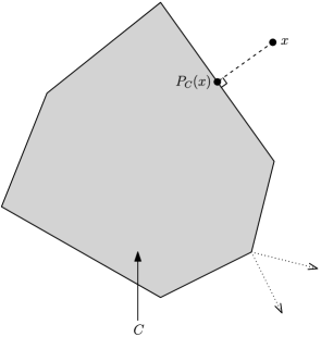
Figure 1: An example of a polyhedron in $\mathbb{R}^{2}$.

From its definition (12), it follows that a polyhedron is a closed convex set. The first property that we discuss does not actually rely on the special structure of polyhedra, but only on convexity. For any closed convex set $C\subseteq\mathbb{R}^{n}$ and any point $x\in\mathbb{R}^{n}$, there is a unique point $u\in C$ minimizing $\|x-u\|_{2}$. To see this, note that if $v\in C$ is another minimizer, $v\not=u$, then by convexity $w=(u+v)/2\in C$, and $\|x-w\|_{2}<\|x-u\|_{2}/2+\|x-v\|_{2}/2=\|x-u\|_{2}$, a contradiction. Therefore, the projection map onto $C$ is indeed well defined, and we write this as $P_{C}\dvtx\mathbb{R}^{n}\rightarrow C$,

$$P_{C}(x)=\mathop{{\operatorname{argmin}}}_{u\in C}\|x-u\|_{2}.$$

For the usual linear regression problem, where $y\in\mathbb{R}^{n}$ is regressed onto $X\in\mathbb{R}^{n\times p}$, the fit $X{\hat{\beta}}$ can be written in terms of the projection map onto the polyhedron $C=\operatorname{col}(X)$, as in $X{\hat{\beta}}(y)=XX^{+}y=P_{\operatorname{col}(X)}(y)$. Furthermore, for both the lasso and generalized lasso problems, (1) and (3), it turns out that we can express the fit as the residual from projecting onto a suitable polyhedron $C\subseteq\mathbb{R}^{n}$, that is,

$$X{\hat{\beta}}(y)=(I-P_{C})(y)=y-P_{C}(y).$$

This is proved in Lemma 3 for the lasso and in Lemma 8 for the generalized lasso (the polyhedron $C$ depends on $X,\lambda$ for the lasso case, and on $X,D,\lambda$ for the generalized lasso case). Our first lemma establishes that both the projection map onto a closed convex set and the residual map are nonexpansive, hence continuous and almost differentiable everywhere. These are the conditions needed to apply Stein’s formula.

Lemma 1

For any closed convex set $C\subseteq\mathbb{R}^{n}$, both the projection map $P_{C}\dvtx\mathbb{R}^{n}\rightarrow C$ and the residual projection map $I-P_{C}\dvtx\mathbb{R}^{n}\rightarrow\mathbb{R}^{n}$ are nonexpansive. That is, they satisfy

$$\|P_{C}(x)-\mathrm{P}_{C}(y)\|_{2} \leq \|x-y\|_{2}\qquad\mbox{for any }x,y\in\mathbb{R}^{n},\quad\mbox{and}$$

$$\|(I-P_{C})(x)-(I-P_{C})(y)\|_{2} \leq \|x-y\|_{2}\qquad\mbox{for any }x,y\in\mathbb{R}^{n}.$$

Therefore, $P_{C}$ and $I-P_{C}$ are both continuous and almost differentiable.

The proof can be found in Appendix A.1. Lemma 1 will be quite useful later in the paper, as it will allow us to use Stein’s formula to compute the degrees of freedom of the lasso and generalized lasso fits, after showing that these fits are indeed the residuals from projecting onto closed convex sets.

The second property that we discuss uses the structure of polyhedra. Unlike Lemma 1, this property will not be used directly in the following sections of the paper; instead, we present it here to give some intuition with respect to the degrees of freedom calculations to come. The property can be best explained by looking back at Figure 1. Loosely speaking, the picture suggests that we can move the point $x$ around a bit and it will still project to the same face of $C$. Another way of saying this is that there is a neighborhood of $x$ on which $P_{C}$ is simply the projection onto an affine subspace. This would not be true if $x$ is in some exceptional set, which is made up of rays that emanate from the corners of $C$, like the two drawn in the bottom right corner of figure. However, the union of such rays has measure zero, so the map $P_{C}$ is locally an affine projection, almost everywhere. This idea can be stated formally as follows.

Lemma 2

Let $C\subseteq\mathbb{R}^{n}$ be a polyhedron. For almost every $x\in\mathbb{R}^{n}$, there is an associated neighborhood $U$ of $x$, linear subspace $L\subseteq\mathbb{R}^{n}$ and point $a\in\mathbb{R}^{n}$, such that the projection map restricted to $U$, $P_{C}\dvtx U\rightarrow C$, is

$$P_{C}(y)=P_{L}(y-a)+a\qquad\mbox{for }y\in U,$$

which is simply the projection onto the affine subspace $L+a$.

The proof is given in Appendix A.2. These last two properties can be used to derive a general expression for the degrees of freedom of the fitting procedure $g(y)=(I-P_{C})(y)$, when $C\subseteq\mathbb{R}^{n}$ is a polyhedron. [A similar formula holds for $g(y)=P_{C}(y)$.] Lemma 1 tells us that $I-P_{C}$ is continuous and almost differentiable, so we can use Stein’s formula (10) to compute its degrees of freedom. Lemma 2 tells us that for almost every $y\in\mathbb{R}^{n}$, there is a neighborhood $U$ of $y$, linear subspace $L\subseteq\mathbb{R}^{n}$, and point $a\in\mathbb{R}^{n}$, such that

$$(I-P_{C})(y^{\prime})=y^{\prime}-P_{L}(y^{\prime}-a)-a=(I-P_{L})(y^{\prime}-a)\qquad\mbox{for }y^{\prime}\in U.$$

Therefore,

$$\bigl{(}\nabla\cdot(I-P_{C})\bigr{)}(y)=\operatorname{tr}(I-P_{L})=n-\operatorname{dim}(L),$$

and an expectation over $y$ gives

$$\operatorname{df}(I-P_{C})=n-\mathrm{E}[\operatorname{dim}(L)].$$

It should be made clear that the random quantity in the above expectation is the linear subspace $L=L(y)$, which depends on $y$.

In a sense, the remainder of this paper is focused on describing $\operatorname{dim}(L)$—the dimension of the face of $C$ onto which the point $y$ projects—in a meaningful way for the lasso and generalized lasso problems. Section 3 considers the lasso problem, and we show that $L$ can be written in terms of the equicorrelation set of the fit at $y$. We also show that $L$ can be described in terms of the active set of a solution at $y$. In Section 4 we show the analogous results for the generalized lasso problem, namely, that $L$ can be written in terms of either the boundary set of an optimal subgradient at $y$ (the analogy of the equicorrelation set for the lasso) or the active set of a solution at $y$.

3 The lasso

In this section we derive the degrees of freedom of the lasso fit, for a general predictor matrix $X$. All of our arguments stem from the Karush–Kuhn–Tucker (KKT) optimality conditions, and we present these first. We note that many of the results in this section can be alternatively derived using the lasso dual problem. Appendix A.5 explains this connection more precisely. For the current work, we avoid the dual perspective simply to keep the presentation more self-contained. Finally, we remind the reader that $X_{S}$ is used to extract columns of $X$ corresponding to an index set $S$.

3.1 The KKT conditions and the underlying polyhedron

The KKT conditions for the lasso problem (1) can be expressed as

$$\displaystyle X^{T}(y-X{\hat{\beta}})=\lambda\gamma,$$ (13)

$$\displaystyle\gamma_{i}\in\cases{\{\operatorname{sign}({\hat{\beta}}_{i})\}&\quad if ${\hat{\beta}}_{i}\not=0$,\vspace*{2pt}\cr[-1,1]&\quad if ${\hat{\beta}}_{i}=0$.}$$ (14)

Here $\gamma\in\mathbb{R}^{p}$ is a subgradient of the function $f(x)=\|x\|_{1}$ evaluated at $x={\hat{\beta}}$. Hence ${\hat{\beta}}$ is a minimizer in (1) if and only if ${\hat{\beta}}$ satisfies (13) and (14) for some $\gamma$. Directly from the KKT conditions, we can show that $X{\hat{\beta}}$ is the residual from projecting $y$ onto a polyhedron.

Lemma 3

For any $X$ and $\lambda\geq 0$, the lasso fit $X{\hat{\beta}}$ can be written as $X{\hat{\beta}}(y)=(I-P_{C})(y)$, where $C\subseteq\mathbb{R}^{n}$ is the polyhedron

$$C=\{u\in\mathbb{R}^{n}\dvtx\|X^{T}u\|_{\infty}\leq\lambda\}.$$

Given a point $y\in\mathbb{R}^{n}$, its projection $\theta=P_{C}(y)$ onto a closed convex set $C\subseteq\mathbb{R}^{n}$ can be characterized as the unique point satisfying

$$\langle y-\theta,\theta-u\rangle\geq 0\qquad\mbox{for all }u\in C.$$ (15)

Hence defining $\theta=y-X{\hat{\beta}}(y)$, and $C$ as in the lemma, we want to show that (15) holds for all $u\in C$. Well,

$$\langle y-\theta,\theta-u\rangle = \langle X{\hat{\beta}},y-X{\hat{\beta}}-u\rangle$$

$$= \langle X{\hat{\beta}},y-X{\hat{\beta}}\rangle-\langle X^{T}u,{\hat{\beta}}\rangle.$$

Consider the first term above. Taking an inner product with ${\hat{\beta}}$ on both sides of (13) gives $\langle X{\hat{\beta}},y-X{\hat{\beta}}\rangle=\lambda\|{\hat{\beta}}\|_{1}$. Furthermore, the $\ell_{1}$ norm can be characterized in terms of its dual norm, the $\ell_{\infty}$ norm, as in

$$\lambda\|{\hat{\beta}}\|_{1}=\max_{\|w\|_{\infty}\leq\lambda}\langle w,{\hat{\beta}}\rangle.$$

Therefore, continuing from (3.1), we have

$$\langle y-\theta,\theta-u\rangle=\max_{\|w\|_{\infty}\leq\lambda}\langle w,{\hat{\beta}}\rangle-\langle X^{T}u,{\hat{\beta}}\rangle,$$

which is $\geq 0$ for all $u\in C$, and we have hence proved that $\theta=y-X{\hat{\beta}}(y)=P_{C}(y)$. To show that $C$ is indeed a polyhedron, note that it can be written as

$$C=\bigcap_{i=1}^{p}(\{u\in\mathbb{R}^{n}\dvtx X_{i}^{T}u\leq\lambda\}\cap\{u\in\mathbb{R}^{n}\dvtx X_{i}^{T}u\geq-\lambda\}),$$

which is a finite intersection of half-spaces.

Showing that the lasso fit is the residual from projecting $y$ onto a polyhedron is important, because it means that $X{\hat{\beta}}(y)$ is nonexpansive as a function of $y$, and hence continuous and almost differentiable, by Lemma 1. This establishes the conditions that are needed to apply Stein’s formula for degrees of freedom.

In the next section, we define the equicorrelation set $\mathcal{E}$, and show that the lasso fit and solutions both have an explicit form in terms of $\mathcal{E}$. Following this, we derive an expression for the lasso degrees of freedom as a function of the equicorrelation set.

3.2 The equicorrelation set

According to Lemma 3, the lasso fit $X{\hat{\beta}}$ is always unique (because projection onto a closed convex set is unique). Therefore, even though the solution ${\hat{\beta}}$ is not necessarily unique, the optimal subgradient $\gamma$ is unique, because it can be written entirely in terms of $X{\hat{\beta}}$, as shown by (13). We define the unique equicorrelation set $\mathcal{E}$ as

$$\mathcal{E}=\{i\in\{1,\ldots,p\}\dvtx|\gamma_{i}|=1\}.$$ (17)

An alternative definition for the equicorrelation set is

$$\mathcal{E}=\{i\in\{1,\ldots,p\}\dvtx|X_{i}^{T}(y-X{\hat{\beta}})|=\lambda\},$$ (18)

which explains its name, as $\mathcal{E}$ can be thought of as the set of variables that have equal and maximal absolute inner product (or correlation for standardized variables) with the residual.

The set $\mathcal{E}$ is a natural quantity to work with because we can express the lasso fit and the set of lasso solutions in terms of $\mathcal{E}$, by working directly from equation (13). First we let

$$s=\operatorname{sign}(\gamma_{\mathcal{E}})=\operatorname{sign}\bigl{(}X_{\mathcal{E}}^{T}(y-X{\hat{\beta}})\bigr{)},$$ (19)

the signs of the inner products of the equicorrelation variables with the residual. Since ${\hat{\beta}}_{-\mathcal{E}}=0$ by definition of the subgradient, the $\mathcal{E}$ block of the KKT conditions can be rewritten as

$$X_{\mathcal{E}}^{T}(y-X_{\mathcal{E}}{\hat{\beta}}_{\mathcal{E}})=\lambda s.$$ (20)

Because $\lambda s\in\operatorname{row}(X_{\mathcal{E}})$, we can write $\lambda s=X_{\mathcal{E}}^{T}(X_{\mathcal{E}}^{T})^{+}\lambda s$, so rearranging (20) we get

$$X_{\mathcal{E}}^{T}X_{\mathcal{E}}{\hat{\beta}}_{\mathcal{E}}=X_{\mathcal{E}}^{T}\bigl{(}y-(X_{\mathcal{E}}^{T})^{+}\lambda s\bigr{)}.$$

Therefore, the lasso fit $X{\hat{\beta}}=X_{\mathcal{E}}{\hat{\beta}}_{\mathcal{E}}$ is

$$X{\hat{\beta}}=X_{\mathcal{E}}(X_{\mathcal{E}})^{+}\bigl{(}y-(X_{\mathcal{E}}^{T})^{+}\lambda s\bigr{)},$$ (21)

and any lasso solution must be of the form

$${\hat{\beta}}_{-\mathcal{E}}=0\quad\mbox{and}\quad{\hat{\beta}}_{\mathcal{E}}=(X_{\mathcal{E}})^{+}\bigl{(}y-(X_{\mathcal{E}}^{T})^{+}\lambda s\bigr{)}+b,$$ (22)

where $b\in\operatorname{null}(X_{\mathcal{E}})$. In the case that $\operatorname{null}(X_{\mathcal{E}})=\{0\}$—for example, this holds if $\operatorname{rank}(X)=p$—the lasso solution is unique and is given by (22) with $b=0$. But in general, when $\operatorname{null}(X_{\mathcal{E}})\not=\{0\}$, it is important to note that not every $b\in\operatorname{null}(X_{\mathcal{E}})$ necessarily leads to a lasso solution in (22); the vector $b$ must also preserve the signs of the nonzero coefficients; that is, it must also satisfy

$$\operatorname{sign}\bigl{(}\bigl{[}(X_{\mathcal{E}})^{+}\bigl{(}y-(X_{\mathcal{E}}^{T})^{+}\lambda s\bigr{)}\bigr{]}_{i}+b_{i}\bigr{)}=s_{i}$$

(23)

$$\eqntext{\mbox{for each $i$ such that }\bigl{[}(X_{\mathcal{E}})^{+}\bigl{(}y-(X_{\mathcal{E}}^{T})^{+}\lambda s\bigr{)}\bigr{]}_{i}+b_{i}\not=0.}$$ (24)

Otherwise, $\gamma$ would not be a proper subgradient of $\|{\hat{\beta}}\|_{1}$.

3.3 Degrees of freedom in terms of the equicorrelation set

Using relatively simple arguments, we can derive a result on the lasso degrees of freedom in terms of the equicorrelation set. Our arguments build on the following key lemma.

Lemma 4

For any $y,X$ and $\lambda\geq 0$, a lasso solution is given by

$${\hat{\beta}}_{-\mathcal{E}}=0\quad\mbox{and}\quad{\hat{\beta}}_{\mathcal{E}}=(X_{\mathcal{E}})^{+}\bigl{(}y-(X_{\mathcal{E}}^{T})^{+}\lambda s\bigr{)},$$ (25)

where $\mathcal{E}$ and $s$ are the equicorrelation set and signs, as defined in (17) and (19).

In other words, Lemma 4 says that the sign condition (3.2) is always satisfied by taking $b=0$, regardless of the rank of $X$. This result is inspired by the LARS work of Efron et al. (2004), though it is not proved in the LARS paper; see Appendix B of Tibshirani (2011) for a proof.

Next we show that, almost everywhere in $y$, the equicorrelation set and signs are locally constant functions of $y$. To emphasize their functional dependence on $y$, we write them as $\mathcal{E}(y)$ and $s(y)$.

Lemma 5

For almost every $y\in\mathbb{R}^{n}$, there exists a neighborhood $U$ of $y$ such that $\mathcal{E}(y^{\prime})=\mathcal{E}(y)$ and $s(y)=s(y^{\prime})$ for all $y^{\prime}\in U$.

Define

$$\mathcal{N}=\bigcup_{\mathcal{E},s}\bigcup_{i\in\mathcal{E}}\bigl{\{}z\in\mathbb{R}^{n}\dvtx[(X_{\mathcal{E}})^{+}]_{(i,\cdot)}\bigl{(}z-(X_{\mathcal{E}}^{T})^{+}\lambda s\bigr{)}=0\bigr{\}},$$

where the first union above is taken over all subsets $\mathcal{E}\subseteq\{1,\ldots,p\}$ and sign vectors $s\in\{-1,1\}^{|\mathcal{E}|}$, but we exclude sets $\mathcal{E}$ for which a row of $(X_{\mathcal{E}})^{+}$ is entirely zero. The set $\mathcal{N}$ is a finite union of affine subspaces of dimension $n-1$, and therefore has measure zero.

Let $y\notin\mathcal{N}$, and abbreviate the equicorrelation set and signs as $\mathcal{E}=\mathcal{E}(y)$ and $s=s(y)$. We may assume no row of $(X_{\mathcal{E}})^{+}$ is entirely zero. (Otherwise, this implies that $X_{\mathcal{E}}$ has a zero column, which implies that $\lambda=0$, a trivial case for this lemma.) Therefore, as $y\notin\mathcal{N}$, this means that the lasso solution given in (25) satisfies ${\hat{\beta}}_{i}(y)\not=0$ for every $i\in\mathcal{E}$.

Now, for a new point $y^{\prime}$, consider defining

$${\hat{\beta}}_{-\mathcal{E}}(y^{\prime})=0\quad\mbox{and}\quad{\hat{\beta}}_{\mathcal{E}}(y^{\prime})=(X_{\mathcal{E}})^{+}\bigl{(}y^{\prime}-(X_{\mathcal{E}}^{T})^{+}\lambda s\bigr{)}.$$

We need to verify that this is indeed a solution at $y^{\prime}$, and that the corresponding fit has equicorrelation set $\mathcal{E}$ and signs $s$. First notice that, after a straightforward calculation,

$$X_{\mathcal{E}}^{T}\bigl{(}y^{\prime}-X{\hat{\beta}}(y^{\prime})\bigr{)}=X_{\mathcal{E}}^{T}\bigl{(}y^{\prime}-X_{\mathcal{E}}(X_{\mathcal{E}})^{+}\bigl{(}y^{\prime}-(X_{\mathcal{E}}^{T})^{+}\lambda s\bigr{)}\bigr{)}=\lambda s.$$

Also, by the continuity of the function $f\dvtx\mathbb{R}^{n}\rightarrow\mathbb{R}^{p-|\mathcal{E}|}$,

$$f(x)=X_{-\mathcal{E}}^{T}\bigl{(}x-X_{\mathcal{E}}(X_{\mathcal{E}})^{+}\bigl{(}x-(X_{\mathcal{E}}^{T})^{+}\lambda s\bigr{)}\bigr{)},$$

there exists a neighborhood $U_{1}$ of $y$ such that

$$\bigl{\|}X_{-\mathcal{E}}^{T}\bigl{(}y^{\prime}-X{\hat{\beta}}(y^{\prime})\bigr{)}\bigr{\|}_{\infty}=\bigl{\|}X_{-\mathcal{E}}^{T}\bigl{(}y^{\prime}-X_{\mathcal{E}}(X_{\mathcal{E}})^{+}\bigl{(}y^{\prime}-(X_{\mathcal{E}}^{T})^{+}\lambda s\bigr{)}\bigr{)}\bigr{\|}_{\infty}<\lambda$$

for all $y^{\prime}\in U_{1}$. Hence $X{\hat{\beta}}(y^{\prime})$ has equicorrelation set $\mathcal{E}(y^{\prime})=\mathcal{E}$ and signs $s(y^{\prime})=s$.

To check that ${\hat{\beta}}(y^{\prime})$ is a lasso solution at $y^{\prime}$, we consider the function $g\dvtx\mathbb{R}^{n}\rightarrow\mathbb{R}^{|\mathcal{E}|}$,

$$g(x)=(X_{\mathcal{E}})^{+}\bigl{(}x-(X_{\mathcal{E}}^{T})^{+}\lambda s\bigr{)}.$$

The continuity of $g$ implies that there exists a neighborhood $U_{2}$ of $y$ such that

$${\hat{\beta}}_{i}(y^{\prime}) = \bigl{[}(X_{\mathcal{E}}^{T})^{+}\bigl{(}y^{\prime}-(X_{\mathcal{E}}^{T})^{+}\lambda s\bigr{)}\bigr{]}_{i}\not=0\qquad\mbox{for }i\in\mathcal{E},\quad\mbox{and}$$

$$\operatorname{sign}({\hat{\beta}}_{\mathcal{E}}(y^{\prime})) = \operatorname{sign}\bigl{(}(X_{\mathcal{E}})^{+}\bigl{(}y^{\prime}-(X_{\mathcal{E}}^{T})^{+}\lambda s\bigr{)}\bigr{)}$$

for each $y^{\prime}\in U_{2}$. Defining $U=U_{1}\cap U_{2}$ completes the proof.

This immediately implies the following theorem.

Theorem 1 ((Lasso degrees of freedom, equicorrelation set representation))

Assume that $y$ follows a normal distribution (5). For any $X$ and $\lambda\geq 0$, the lasso fit $X{\hat{\beta}}$ has degrees of freedom

$$\operatorname{df}(X{\hat{\beta}})=\mathrm{E}[\operatorname{rank}(X_{\mathcal{E}})],$$

where $\mathcal{E}=\mathcal{E}(y)$ is the equicorrelation set of the lasso fit at $y$.

By Lemmas 1 and 3 we know that $X{\hat{\beta}}(y)$ is continuous and almost differentiable, so we can use Stein’s formula (10) for degrees of freedom. By Lemma 5, we know that $\mathcal{E}=\mathcal{E}(y)$ and $s=s(y)$ are locally constant for all $y\notin\mathcal{N}$. Therefore, taking the divergence of the fit in (21), we get

$$(\nabla\cdot X{\hat{\beta}})(y)=\operatorname{tr}(X_{\mathcal{E}}(X_{\mathcal{E}})^{+})=\operatorname{rank}(X_{\mathcal{E}}).$$

Taking an expectation over $y$ (and recalling that $\mathcal{N}$ has measure zero) gives the result.

Next, we shift our focus to a different subset of variables: the active set ${\mathcal{A}}$. Unlike the equicorrelation set, the active set is not unique, as it depends on a particular choice of lasso solution. Though it may seem that such nonuniqueness could present complications, it turns out that all of the active sets share a special property; namely, the linear subspace $\operatorname{col}(X_{\mathcal{A}})$ is the same for any choice of active set ${\mathcal{A}}$, almost everywhere in $y$. This invariance allows us to express the degrees of freedom of lasso fit in terms of the active set (or, more precisely, any active set).

3.4 The active set

Given a particular solution ${\hat{\beta}}$, we define the active set ${\mathcal{A}}$ as

$${\mathcal{A}}=\bigl{\{}i\in\{1,\ldots,p\}\dvtx{\hat{\beta}}_{i}\not=0\bigr{\}}.$$ (26)

This is also called the support of ${\hat{\beta}}$ and written ${\mathcal{A}}=\operatorname{supp}({\hat{\beta}})$. From (22), we can see that we always have ${\mathcal{A}}\subseteq\mathcal{E}$, and different active sets ${\mathcal{A}}$ can be formed by choosing $b\in\operatorname{null}(X_{\mathcal{E}})$ to satisfy the sign condition (3.2) and also

$$\bigl{[}(X_{\mathcal{E}})^{+}\bigl{(}y-(X_{\mathcal{E}}^{T})^{+}\lambda s\bigr{)}\bigr{]}_{i}+b_{i}=0\qquad\mbox{for }i\notin{\mathcal{A}}.$$

If $\operatorname{rank}(X)=p$, then $b=0$, so there is a unique active set, and furthermore ${\mathcal{A}}=\mathcal{E}$ for almost every $y\in\mathbb{R}^{n}$ (in particular, this last statement holds for $y\notin\mathcal{N}$, where $\mathcal{N}$ is the set of measure zero set defined in the proof of Lemma 5). For the signs of the coefficients of active variables, we write

$$r=\operatorname{sign}({\hat{\beta}}_{\mathcal{A}}),$$ (27)

and we note that $r=s_{\mathcal{A}}$.

By similar arguments as those used to derive expression (21) for the fit in Section 3.2, the lasso fit can also be written as

$$X{\hat{\beta}}=(X_{\mathcal{A}})(X_{\mathcal{A}})^{+}\bigl{(}y-(X_{\mathcal{A}}^{T})^{+}\lambda r\bigr{)}$$ (28)

for the active set ${\mathcal{A}}$ and signs $r$ of any lasso solution ${\hat{\beta}}$. If we could take the divergence of the fit in the expression above, and simply ignore the dependence of ${\mathcal{A}}$ and $r$ on $y$ (treat them as constants), then this would give $(\nabla\cdot X{\hat{\beta}})(y)=\operatorname{rank}(X_{\mathcal{A}})$. In the next section, we show that treating ${\mathcal{A}}$ and $r$ as constants in (28) is indeed correct, for almost every $y$. This property then implies that the linear subspace $\operatorname{col}(X_{\mathcal{A}})$ is invariant under any choice of active set ${\mathcal{A}}$, almost everywhere in $y$; moreover, it implies that we can write the lasso degrees of freedom in terms of any active set.

3.5 Degrees of freedom in terms of the active set

We first establish a result on the local stability of ${\mathcal{A}}(y)$ and $r(y)$ [written in this way to emphasize their dependence on $y$, through a solution ${\hat{\beta}}(y)$].

Lemma 6

There is a set $\mathcal{M}\subseteq\mathbb{R}^{n}$, of measure zero, with the following property: for $y\notin\mathcal{M}$, and for any lasso solution ${\hat{\beta}}(y)$ with active set ${\mathcal{A}}(y)$ and signs $r(y)$, there is a neighborhood $U$ of $y$ such that every point $y^{\prime}\in U$ yields a lasso solution ${\hat{\beta}}(y^{\prime})$ with the same active set ${\mathcal{A}}(y^{\prime})={\mathcal{A}}(y)$ and the same active signs $r(y^{\prime})=r(y)$.

The proof is similar to that of Lemma 5, except that it is longer and somewhat more complicated, so it is delayed until Appendix A.3. Combined with expression (28) for the lasso fit, Lemma 6 now implies an invariance of the subspace spanned by the active variables.

Lemma 7

For the same set $\mathcal{M}\subseteq\mathbb{R}^{n}$ as in Lemma 6, and for any $y\notin\mathcal{M}$, the linear subspace $\operatorname{col}(X_{\mathcal{A}})$ is invariant under all sets ${\mathcal{A}}={\mathcal{A}}(y)$ defined in terms of a lasso solution ${\hat{\beta}}(y)$ at $y$.

Let $y\notin\mathcal{M}$, and let ${\hat{\beta}}(y)$ be a solution with active set ${\mathcal{A}}={\mathcal{A}}(y)$ and signs $r=r(y)$. Let $U$ be the neighborhood of $y$ as constructed in the proof of Lemma 6; on this neighborhood, solutions exist with active set ${\mathcal{A}}$ and signs $r$. Hence, recalling (28), we know that for every $y^{\prime}\in U$,

$$X{\hat{\beta}}(y^{\prime})=(X_{\mathcal{A}})(X_{\mathcal{A}})^{+}\bigl{(}y^{\prime}-(X_{\mathcal{A}}^{T})^{+}\lambda r\bigr{)}.$$

Now suppose that ${\mathcal{A}}^{*}$ and $r^{*}$ are the active set and signs of another lasso solution at $y$. Then, by the same arguments, there is a neighborhood $U^{*}$ of $y$ such that

$$X{\hat{\beta}}(y^{\prime})=(X_{{\mathcal{A}}^{*}})(X_{{\mathcal{A}}^{*}})^{+}\bigl{(}y^{\prime}-(X_{{\mathcal{A}}^{*}}^{T})^{+}\lambda r^{*}\bigr{)}$$

for all $y^{\prime}\in U^{*}$. By the uniqueness of the fit, we have that for each $y^{\prime}\in U\cap U^{*}$,

$$(X_{\mathcal{A}})(X_{\mathcal{A}})^{+}\bigl{(}y^{\prime}-(X_{\mathcal{A}}^{T})^{+}\lambda r\bigr{)}=(X_{{\mathcal{A}}^{*}})(X_{{\mathcal{A}}^{*}})^{+}\bigl{(}y^{\prime}-(X_{{\mathcal{A}}^{*}}^{T})^{+}\lambda r^{*}\bigr{)}.$$

Since $U\cap U^{*}$ is open, for any $z\in\operatorname{col}(X_{\mathcal{A}})$, there is an $\varepsilon>0$ such that $y+\varepsilon z\in U\cap U^{*}$. Plugging $y^{\prime}=y+\varepsilon z$ into the above equation implies that $z\in\operatorname{col}(X_{{\mathcal{A}}^{*}})$, so $\operatorname{col}(X_{\mathcal{A}})\subseteq\operatorname{col}(X_{{\mathcal{A}}^{*}})$. A similar argument gives $\operatorname{col}(X_{{\mathcal{A}}^{*}})\subseteq\operatorname{col}(X_{\mathcal{A}})$, completing the proof.

Again, this immediately leads to the following theorem.

Theorem 2 ((Lasso degrees of freedom, active set representation))

Assume that $y$ follows a normal distribution (5). For any $X$ and $\lambda\geq 0$, the lasso fit $X{\hat{\beta}}$ has degrees of freedom

$$\operatorname{df}(X{\hat{\beta}})=\mathrm{E}[\operatorname{rank}(X_{\mathcal{A}})],$$

where ${\mathcal{A}}={\mathcal{A}}(y)$ is the active set corresponding to any lasso solution ${\hat{\beta}}(y)$ at $y$.

Note: By Lemma 7, $\operatorname{rank}(X_{\mathcal{A}})$ is an invariant quantity, not depending on the choice of active set (coming from a lasso solution), for almost every $y$. This makes the above result well defined. Proof of Theorem 2 We can apply Stein’s formula (10) for degrees of freedom, because $X{\hat{\beta}}(y)$ is continuous and almost differentiable by Lemmas 1 and 3. Let ${\mathcal{A}}={\mathcal{A}}(y)$ and $r=r(y)$ be the active set and active signs of a lasso solution at $y\notin\mathcal{M}$, with $\mathcal{M}$ as in Lemma 7. By this same lemma, there exists a lasso solution with active set ${\mathcal{A}}$ and signs $r$ at every point $y^{\prime}$ in some neighborhood $U$ of $y$, and therefore, taking the divergence of the fit (28), we get

$$(\nabla\cdot X{\hat{\beta}})(y)=\operatorname{tr}(X_{\mathcal{A}}(X_{\mathcal{A}})^{+})=\operatorname{rank}(X_{\mathcal{A}}).$$

Taking an expectation over $y$ completes the proof.

[(Equicorrelation set representation)] The proof of Lemma 6 showed that, for almost every $y$, the equicorrelation set $\mathcal{E}$ is actually the active set ${\mathcal{A}}$ of the particular lasso solution defined in (25). Hence Theorem 1 can be viewed as a corollary of Theorem 2.

[(Full column rank $X$)] When $\operatorname{rank}(X)=p$, the lasso solution is unique, and there is only one active set ${\mathcal{A}}$. And as the columns of $X$ are linearly independent, we have $\operatorname{rank}(X)=|{\mathcal{A}}|$, so the result of Theorem 2 reduces to

$$\operatorname{df}(X{\hat{\beta}})=\mathrm{E}|{\mathcal{A}}|,$$

as shown in Zou, Hastie and Tibshirani (2007).

[(The smallest active set)] An interesting result on the lasso degrees of freedom was recently and independently obtained by Dossal et al. (2011). Their result states that, for a general $X$,

$$\operatorname{df}(X{\hat{\beta}})=\mathrm{E}|{\mathcal{A}}^{*}|,$$

where $|{\mathcal{A}}^{*}|$ is the smallest cardinality among all active sets of lasso solutions. This actually follows from Theorem 2, by noting that for any $y$ there exists a lasso solution whose active set ${\mathcal{A}}^{*}$ corresponds to linear independent predictors $X_{{\mathcal{A}}^{*}}$, so $\operatorname{rank}(X_{{\mathcal{A}}^{*}})=|{\mathcal{A}}^{*}|$ [e.g., see Theorem 3 in Appendix B of Rosset, Zhu and Hastie (2004)], and furthermore, for almost every $y$ no active set can have a cardinality smaller than $|{\mathcal{A}}^{*}|$, as this would contradict Lemma 7.

[(The elastic net)] Consider the elastic net problem [Zou and Hastie (2005)],

$${\hat{\beta}}=\mathop{{\operatorname{argmin}}}_{\beta\in\mathbb{R}^{p}}\frac{1}{2}\|y-X\beta\|_{2}^{2}+\lambda_{1}\|\beta\|_{1}+\frac{\lambda_{2}}{2}\|\beta\|_{2}^{2},$$ (29)

where we now have two tuning parameters $\lambda_{1},\lambda_{2}\geq 0$. Note that our notation above emphasizes the fact that there is always a unique solution to the elastic net criterion, regardless of the rank of $X$. This property (among others, such as stability and predictive ability) is considered an advantage of the elastic net over the lasso. We can rewrite the elastic net problem (29) as a (full column rank) lasso problem,

$${\hat{\beta}}=\mathop{{\operatorname{argmin}}}_{\beta\in\mathbb{R}^{p}}\frac{1}{2}\left\|\left(\matrix{y\cr 0}\right)-\left[\matrix{X\cr\sqrt{\lambda_{2}}I}\right]\beta\right\|_{2}^{2}+\lambda_{1}\|\beta\|_{1},$$

and hence it can be shown (although we omit the details) that the degrees of freedom of the elastic net fit is

$$\operatorname{df}(X{\hat{\beta}})=\mathrm{E}\bigl{[}\operatorname{tr}\bigl{(}X_{\mathcal{A}}(X_{\mathcal{A}}^{T}X_{\mathcal{A}}+\lambda_{2}I)^{-1}X_{\mathcal{A}}^{T}\bigr{)}\bigr{]},$$

where ${\mathcal{A}}={\mathcal{A}}(y)$ is the active set of the elastic net solution at $y$.

[(The lasso with intercept)] It is often more appropriate to include an (unpenalized) intercept coefficient in the lasso model, yielding the problem

$$({\hat{\beta}}_{0},{\hat{\beta}})\in\mathop{{\operatorname{argmin}}}_{(\beta_{0},\beta)\in\mathbb{R}^{p+1}}\frac{1}{2}\|y-\beta_{0}\mathbh{1}-X\beta\|_{2}^{2}+\lambda\|\beta\|_{1},$$ (30)

where $\mathbh{1}=(1,1,\ldots,1)\in\mathbb{R}^{n}$ is the vector of all $1$s. Defining $M=I-\mathbh{1}\mathbh{1}^{T}/n\in\mathbb{R}^{n\times n}$, we note that the fit of problem (30) can be written as ${\hat{\beta}}_{0}\mathbh{1}+X{\hat{\beta}}=(I-M)y+MX{\hat{\beta}}$, and that ${\hat{\beta}}$ solves the usual lasso problem

$${\hat{\beta}}\in\mathop{{\operatorname{argmin}}}_{\beta\in\mathbb{R}^{p}}\frac{1}{2}\|My-MX\beta\|_{2}^{2}+\lambda\|\beta\|_{1}.$$

Now it follows (again we omit the details) that the fit of the lasso problem with intercept (30) has degrees of freedom

$$\operatorname{df}({\hat{\beta}}_{0}\mathbh{1}+X{\hat{\beta}})=1+\mathrm{E}[\operatorname{rank}(MX_{\mathcal{A}})],$$

where ${\mathcal{A}}={\mathcal{A}}(y)$ is the active set of a solution ${\hat{\beta}}(y)$ at $y$ (these are the nonintercept coefficients). In other words, the degrees of freedom is one plus the expected dimension of the subspace spanned by the active variables, once we have centered these variables. A similar result holds for an arbitrary set of unpenalized coefficients, by replacing $M$ above with the projection onto the orthogonal complement of the column space of the unpenalized variables, and $1$ above with the dimension of the column space of the unpenalized variables.

As mentioned in the Introduction, a nice feature of the full column rank result (2) is its interpretability and its explicit nature. The general result is also explicit in the sense that an unbiased estimate of degrees of freedom can be achieved by computing the rank of a given matrix. In terms of interpretability, when $\operatorname{rank}(X)=p$, the degrees of freedom of the lasso fit is $\mathrm{E}|{\mathcal{A}}|$—this says that, on average, the lasso “spends” the same number of parameters as does linear regression on $|{\mathcal{A}}|$ linearly independent predictor variables. Fortunately, a similar interpretation is possible in the general case: we showed in Theorem 2 that for a general predictor matrix $X$, the degrees of freedom of the lasso fit is $\mathrm{E}[\operatorname{rank}(X_{\mathcal{A}})]$, the expected dimension of the linear subspace spanned by the active variables. Meanwhile, for the linear regression problem

$${\hat{\beta}}_{\mathcal{A}}=\mathop{{\operatorname{argmin}}}_{\beta_{\mathcal{A}}\in\mathbb{R}^{|{\mathcal{A}}|}}\|y-X_{\mathcal{A}}\beta_{\mathcal{A}}\|_{2}^{2},$$ (31)

where we consider ${\mathcal{A}}$ fixed, the degrees of freedom of the fit is $\operatorname{tr}(X_{\mathcal{A}}(X_{\mathcal{A}})^{+})=\operatorname{rank}(X_{\mathcal{A}})$. In other words, the lasso adaptively selects a subset ${\mathcal{A}}$ of the variables to use for a linear model of $y$, but on average it only “spends” the same number of parameters as would linear regression on the variables in ${\mathcal{A}}$, if ${\mathcal{A}}$ was pre-specified.

How is this possible? Broadly speaking, the answer lies in the shrinkage due to the $\ell_{1}$ penalty. Although the active set is chosen adaptively, the lasso does not estimate the active coefficients as aggressively as does the corresponding linear regression problem (31); instead, they are shrunken toward zero, and this adjusts for the adaptive selection. Differing views have been presented in the literature with respect to this feature of lasso shrinkage. On the one hand, for example, Fan and Li (2001) point out that lasso estimates suffer from bias due to the shrinkage of large coefficients, and motivate the nonconvex SCAD penalty as an attempt to overcome this bias. On the other hand, for example, Loubes and Massart (2004) discuss the merits of such shrunken estimates in model selection criteria, such as (9). In the current context, the shrinkage due to the $\ell_{1}$ penalty is helpful in that it provides control over degrees of freedom. A more precise study of this idea is the topic of future work.

4 The generalized lasso

In this section we extend our degrees of freedom results to the generalized lasso problem, with an arbitrary predictor matrix $X$ and penalty matrix $D$. As before, the KKT conditions play a central role, and we present these first. Also, many results that follow have equivalent derivations from the perspective of the generalized lasso dual problem; see Appendix A.5. We remind the reader that $D_{R}$ is used to extract to extract rows of $D$ corresponding to an index set $R$.

4.1 The KKT conditions and the underlying polyhedron

The KKT conditions for the generalized lasso problem (3) are

$$\displaystyle X^{T}(y-X{\hat{\beta}})=D^{T}\lambda\gamma,$$ (32)

$$\displaystyle\gamma_{i}\in\cases{\{\operatorname{sign}((D{\hat{\beta}})_{i})\}&\quad if $(D{\hat{\beta}})_{i}\not=0$,\cr[-1,1]&\quad if $(D{\hat{\beta}})_{i}=0$.}$$ (33)

Now $\gamma\in\mathbb{R}^{m}$ is a subgradient of the function $f(x)=\|x\|_{1}$ evaluated at $x=D{\hat{\beta}}$. Similar to what we showed for the lasso, it follows from the KKT conditions that the generalized lasso fit is the residual from projecting $y$ onto a polyhedron.

Lemma 8

For any $X$ and $\lambda\geq 0$, the generalized lasso fit can be written as $X{\hat{\beta}}(y)=(I-P_{C})(y)$, where $C\subseteq\mathbb{R}^{n}$ is the polyhedron

$$C=\{u\in\mathbb{R}^{n}\dvtx X^{T}u=D^{T}w\mbox{ for }w\in\mathbb{R}^{m},\|w\|_{\infty}\leq\lambda\}.$$

The proof is quite similar to that of Lemma 3. As in (3.1), we want to show that

$$\langle X{\hat{\beta}},y-X{\hat{\beta}}\rangle-\langle X^{T}u,{\hat{\beta}}\rangle\geq 0$$ (34)

for all $u\in C$, where $C$ is as in the lemma. For the first term above, we can take an inner product with ${\hat{\beta}}$ on both sides of (32) to get $\langle X{\hat{\beta}},y-X{\hat{\beta}}\rangle=\lambda\|D{\hat{\beta}}\|_{1}$, and furthermore,

$$\lambda\|D{\hat{\beta}}\|_{1}=\max_{\|w\|_{\infty}\leq\lambda}\langle w,D{\hat{\beta}}\rangle=\max_{\|w\|_{\infty}\leq\lambda}\langle D^{T}w,{\hat{\beta}}\rangle.$$

Therefore (34) holds if $X^{T}u=D^{T}w$ for some $\|w\|_{\infty}\leq\lambda$, in other words, if $u\in C$. To show that $C$ is a polyhedron, note that we can write it as $C=(X^{T})^{-1}(D^{T}(B))$ where $(X^{T})^{-1}$ is taken to mean the inverse image under the linear map $X^{T}$, and $B=\{w\in\mathbb{R}^{m}\dvtx\|w\|_{\infty}\leq\lambda\}$, a hypercube in $\mathbb{R}^{m}$. Clearly $B$ is a polyhedron, and the image or inverse image of a polyhedron under a linear map is still a polyhedron.

As with the lasso, this lemma implies that the generalized lasso fit $X{\hat{\beta}}(y)$ is nonexpansive, and therefore continuous and almost differentiable as a function of $y$, by Lemma 1. This is important because it allows us to use Stein’s formula when computing degrees of freedom.

In the next section we define the boundary set $\mathcal{B}$, and derive expressions for the generalized lasso fit and solutions in terms of $\mathcal{B}$. The following section defines the active set ${\mathcal{A}}$ in the generalized lasso context, and again gives expressions for the fit and solutions in terms of ${\mathcal{A}}$. Though neither $\mathcal{B}$ nor ${\mathcal{A}}$ are necessarily unique for the generalized lasso problem, any choice of $\mathcal{B}$ or ${\mathcal{A}}$ generates a special invariant subspace (similar to the case for the active sets in the lasso problem). We are subsequently able to express the degrees of freedom of the generalized lasso fit in terms of any boundary set $\mathcal{B}$, or any active set ${\mathcal{A}}$.

4.2 The boundary set

Like the lasso, the generalized lasso fit $X{\hat{\beta}}$ is always unique (following from Lemma 8, and the fact that projection onto a closed convex set is unique). However, unlike the lasso, the optimal subgradient $\gamma$ in the generalized lasso problem is not necessarily unique. In particular, if $\operatorname{rank}(D)<m$, then the optimal subgradient $\gamma$ is not uniquely determined by conditions (32) and (33). Given a subgradient $\gamma$ satisfying (32) and (33) for some ${\hat{\beta}}$, we define the boundary set $\mathcal{B}$ as

$$\mathcal{B}=\{i\in\{1,\ldots,m\}\dvtx|\gamma_{i}|=1\}.$$

This generalizes the notion of the equicorrelation set $\mathcal{E}$ in the lasso problem [though, as just noted, the set $\mathcal{B}$ is not necessarily unique unless $\operatorname{rank}(D)=m$]. We also define

$$s=\gamma_{\mathcal{B}}.$$

Now we focus on writing the generalized lasso fit and solutions in terms of $\mathcal{B}$ and $s$. Abbreviating $P=P_{\operatorname{null}(D_{-\mathcal{B}})}$, note that we can expand $PD^{T}\lambda\gamma=PD_{\mathcal{B}}^{T}\lambda s+PD_{-\mathcal{B}}^{T}\lambda\gamma_{-\mathcal{B}}=PD_{\mathcal{B}}^{T}\lambda s$. Therefore, multiplying both sides of (32) by $P$ yields

$$PX^{T}(y-X{\hat{\beta}})=PD_{\mathcal{B}}^{T}\lambda s.$$ (35)

Since $PD_{\mathcal{B}}^{T}\lambda s\in\operatorname{col}(PX^{T})$, we can write $PD_{\mathcal{B}}^{T}\lambda s=(PX^{T})(PX^{T})^{+}PD_{\mathcal{B}}^{T}\lambda s=(PX^{T})(PX^{T})^{+}D_{\mathcal{B}}^{T}\lambda s$. Also, we have $D_{-\mathcal{B}}{\hat{\beta}}=0$ by definition of $\mathcal{B}$, so $P{\hat{\beta}}={\hat{\beta}}$. These two facts allow us to rewrite (35) as

$$PX^{T}XP{\hat{\beta}}=PX^{T}\bigl{(}y-(PX^{T})^{+}D_{\mathcal{B}}^{T}\lambda s\bigr{)},$$

and hence the fit $X{\hat{\beta}}=XP{\hat{\beta}}$ is

$$X{\hat{\beta}}=\bigl{(}XP_{\operatorname{null}(D_{-\mathcal{B}})}\bigr{)}\bigl{(}XP_{\operatorname{null}(D_{-\mathcal{B}})}\bigr{)}^{+}\bigl{(}y-\bigl{(}P_{\operatorname{null}(D_{-\mathcal{B}})}X^{T}\bigr{)}^{+}D_{\mathcal{B}}^{T}\lambda s\bigr{)},$$ (36)

where we have un-abbreviated $P=P_{\operatorname{null}(D_{-\mathcal{B}})}$. Further, any generalized lasso solution is of the form

$${\hat{\beta}}=\bigl{(}XP_{\operatorname{null}(D_{-\mathcal{B}})}\bigr{)}^{+}\bigl{(}y-\bigl{(}P_{\operatorname{null}(D_{-\mathcal{B}})}X^{T}\bigr{)}^{+}D_{\mathcal{B}}^{T}\lambda s\bigr{)}+b,$$ (37)

where $b\in\operatorname{null}(XP_{\operatorname{null}(D_{-\mathcal{B}})})$. Multiplying the above equation by $D_{-\mathcal{B}}$, and recalling that $D_{-\mathcal{B}}{\hat{\beta}}=0$, reveals that $b\in\operatorname{null}(D_{-\mathcal{B}})$; hence $b\in\operatorname{null}(XP_{\operatorname{null}(D_{-\mathcal{B}})})\cap\operatorname{null}(D_{-\mathcal{B}})=\operatorname{null}(X)\cap\operatorname{null}(D_{-\mathcal{B}})$. In the case that $\operatorname{null}(X)\cap\operatorname{null}(D_{-\mathcal{B}})=\{0\}$, the generalized lasso solution is unique and is given by (37) with $b=0$. This occurs when $\operatorname{rank}(X)=p$, for example. Otherwise, any $b\in\operatorname{null}(X)\cap\operatorname{null}(D_{-\mathcal{B}})$ gives a generalized lasso solution in (37) as long as it also satisfies the sign condition

$$\hskip 37.0pt\operatorname{sign}\bigl{(}D_{i}\bigl{(}XP_{\operatorname{null}(D_{-\mathcal{B}})}\bigr{)}^{+}\bigl{(}y-\bigl{(}P_{\operatorname{null}(D_{-\mathcal{B}})}X^{T}\bigr{)}^{+}D_{\mathcal{B}}^{T}\lambda s\bigr{)}+D_{i}b\bigr{)}=s_{i}$$

$$\hskip 43.0pt\mbox{for each }i\in\mathcal{B}\mbox{ such that }D_{i}\bigl{(}XP_{\operatorname{null}(D_{-\mathcal{B}})}\bigr{)}^{+}$$ (38)

$$\hskip 139.7pt\qquad{}\times\bigl{(}y-\bigl{(}P_{\operatorname{null}(D_{-\mathcal{B}})}X^{T}\bigr{)}^{+}D_{\mathcal{B}}^{T}\lambda s\bigr{)}+D_{i}b\not=0,$$

necessary to ensure that $\gamma$ is a proper subgradient of $\|D{\hat{\beta}}\|_{1}$.

4.3 The active set

We define the active set of a particular solution ${\hat{\beta}}$ as

$${\mathcal{A}}=\{i\in\{1,\ldots,m\}\dvtx(D{\hat{\beta}})_{i}\not=0\},$$

which can be alternatively expressed as ${\mathcal{A}}=\operatorname{supp}(D{\hat{\beta}})$. If ${\hat{\beta}}$ corresponds to a subgradient with boundary set $\mathcal{B}$ and signs $s$, then ${\mathcal{A}}\subseteq\mathcal{B}$; in particular, given $\mathcal{B}$ and $s$, different active sets ${\mathcal{A}}$ can be generated by taking $b\in\operatorname{null}(X)\cap\operatorname{null}(D_{-\mathcal{B}})$ such that (4.2) is satisfied, and also

$$D_{i}\bigl{(}XP_{\operatorname{null}(D_{-\mathcal{B}})}\bigr{)}^{+}\bigl{(}y-\bigl{(}P_{\operatorname{null}(D_{-\mathcal{B}})}X^{T}\bigr{)}^{+}D_{\mathcal{B}}^{T}\lambda s\bigr{)}+D_{i}b=0\qquad\mbox{for }i\in\mathcal{B}\setminus{\mathcal{A}}.$$

If $\operatorname{rank}(X)=p$, then $b=0$, and there is only one active set ${\mathcal{A}}$; however, in this case, ${\mathcal{A}}$ can still be a strict subset of $\mathcal{B}$. This is quite different from the lasso problem, wherein ${\mathcal{A}}=\mathcal{E}$ for almost every $y$ whenever $\operatorname{rank}(X)=p$. [Note that in the generalized lasso problem, $\operatorname{rank}(X)=p$ implies that ${\mathcal{A}}$ is unique but implies nothing about the uniqueness of $\mathcal{B}$—this is determined by the rank of $D$. The boundary set $\mathcal{B}$ is not necessarily unique if $\operatorname{rank}(D)<m$, and in this case we may have $D_{i}(XP_{\operatorname{null}(D_{-\mathcal{B}})})^{+}=0$ for some $i\in\mathcal{B}$, which certainly implies that $i\notin{\mathcal{A}}$ for any $y\in\mathbb{R}^{n}$. Hence some boundary sets may not correspond to active sets at any $y$.] We denote the signs of the active entries in $D{\hat{\beta}}$ by

$$r=\operatorname{sign}(D_{\mathcal{A}}{\hat{\beta}}),$$

and we note that $r=s_{\mathcal{A}}$.

Following the same arguments as those leading up to the expression for the fit (36) in Section 4.2, we can alternatively express the generalized lasso fit as

$$\qquad X{\hat{\beta}}=\bigl{(}XP_{\operatorname{null}(D_{-{\mathcal{A}}})}\bigr{)}\bigl{(}XP_{\operatorname{null}(D_{-{\mathcal{A}}})}\bigr{)}^{+}\bigl{(}y-\bigl{(}P_{\operatorname{null}(D_{-{\mathcal{A}}})}X^{T}\bigr{)}^{+}D_{\mathcal{A}}^{T}\lambda r\bigr{)},$$ (39)

where ${\mathcal{A}}$ and $r$ are the active set and signs of any solution. Computing the divergence of the fit in (39), and pretending that ${\mathcal{A}}$ and $r$ are constants (not depending on $y$), gives $(\nabla\cdot X{\hat{\beta}})(y)=\operatorname{dim}(\operatorname{col}(XP_{\operatorname{null}(D_{-{\mathcal{A}}})}))=\operatorname{dim}(X(\operatorname{null}(D_{-{\mathcal{A}}})))$. The same logic applied to (36) gives $(\nabla\cdot X{\hat{\beta}})(y)=\operatorname{dim}(X(\operatorname{null}(D_{-\mathcal{B}})))$. The next section shows that, for almost every $y$, the quantities ${\mathcal{A}},r$ or $\mathcal{B},s$ can indeed be treated as locally constant in expressions (39) or (36), respectively. We then prove that linear subspaces $X(\operatorname{null}(D_{-\mathcal{B}})),X(\operatorname{null}(D_{-{\mathcal{A}}}))$ are invariant under all choices of boundary sets $\mathcal{B}$, respectively active sets ${\mathcal{A}}$, and that the two subspaces are in fact equal, for almost every $y$. Furthermore, we express the generalized lasso degrees of freedom in terms of any boundary set or any active set.

4.4 Degrees of freedom

We call $(\gamma(y),{\hat{\beta}}(y))$ an optimal pair provided that $\gamma(y)$ and ${\hat{\beta}}(y)$ jointly satisfy the KKT conditions, (32) and (33), at $y$. For such a pair, we consider its boundary set $\mathcal{B}(y)$, boundary signs $s(y)$, active set ${\mathcal{A}}(y)$, active signs $r(y)$, and show that these sets and sign vectors possess a kind of local stability.

Lemma 9

There exists a set $\mathcal{N}\subseteq\mathbb{R}^{n}$, of measure zero, with the following property: for $y\notin\mathcal{N}$, and for any optimal pair $(\gamma(y),{\hat{\beta}}(y))$ with boundary set $\mathcal{B}(y)$, boundary signs $s(y)$, active set ${\mathcal{A}}(y)$, and active signs $r(y)$, there is a neighborhood $U$ of $y$ such that each point $y^{\prime}\in U$ yields an optimal pair $(\gamma(y^{\prime}),{\hat{\beta}}(y^{\prime}))$ with the same boundary set $\mathcal{B}(y^{\prime})=\mathcal{B}(y)$, boundary signs $s(y^{\prime})=s(y)$, active set ${\mathcal{A}}(y^{\prime})={\mathcal{A}}(y)$ and active signs $r(y^{\prime})=r(y)$.

The proof is delayed to Appendix A.4, mainly because of its length. Now Lemma 9, used together with expressions (36) and (39) for the generalized lasso fit, implies an invariance in representing a (particularly important) linear subspace.

Lemma 10

For the same set $\mathcal{N}\subseteq\mathbb{R}^{n}$ as in Lemma 9, and for any $y\notin\mathcal{N}$, the linear subspace $L=X(\operatorname{null}(D_{-\mathcal{B}}))$ is invariant under all boundary sets $\mathcal{B}=\mathcal{B}(y)$ defined in terms of an optimal subgradient at $\gamma(y)$ at $y$. The linear subspace $L^{\prime}=X(\operatorname{null}(D_{-{\mathcal{A}}}))$ is also invariant under all choices of active sets ${\mathcal{A}}={\mathcal{A}}(y)$ defined in terms of a generalized lasso solution ${\hat{\beta}}(y)$ at $y$. Finally, the two subspaces are equal, $L=L^{\prime}$.

Let $y\notin\mathcal{N}$, and let $\gamma(y)$ be an optimal subgradient with boundary set $\mathcal{B}=\mathcal{B}(y)$ and signs $s=s(y)$. Let $U$ be the neighborhood of $y$ over which optimal subgradients exist with boundary set $\mathcal{B}$ and signs $s$, as given by Lemma 9. Recalling the expression for the fit (36), we have that for every $y^{\prime}\in U$

$$X{\hat{\beta}}(y^{\prime})=\bigl{(}XP_{\operatorname{null}(D_{-\mathcal{B}})}\bigr{)}\bigl{(}XP_{\operatorname{null}(D_{-\mathcal{B}})}\bigr{)}^{+}\bigl{(}y^{\prime}-\bigl{(}P_{\operatorname{null}(D_{-\mathcal{B}})}X^{T}\bigr{)}^{+}D_{\mathcal{B}}^{T}\lambda s\bigr{)}.$$

If ${\hat{\beta}}(y)$ is a solution with active set ${\mathcal{A}}={\mathcal{A}}(y)$ and signs $r=r(y)$, then again by Lemma 9 there is a neighborhood $V$ of $y$ such that each point $y^{\prime}\in V$ yields a solution with active set ${\mathcal{A}}$ and signs $r$. [Note that $V$ and $U$ are not necessarily equal unless $\gamma(y)$ and ${\hat{\beta}}(y)$ jointly satisfy the KKT conditions at $y$.] Therefore, recalling (36), we have

$$X{\hat{\beta}}(y^{\prime})=\bigl{(}XP_{\operatorname{null}(D_{-{\mathcal{A}}})}\bigr{)}\bigl{(}XP_{\operatorname{null}(D_{-{\mathcal{A}}})}\bigr{)}^{+}\bigl{(}y^{\prime}-\bigl{(}P_{\operatorname{null}(D_{-{\mathcal{A}}})}X^{T}\bigr{)}^{+}D_{\mathcal{A}}^{T}\lambda r\bigr{)}$$

for each $y^{\prime}\in V$. The uniqueness of the generalized lasso fit now implies that

$$\bigl{(}XP_{\operatorname{null}(D_{-\mathcal{B}})}\bigr{)}\bigl{(}XP_{\operatorname{null}(D_{-\mathcal{B}})}\bigr{)}^{+}\bigl{(}y^{\prime}-\bigl{(}P_{\operatorname{null}(D_{-\mathcal{B}})}X^{T}\bigr{)}^{+}D_{\mathcal{B}}^{T}\lambda s\bigr{)}$$

$$\qquad=\bigl{(}XP_{\operatorname{null}(D_{-{\mathcal{A}}})}\bigr{)}\bigl{(}XP_{\operatorname{null}(D_{-{\mathcal{A}}})}\bigr{)}^{+}\bigl{(}y^{\prime}-\bigl{(}P_{\operatorname{null}(D_{-{\mathcal{A}}})}X^{T}\bigr{)}^{+}D_{\mathcal{A}}^{T}\lambda r\bigr{)}$$

for all $y^{\prime}\in U\cap V$. As $U\cap V$ is open, for any $z\in\operatorname{col}(XP_{\operatorname{null}(D_{-\mathcal{B}})})$, there exists an $\varepsilon>0$ such that $y+\varepsilon z\in U\cap V$. Plugging $y^{\prime}=y+\varepsilon z$ into the equation above reveals that $z\in\operatorname{col}(XP_{\operatorname{null}(D_{-{\mathcal{A}}})})$, hence $\operatorname{col}(XP_{\operatorname{null}(D_{-\mathcal{B}})})\subseteq\operatorname{col}(XP_{\operatorname{null}(D_{-{\mathcal{A}}})})$. The reverse inclusion follows similarly, and therefore$\operatorname{col}(XP_{\operatorname{null}(D_{-\mathcal{B}})})=\operatorname{col}(XP_{\operatorname{null}(D_{-{\mathcal{A}}})})$. Finally, the same strategy can be used to show that these linear subspaces are unchanged for any choice of boundary set $\mathcal{B}=\mathcal{B}(y)$, coming from an optimal subgradient at $y$ and for any choice of active set ${\mathcal{A}}={\mathcal{A}}(y)$ coming from a solution at $y$. Noticing that $\operatorname{col}(MP_{\operatorname{null}(N)})=M(\operatorname{null}(N))$ for matrices $M,N$ gives the result as stated in the lemma.

This local stability result implies the following theorem.

Theorem 3 ((Generalized lasso degrees of freedom))

Assume that $y$ follows a normal distribution (5). For any $X,D$ and $\lambda\geq 0$, the degrees of freedom of the generalized lasso fit can be expressed as

$$\operatorname{df}(X{\hat{\beta}})=\mathrm{E}[\operatorname{dim}(X(\operatorname{null}(D_{-\mathcal{B}})))],$$

where $\mathcal{B}=\mathcal{B}(y)$ is the boundary set corresponding to any optimal subgradient $\gamma(y)$ of the generalized lasso problem at $y$. We can alternatively express degrees of freedom as

$$\operatorname{df}(X{\hat{\beta}})=\mathrm{E}[\operatorname{dim}(X(\operatorname{null}(D_{-{\mathcal{A}}})))],$$

with ${\mathcal{A}}={\mathcal{A}}(y)$ being the active set corresponding to any generalized lasso solution ${\hat{\beta}}(y)$ at $y$.

Note: Lemma 10 implies that for almost every $y\in\mathbb{R}^{n}$, for any $\mathcal{B}$ defined in terms of an optimal subgradient, and for any ${\mathcal{A}}$ defined in terms of a generalized lasso solution, $\operatorname{dim}(X(\operatorname{null}(D_{-\mathcal{B}})))=\operatorname{dim}(X(\operatorname{null}(D_{-{\mathcal{A}}})))$. This makes the above expressions for degrees of freedom well defined. Proof of Theorem 3 First, the continuity and almost differentiability of $X{\hat{\beta}}(y)$ follow from Lemmas 1 and 8, so we can use Stein’s formula (10) for degrees of freedom. Let $y\notin\mathcal{N}$, where $\mathcal{N}$ is the set of measure zero as in Lemma 6. If $\mathcal{B}=\mathcal{B}(y)$ and $s=s(y)$ are the boundary set and signs of an optimal subgradient at $y$, then by Lemma 10 there is a neighborhood $U$ of $y$ such that each point $y^{\prime}\in U$ yields an optimal subgradient with boundary set $\mathcal{B}$ and signs $s$. Therefore, taking the divergence of the fit in (36),

$$(\nabla\cdot X{\hat{\beta}})(y)=\operatorname{tr}\bigl{(}P_{X(\operatorname{null}(D_{-\mathcal{B}}))}\bigr{)}=\operatorname{dim}(X(\operatorname{null}(D_{-\mathcal{B}}))),$$

and taking an expectation over $y$ gives the first expression in the theorem.

Similarly, if ${\mathcal{A}}={\mathcal{A}}(y)$ and $r=r(y)$ are the active set and signs of a generalized lasso solution at $y$, then by Lemma 10 there exists a solution with active set ${\mathcal{A}}$ and signs $r$ at each point $y^{\prime}$ in some neighborhood $V$ of $y$. The divergence of the fit in (39) is hence

$$(\nabla\cdot X{\hat{\beta}})(y)=\operatorname{tr}\bigl{(}P_{X(\operatorname{null}(D_{-{\mathcal{A}}}))}\bigr{)}=\operatorname{dim}(X(\operatorname{null}(D_{-{\mathcal{A}}}))),$$

and taking an expectation over $y$ gives the second expression.

[(Full column rank $X$)] If $\operatorname{rank}(X)=p$, then $\operatorname{dim}(X(L))=\operatorname{dim}(L)$ for any linear subspace $L$, so the results of Theorem 3 reduce to

$$\operatorname{df}(X{\hat{\beta}})=\mathrm{E}[\operatorname{nullity}(D_{-\mathcal{B}})]=\mathrm{E}[\operatorname{nullity}(D_{-{\mathcal{A}}})].$$

The first equality above was shown in Tibshirani and Taylor (2011). Analyzing the null space of $D_{-\mathcal{B}}$ (equivalently, $D_{-{\mathcal{A}}}$) for specific choices of $D$ then gives interpretable results on the degrees of freedom of the fused lasso and trend filtering fits as mentioned in the introduction. It is important to note that, as $\operatorname{rank}(X)=p$, the active set ${\mathcal{A}}$ is unique, but not necessarily equal to the boundary set $\mathcal{B}$ [since $\mathcal{B}$ can be nonunique if $\operatorname{rank}(D)<m$].

[(The lasso)] If $D=I$, then $X(\operatorname{null}(D_{-S}))=\operatorname{col}(X_{S})$ for any subset $S\subseteq\{1,\ldots,p\}$. Therefore the results of Theorem 3 become

$$\operatorname{df}(X{\hat{\beta}})=\mathrm{E}[\operatorname{rank}(X_{\mathcal{B}})]=\mathrm{E}[\operatorname{rank}(X_{\mathcal{A}})],$$

which match the results of Theorems 1 and 2 (recall that for the lasso the boundary set $\mathcal{B}$ is exactly the same as equicorrelation set $\mathcal{E}$).

[(The smallest active set)] Recent and independent work of Vaiter et al. (2011) shows that, for arbitrary $X,D$ and for any $y$, there exists a generalized lasso solution whose active set ${\mathcal{A}}^{*}$ satisfies

$$\operatorname{null}(X)\cap\operatorname{null}(D_{-{\mathcal{A}}^{*}})=\{0\}.$$

(Calling ${\mathcal{A}}^{*}$ the “smallest” active set is somewhat of an abuse of terminology, but it is the smallest in terms of the above intersection.) The authors then prove that, for any $X,D$, the generalized lasso fit has degrees of freedom

$$\operatorname{df}(X{\hat{\beta}})=\mathrm{E}[\operatorname{nullity}(D_{-{\mathcal{A}}^{*}})],$$

with ${\mathcal{A}}^{*}$ the special active set as above. This matches the active set result of Theorem 3 applied to ${\mathcal{A}}^{*}$, since $\operatorname{dim}(X(\operatorname{null}(D_{-{\mathcal{A}}^{*}})))=\operatorname{nullity}(D_{-{\mathcal{A}}^{*}})$ for this special active set.

We conclude this section by comparing the active set result of Theorem 3 to degrees of freedom in a particularly relevant equality constrained linear regression problem (this comparison is similar to that made in lasso case, given at the end of Section 3). The result states that the generalized lasso fit has degrees of freedom $\mathrm{E}[\operatorname{dim}(X(\operatorname{null}(D_{-{\mathcal{A}}})))]$, where ${\mathcal{A}}={\mathcal{A}}(y)$ is the active set of a generalized lasso solution at $y$. In other words, the complement of ${\mathcal{A}}$ gives the rows of $D$ that are orthogonal to some generalized lasso solution. Now, consider the equality constrained linear regression problem

$${\hat{\beta}}\in\mathop{{\operatorname{argmin}}}_{\beta\in\mathbb{R}^{p}}\|y-X\beta\|_{2}^{2}\qquad\mbox{subject to }D_{-{\mathcal{A}}}\beta=0,$$ (40)

in which the set ${\mathcal{A}}$ is fixed. It is straightforward to verify that the fit of this problem is the projection map onto $\operatorname{col}(XP_{\operatorname{null}(D_{-{\mathcal{A}}})})=X(\operatorname{null}(D_{-{\mathcal{A}}}))$, and hence has degrees of freedom $\operatorname{dim}(X(\operatorname{null}(D_{-{\mathcal{A}}})))$. This means that the generalized lasso fits a linear model of $y$, and simultaneously makes the coefficients orthogonal to an adaptive subset ${\mathcal{A}}$ of the rows of $D$, but on average it only uses the same number of parameters as does the corresponding equality constrained linear regression problem (40), in which ${\mathcal{A}}$ is pre-specified.

This seemingly paradoxical statement can be explained by the shrinkage due to the $\ell_{1}$ penalty. Even though the active set ${\mathcal{A}}$ is chosen adaptively based on $y$, the generalized lasso does not estimate the coefficients as aggressively as does the equality constrained linear regression problem (40), but rather, it shrinks them toward zero. Roughly speaking, his shrinkage can be viewed as a “deficit” in degrees of freedom, which makes up for the “surplus” attributed to the adaptive selection. We study this idea more precisely in a future paper.

5 Discussion

We showed that the degrees of freedom of the lasso fit, for an arbitrary predictor matrix $X$, is equal to $\mathrm{E}[\operatorname{rank}(X_{\mathcal{A}})]$. Here ${\mathcal{A}}={\mathcal{A}}(y)$ is the active set of any lasso solution at $y$, that is, ${\mathcal{A}}(y)=\operatorname{supp}({\hat{\beta}}(y))$. This result is well defined, since we proved that any active set ${\mathcal{A}}$ generates the same linear subspace $\operatorname{col}(X_{\mathcal{A}})$, almost everywhere in $y$. In fact, we showed that for almost every $y$, and for any active set ${\mathcal{A}}$ of a solution at $y$, the lasso fit can be written as

$$X{\hat{\beta}}(y^{\prime})=P_{\operatorname{col}(X_{\mathcal{A}})}(y^{\prime})+c$$

for all $y^{\prime}$ in a neighborhood of $y$, where $c$ is a constant (it does not depend on $y^{\prime}$). This draws an interesting connection to linear regression, as it shows that locally the lasso fit is just a translation of the linear regression fit of on $X_{\mathcal{A}}$. The same results (on degrees of freedom and local representations of the fit) hold when the active set ${\mathcal{A}}$ is replaced by the equicorrelation set $\mathcal{E}$.

Our results also extend to the generalized lasso problem, with an arbitrary predictor matrix $X$ and arbitrary penalty matrix $D$. We showed that degrees of freedom of the generalized lasso fit is $\mathrm{E}[\operatorname{dim}(X(\operatorname{null}(D_{-{\mathcal{A}}})))]$, with ${\mathcal{A}}={\mathcal{A}}(y)$ being the active set of any generalized lasso solution at $y$, that is, ${\mathcal{A}}(y)=\operatorname{supp}(D{\hat{\beta}}(y))$. As before, this result is well defined because any choice of active set ${\mathcal{A}}$ generates the same linear subspace $X(\operatorname{null}(D_{-{\mathcal{A}}}))$, almost everywhere in $y$. Furthermore, for almost every $y$, and for any active set of a solution at $y$, the generalized lasso fit satisfies

$$X{\hat{\beta}}(y^{\prime})=P_{X(\operatorname{null}(D_{-{\mathcal{A}}}))}(y^{\prime})+c$$

for all $y^{\prime}$ in a neighborhood of $y$, where $c$ is a constant (not depending on $y$). This again reveals an interesting connection to linear regression, since it says that locally the generalized lasso fit is a translation of the linear regression fit on $X$, with the coefficients $\beta$ subject to $D_{-{\mathcal{A}}}\beta=0$. The same statements hold with the active set ${\mathcal{A}}$ replaced by the boundary set $\mathcal{B}$ of an optimal subgradient.

We note that our results provide practically useful estimates of degrees of freedom. For the lasso problem, we can use $\operatorname{rank}(X_{\mathcal{A}})$ as an unbiased estimate of degrees of freedom, with ${\mathcal{A}}$ being the active set of a lasso solution. To emphasize what has already been said, here we can actually choose any active set (i.e., any solution), because all active sets give rise to the same $\operatorname{rank}(X_{\mathcal{A}})$, except for $y$ in a set of measure zero. This is important, since different algorithms for the lasso can produce different solutions with different active sets. For the generalized lasso problem, an unbiased estimate for degrees of freedom is given by $\operatorname{dim}(X(\operatorname{null}(D_{-{\mathcal{A}}})))=\operatorname{rank}(XP_{\operatorname{null}(D_{-{\mathcal{A}}})})$, where ${\mathcal{A}}$ is the active set of a generalized lasso solution. This estimate is the same, regardless of the choice of active set (i.e., choice of solution), for almost every $y$. Hence any algorithm can be used to compute a solution.

Appendix A Proofs and technical arguments

A.1 Proof of Lemma 1

The proof relies on the fact that the projection $P_{C}(x)$ of $x\in\mathbb{R}^{n}$ onto a closed convex set $C\subseteq\mathbb{R}^{n}$ satisfies

$$\langle x-P_{C}(x),P_{C}(x)-u\rangle\geq 0\qquad\mbox{for any }u\in C.$$ (41)

First, we prove the statement for the projection map. Note that

$$\|P_{C}(x)-P_{C}(y)\|_{2}^{2}$$

$$\qquad=\langle P_{C}(x)-x+y-P_{C}(y)+x-y,P_{C}(x)-P_{C}(y)\rangle$$

$$\qquad=\langle P_{C}(x)-x,P_{C}(x)-P_{C}(y)\rangle+\langle y-P_{C}(y),P_{C}(x)-P_{C}(y)\rangle$$

$$\hphantom{\qquad=}{}+\langle x-y,P_{C}(x)-P_{C}(y)\rangle$$

$$\qquad\leq\langle x-y,P_{C}(x)-P_{C}(y)\rangle$$

$$\qquad\leq\|x-y\|_{2}\|P_{C}(x)-P_{C}(y)\|_{2},$$

where the first inequality follows from (41), and the second is by Cauchy–Schwarz. Dividing both sides by $\|P_{C}(x)-P_{C}(y)\|_{2}$ gives the result.

Now, for the residual map, the steps are similar.

$$\|(I-P_{C})(x)-(I-P_{C})(y)\|_{2}^{2}$$

$$\qquad=\langle P_{C}(y)-P_{C}(x)+x-y,x-P_{C}(x)+P_{C}(y)-y\rangle$$

$$\qquad=\langle P_{C}(y)-P_{C}(x),x-P_{C}(x)\rangle+\langle P_{C}(y)-P_{C}(x),P_{C}(y)-y\rangle$$

$$\hphantom{\qquad=}{}+\langle x-y,x-P_{C}(x)+P_{C}(y)-y\rangle$$

$$\qquad\leq\langle x-y,x-P_{C}(x)+P_{C}(y)-y\rangle$$

$$\qquad\leq\|x-y\|_{2}\|(I-P_{C})(x)-(I-P_{C})(y)\|_{2}.$$

Again the two inequalities are from (41) and Cauchy–Schwarz, respectively, and dividing both sides by $\|(I-P_{C})(x)-(I-P_{C})(y)\|_{2}$ gives the result.

We have shown that $P_{C}$ and $I-P_{C}$ are Lipschitz (with constant $1$); they are therefore continuous, and almost differentiability follows from the standard proof of the fact that a Lipschitz function is differentiable almost everywhere.

A.2 Proof of Lemma 2

We write $\mathcal{F}$ to denote the set of faces of $C$. To each face $F\in\mathcal{F}$, there is an associated normal cone $N(F)$, defined as

$$N(F)=\Bigl{\{}x\in\mathbb{R}^{n}\dvtx F=\mathop{{\operatorname{argmax}}}_{y\in C}x^{T}y\Bigr{\}}.$$

The normal cone of $F$ satisfies $N(F)=P_{C}^{-1}(u)-u$ for any $u\in\operatorname{relint}(F)$. [We use $\operatorname{relint}(A)$ to denote the relative interior of a set $A$, and $\operatorname{relbd}(A)$ to denote its relative boundary.]

Define the set

$$\mathcal{S}=\bigcup_{F\in\mathcal{F}}\bigl{(}\operatorname{relint}(F)+\operatorname{relint}(N(F))\bigr{)}.$$

Because $C$ is a polyhedron, we have that $\operatorname{dim}(F)+\operatorname{dim}(N(F))=n$ for each $F\in\mathcal{F}$, and therefore each $U_{F}=\operatorname{relint}(F)+\operatorname{relint}(N(F))$ is an open set in $\mathbb{R}^{n}$.

Now let $x\in\mathcal{S}$. We have $x\in U_{F}$ for some $F\in\mathcal{F}$, and by construction $P_{C}(U_{F})=\operatorname{relint}(F)$. Furthermore, we claim that projecting $x\in U_{F}$ onto $C$ is the same as projecting $x$ onto the affine hull of $F$, that is, $P_{C}(U_{F})=P_{\operatorname{aff}(F)}(U_{F})$. Otherwise there is some $y\in U_{F}$ with $P_{C}(y)\not=P_{\operatorname{aff}(F)}(y)$, and as $\operatorname{aff}(F)\supseteq F$, this means that $\|y-P_{\operatorname{aff}(F)}(y)\|_{2}<\|y-P_{C}(y)\|_{2}$. By definition of $\operatorname{relint}(F)$, there is some $\alpha\in(0,1)$ such that $u=\alpha P_{C}(y)+(1-\alpha)P_{\operatorname{aff}(F)}\in F$. But $\|y-u\|_{2}<\alpha\|y-P_{C}(y)\|_{2}+(1-\alpha)\|y-P_{\operatorname{aff}(F)}(y)\|_{2}<\|y-P_{C}(y)\|_{2}$, which is a contradiction. This proves the claim, and writing $\operatorname{aff}(F)=L+a$, we have

$$P_{C}(y)=P_{L}(y-a)+a\qquad\mbox{for }y\in U_{F},$$

as desired.

It remains to show that $\mathcal{S}^{c}=\mathbb{R}^{n}\setminus\mathcal{S}$ has measure zero. Note that $\mathcal{S}^{c}$ contains points of the form $u+x$, where either: [(2)]

$u\in\operatorname{relbd}(F),x\in N(F)$ for some $F$ with $\operatorname{dim}(F)\geq 1$; or

$u\in\operatorname{relint}(F),x\in\operatorname{relbd}(N(F))$ for some $F\not=C$. In the first type of points above, vertices are excluded because $\operatorname{relbd}(F)=\varnothing$ when $F$ is a vertex. In the second type, $C$ is excluded because $\operatorname{relbd}(N(C))=\varnothing$. The lattice structure of $\mathcal{F}$ tells us that for any face $F\in\mathcal{F}$, we can write $\operatorname{relbd}(F)=\bigcup_{G\in\mathcal{F},G\subsetneq F}\operatorname{relint}(G)$. This, and the fact that the normal cones have the opposite partial ordering as the faces, imply that points of the first type above can be written as $u^{\prime}+x^{\prime}$ with $u^{\prime}\in\operatorname{relint}(G)$ and $x^{\prime}\in N(G)$ for some $G\subsetneq F$. Note that actually we must have $x^{\prime}\in\operatorname{relbd}(N(G))$ because otherwise we would have $u^{\prime}+x^{\prime}\in\mathcal{S}$. Therefore it suffices to consider points of the second type alone, and $\mathcal{S}^{c}$ can be written as

$$\mathcal{S}^{c}=\bigcup_{F\in\mathcal{F},F\not=C}\bigl{(}\operatorname{relint}(F)+\operatorname{relbd}(N(F))\bigr{)}.$$

As $C$ is a polyhedron, the set $\mathcal{F}$ of its faces is finite, and $\operatorname{dim}(\operatorname{relbd}(N(F)))\leq n-\operatorname{dim}(F)-1$ for each $F\in\mathcal{F},F\not=C$. Therefore $\mathcal{S}^{c}$ is a finite union of sets of dimension $\leq n-1$, and hence has measure zero.

A.3 Proof of Lemma 6

First some notation. For $S\subseteq\{1,\ldots,k\}$, define the function $\pi_{S}\dvtx\mathbb{R}^{k}\rightarrow\mathbb{R}^{|S|}$ by $\pi_{S}(x)=x_{S}$. So $\pi_{S}$ just extracts the coordinates in $S$.

Now let

$$\mathcal{M}=\bigcup_{\mathcal{E},s}\bigcup_{{\mathcal{A}}\in Z(\mathcal{E})}\bigl{\{}z\in\mathbb{R}^{n}\dvtx P_{[\pi_{-{\mathcal{A}}}(\operatorname{null}(X_{\mathcal{E}}))]^{\perp}}[(X_{\mathcal{E}})^{+}]_{(-{\mathcal{A}},\cdot)}\bigl{(}z-(X_{\mathcal{E}}^{T})^{+}\lambda s\bigr{)}=0\bigr{\}}.$$

The first union is taken over all possible subsets $\mathcal{E}\subseteq\{1,\ldots,p\}$ and all sign vectors $s\in\{-1,1\}^{|\mathcal{E}|}$; as for the second union, we define for a fixed subset $\mathcal{E}$

$$Z(\mathcal{E})=\bigl{\{}{\mathcal{A}}\subseteq\mathcal{E}\dvtx P_{[\pi_{-{\mathcal{A}}}(\operatorname{null}(X_{\mathcal{E}}))]^{\perp}}[(X_{\mathcal{E}})^{+}]_{(-{\mathcal{A}},\cdot)}\not=0\bigr{\}}.$$

Notice that $\mathcal{M}$ is a finite union of affine subspace of dimension $\leq n-1$, and hence has measure zero.

Let $y\notin\mathcal{M}$, and let ${\hat{\beta}}(y)$ be a lasso solution, abbreviating ${\mathcal{A}}={\mathcal{A}}(y)$ and $r=r(y)$ for the active set and active signs. Also write $\mathcal{E}=\mathcal{E}(y)$ and $s=s(y)$ for the equicorrelation set and equicorrelation signs of the fit. We know from (22) that we can write

$${\hat{\beta}}_{-\mathcal{E}}(y)=0\quad\mbox{and}\quad{\hat{\beta}}_{\mathcal{E}}(y)=(X_{\mathcal{E}})^{+}\bigl{(}y-(X_{\mathcal{E}}^{T})^{+}\lambda s\bigr{)}+b,$$

where $b\in\operatorname{null}(X_{\mathcal{E}})$ is such that

$${\hat{\beta}}_{\mathcal{E}\setminus{\mathcal{A}}}(y)=[(X_{\mathcal{E}})^{+}]_{(-{\mathcal{A}},\cdot)}\bigl{(}y-(X_{\mathcal{E}}^{T})^{+}\lambda s\bigr{)}+b_{-{\mathcal{A}}}=0.$$

In other words,

$$[(X_{\mathcal{E}})^{+}]_{(-{\mathcal{A}},\cdot)}\bigl{(}y-(X_{\mathcal{E}}^{T})^{+}\lambda s\bigr{)}=-b_{-{\mathcal{A}}}\in\pi_{-{\mathcal{A}}}(\operatorname{null}(X_{\mathcal{E}})),$$

so projecting onto the orthogonal complement of the linear subspace$\pi_{-{\mathcal{A}}}(\operatorname{null}(X_{\mathcal{E}}))$ gives zero,

$$P_{[\pi_{-{\mathcal{A}}}(\operatorname{null}(X_{\mathcal{E}}))]^{\perp}}[(X_{\mathcal{E}})^{+}]_{(-{\mathcal{A}},\cdot)}\bigl{(}y-(X_{\mathcal{E}}^{T})^{+}\lambda s\bigr{)}=0.$$

Since $y\notin\mathcal{M}$, we know that

$$P_{[\pi_{-{\mathcal{A}}}(\operatorname{null}(X_{\mathcal{E}}))]^{\perp}}[(X_{\mathcal{E}})^{+}]_{(-{\mathcal{A}},\cdot)}=0,$$

and finally, this can be rewritten as

$$\operatorname{col}\bigl{(}[(X_{\mathcal{E}})^{+}]_{(-{\mathcal{A}},\cdot)}\bigr{)}\subseteq\pi_{-{\mathcal{A}}}(\operatorname{null}(X_{\mathcal{E}})).$$ (42)

Consider defining, for a new point $y^{\prime}$,

$${\hat{\beta}}_{-\mathcal{E}}(y^{\prime})=0\quad\mbox{and}\quad{\hat{\beta}}_{\mathcal{E}}(y^{\prime})=(X_{\mathcal{E}})^{+}\bigl{(}y^{\prime}-(X_{\mathcal{E}}^{T})^{+}\lambda s\bigr{)}+b^{\prime},$$

where $b^{\prime}\in\operatorname{null}(X_{\mathcal{E}})$, and is yet to be determined. Exactly as in the proof of Lemma 5, we know that $X_{\mathcal{E}}^{T}(y^{\prime}-X{\hat{\beta}}(y^{\prime}))=\lambda s$, and $\|X_{-\mathcal{E}}^{T}(y^{\prime}-X{\hat{\beta}}(y^{\prime}))\|_{\infty}<\lambda$ for all $y^{\prime}\in U_{1}$, a neighborhood of $y$.

Now we want to choose $b^{\prime}$ so that ${\hat{\beta}}(y^{\prime})$ has the correct active set and active signs. For simplicity of notation, first define the function $f\dvtx\mathbb{R}^{n}\rightarrow\mathbb{R}^{|\mathcal{E}|}$,

$$f(x)=(X_{\mathcal{E}})^{+}\bigl{(}x-(X_{\mathcal{E}}^{T})^{+}\lambda s\bigr{)}.$$

Equation (42) implies that there is a $b^{\prime}\in\operatorname{null}(X_{\mathcal{E}})$ such that $b^{\prime}_{-{\mathcal{A}}}=-f_{-{\mathcal{A}}}(y^{\prime})$, hence ${\hat{\beta}}_{\mathcal{E}\setminus{\mathcal{A}}}(y^{\prime})=0$. However, we must choose $b^{\prime}$ so that additionally ${\hat{\beta}}_{i}(y^{\prime})\not=0$ for $i\in{\mathcal{A}}$ and $\operatorname{sign}({\hat{\beta}}_{\mathcal{A}}(y^{\prime}))=r$. Write

$${\hat{\beta}}_{\mathcal{E}}(y^{\prime})=\bigl{(}f(y^{\prime})+b\bigr{)}+(b^{\prime}-b).$$

By the continuity of $f+b$, there exits a neighborhood of $U_{2}$ of $y$ such that $f_{i}(y^{\prime})+b_{i}\not=0$ for $i\in{\mathcal{A}}$ and $\operatorname{sign}(f_{\mathcal{A}}(y^{\prime})+b_{\mathcal{A}})=r$, for all $y^{\prime}\in U_{2}$. Therefore we only need to choose a vector $b^{\prime}\in\operatorname{null}(X_{\mathcal{E}})$, with $b^{\prime}_{-{\mathcal{A}}}=-f_{-{\mathcal{A}}}(y^{\prime})$, such that $\|b^{\prime}-b\|_{2}$ sufficiently small. This can be achieved by applying the bounded inverse theorem, which says that the bijective linear map $\pi_{-{\mathcal{A}}}$ has a bounded inverse (when considered a function from its row space to its column space). Therefore there exists some $M>0$ such that for any $y^{\prime}$, there is a vector $b^{\prime}\in\operatorname{null}(X_{\mathcal{E}})$, $b^{\prime}_{-{\mathcal{A}}}=-f_{-{\mathcal{A}}}(y^{\prime})$, with

$$\|b^{\prime}-b\|_{2}\leq M\|f_{-{\mathcal{A}}}(y^{\prime})-f_{-{\mathcal{A}}}(y)\|_{2}.$$

Finally, the continuity of $f_{-{\mathcal{A}}}$ implies that $\|f_{-{\mathcal{A}}}(y^{\prime})-f_{-{\mathcal{A}}}(y)\|_{2}$ can be made sufficiently small by restricting $y^{\prime}\in U_{3}$, another neighborhood of $y$.

Letting $U=U_{1}\cap U_{2}\cap U_{3}$, we have shown that for any $y^{\prime}\in U$, there exists a lasso solution ${\hat{\beta}}(y^{\prime})$ with active set ${\mathcal{A}}(y^{\prime})={\mathcal{A}}$ and active signs $r(y^{\prime})=r$.

A.4 Proof of Lemma 9

Define the set

$$\mathcal{N}=\bigcup_{\mathcal{B},s}\bigcup_{{\mathcal{A}}\in Z(\mathcal{B})}\bigl{\{}z\in\mathbb{R}^{n}\dvtx P_{[D_{\mathcal{B}\setminus{\mathcal{A}}}(\operatorname{null}(X)\cap\operatorname{null}(D_{-\mathcal{B}}))]^{\perp}}\cdot D_{\mathcal{B}\setminus{\mathcal{A}}}\bigl{(}XP_{\operatorname{null}(D_{-\mathcal{B}})}\bigr{)}^{+}$$

$$\hskip 165.0pt{}\times\bigl{(}z-\bigl{(}P_{\operatorname{null}(D_{-\mathcal{B}})}X^{T}\bigr{)}^{+}D_{\mathcal{B}}^{T}\lambda s\bigr{)}=0\bigr{\}}.$$

The first union above is taken over all subsets $\mathcal{B}\subseteq\{1,\ldots,m\}$ and all sign vectors $s\in\{-1,1\}^{|\mathcal{B}|}$. The second union is taken over subsets ${\mathcal{A}}\subseteq Z(\mathcal{B})$, where

$$Z(\mathcal{B})=\bigl{\{}{\mathcal{A}}\subseteq\mathcal{B}\dvtx P_{[D_{\mathcal{B}\setminus{\mathcal{A}}}(\operatorname{null}(X)\cap\operatorname{null}(D_{-\mathcal{B}}))]^{\perp}}D_{\mathcal{B}\setminus{\mathcal{A}}}\bigl{(}XP_{\operatorname{null}(D_{-\mathcal{B}})}\bigr{)}^{+}\not=0\bigr{\}}.$$

Since $\mathcal{N}$ is a finite union of affine subspaces of dimension $\leq n-1$, it has measure zero.

Now fix $y\notin\mathcal{N}$, and let $(\gamma(y),{\hat{\beta}}(y))$ be an optimal pair, with boundary set $\mathcal{B}=\mathcal{B}(y)$, boundary signs $s=s(y)$, active set ${\mathcal{A}}={\mathcal{A}}(y)$, and active signs $r=r(y)$. Starting from (35), and plugging in for the fit in terms of $\mathcal{B},s$, as in (36) we can show that

$$\gamma_{-\mathcal{B}}(y) = \lambda^{-1}(D_{-\mathcal{B}}^{T})^{+}\bigl{(}X^{T}P_{\operatorname{null}(P_{\operatorname{null}(D_{-\mathcal{B}})}X^{T})}y$$

$$\hphantom{\lambda^{-1}(D_{-\mathcal{B}}^{T})^{+}\bigl{(}}{}+\bigl{(}X^{T}\bigl{(}P_{\operatorname{null}(D_{-\mathcal{B}})}X^{T}\bigr{)}^{+}-I\bigr{)}D_{\mathcal{B}}^{T}\lambda s\bigr{)}+c,$$

where $c\in\operatorname{null}(D_{-\mathcal{B}}^{T})$. By (37), we know that

$${\hat{\beta}}(y)=\bigl{(}XP_{\operatorname{null}(D_{-\mathcal{B}})}\bigr{)}^{+}\bigl{(}y-\bigl{(}P_{\operatorname{null}(D_{-\mathcal{B}})}X^{T}\bigr{)}^{+}D_{\mathcal{B}}^{T}\lambda s\bigr{)}+b,$$

where $b\in\operatorname{null}(X)\cap\operatorname{null}(D_{-\mathcal{B}})$. Furthermore,

$$D_{\mathcal{B}\setminus{\mathcal{A}}}{\hat{\beta}}(y)=D_{\mathcal{B}\setminus{\mathcal{A}}}\bigl{(}XP_{\operatorname{null}(D_{-\mathcal{B}})}\bigr{)}^{+}\bigl{(}y-\bigl{(}P_{\operatorname{null}(D_{-\mathcal{B}})}X^{T}\bigr{)}^{+}D_{\mathcal{B}}^{T}\lambda s\bigr{)}+D_{\mathcal{B}\setminus{\mathcal{A}}}b=0,$$

or equivalently,

$$D_{\mathcal{B}\setminus{\mathcal{A}}}\bigl{(}XP_{\operatorname{null}(D_{-\mathcal{B}})}\bigr{)}^{+}\bigl{(}y-\bigl{(}P_{\operatorname{null}(D_{-\mathcal{B}})}X^{T}\bigr{)}^{+}D_{\mathcal{B}}^{T}\lambda s\bigr{)}$$

$$\qquad=-D_{\mathcal{B}\setminus{\mathcal{A}}}b\in D_{\mathcal{B}\setminus{\mathcal{A}}}\bigl{(}\operatorname{null}(X)\cap\operatorname{null}(D_{-\mathcal{B}})\bigr{)}.$$

Projecting onto the orthogonal complement of the linear subspace$D_{\mathcal{B}\setminus{\mathcal{A}}}(\operatorname{null}(X)\cap\operatorname{null}(D_{-\mathcal{B}}))$ therefore gives zero,

$$P_{[D_{\mathcal{B}\setminus{\mathcal{A}}}(\operatorname{null}(X)\cap\operatorname{null}(D_{-\mathcal{B}}))]^{\perp}}D_{\mathcal{B}\setminus{\mathcal{A}}}\bigl{(}XP_{\operatorname{null}(D_{-\mathcal{B}})}\bigr{)}^{+}\bigl{(}y-\bigl{(}P_{\operatorname{null}(D_{-\mathcal{B}})}X^{T}\bigr{)}^{+}D_{\mathcal{B}}^{T}\lambda s\bigr{)}=0,$$

and because $y\notin\mathcal{N}$, we know that in fact

$$P_{[D_{\mathcal{B}\setminus{\mathcal{A}}}(\operatorname{null}(X)\cap\operatorname{null}(D_{-\mathcal{B}}))]^{\perp}}D_{\mathcal{B}\setminus{\mathcal{A}}}\bigl{(}XP_{\operatorname{null}(D_{-\mathcal{B}})}\bigr{)}^{+}=0.$$

This can be rewritten as

$$\operatorname{col}\bigl{(}D_{\mathcal{B}\setminus{\mathcal{A}}}\bigl{(}XP_{\operatorname{null}(D_{-\mathcal{B}})}\bigr{)}^{+}\bigr{)}\subseteq D_{\mathcal{B}\setminus{\mathcal{A}}}\bigl{(}\operatorname{null}(X)\cap\operatorname{null}(D_{-\mathcal{B}})\bigr{)}.$$ (43)

At a new point $y^{\prime}$, consider defining $\gamma_{\mathcal{B}}(y^{\prime})=s$,

$$\gamma_{-\mathcal{B}}(y^{\prime}) = \lambda^{-1}(D_{-\mathcal{B}}^{T})^{+}\bigl{(}X^{T}P_{\operatorname{null}(P_{\operatorname{null}(D_{-\mathcal{B}})}X^{T})}y^{\prime}$$

$$\hphantom{\lambda^{-1}(D_{-\mathcal{B}}^{T})^{+}\bigl{(}}{}+\bigl{(}X^{T}\bigl{(}P_{\operatorname{null}(D_{-\mathcal{B}})}X^{T}\bigr{)}^{+}-I\bigr{)}D_{\mathcal{B}}^{T}\lambda s\bigr{)}+c,$$

and

$${\hat{\beta}}(y^{\prime})=\bigl{(}XP_{\operatorname{null}(D_{-\mathcal{B}})}\bigr{)}^{+}\bigl{(}y^{\prime}-\bigl{(}P_{\operatorname{null}(D_{-\mathcal{B}})}X^{T}\bigr{)}^{+}D_{\mathcal{B}}^{T}\lambda s\bigr{)}+b^{\prime},$$

where $b^{\prime}\in\operatorname{null}(X)\cap\operatorname{null}(D_{-\mathcal{B}})$ is yet to be determined. By construction, $\gamma(y^{\prime})$ and ${\hat{\beta}}(y^{\prime})$ satisfy the stationarity condition (32) at $y^{\prime}$. Hence it remains to show two parts: first, we must show that this pair satisfies the subgradient condition (33) at $y^{\prime}$; second, we must show this pair has boundary set $\mathcal{B}(y^{\prime})=\mathcal{B}$, boundary signs $s(y^{\prime})=s$, active set ${\mathcal{A}}(y^{\prime})={\mathcal{A}}$ and active signs $r(y^{\prime})=y$. Actually, it suffices to show the second part alone, because the first part is then implied by the fact that $\gamma(y)$ and ${\hat{\beta}}(y)$ satisfy the subgradient condition at $y$. Well, by the continuity of the function $f\dvtx\mathbb{R}^{n}\rightarrow\mathbb{R}^{m-|\mathcal{B}|}$,

$$f(x) = \lambda^{-1}(D_{-\mathcal{B}}^{T})^{+}\bigl{(}X^{T}P_{\operatorname{null}(P_{\operatorname{null}(D_{-\mathcal{B}})}X^{T})}x$$

$$\hphantom{\lambda^{-1}(D_{-\mathcal{B}}^{T})^{+}\bigl{(}}{}+\bigl{(}X^{T}\bigl{(}P_{\operatorname{null}(D_{-\mathcal{B}})}X^{T}\bigr{)}^{+}-I\bigr{)}D_{\mathcal{B}}^{T}\lambda s\bigr{)}+c,$$

we have $\|\gamma_{-\mathcal{B}}(y^{\prime})\|_{\infty}<1$ provided that $y^{\prime}\in U_{1}$, a neighborhood of $y$. This ensures that $\gamma(y^{\prime})$ has boundary set $\mathcal{B}(y^{\prime})=\mathcal{B}$ and signs $s(y^{\prime})=s$.

As for the active set and signs of ${\hat{\beta}}(y^{\prime})$, note first that $D_{-\mathcal{B}}{\hat{\beta}}(y^{\prime})=0$, following directly from the definition. Next, define the function $g\dvtx\mathbb{R}^{n}\rightarrow\mathbb{R}^{p}$,

$$g(x)=\bigl{(}XP_{\operatorname{null}(D_{-\mathcal{B}})}\bigr{)}^{+}\bigl{(}x-\bigl{(}P_{\operatorname{null}(D_{-\mathcal{B}})}X^{T}\bigr{)}^{+}D_{\mathcal{B}}^{T}\lambda s\bigr{)},$$

so ${\hat{\beta}}(y^{\prime})=g(y^{\prime})+b^{\prime}$. Equation (43) implies that there is a vector $b^{\prime}\in\operatorname{null}(X)\cap\operatorname{null}(D_{-\mathcal{B}})$ such that $D_{\mathcal{B}\setminus{\mathcal{A}}}b^{\prime}=-D_{\mathcal{B}\setminus{\mathcal{A}}}g(y^{\prime})$, which makes $D_{\mathcal{B}\setminus{\mathcal{A}}}{\hat{\beta}}(y^{\prime})=0$. However, we still need to choose $b^{\prime}$ such that $D_{i}{\hat{\beta}}(y^{\prime})\not=0$ for all $i\in{\mathcal{A}}$ and $\operatorname{sign}(D_{\mathcal{A}}{\hat{\beta}}(y^{\prime}))=r$. To this end, write

$${\hat{\beta}}(y^{\prime})=\bigl{(}g(y^{\prime})+b\bigr{)}+(b^{\prime}-b).$$

The continuity of $D_{\mathcal{A}}g$ implies that there is a neighborhood $U_{2}$ of $y$ such that $D_{i}g(y^{\prime})+D_{i}b\not=0$ for all $i\in{\mathcal{A}}$ and $\operatorname{sign}(D_{\mathcal{A}}g(y^{\prime})+D_{\mathcal{A}}b)=r$, for $y^{\prime}\in U_{2}$. Since

$$|D_{i}{\hat{\beta}}(y)| \geq |D_{i}g(y^{\prime})+D_{i}b|-|D_{i}(b^{\prime}-b)|$$

$$\geq |D_{i}g(y^{\prime})+D_{i}b|-\|D^{T}\|_{2}\|b^{\prime}-b\|_{2},$$

where $\|D^{T}\|_{2}$ is the operator norm of the $D^{T}$, we only need to choose $b^{\prime}\in\operatorname{null}(X)\cap\operatorname{null}(D_{-\mathcal{B}})$ such that $D_{\mathcal{B}\setminus{\mathcal{A}}}b^{\prime}=-D_{\mathcal{B}\setminus{\mathcal{A}}}g(y^{\prime})$, and such that $\|b^{\prime}-b\|_{2}$ is sufficiently small. This is possible by the bounded inverse theorem applied to the linear map $D_{\mathcal{B}\setminus{\mathcal{A}}}$: when considered a function from its row space to its column space, $D_{\mathcal{B}\setminus{\mathcal{A}}}$ is bijective and hence has a bounded inverse. Therefore there is some $M>0$ such that for any $y^{\prime}$, there is a $b^{\prime}\in\operatorname{null}(X)\cap\operatorname{null}(D_{-\mathcal{B}})$ with $D_{\mathcal{B}\setminus{\mathcal{A}}}b^{\prime}=-D_{\mathcal{B}\setminus{\mathcal{A}}}g(y^{\prime})$ and

$$\|b^{\prime}-b\|_{2}\leq M\|D_{\mathcal{B}\setminus{\mathcal{A}}}g(y^{\prime})-D_{\mathcal{B}\setminus{\mathcal{A}}}g(y)\|_{2}.$$

The continuity of $D_{\mathcal{B}\setminus{\mathcal{A}}}g$ implies that the right-hand side above can be made sufficiently small by restricting $y^{\prime}\in U_{3}$, a neighborhood of $y$.

With $U=U_{1}\cap U_{2}\cap U_{3}$, we have shown for that for $y^{\prime}\in U$, there is an optimal pair $(\gamma(y^{\prime}),{\hat{\beta}}(y^{\prime}))$ with boundary set $\mathcal{B}(y^{\prime})=\mathcal{B}$, boundary signs $s(y^{\prime})=s$, active set ${\mathcal{A}}(y^{\prime})={\mathcal{A}}$ and active signs $r(y^{\prime})=r$.

A.5 Dual problems

The dual of the lasso problem (1) has appeared in many papers in the literature; as far as we can tell, it was first considered by Osborne, Presnell and Turlach (2000). We start by rewriting problem (1) as

$${\hat{\beta}},\hat{z}\in\mathop{{\operatorname{argmin}}}_{\beta\in\mathbb{R}^{p},z\in\mathbb{R}^{n}}\frac{1}{2}\|y-z\|_{2}^{2}+\lambda\|\beta\|_{1}\qquad\mbox{subject to }z=X\beta;$$

then we write the Lagrangian

$$\mathcal{L}(\beta,z,v)=\tfrac{1}{2}\|y-z\|_{2}^{2}+\lambda\|\beta\|_{1}+v^{T}(z-X\beta),$$

and we minimize $\mathcal{L}$ over $\beta,z$ to obtain the dual problem

$$\hat{v}=\mathop{{\operatorname{argmin}}}_{v\in\mathbb{R}^{n}}\|y-v\|_{2}^{2}\qquad\mbox{subject to }\|X^{T}v\|_{\infty}\leq\lambda.$$ (44)

Taking the gradient of $\mathcal{L}$ with respect to to $\beta,z$, and setting this equal to zero gives

$$\hat{v} = y-X{\hat{\beta}},$$ (45)

$$X^{T}\hat{v} = \lambda\gamma,$$ (46)

where $\gamma\in\mathbb{R}^{p}$ is a subgradient of the function $f(x)=\|x\|_{1}$ evaluated at $x={\hat{\beta}}$. From (44), we can immediately see that the dual solution $\hat{v}$ is the projection of $y$ onto the polyhedron $C$ as in Lemma 3, and then (45) shows that $X{\hat{\beta}}=y-\hat{v}$ is the residual from projecting $y$ onto $C$. Further, from (46), we can define the equicorrelation set $\mathcal{E}$ as

$$\mathcal{E}=\{i\in\{1,\ldots,p\}\dvtx|X_{i}^{T}\hat{v}|=\lambda\}.$$

Noting that together (45), (46) are exactly the same as the KKT conditions (13), (14), and all of the arguments in Section 3 involving the equicorrelation set $\mathcal{E}$ can be translated to this dual perspective.

There is a slightly different way to derive the lasso dual, resulting in a different (but of course, equivalent) formulation. We first rewrite problem (1) as

$${\hat{\beta}},\hat{z}\in\mathop{{\operatorname{argmin}}}_{\beta\in\mathbb{R}^{p},z\in\mathbb{R}^{n}}\frac{1}{2}\|y-X\beta\|_{2}^{2}+\lambda\|z\|_{1}\qquad\mbox{subject to }z=\beta,$$

and by following similar steps to those above, we arrive at the dual problem

$$\hat{v}\in\mathop{{\operatorname{argmin}}}_{v\in\mathbb{R}^{p}}\bigl{\|}P_{\operatorname{col}(X)}y-(X^{+})^{T}v\bigr{\|}_{2}^{2}\qquad\mbox{subject to }\|v\|_{\infty}\leq\lambda,v\in\operatorname{row}(X).$$ (47)

Each dual solution $\hat{v}$ (now no longer unique) satisfies

$$(X^{+})^{T}\hat{v} = P_{\operatorname{col}(X)}y-X{\hat{\beta}},$$ (48)

$$\hat{v} = \lambda\gamma.$$ (49)

The dual problem (47) and its relationship (48), (49) to the primal problem offer yet another viewpoint to understand some of the results in Section 3.

For the generalized lasso problem, one might imagine that there are three different dual problems, corresponding to the three different ways of introducing an auxiliary variable $z$ into the generalized lasso criterion:

$${\hat{\beta}},\hat{z} \in \mathop{{\operatorname{argmin}}}_{\beta\in\mathbb{R}^{p},z\in\mathbb{R}^{n}}\frac{1}{2}\|y-z\|_{2}^{2}+\lambda\|D\beta\|_{1}\qquad\mbox{subject to }z=X\beta;$$

$${\hat{\beta}},\hat{z} \in \mathop{{\operatorname{argmin}}}_{\beta\in\mathbb{R}^{p},z\in\mathbb{R}^{p}}\frac{1}{2}\|y-X\beta\|_{2}^{2}+\lambda\|Dz\|_{1}\qquad\mbox{subject to }z=\beta;$$

$${\hat{\beta}},\hat{z} \in \mathop{{\operatorname{argmin}}}_{\beta\in\mathbb{R}^{p},z\in\mathbb{R}^{m}}\frac{1}{2}\|y-X\beta\|_{2}^{2}+\lambda\|z\|_{1}\qquad\mbox{subject to }z=D\beta.$$

However, the first two approaches above lead to Lagrangian functions that cannot be minimized analytically over $\beta,z$. Only the third approach yields a dual problem in closed-form, as given by Tibshirani and Taylor (2011),

$$\hat{v}\in\mathop{{\operatorname{argmin}}}_{v\in\mathbb{R}^{m}}\bigl{\|}P_{\operatorname{col}(X)}y-(X^{+})^{T}D^{T}v\bigr{\|}_{2}^{2}$$

(50)

$$\eqntext{\mbox{subject to }\|v\|_{\infty}\leq\lambda,D^{T}v\in\operatorname{row}(X).}$$ (51)

The relationship between primal and dual solutions is

$$(X^{+})^{T}D^{T}\hat{v} = P_{\operatorname{col}(X)}y-X{\hat{\beta}},$$ (52)

$$\hat{v} = \lambda\gamma,$$ (53)

where $\gamma\in\mathbb{R}^{m}$ is a subgradient of $f(x)=\|x\|_{1}$ evaluated at $x=D{\hat{\beta}}$. Directly from (A.5) we can see that $(X^{+})^{T}D^{T}\hat{v}$ is the projection of the point $y^{\prime}=P_{\operatorname{col}(X)}y$ onto the polyhedron

$$K=\{(X^{+})^{T}D^{T}v\dvtx\|v\|_{\infty}\leq\lambda,D^{T}v\in\operatorname{row}(X)\}.$$

By (52), the primal fit is $X{\hat{\beta}}=(I-P_{K})(y^{\prime})$, which can be rewritten as $X{\hat{\beta}}=(I-P_{C})(y^{\prime})$ where $C$ is the polyhedron from Lemma 8, and finally $X{\hat{\beta}}=(I-P_{C})(y)$ because $I-P_{C}$ is zero on $\operatorname{null}(X^{T})$. By (53), we can define the boundary set $\mathcal{B}$ corresponding to a particular dual solution $\hat{v}$ as

$$\mathcal{B}=\bigl{\{}i\in\{1,\ldots,m\}\dvtx|\hat{v}_{i}|=\lambda\bigr{\}}.$$

(This explains its name, as $\mathcal{B}$ gives the coordinates of $\hat{v}$ that are on the boundary of the box $\{v\dvtx\|v\|_{\infty}\leq\lambda\}$.) As (52), (53) are equivalent to the KKT conditions (32), (33) [following from rewriting (52) using $D^{T}\hat{v}\in\operatorname{row}(X)$], the results in Section 4 on the boundary set $\mathcal{B}$ can all be derived from this dual setting.

References

• Chen, Donoho and Saunders (1998) {barticle}[mr] \bauthor\bsnmChen, \bfnmScott Shaobing\binitsS. S., \bauthor\bsnmDonoho, \bfnmDavid L.\binitsD. L. and \bauthor\bsnmSaunders, \bfnmMichael A.\binitsM. A. (\byear1998). \btitleAtomic decomposition by basis pursuit. \bjournalSIAM J. Sci. Comput. \bvolume20 \bpages33–61. \biddoi=10.1137/S1064827596304010, issn=1064-8275, mr=1639094 \bptokimsref \endbibitem
• Dossal et al. (2011) {bmisc}[auto:STB—2012/04/30—08:06:40] \bauthor\bsnmDossal, \bfnmC.\binitsC., \bauthor\bsnmKachour, \bfnmM.\binitsM., \bauthor\bsnmFadili, \bfnmJ.\binitsJ., \bauthor\bsnmPeyre, \bfnmG.\binitsG. and \bauthor\bsnmChesneau, \bfnmC.\binitsC. (\byear2011). \bhowpublishedThe degrees of freedom of the lasso for general design matrix. Available at arXiv:\arxivurl1111.1162. \bptokimsref \endbibitem
• Efron (1986) {barticle}[mr] \bauthor\bsnmEfron, \bfnmBradley\binitsB. (\byear1986). \btitleHow biased is the apparent error rate of a prediction rule? \bjournalJ. Amer. Statist. Assoc. \bvolume81 \bpages461–470. \bidissn=0162-1459, mr=0845884 \bptokimsref \endbibitem
• Efron et al. (2004) {barticle}[mr] \bauthor\bsnmEfron, \bfnmBradley\binitsB., \bauthor\bsnmHastie, \bfnmTrevor\binitsT., \bauthor\bsnmJohnstone, \bfnmIain\binitsI. and \bauthor\bsnmTibshirani, \bfnmRobert\binitsR. (\byear2004). \btitleLeast angle regression (with discussion, and a rejoinder by the authors). \bjournalAnn. Statist. \bvolume32 \bpages407–499.\biddoi=10.1214/009053604000000067, issn=0090-5364, mr=2060166 \bptokimsref \endbibitem
• Fan and Li (2001) {barticle}[mr] \bauthor\bsnmFan, \bfnmJianqing\binitsJ. and \bauthor\bsnmLi, \bfnmRunze\binitsR. (\byear2001). \btitleVariable selection via nonconcave penalized likelihood and its oracle properties. \bjournalJ. Amer. Statist. Assoc. \bvolume96 \bpages1348–1360. \biddoi=10.1198/016214501753382273, issn=0162-1459, mr=1946581 \bptokimsref \endbibitem
• Grünbaum (2003) {bbook}[mr] \bauthor\bsnmGrünbaum, \bfnmBranko\binitsB. (\byear2003). \btitleConvex Polytopes, \bedition2nd ed. \bseriesGraduate Texts in Mathematics \bvolume221. \bpublisherSpringer, \baddressNew York. \biddoi=10.1007/978-1-4613-0019-9, mr=1976856 \bptokimsref \endbibitem
• Hastie and Tibshirani (1990) {bbook}[mr] \bauthor\bsnmHastie, \bfnmT. J.\binitsT. J. and \bauthor\bsnmTibshirani, \bfnmR. J.\binitsR. J. (\byear1990). \btitleGeneralized Additive Models. \bseriesMonographs on Statistics and Applied Probability \bvolume43. \bpublisherChapman & Hall, \baddressLondon. \bidmr=1082147 \bptokimsref \endbibitem
• Loubes and Massart (2004) {bmisc}[auto:STB—2012/04/30—08:06:40] \bauthor\bsnmLoubes, \bfnmJ. M.\binitsJ. M. and \bauthor\bsnmMassart, \bfnmP.\binitsP. (\byear2004). \bhowpublishedDicussion to “Least angle regression.” Ann. Statist. 32 460–465. \bptokimsref \endbibitem
• Mallows (1973) {barticle}[auto:STB—2012/04/30—08:06:40] \bauthor\bsnmMallows, \bfnmC.\binitsC. (\byear1973). \btitleSome comments on $C_{p}$. \bjournalTechnometrics \bvolume15 \bpages661–675. \bptokimsref \endbibitem
• Meyer and Woodroofe (2000) {barticle}[mr] \bauthor\bsnmMeyer, \bfnmMary\binitsM. and \bauthor\bsnmWoodroofe, \bfnmMichael\binitsM. (\byear2000). \btitleOn the degrees of freedom in shape-restricted regression. \bjournalAnn. Statist. \bvolume28 \bpages1083–1104. \biddoi=10.1214/aos/1015956708, issn=0090-5364, mr=1810920 \bptokimsref \endbibitem
• Osborne, Presnell and Turlach (2000) {barticle}[mr] \bauthor\bsnmOsborne, \bfnmMichael R.\binitsM. R., \bauthor\bsnmPresnell, \bfnmBrett\binitsB. and \bauthor\bsnmTurlach, \bfnmBerwin A.\binitsB. A. (\byear2000). \btitleOn the LASSO and its dual. \bjournalJ. Comput. Graph. Statist. \bvolume9 \bpages319–337. \biddoi=10.2307/1390657, issn=1061-8600, mr=1822089 \bptokimsref \endbibitem
• Rosset, Zhu and Hastie (2004) {barticle}[mr] \bauthor\bsnmRosset, \bfnmSaharon\binitsS., \bauthor\bsnmZhu, \bfnmJi\binitsJ. and \bauthor\bsnmHastie, \bfnmTrevor\binitsT. (\byear2004). \btitleBoosting as a regularized path to a maximum margin classifier. \bjournalJ. Mach. Learn. Res. \bvolume5 \bpages941–973. \bidissn=1532-4435, mr=2248005 \bptnotecheck year\bptokimsref \endbibitem
• Schneider (1993) {bbook}[mr] \bauthor\bsnmSchneider, \bfnmRolf\binitsR. (\byear1993). \btitleConvex Bodies: The Brunn–Minkowski Theory. \bseriesEncyclopedia of Mathematics and Its Applications \bvolume44. \bpublisherCambridge Univ. Press, \baddressCambridge. \biddoi=10.1017/CBO9780511526282, mr=1216521 \bptokimsref \endbibitem
• Stein (1981) {barticle}[mr] \bauthor\bsnmStein, \bfnmCharles M.\binitsC. M. (\byear1981). \btitleEstimation of the mean of a multivariate normal distribution. \bjournalAnn. Statist. \bvolume9 \bpages1135–1151. \bidissn=0090-5364, mr=0630098 \bptokimsref \endbibitem
• Tibshirani (1996) {barticle}[mr] \bauthor\bsnmTibshirani, \bfnmRobert\binitsR. (\byear1996). \btitleRegression shrinkage and selection via the lasso. \bjournalJ. Roy. Statist. Soc. Ser. B \bvolume58 \bpages267–288. \bidissn=0035-9246, mr=1379242 \bptokimsref \endbibitem
• Tibshirani (2011) {bmisc}[auto:STB—2012/04/30—08:06:40] \bauthor\bsnmTibshirani, \bfnmR. J.\binitsR. J. (\byear2011). \bhowpublishedThe solution path of the generalized lasso, Ph.D. thesis, Dept. Statistics, Stanford Univ. \bptokimsref \endbibitem
• Tibshirani and Taylor (2011) {barticle}[mr] \bauthor\bsnmTibshirani, \bfnmRyan J.\binitsR. J. and \bauthor\bsnmTaylor, \bfnmJonathan\binitsJ. (\byear2011). \btitleThe solution path of the generalized lasso. \bjournalAnn. Statist. \bvolume39 \bpages1335–1371. \biddoi=10.1214/11-AOS878, issn=0090-5364, mr=2850205 \bptokimsref \endbibitem
• Vaiter et al. (2011) {bmisc}[auto:STB—2012/04/30—08:06:40] \bauthor\bsnmVaiter, \bfnmS.\binitsS., \bauthor\bsnmPeyre, \bfnmG.\binitsG., \bauthor\bsnmDossal, \bfnmC.\binitsC. and \bauthor\bsnmFadili, \bfnmJ.\binitsJ. (\byear2011). \bhowpublishedRobust sparse analysis regularization. Available at arXiv:\arxivurl1109.6222. \bptokimsref \endbibitem
• Zou and Hastie (2005) {barticle}[mr] \bauthor\bsnmZou, \bfnmHui\binitsH. and \bauthor\bsnmHastie, \bfnmTrevor\binitsT. (\byear2005). \btitleRegularization and variable selection via the elastic net. \bjournalJ. R. Stat. Soc. Ser. B Stat. Methodol. \bvolume67 \bpages301–320. \biddoi=10.1111/j.1467-9868.2005.00503.x, issn=1369-7412, mr=2137327 \bptokimsref \endbibitem
• Zou, Hastie and Tibshirani (2007) {barticle}[mr] \bauthor\bsnmZou, \bfnmHui\binitsH., \bauthor\bsnmHastie, \bfnmTrevor\binitsT. and \bauthor\bsnmTibshirani, \bfnmRobert\binitsR. (\byear2007). \btitleOn the “degrees of freedom” of the lasso. \bjournalAnn. Statist. \bvolume35 \bpages2173–2192. \biddoi=10.1214/009053607000000127, issn=0090-5364, mr=2363967 \bptokimsref \endbibitem