The Cosmic Web and galaxy evolution around the most luminous X-ray cluster: RX J1347.5-1145

Abstract

In this paper we study the large scale structures and their galaxy content around the most X-ray luminous cluster known, RX J1347.5-1145 at $z=0.45$. We make use of $u^{*}g^{\prime}r^{\prime}i^{\prime}z^{\prime}$ CFHT MEGACAM photometry together with VIMOS VLT spectroscopy to identify structures around the RXJ1347 on a scale of $\sim$20$\times$20 Mpc². We construct maps of the galaxy distribution and the fraction of blue galaxies. We study the photometric galaxy properties as a function of environment, traced by the galaxy density. We identify group candidates based on galaxy overdensities and study their galaxy content. We also use available GALEX NUV imaging to identify strong unobscured star forming galaxies. We find that the large scale structure around RXJ1347 extends in the NE-SW direction for at least 20 Mpc, in which most of the group candidates are located, some of which show X-ray emission in archival XMM-$Newton$ observations. As other studies, we find that the fraction of blue galaxies ($F_{blue}$) is a function of galaxy number density, but the bulk of the trend is due to galaxies belonging to massive systems. The fraction of the UV-bright galaxies is also function of environment, but their relative numbers compared to the blue population seems to be constant regardless of the environment. These UV emitters also have similar properties at all galaxy densities, indicating that the transition between galaxy types occurs in short time-scales. Candidate galaxy groups show a large variation in their galaxy content and $F_{blue}$ in those groups display little dependence with galaxy number density. This may indicate possible differences in their evolutionary status or the processes that are acting in groups are different than in clusters. The large scale structure around rich clusters are dynamic places for galaxy evolution. In the case of RXJ1347 the transformation may start within infalling groups to finish with the removal of the cold gas once galaxies are accreted in massive systems.

1 Introduction

Galaxy properties, such as spectral type and morphology, are known to correlate with environment: The central regions of galaxy clusters are mainly composed by bulge-dominated, passive evolving, red galaxies, whereas the low density field is preferentially inhabited by disk-like, blue, active star-forming types (e.g. Dressler 1980; Dressler et al. 1985). This behaviour has been studied in the local and distant universe out to large cluster centric distances (Balogh et al. 1999; Christlein & Zabludoff 2005; Verdugo et al. 2008; Poggianti et al. 2008; von der Linden et al. 2010; Bauer et al. 2011). Some of these studies have shown that the decline of the star formation activity starts too far away from the clusters core to be caused only by cluster specific processes and some form of preprocessing would be necessary to account for the difference in galaxy populations.

Going to higher redshifts, it is observed that the fraction of blue galaxies in distant clusters increases with redshift (Butcher & Oemler 1978). At first order this result indicates an increase of the star formation activity within clusters, which has been recently confirmed by studies looking at the mid-infrared signatures of star formation (Saintonge et al. 2008; Haines et al. 2009; Finn et al. 2010). As the overall star formation density was higher in the distant universe, an obvious explanation would link this effect to a higher rate of infall of active galaxies into clusters from their surroundings, as predicted by the hierarchical built-up of structures in modern cosmologies (Ellingson et al. 2001).

However, systematic studies of the cluster population have been often handicapped by the large cluster-to-cluster variation at all epochs, which displays little or no correlation with total mass (e.g.  Popesso et al. 2007; Poggianti et al. 2008, see however Hansen et al. 2009). Detailed analysis of clusters with similar global properties show that they can contain a rather different galaxy population (e.g. Moran et al. 2007; Braglia et al. 2009). It may be possible that the cluster galaxy content depends on more subtle aspects of cluster nature, such as, assembly history, substructure and the surrounding large scale structure.

Recently a number of studies have begun to investigate the galaxy populations embedded in the filamentary structure around clusters. By far, the most complete sample was published by Porter et al. (2008), where a large catalogue of filaments drawn from the 2dFGRS was studied. They found a sharp increase of the star formation activity in filaments joining clusters at approximately 2-3 Mpc from the nearest cluster centre. Similarly Mahajan et al. (2010) report an increase of the star formation activity among dwarf blue galaxies in the infall regions of the Coma supercluster.

At moderate redshifts, Braglia et al. (2007) have found a number of bright, blue star-forming galaxies in filaments around two distant X-ray luminous $z\sim 0.3$ clusters drawn from the REFLEX-DXL sample (Zhang et al. 2006). Using the Spitzer satellite, Fadda et al. (2008) discovered a number of starbursts in a “cluster-feeding” filament around a $z\sim 0.2$ cluster. Similarly, Koyama et al. (2008) report an increase of the number density of 15$\mu$m sources detected with the AKARI space mission in medium density environments in a cluster at $z\sim 0.8$. Marcillac et al. (2007) detected several dusty star-bursts in the infall regions of another rich $z\sim 0.8$ cluster. Haines et al. (2009) also find a number of obscured star-forming galaxies in the Abell 1758 ($z=0.28$) cluster complex, coinciding with filaments and infalling groups. They also find that one of the subclusters (A1758N) is more active than the central one, reflecting probably different dynamical histories.

On the other hand, a detailed analysis of the Abell 901/902 supercluster ($z\sim 0.15$) by Gallazzi et al. (2009) and Wolf et al. (2009) shows that there is indeed an increase of obscured star formation activity at intermediate densities, however, it appears to be rather mild, as most of the galaxies have star formation rates lower or similar to normal blue star-forming galaxies.

In a complementary analysis, Li et al. (2009) observed that the fraction of blue galaxies increases faster with redshift in groups associated with CNOC1 clusters (Yee et al. 1996) than in the clusters themselves. Finally, Tanaka et al. (2007, 2009) have shown evidence of newly formed red-galaxies with residual star formation in the large scale structure around clusters, indicating that these systems may be very effective in transforming galaxies through cosmic times.

In this study we follow similar ideas. We surveyed an area of $\sim$20$\times$20 Mpc around the centre of the very rich cluster RX J1347.5-1145 at $z=0.45$ (RXJ1347 hereafter). This cluster is the most X-ray luminous one (Schindler et al. 1997) found in the REFLEX cluster survey (Böhringer et al. 2004) and has been investigated by different techniques, including strong and weak lensing (Bradač et al. 2005, 2008; Halkola et al. 2008; Lu et al. 2010; Medezinski et al. 2010), X-ray (Ettori et al. 2001; Gitti et al. 2007; Ota et al. 2008), Radio (Gitti et al. 2007), Sunyaev-Zeldovich effect (Komatsu et al. 2001; Kitayama et al. 2004; Mason et al. 2010) and optical spectroscopy (Cohen & Kneib 2002; Lu et al. 2010).

Most of these studies have arrived to the conclusion that RXJ1347 is likely one of the most massive objects in the universe. In the context of the hierarchical growth of structures predicted by $\Lambda$CDM cosmologies, such massive cluster should sit at the centre of a complex network of filaments and subclumps as our first results indicate, making it an ideal target for our investigation.

Throughout this paper, we will use a cosmology of $H_{0}=70$ km s^-1Mpc^-1, $\Omega_{m}=0.3$ and $\Omega_{\Lambda}=0.7$.

2 Observations

2.1 Optical data

Our study makes use of available data taken with the MegaPrime camera mounted at the 3.6 m Canada-France-Hawaii Telescope (CFHT) using the $u^{*}g^{\prime}r^{\prime}i^{\prime}z^{\prime}$ filter set. The field of view of the instrument covers 1 deg², roughly 20$\times$20 Mpc² at $z=0.45$. The total usable field in our case is somewhat smaller (0.82 deg²) due to the imperfect overlap of the target fields taken with the different filters. Table 1 contains a summary of the observations with this instrument. Fig. 1 shows the total field of view of the observations.

The MEGACAM data were retrieved from the Elixir system in a preprocessed form from the The Canadian Astronomy Data Centre (CADC) archive and further processed as described in Erben et al. (2009) and Hildebrandt et al. (2009). The final data products consist of astrometrically and photometrically calibrated co-added science and noise-map data with the characteristics summarised in Table 1. Photometric zero-points for our data were provided by Elixir. We checked the calibration against colour-colour diagrams for model stars from the Pickles (1998) library. No offsets between the observed and theoretical stellar locus were appreciable, which would indicate a bias in the calibration. Further corrections are described in Section 3.1

A note about the filters. The $u^{*}$-band at $z=0.45$ cover a rest-frame wavelength range of 2400 to 2800 Å  and would fall within the GALEX NUV band at $z=0$. The reddest band (the $z$ filter) correspond approximately to the $r$-band at rest-frame. Finally, the 4000 Å break at $z=0.45$ is well braketed by the $g$ and $r$-bands.

Photometry was performed with SExtractor (Bertin & Arnouts 1996) in dual mode, using the deepest image (i.e.   $r^{\prime}$-band) as a detection frame. Images have been convolved with a gaussian filter to match the worst seeing image. Galaxy colours have been extracted in a 2.5 ″ aperture, which is equivalent to 14.4 kpc at $z=0.45$. This is a good trade off between the sampling of the PSF wings without increasing the noise for fainter objects.

The photometric catalogue contains almost 60000 sources, including 6890 stars according to the SExtractor CLASS_STAR parameter (CLASS_STAR$\geq$0.95), which is reliable down to $r\sim 23$. Those stellar sources were eliminated from the catalogue. Stars fainter than this limit were eliminated using an additional approach ( see Section 3).

Galactic extinction for each filter was calculated using the dust maps of Schlegel et al. (1998).

Comparisons of number counts with other photometric surveys of greater depth like the CFHTLS-Deep (Ilbert et al. 2006; Coupon et al. 2009) indicate that our photometric catalogue is complete down to $r^{\prime}=23.5$ AB. Fainter sources are thus removed from the catalogue.

Table 1: Sumary of the CFHT/MEGACAM observations.

Program / PI	Filter	Exp. Time	Mlimit	seeing
		[s]	[mag]	[”]
2006BH34/Ebeling	$u^{*}$	4260	25.09	0.95
2005AC10/Hoekstra	$g^{\prime}$	4200	26.44	0.82
2005AC10/Hoekstra	$r^{\prime}$	6000	25.94	0.77
2005AC12/Balogh	$i^{\prime}$	1600	25.74	1.03
2005AC12/Balogh	$z^{\prime}$	3150	24.80	1.14

2.2 Spectroscopy

Spectroscopy in the field was performed with VIMOS at the ESO VLT using the low resolution blue grism (LR-Blue, PID: 169.A-0595, PI: Böhringer) and the medium resolution one (MR, PID: 381.A-0823, PI: Verdugo).

The first program covered the central regions with an overlapping pattern to properly fill the gaps between the VIMOS CCDs (see Fig. 1). The individual target selection was based on the galaxies I-band magnitudes.

The second program targeted the large scale structures first identified using colour selected galaxies using the MEGACAM photometry. The individual object selection was colour based, excluding objects redder than the cluster red-sequence. In practice, the galaxy distribution and mask design constraints do not allow the selection of all candidate objects with the desirable photometric properties, leaving empty regions where we placed additional slits, so that up to 40% of the galaxies were selected randomly.

Data reduction was carried out using the VIPGI pipeline (Scodeggio et al. 2005) and redshifts have been obtained using the EZ software (Garilli et al. 2010) and custom made tools. In total we secured 745 redshifts. The distribution of galaxies with spectroscopic redshifts is presented in the upper panel of Fig. 2. Our spectroscopic campaign over the full 1 deg² field was recently completed and results will be presented in a forthcoming paper.

We have also added 62 out of the 79 redshifts previously published by Cohen & Kneib (2002) using Keck spectroscopy at the very central regions of the cluster, making a total of 807 redshifts. The remaining 17 redshifts are also common to our data set.

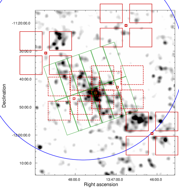
Figure 1: Layout of the observations used in this paper, superimposed to the density map of cluster members candidates (Section 8). Dashed red rectangles represent the VIMOS LR spectroscopy and solid ones are VIMOS MR masks. The large semi-circle shows the region covered by the GALEX. The tilted green mosaic represent the XMM-$Newton$ EPIC-$pn$ observations.

2.3 GALEX observations

Observations with the Galaxy Evolution Explorer (GALEX) were found in the MAST archive under program GI3_103 (PI: Hicks, see also Hicks et al. 2010 for more details). Both NUV ($\lambda_{eff}=2267$ Å) and FUV ($\lambda_{eff}=1516$ Å) bands were exposed for 9120 s. At $z\sim 0.45$ the NUV filter is similar to the rest-frame FUV filter and thus a good indicator of the unobscured star formation activity.

The limit magnitude of the NUV observations (NUV=24 AB at 3-$\sigma$) is deep enough to detect the strongest star-forming galaxies at $z\sim 0.45$, however the coverage of our field is imperfect (see Fig. 1). FUV observations are much shallower and will not be used in this work.

From the catalogues produced by the GALEX pipeline (Morrissey et al. 2007) we extracted all sources with at least 3-$\sigma$ detection significance. Objects with distances larger than 0.58 degrees from the field centre were eliminated to avoid artefacts present at the field edges.

We matched the NUV sources with our optical photometric catalogue using a search radius of 3.5″. Increasing the search radius, due to the broader GALEX PSF, does not produce more matches and contamination appears beyond 5 ″. Matched objects were also visually inspected against the $u$-band image to check the purity of the catalogue. In total, we matched 1040 objects with $0.37<z_{phot}<0.52$, our cluster galaxy selection window (see Section 3).

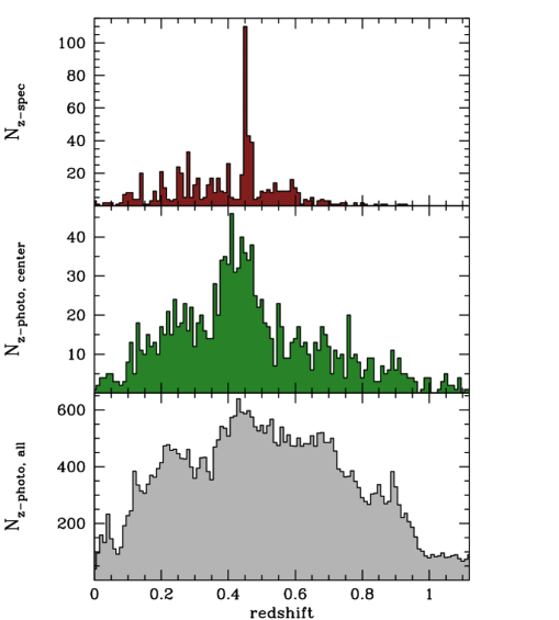
Figure 2: Upper panel: Distribution of spectroscopic redshifts from our VIMOS observations. Mid panel: Photometric redshift distribution for all galaxies in the central 10′. Lower panel: Histogram of photometric redshifts for all galaxies with $r\leq 23.5$ mag.

2.4 X-ray data

RXJ1347 has been observed with the XMM-$Newton$ X-ray telescope (ObsID:0112960101, PI: M. Turner) for 38 ks total time. Results of these observations have been reported elsewhere by Gitti & Schindler (2004) and Gitti et al. (2007).

The XMM-$Newton$ observations were focused on the central cluster and thus only a fraction of the field is covered by them (see Fig. 1). Nevertheless, they represent an opportunity to detect the X-ray emission associated to the large scale structures around RXJ1347.

We have processed the imaging using custom made software. After flare cleaning, following Zhang et al. (2004), we retained 24, 31 and 30 ks of clean time for EPIC-pn, MOS1 and MOS2, respectively. The background has been estimated using the regions of the observation free of cluster emission and point-sources. We have iterated on the definition of the background zone, as in Bielby et al. 2010, by also removing the zone of excess X-ray emission, associated with the location of the large scale structure (see Section 5.3 and Fig. 8).

In this paper we use the wavelet+PSF restoration image technique of Finoguenov et al. (2010). The objective is to report the properties of the optically selected groups (see Section 5.2), using the residual flux image after background and point source removal (including the PSF wings).

3 Cluster member selection

3.1 Photometric redshifts

The only way to establish cluster membership with high confidence is by using information from spectroscopic observations. Unfortunately, obtaining a complete sample of galaxies is very time-consuming and difficult to perform down to faint magnitudes. For that reason, in this work we use the photometric information from our multicolour imaging.

We use the code LePhare (Arnouts & Ilbert, Ilbert et al. 2006) to obtain photometric redshifts ($z_{phot}$) for all sources down to $r\sim 23.5$ mag using only the optical data. Because of the similar characteristics of our data, we have followed the procedures of Ilbert et al. (2006) to obtain photometric redshifts. In particular, we have used the same improved galaxy templates that they used for estimating redshifts for the CFHT Legacy Survey (CFHTLS). Since the GALEX data does not cover the whole field, it has not been used to obtain photometric redshifts.

We have also used spectroscopic redshifts to optimise the templates and to compensate the systematic errors in the photometry. The results from LePhare have been compared with photometric redshifts obtained using BPZ (Benítez 2000), see also Hildebrandt et al. (2009), and PHOTO-z (Bender et al. 2001, see also Brimioulle et al. 2008). The results of the three codes agree within the statistical uncertainties.

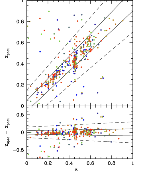
Figure 3: Comparison between photometric and the 807 spectroscopic redshifts. The solid lines mark where $|z_{spec}-z_{phot}|<0.05(1+z)$ and the dashed ones where $|z_{spec}-z_{phot}|<0.15(1+z)$. Outside of this latter limit photometric redshifts are considered catastrophic. The colour of the points indicate the best fitting template with redder colours for earlier galaxy types. The mean scatter of $z_{phot}$ is $\sigma_{z}=0.058$.

In Fig. 2 we plot the distribution of photometric redshifts for the whole field and the central 10′. A clear peak in the redshift distribution centred at $z\sim 0.45$ can be discerned. As a comparison we plot the distribution of the spectroscopic redshifts in the upper panel.

LePhare also provides information on the object type (via SED classification). This helped us to eliminate stars from the photometric catalogue below the limit of the CLASS_STAR SExtractor parameter, as stellar templates have been also included in the analysis. As galaxies dominate the number counts at faint magnitudes, we expect that the star contamination is very low in our sample.

To assess the quality of the photometric redshifts we plot in Fig. 3 a comparison between $z_{spec}$ and $z_{phot}$ as a function of $z_{spec}$. The regions marked by lines show $|z_{phot}-z_{spec}|<0.05(1+z_{spec})$ and $|z_{spec}-z_{phot}|<0.15(1+z_{spec})$ respectively. Photometric redshifts with $|z_{spec}-z_{phot}|>0.15(1+z_{spec})$ are considered catastrophic outliers.

A number of statistical tests have been proposed in the literature (e.g.  Ilbert et al. 2006; Pelló et al. 2009) to probe the quality of the photometric redshifts:

• The fraction of catastrophic outliers is defined as $|z_{spec}-z_{phot}|>0.15(1+z_{spec})$. The result is 9.12%.

• The normalised median absolute deviation $\sigma_{z,NMAD}=1.48\times$median$(|z_{spec}-z_{phot}|/(1+z))$. The result is 0.037.

• The systematic deviation between $z_{phot}$ and $z_{spec}$. $\langle\Delta(z)\rangle=\sum(z_{spec}-z_{phot})/N$, with $\Delta_{z}=|z_{spec}-z_{phot}|$. Catastrophic outliers are excluded. The result is 0.0051.

• The standard deviation of $\Delta(z)$: $\sigma_{z}=\sqrt{(\Delta(z)-\langle\Delta(z)\rangle)^{2}/(N-1)}$. The results is $\sigma_{z}=0.058$. This value represent the scatter between spectroscopic and photometric redshifts.

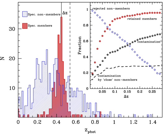
Figure 4: Photometric redshift distribution for spectroscopic confirmed members (red filled histogram) and non-members (blue hashed one). The inset shows the fraction of retained members (red circles) and rejected non-members (blue diamonds) as a function of an increasing $z_{phot}$ window threshold. The contamination due to all galaxies (black stars) is also displayed. The contamination by “close non-members” (dashed line) refers to non-cluster galaxies with $0.38<z_{spec}<0.52$, i.e.  the same redshift range we finally chose to select our cluster galaxies.

These statistical tests show that the precision of our results is comparable to those obtained with similar data (see e.g.  Ilbert et al. 2006) and the photometric redshifts display no bias compared to the spectroscopic ones. Still, they contain large uncertainties compared with spectroscopic redshifts and, therefore, any selection will introduce contamination by field interlopers and loss of cluster members.

3.2 Optimal redshift window and statistical background subtraction

As a first step, we select galaxies with photometric redshifts within an optimal range. This is done by dividing the spectroscopic sample in cluster members ($0.43<z_{spec}<0.48$) and non-members. Then we compare the fraction of retained members and rejected non-members as a function of increasing $z_{phot}$ window threshold ($\Delta z=|z_{cl}-z_{thres}|$). The contamination due to non-members is also calculated. The results of this procedure are presented in Fig. 4, where we plot the photometric redshift distribution for spectroscopic cluster members and non-members. In the inset, we plot the fraction of retained members, rejected non-members and contamination as a function of $z_{phot}$ window size.

This procedure is inspired in the selection scheme of Pelló et al. (2009). At difference of us, they used the full $z_{phot}$ probability function. In our case the probability functions calculated by Lephare are, in general, too narrow and likely not reliable, despite that their peak values are statistically accurate as shown in Fig. 3.

The optimal threshold is $\Delta z=0.07$, where $\sim$80% of the spectroscopic members are retained and a similar fraction of non-members are rejected. The contamination by non-members is $\sim$45%, however more than a half of this contamination (roughly 55%,) come from “close” non-members, i.e.  field galaxies with spectroscopic redshifts within the thresholds ($z_{spec}=0.45\pm 0.07$) which are difficult to distinguish by photo-$z$ techniques.

This final catalogue of candidate cluster members contains 5895 sources down to $r=23.5$ AB.

To correct for the contamination by field interlopers, we perform an statistical background subtraction following Pimbblet et al. (2002). For this, we use two areas of the field where the galaxy density is the lowest (see Fig. 8) to represent the field population. The total area used for this purpose is 0.285 deg².

We construct two colour-magnitude diagrams with the galaxy distribution binned in 0.1 mag in the $(g-r)$ colour and 0.25 in the $r$ magnitude. One diagram correspond to the whole cluster area and another only to the field. Both are normalised by their respective total areas.

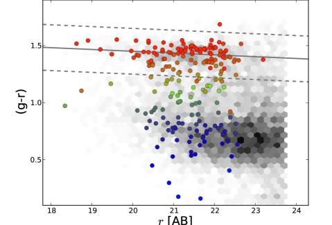
Figure 5: Observed colour-magnitude relation for spectroscopic members of RXJ1347. Each galaxy has been colour coded according to its best-fit template with redder colours for earlier types. The solid line marks the line that best describes the red-sequence fit to early type galaxies. The dashed lines are the upper and lower 3-$\sigma$ limits. The colour distribution of all photo-$z$ selected members is shown in grey scale in the background.

Afterwards, the normalised field colour-magnitude diagram is divided by the cluster one (which also contains a field signal). The result can be interpreted as the probability that a galaxy belongs to the field as a function of colour and magnitude . In other words,

$$P(\mathrm{Field})_{col,mag}=\frac{N\mathrm{(}{Field})_{col,mag}}{N\mathrm{(}{Cluster+Field})_{col,mag}}$$ (1)

Note that this procedure is also valid in the presence of incompleteness as the field and cluster signal should have a similar level of incompleteness. ’ Based on the probability map, we construct 100 Monte Carlo realisations of the parent catalogue. This is done by generating a random number between 0.0 and 1.0 for each galaxy and comparing it with its field probability according to its colour and magnitude. If this number is larger than $P(\mathrm{Field})_{col,mag}$, the galaxy is attributed to the field population and thus eliminated from the cluster catalogue. Each resulting catalogue contains between 4000 and 4400 galaxies, which should represent the true cluster population. The different quantities presented in this paper are calculated separately for each individual catalogue and then averaged. Error bars are then the standard deviation of these quantities.

3.3 The effect of the (in)accuracy of photometric redshifts

This study is based in a complete catalogue of cluster galaxies selected using moderately accurate and unbiased photometric redshifts. We have been careful in the selection of an optimal redshift bin that maximises completeness and minimises contamination. Still, the large redshift bin of $0.38<z_{phot}<0.52$ is equivalent to a transverse distance of $\sim$450 Mpc (co-moving), much larger than extent of the large scale structure around RXJ1347. Superposition of unassociated systems is therefore expected and this should be kept in mind when interpreting the results.

The use of the statistical background subtraction, with their 100 Monte Carlo generated catalogues, should correct for the mean contamination of the unassociated field. As different quantities are calculated for the individual 100 catalogues and averaged afterwards, the associated error bars should also include the uncertainty due to field contamination for a particular position of the field.

Larger than expected background fluctuations are of course difficult to assess and correct. We expect that superposition affect more strongly low density areas than high density ones like the cluster cores.

Figure 6: Colour-magnitude diagram for NUV GALEX detections with $z_{phot}$ similar to the cluster. They have been colour-coded according to the best-fit template. The sizes of the symbols are a function of the NUV magnitude. As a comparison, we plot in the background the colour-magnitude diagram for all candidate cluster galaxies from the photo-$z$ selection.

4 Galaxy colours and luminosity function

Old, passive, early type galaxies are typically located in a narrow region within the appropriate colour-magnitude diagram, usually well described by a straight line leading to the so-called the red-sequence (Baum 1959; Gladders et al. 1998).

To isolate galaxies belonging to the red-sequence, we ran LePhare on the spectroscopic catalogue keeping this time the redshift fixed. This reduces the degrees of freedom for the $\chi^{2}$ template fitting, yielding, in principle, more accurate estimates of the galaxy spectroscopic types. From the resulting catalogue we selected galaxies at $z_{spec}=0.45\pm 0.03$ with templates compatible with early types. We fitted a line to the colour-magnitude relation using a simple least-square algorithm with 3-$\sigma$ clipping in five iterations. Under these conditions this method is accurate enough for our purposes. The results can be seen in Fig. 5. The red-sequence is well approximated by the following relation: $(g-r)=-0.016\times r+1.77$ with a scatter of $\sigma=0.067$ mag.

Based on the previous fit, we define red galaxies as all galaxies with colours redder than the lower 3-$\sigma$ limit (i.e.  0.201 mag) and blue otherwise. This limit will be used to calculate the fraction of blue galaxies in the following sections. Note that this definition is identical to the original scheme proposed by Butcher & Oemler (1978).

The colour-magnitude diagram for all spectroscopic members is plotted in Fig. 5. We also plot the distribution of all photo-$z$ selected members. The bimodality of galaxy colours reported by several authors (e.g.  Baldry et al. 2006; Loh et al. 2008) is also clearly discernible here.

In Fig. 6 we plot the distribution of GALEX NUV sources in the optical colour-magnitude diagram. Practically all detected sources correspond to blue galaxies. More luminous NUV sources tend also to be brighter and bluer in the optical. As a comparison we plot also the distribution of all candidate cluster galaxies. It is evident that GALEX sources represent only a small subset the galaxy population, probably the strongest, unobscured starbursts.

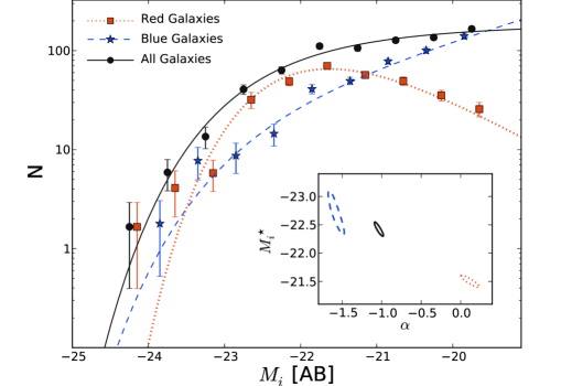
Figure 7: Rest frame $i$-bad luminosity function for all, red and blue galaxies within $2R_{200}$ (i.e.  4.6 Mpc) from the centre of RXJ1347 with the best-fit Schechter function overplotted. The inset show the 1-$\sigma$ uncertainty contours for every fit.

We also calculate the rest-frame $i$-band luminosity for all, red and blue galaxies within $2R_{200}$ (4.6 Mpc) from the centre of RXJ1347. Absolute magnitudes were obtained using the observed magnitudes and colours and applying typical k-corrections obtained with the online tool of Chilingarian et al. 2010. The frequency of galaxies per 0.5 magnitude bin was fitted with a Schechter function (Schechter 1976) of the form:

$$\phi(M)dM =0.4\ln 10\times\phi^{\star}\times 10^{-0.4(M-M^{\star})(\alpha+1)}$$ (2)

$$\times\exp\left[-10^{-0.4(M-M^{\star})}\right]dm$$

where $\phi^{\star}$ is the normalisation factor, $M^{\star}$ is the characteristic magnitude and $\alpha$ describes the faint end slope. The fitting was performed with a $\chi^{2}$-minimisation algorithm. The luminosity functions and the best fit Schechter parametrisations can be seen in Fig 7. The results for the key parameters $M^{\star}$ and $\alpha$ are the following:

• All galaxies: $M^{\star}=-22.4\pm 0.1$ mag, $\alpha=-1.04\pm 0.06$,

• Red galaxies: $M^{\star}=-21.5\pm 0.1$ mag, $\alpha=0.11\pm 0.12$,

• Blue galaxies: $M^{\star}=-22.7\pm 0.4$ mag, $\alpha=-1.58\pm 0.10$.

The values for $M^{\star}$ are in general agreement with the stacked luminosity function for $0.4<z<0.8$ clusters (see Rudnick et al. 2009 and references therein), although the luminosity function for red galaxies in RXJ1347 displays a shallower faint-end slope than the (less massive) clusters studied by the previous authors.

5 The cluster environment and the large scale structures around RXJ1347

5.1 Galaxy number density and map of the galaxy distribution

.

We use the projected galaxy number density (Dressler 1980) as a measure of the environment. For each galaxy we calculate the area of the circle of radius $r$ that encloses the 10th neighbour, so the density is defined as:

$$\Sigma_{10}=\frac{11}{\pi r_{10}^{2}}$$ (3)

This quantity was calculated for each of the 100 Montecarlo realisations of the photo-$z$ cluster catalogue (Section 3).

We preferred to use the 10th neighbour instead of the more usual fifth as projection is an issue in a photo-z selected catalogue. Using more galaxies reduces, in principle, the effects of shot noise, limiting these uncertainties.

This method can also be generalised to calculate the density for each point of a grid to produce a map of the galaxy density distribution (see Fig. 8). This procedure was called “cluster tomography” by Pelló et al. (2009) and can be considered analogous to the method used by Haines et al. (2006) to investigate the environment in the Shapley supercluster. It allows us to sample with adequate resolution the high density regions without increasing the noise in the low density ones. It can, therefore, be regarded as an adaptive smoothing method, with the advantage that it conserves the number density of galaxies at each position of the grid.

The first contour was defined at the mean density plus 1-$\sigma$ of the CFHTLS-Deep fields (Coupon et al. 2009). Taking mean and standard deviation of the four fields, we obtain a value of $\sim$11$\pm$4 galaxies/Mpc² at $z=0.45$, using the same magnitude ($r<23.5$) and photometric redshift cuts ($0.38<z_{phot}<0.52$). Note, however, that the underdense areas in our field (marked with dashed rectangles in Fig. 8). have an average density of $\sim$9$\pm$3 galaxies/Mpc², determined from statistics of the 100 Monte Carlo realisations from the parent catalogue. This makes the first contour 2-$\sigma$ over the background.

This map helps to visualise the complex dynamical situation around RXJ1347. The overdensity extends approximately in diagonal across the field $\sim$20 Mpc. Some filaments and several overdense subclumps can be seen, mainly, along this large scale structure. Some of the overdensities coincide with previously identified cluster candidates.

Besides the main cluster, two other galaxy concentrations are prominent. One towards the South-East, coincident with the cluster LCDS0825 (Gonzalez et al. 2001) and another towards the North-East without previous identification, which we will call in this paper as the NE-Clump.

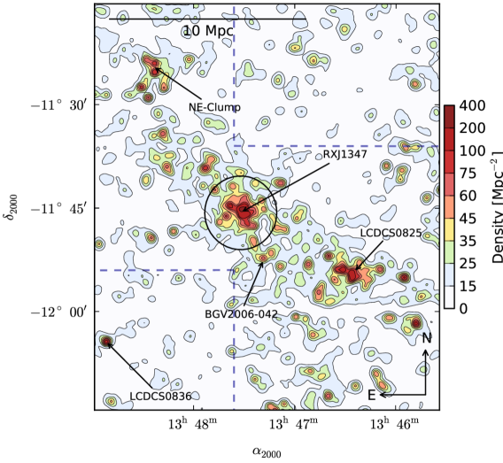
Figure 8: Map of the galaxy number density in Mpc^-2 produced by the nearest neighbour counting technique. This map is the combination of 100 individual background subtracted maps. The first contour starts at the mean of the general field at $z\sim 0.45$ plus 1-$\sigma$, obtained from CFHTLS (Coupon et al. 2009) and 2-$\sigma$ over the low density regions marked with dashed rectangles. These regions were used for the statistical background subtraction (see Section 3). Note the overdensity associated with the central cluster runs in diagonal across the field, where a complex network of filaments and subclumps can be noticed. Previously detected clusters candidates associated with overdensities at $z\sim 0.45$ have been marked, including the central cluster. The circle around RXJ1347 mark $R_{200}=2.3$ Mpc from Gitti et al. (2007).

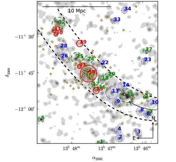
Figure 9: Distribution of the group candidates detected by the Voronoi-Delaunay algorithm over the density field. Contours are the same as in Fig. 8. The numbers are group IDs as listed in Table 2. Groups have been colour coded according their galaxy content: Blue dotted circles represent groups with $F_{blue}>0.75$, green dashed circles are groups with $0.75>F_{blue}>0.5$ and red solid circles are groups with $F_{blue}<0.5$. The large area delimited by dashed lines marks large scale structure associated with the cluster. The curved arrow indicates that distances along the LSS are measured from the lower-right corner (South-West) towards the upper-right one (North-East). Dots are galaxies with spectroscopic redshifts similar to the cluster. A zoom in of the central regions is shown in Fig. 12.

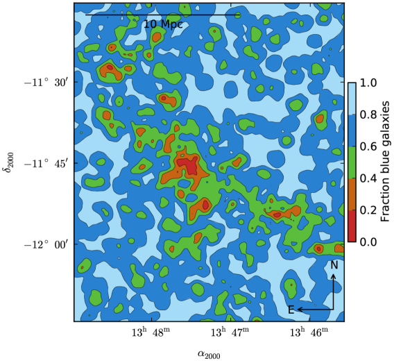
Figure 10: Map of the fraction of blue galaxies across the field. Comparing with Fig. 8, the close relation between galaxy mix and environment can be noted: Denser regions host larger fractions of red galaxies.This plot illustrates however the complexity of this relation.

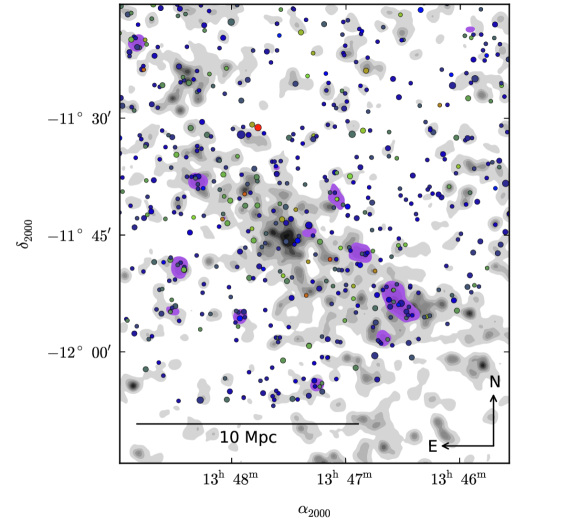
Figure 11: Distribution of GALEX NUV sources over the smoothed density field at $z=0.45$. Contours are the same as in Fig. 8. Points have been colour-coded according the best-fit spectral template based on the optical photometry. Larger symbols indicate sources with higher NUV fluxes. The purple areas indicate regions where the concentration of NUV sources exceeds 3-$\sigma$ of the field average.

5.2 Groups of galaxies

Candidate galaxy groups were detected using the Voronoi-Delaunay tessellation technique (VTT) of Ramella et al. (2001) applied to the cluster photometric catalogue. The main advantage of this method is that it does not assume any particular physical properties of groups as other techniques. This allows to select galaxy concentrations with different galaxy content and morphologies. It is also very efficient in detecting galaxy overdensities in inhomogeneous backgrounds, according to the simulations of SDSS fields by Kim et al. (2002). They also find that the efficiency of the VTT is greatly enhanced if galaxies are pre-selected in colour space, because of the improved background contrast and smaller contamination. Variations of this technique has been successfully used to produce galaxy cluster candidates catalogues either in redshift space (e.g.  Marinoni et al. 2002) or by photometric selection (e.g.  Geach et al. 2011).

The VTT of Ramella et al. (2001) is based in splitting the 2-D distribution of galaxies in independent cells, each containing only one galaxy. Galaxy groups candidates are selected from adjacent cells that satisfy a certain density threshold over the cumulative Kiang distribution (Kiang 1966) of randomly positioned points. Once a significant number of cells have been associated, the overdensity is expanded circularly to include more galaxies until the density falls under the threshold. The radius of these circles ($R_{group}$) will be interpreted as the group physical size.

We select overdensities that are significant at the 90% confidence level, i.e.  they form part of the top 90% of the density distribution. This level is higher than the one originally proposed by Ramella et al. (2001), which was 80% c.l. We reject overdensities with probabilities of being random fluctuation larger 20%, as we have already eliminated most of the contamination. We note, however, that our results are resistant to the variation these choices.

The group detection was performed in the parent catalogue but individual quantities are calculated for each of the 100 Monte Carlo realisations of the cluster catalogue. We do not claim that all of these groups are necessarily physical associations as this would require spectroscopic confirmation. They also may be unassociated to the cluster, however they allow us to probe particular environments. In total, we detect 34 group candidates.

Due to the lack of reliable mass measurements and possibly differences in their galaxy content, group candidates will be characterised by two parameters:

1. The mean density of galaxies, calculated by counting the number of galaxies within $R_{group}$. Note that this number differs from $\Sigma_{10}$ indicator introduced in the previous section.

2. The total rest-frame $i$-band luminosity, obtained from summing the individual galaxies luminosities within $R_{group}$, as a proxy of the total stellar content.

The errors of both quantities are estimated from the statistics of the 100 MonteCarlo catalogues. Comparison of different density estimates are provided in Appendix A.

In Fig. 9, we plot the distribution of the candidate groups over the density map of the field. Most of the groups are located along the large scale structure, but some are also quite isolated. The different colours indicate their different galaxy content, for red solid circles marking groups dominated by early types galaxies, green ones with an intermediate galaxy mix and blue ones, dominated by blue galaxies (see Section 8.3 for more details). Properties of the group are summarised in Table 2.

5.3 The Large Scale Structure

The overdensity associated to the cluster extends diagonally across the field for about 20 Mpc. As we also want to study the effects of the filamentary structure on galaxy evolution, we isolate galaxies belonging to this structure. This is done by modelling it by two polynomial functions that encompass most of the groups found in the large scale structure (see Fig. 9). Distance is measured from the South-West corner towards the North-East with RXJ1347 roughly at the middle.

6 Search for X-ray emission for optically identified systems

6.1 Rosat All Sky Survey

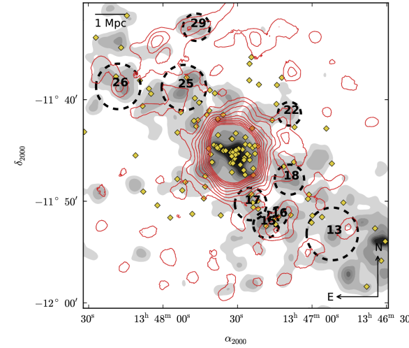
Figure 12: XMM-$Newton$ X-ray significance contours (red) superimposed to the smooth galaxy density field (gray scale). The first X-ray contour starts at 1-$\sigma$ per resolution element (32″$\times$32″) and are linearly spaced till 10-$\sigma$. The circles show the position of the optical group candidates where we performed the measurements. The numbers mark the group IDs. Small dots show the position of spectroscopic member galaxies

We performed an analysis of ROSAT All Sky Survey (RASS) data around RXJ1347 to see whether the two richer structures besides the central cluster (i.e.  LCDS0825 and the NE-Clump) have detectable X-ray emission. We measured the flux within the aperture given by the cluster detection algorithm and keeping the position fixed, i.e.  a forced detection. To measure the flux, we use two methods. 1) A wavelet technique as in Finoguenov et al. (2010), 2) the growth curve analysis of Böhringer et al. (2000).

For LCDCS0825, we find a 2-$\sigma$ detection with an upper limit for $F_{X,0.1-2.4\mathrm{\,keV}},<1.15\times 10^{-13}$ ergs s^-1 cm^-2, which implies a luminosity of $L_{X,0.1-2.4\mathrm{\,keV}}<1.2\times 10^{44}$ ergs s^-1. We take the $L_{X}-M$ relation of Leauthaud et al. (2010):

$$\frac{\langle M_{200}E(z)\rangle}{M_{0}}=A\left(\frac{\langle L_{X}E(z)^{-1}\rangle}{L_{X,0}}\right)^{\alpha}$$ (4)

where $M_{0}=10^{13.7}h_{70}^{-1}M_{\odot}$, $L_{X,0}=10^{42.7}h_{70}^{-1}$ erg s^-1, $\log_{10}(A)=0.068\pm 0.063$ and $\alpha=0.66\pm 0.14$. This sets an upper limit of $M<3.1\times 10^{14}M_{\odot}$, consistent (within the errors) with the reported weak lensing mass of Lu et al. (2010) (see more in Section 7.2). However, the low significance prevent us to set further constrains.

The North-East Clump (ID=32) has a 1$\sigma$ detection in the RASS imaging. The upper limit for its X-ray flux is: $F_{X,0.1-2.4\mathrm{\,keV}}<8.5\times 10^{14}$ ergs s^-1 cm^-2 and the luminosity $L_{X,0.1-2.4\mathrm{\,keV}}<8.2\times 10^{43}$ ergs s^-1. Using the same scaling relation, the upper mass limit is $M<1.4\times 10^{14}M_{\odot}$.

6.2 XMM-$Newton$

XMM-$Newton$ observations cover the central regions of the field (see Fig. 1), tracing part of the large scale structure associated with RXJ1347. A number of optically selected groups candidates are located in the region and we try to recover any X-ray emission from their warm-hot intergalactic medium.

Like in the previous case, we performed a forced detection, using the information from optical group detection algorithm. Point sources were removed and the background estimation (in the 0.5–2 keV range) was done using areas outside the cluster large scale structure.

In total we were able to measure the flux with over 1-$\sigma$ significance for nine groups. The properties are summarised in Table 3. The flux errors are propagated to the luminosities and mass estimates. The 20% systematic uncertainty for the mass estimates (due to the relevant scaling relation) is not listed in the errors.

The X-ray significance map is shown in Fig. 12, with contours starting at 1-$\sigma$ per resolution element (32″$\times$32″). The X-ray emission for some of the groups might the residual of the central cluster emission (groups 17, 18 and 22).

7 Clusters belonging to large scale structures around RXJ1347

Some structures in the studied field have been previously recognised. Some of them match with detected overdensities at $z\sim 0.45$ and thus are possibly associated with the RXJ1347. We have marked their position in Fig. 8. In the following we provide an individual description for some of them.

7.1 RX J1347.5-1145

This cluster was serendipitously discovered by Schindler et al. (1995) as part of the REFLEX Cluster Survey (Böhringer et al. 2001) using the ROSAT All Sky Survey (RASS). It also showed as the first strong lensing system in the REFLEX identification optical imaging.

RXJ1347 is also know as LCDCS 0829 in the Las Campanas Distant Cluster Survey (Gonzalez et al. 2001). Subsequent X-ray analysis with XMM-Newton have confirmed that it is indeed a massive structure with a X-ray luminosity in excess of $L_{X}=6.0\times 10^{45}$ erg/s in the 2–10 keV range, a temperature of $kT\sim 10$ keV and a mass estimate of $2.0\pm 0.4\times 10^{15}M_{\odot}$ within the central 1.7 Mpc (Gitti & Schindler 2004). The same authors also find a massive cooling flow with a nominal accretion rate of $\sim$1900 M_⊙/yr.

Initial discrepancies in the mass derived using X-ray, strong and weak lensing analyses, were solved by more recent studies using a combination of techniques as in Bradač et al. (2005, 2008). Furthermore, the initial low dynamical mass estimate ($\sim 4\times 10^{14}$ $M_{\odot}$) of Cohen & Kneib (2002) appears to be solved in Lu et al. (2010) by using a larger spectroscopic sample, yielding a mass well over $10^{15}$ M_⊙ in concordance with the X-ray results.

In Fig. 13 we show the redshift distribution of the cluster members from our spectroscopy. A more detailed analysis of the cluster dynamics (including mass estimates) will be presented in a forthcoming paper using the newer spectra.

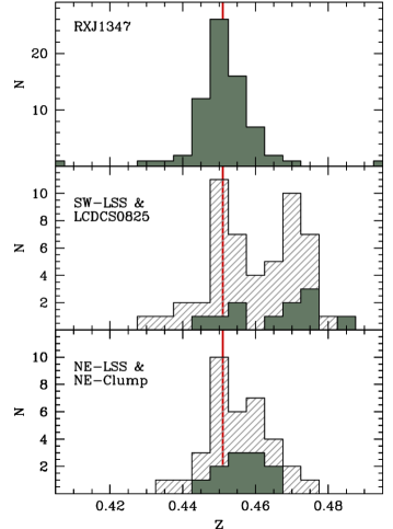
Figure 13: Spectroscopic redshift distribution for some structures in the field: Solid filled histograms show the redshift distribution for RXJ1347, LCDS0825 and the NE-Clump respectively. The hashed histograms display the redshift distributions for the associated large scale structures. The vertical line marks $z=0.45$

For the moment, we would like to add the optical mass estimate using the richness measurements following Reyes et al. (2008). The centre is taken as the peak of the X-ray emission from Schindler et al. (1997). As a first step we determine the richness $N_{200}$, which is the number of red-sequence galaxies within 1 Mpc h^-1 brighter than $0.4L^{\star}$ (i.e.  $M_{i}=-20.51$, see Fig. 7). From the statistical background subtracted catalogues, we count $N_{200}=86.9\pm 3.1$ galaxies.

Then we calculate the radius $R_{200}^{gal}=0.156\times N_{200}^{0.6}h^{-1}_{70}$ Mpc, where the galaxy density is 200 the mean of the Universe yielding a result of $R_{200}^{gal}=2.27$ Mpc. We iterate the richness estimator with this new radius obtaining a richness measure of $N_{200}=154\pm 5$ galaxies, which we finally use to estimate the mass using the formula:

$$M_{200}^{N_{200}}=(2.03\pm 0.11)\left(\frac{N_{200}}{20}\right)^{1.16\pm 0.09}\times 10^{14}M_{\odot}$$ (5)

obtaining $M_{200}^{N_{200}}=2.17^{+0.8}_{-0.6}\times 10^{15}M_{\odot}$ (random and systematics errors included), which is consistent with the estimates using other means.

We calculate the mass-to-light ratio by summing the rest-frame $i$-band luminosities of all galaxies within 1.7 Mpc. The result is $L=6.25\pm 0.2\times 10^{12}L_{\odot}$. Comparing with the reported X-ray determined mass of Gitti & Schindler (2004), we obtain a mass-to-light ratio of $M/L=320\pm 64$ $M_{\odot}/L_{\odot}$ which is typical for rich clusters (Girardi et al. 2002).

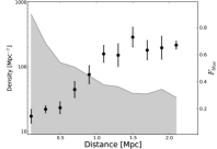
(a) RXJ1347

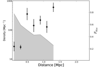
(b) LCDCS0825

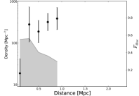
(c) NE-Clump

Figure 14: Blue fraction profiles for RXJ1347, LCDS0825 and the NE-Clump in bins of 200 kpc out to a distance of $R=1R_{200}^{gal}$. The shaded areas in the background show the density profile calculated in rings of the same size. Note the large difference in central densities and differences in the blue fraction profile.

7.2 LCDCS 0825

This structure has been previously identified as a tentative cluster by Gonzalez et al. 2001 as part of the Las Campanas Distant Cluster Survey. Lu et al. (2010) obtained a redshift $z\sim 0.47$ (RXJ1347-SW in their analysis), which we confirm. This implies a comoving distance of $\sim$62 Mpc to RXJ1347.

Although the concentration of galaxies is evident between RXJ1347 and LCDCS0825, Lu et al. (2010) were unable to confirm whether both structures are physically connected or are drifting away with cosmic expansion. Lu et al. (2010) reported a velocity dispersion of $\sigma=780\pm 100$ km s^-1 and a mass of $M_{200}=3.4^{+1.4}_{-1.1}\times 10^{14}$ M_⊙ for LCDCS0825, which would make it a relatively massive cluster. This mass is somewhat higher than the derived from the X-ray luminosity from the RASS data. However, we note that our X-ray detection has low significance and thus a large associated error (see Section 2.4). Alternatively, the mass estimates from the cluster dynamics and weak lensing might be overestimated by the presence of substructures along the line of sight. Both hypotheses are plausible given the complex optical morphology of this cluster.

The total rest-frame $i$-band luminosity for this system within 1.22 Mpc ($R_{200}$ as reported by Lu et al. 2010) is $L=2.72\pm 0.12\times 10^{12}L_{\odot}$, which implies a mass-to-light ratio of $M/L=125\pm 46$ $M_{\odot}/L_{\odot}$.

We also estimate the mass from optical traces using the Reyes et al. (2008) procedure. The centre of this object is taken from our group detection algorithm, but it is only 30″ ($\sim$170 kpc) away from the brightest cluster galaxy.

We obtain the following parameters: $N_{200}=40.7\pm 2.1$ galaxies, $R_{200}^{gal}=1.44$ Mpc, which correct the richness to $N_{200}=54\pm 4$ yielding finally a mass of $M_{200}^{N_{200}}=6.4^{+2}_{-1.9}\times 10^{14}M_{\odot}$, somewhat higher than the Lu et al. (2010) estimate from weak lensing and dynamics but well within the combined error bars.

We have at the moment few redshifts for this object, so we cannot improve the Lu et al. (2010) analysis, however we find a secondary (albeit with low significance) peak at $z\sim 0.45$ (see Fig. 13) that may indicate a complex system. Lu et al. 2010 with a larger sample do not report the lower redshift feature, although they targeted preferentially red galaxies. The redshift distribution of the associated large structure shows, however, a bimodal distribution with one peak at $z\sim 0.45$ and another at $z\sim 0.47$. It is possible that we are observing a superposition of structures in this field.

7.3 North-East clump

This object has not previously reported by studies of this field, although density and weak lensing maps by Lu et al. (2010) show a detection of this structure. We spectroscopically confirm that it is at a similar redshift with $\langle z\rangle=0.456$ and thus likely belonging to the large scale structure associated with RXJ1347. It forms, however, a sparse association without a clearly defined centre. Many bright red galaxies are associated with this structure.

The redshift distribution from the 11 available spectra for this system is quite broad, indicating that it may be still in process of assembling (see Fig. 13). Using the biweight gapper algorithm of Beers et al. (1990) (with bootstrapping), we obtain a velocity dispersion of $\sigma=1260\pm 260$ km s^-1, which would indicate a mass of $M_{200}\approx 1.9\times 10^{15}$ M_⊙ following Girardi et al. (1998) formula (corrected for the adopted cosmology). This mass estimate would make this system almost as massive as the central cluster and is surely a gross overestimate. The redshift distribution of the associated large structure is also very broad but contrary to LCDCS0825 does not show a secondary peak at $z=0.47$. Instead, it appears centred at $z\sim 0.45$ with an extended tail towards larger redshifts.

We also use the optical mass estimates, with the centre taken from our group detection algorithm, obtaining a $N_{200}=14.9\pm 01.3$ galaxies, $R_{200}^{gal}=1.12$ Mpc, a corrected richness of $N_{200}=20.5\pm 4$ and an optical mass of $M_{200}^{N_{200}}=2.1^{+1.1}_{-1}\times 10^{14}M_{\odot}$, which is likely closer to the real value and concordant with the upper limits for the X-ray luminosity (see Section 2.4).

7.3.1 LCDCS 0836

This object is a small, compact and isolated association of galaxies at $z_{phot}=0.45$. No spectroscopic redshifts are available for this object.

7.3.2 BGV2006-042

This source was detected as a candidate cluster by Barkhouse et al. (2006) in their serendipitous X-ray cluster search using Chandra archive observations. Its position coincides with a possibly infalling bright elliptical galaxy located in the middle of a filament extending towards the South-West. Five spectroscopic members are closely associated with this system (groups 15 and 16) with a median redshift of $z=0.4502$.

7.4 Blue fraction profiles for individual clusters

In Fig 14 we plot the density profile and blue fractions for the three clusters presented in the field (RXJ1347, LCDS0825 and the NE-Clump). These quantities have been calculated in radial bins of 200 kpc centred in the clusters. Error bars are shown only for the blue fraction and are obtained from the statistics of individual measurements of the 100 Monte Carlo catalogues.

The blue fraction profile for RXJ1347 is apparently smoother than for the other clusters, which seem to “jump” from low to high fractions in just a bin of radius. This may be, however, an statistical artefact given the fixed bins used and the limited number of members for the lower mass systems. In fact, the radius where LCDCS0825 and the NE-Clump reach a relatively constant value is around $R\sim 0.3R_{200}^{gal}$, which is also similar in RXJ1347. This radius is much lower than found in other studies, which is typically $R\sim 1-2R_{200}$ (e.g. Ellingson et al. 2001; Andreon et al. 2006; Verdugo et al. 2008).

First, it is important to note that we are referring to $R_{200}^{gal}$, which is typically larger than $R_{200}$ (2.9 Mpc versus 2.3 Mpc for RXJ1347). Second, we are using a photometrically selected sample, reaching fainter magnitudes than typical spectroscopic studies. As shown in Section 8, less luminous galaxies start to change their properties at higher densities than brighter ones, thus these trends are affected by this behaviour as faint galaxies dominate the number counts.

Differences on the radial trends of galaxy population for individual clusters have been, however, detected before (e.g.  Verdugo et al. 2008; Mahajan et al. 2010) and may be related to the large scale structure, dynamical properties or nature of the intracluster medium (Urquhart et al. 2010).

The density profiles for each cluster are provided to highlight the colour-density relation for these individual objects. Note the difference in the central density for each object, which also tends to be lower in the lower mass systems.

8 The cluster environment and galaxy evolution

8.1 Blue fraction vs environment

To further quantify the dependence of the galaxy mix with. environment, we plot in Fig. 15 the fraction of blue galaxies ($F_{blue}$) versus galaxy density ($\Sigma_{10}$) calculated in each 100 background subtracted catalogue. We calculated this statistic in logarithmic spaced bins and weighted it by the total number of sources in each bin. Errors bars are the 1-$\sigma$ standard deviation weighted in a similar manner.

The decline of $F_{blue}$ towards higher densities found by many authors (e.g.  Kodama et al. 2001; Pimbblet et al. 2002; Tanaka et al. 2005) is also clearly appreciable around RXJ1347. At low densities almost 90% of the galaxies are blue, whereas in the highest density bin only 10% are part of the blue population.

We then explore the dependence of this behaviour with luminosity, so we split the sample into bright ($r<22$ mag) and faint ($22\leq r<23.5$ mag) galaxies. These two populations display a somewhat distinct behaviour. The blue fraction in the bright galaxy population displays a steady decline with increasing galaxy density reaching a saturation point at $\Sigma_{10}\approx 100$ Mpc^-2. On the other hand, $F_{blue}$ for fainter galaxies starts shows a slow decline until $\Sigma_{10}\approx 40$ Mpc^-2 after which it starts to decrease at faster pace.

The fraction of blue galaxies at the lowest density bin is compatible with the values found to the field population. They are calculated using the same redshifts and magnitude cuts in the CFHTLS-Deep fields from the public available catalogues from Coupon et al. (2009) (see Section 8.2.1).

We also constructed a map of the distribution of the galaxy types traced by the fraction of blue galaxies, using a similar method as for the density map, i.e.  for each point in a grid we calculate instead the fraction of blue galaxies using the 10th nearest neighbours. As in the density map, this procedure is done for each of the 100 randomly drawn catalogues and averaged afterwards. This map is presented in Fig. 10. Comparing with the density map (Fig. 8), it is possible to visualise the relation between environment. Regions with higher fraction of red galaxies tend to located in denser environments. Despite this clear trend, the map allows to appreciate the complexities of galaxy mix with environment. There are few regions with low fraction of red galaxies without the corresponding increase in density. The opposite results also true, a few dense regions contain a high fraction of blue galaxies.

Similar maps, either of the fraction of blue galaxies or mean colour have been shown by e.g.  Haines et al. (2006) for the Shapley supercluster ($z=0.05$), Schirmer et al. (2011) for the supercluster SCL2243-0935 at $z=0.45$ and Fassbender et al. (2008) for a cluster complex at $z=0.95$. All these works have highlighted the complexities of the distribution of galaxy types against mean galaxy density over large scales.

8.2 Star formation activy around RXJ1347

We also quantify the distribution of the star-forming population by comparing the fraction of GALEX NUV sources as a function of galaxy number density. The results are presented in Fig. 16. Due to the smaller sample, we are unable to cover the same range of densities as in the case of the general blue population. The decline of the fraction of star-forming galaxies is a factor two between 10 Mpc^-2 and 80 Mpc^-2, which is similar for the blue fraction.

Comparing the number of the unobscured starbursts detected by GALEX to the general blue population, we find that this fraction is similar across the full range of densities traced here. It is also similar to to the fraction found for COSMOS field (see more in Section 8.2.1). The large error bars in the highest density bin are an indication of the very low number of star-forming galaxies found in the central regions of clusters. This results indicates that the GALEX NUV sources at our flux limits are a constant fraction of the blue population.

To test whether the properties star-forming population change with environment, we calculate the rest-frame UV luminosity function in three environments: The low density environment with $\Sigma_{10}<20$ Mpc^-2, the medium with $20\leq\Sigma_{10}<40$ Mpc^-2 and high density one with $\Sigma_{10}\geq 40$ Mpc^-2.

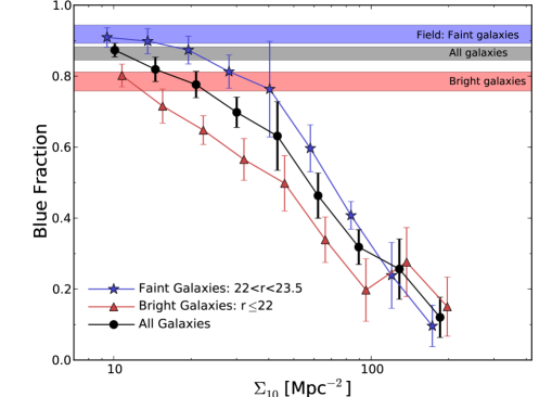
Figure 15: Fraction of blue galaxies as a function of the galaxy number density, for all galaxies (black circles), faint galaxies (blue stars) and bright ones (red triangles) as indicated in the figure. The horizontal regions mark the field fraction for the same magnitude cuts, obtained by averaging the four CFHTLS-Deep fields (Coupon et al. 2009).

Absolute magnitudes were calculated directly from the apparent NUV magnitudes without applying k-corrections. As the GALEX NUV filter at $z=0.45$ has a $\lambda_{eff}\approx 1500$ Å (similar to the rest-frame FUV filter), we expect that the introduced errors are small.

The luminosity functions are plotted in Fig. 17, together with the best-fit Schechter function (Schechter 1976, Eq. 2), obtained from a $\chi^{2}$ minimisation algorithm. The inset show the 1-$\sigma$ confidence limits. The results for the characteristic magnitude $M^{\star}_{UV}$ and the faint-end slope $\alpha$ are the following:

• Low density: $M^{\star}_{UV}$ = -19.47 $\pm$ 0.24, $\alpha$=-0.77 $\pm$ 0.29

• Medium density: $M^{\star}_{UV}$ = -19.46 $\pm$ 0.45, $\alpha$=-0.65 $\pm$ 0.50

• High density: $M^{\star}_{UV}$ = -19.33 $\pm$ 0.93, $\alpha$=-0.43 $\pm$ 1.25

The values of $M^{\star}_{UV}$ are about 1.3 mag brighter than in $z\sim 0$ clusters (e.g.  Haines et al. 2011a), but consistent with field values at $z\sim 0.5$ (Arnouts et al. (2005)). The faint-end slopes are however in our case somewhat shallower. This might be due to our relatively bright magnitude limit which does not allow us to sample adequately the faint-end of the luminosity function.

We also show in Fig. 17 the median $(g-r)$ colours for the star-forming population as a function of the environment, together with the respective 25 and 75 percentiles of the distribution. The density bins are the same as in Fig. 16. The colours of the star-forming population is very similar across all galaxy densities.

Finally, we calculate the ultraviolet spectral slope $\beta$ for NUV sources. This parameter has been shown to be sensitive to the extinction in normal star-forming galaxies (e.g.  Kong et al. 2004). We use the $u$-band and NUV magnitudes ($\lambda_{eff}\approx 1560$ and $2580$ Å at $z=0.45$ respectively) and a variation of formula of Kong et al. (2004) for local galaxies:

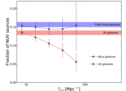
Figure 16: Fraction of detected GALEX NUV sources compared with all galaxies and only blue ones, plotted as a function of galaxy number density. The number of the strong starburst detected by GALEX decreases towards the high density regions, but they represent a constant fraction of the blue population. The field fraction obtained for the COSMOS field is shown by the horizontal regions.

$$\beta=\frac{\log(f_{NUV})-\log(f_{u})}{\log(\lambda_{NUV})-\log(\lambda_{u})}$$ (6)

where $\lambda_{NUV}$ and $\lambda_{u}$ are the respective effective wavelengths for those bands.

The median of the values as a function of galaxy density is shown in the middle in the right panel of Fig. 17, together with the 25 and 75 percentiles of the distribution. These values are typical for UV-selected star forming galaxies (Schiminovich et al. 2005) and do not differ much with the population in low redshift clusters (Haines et al. 2011b). They imply typical extinctions between $0.5<A_{UV}<2.5$ mag at $\lambda=1500$ Å for 50% of the sample with a median of $A_{UV}\sim 1.5$ mag. These values are also practically independent on environment.

A slight increase of the extinction is detected at intermediate densities (the top 75 percentile), however it is still within the expectations for the star forming population.

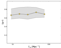
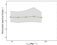
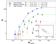
Figure 17: Properties of the NUV emitters as a function of environment. Left: The median $(g-r)$ colour. Middle: The median of the extinction sensitive ultraviolet spectral slope $\beta$. In both cases, the lower and upper lines that enclose the shaded areas represent the 25 and 75 percentiles of the distribution respectively. Right: Rest-frame UV (1450 Å) luminosity function for the GALEX sources in three different environments: The lines show the best-fit Schechter functions for three different environments: Low $\Sigma_{10}<20$ Mpc^-2, Medium with $20\leq\Sigma_{10}<40$ Mpc^-2 and high density with $\Sigma_{10}\geq 40$ Mpc^-2. The inset displays the 1-$\sigma$ uncertainty for $\alpha$ and M${}^{\star}_{UV}$ parameters.

These tests show that the star-forming population across the supercluster environment is notably homogeneous and only their relative abundance is decreasing with increasing density. This argues against a slow decline of the star formation with environment and favours a rapid change between galaxy types, as transition objects appear to be statistically insignificant from the UV perspective.

It is possible, however, that the transformation is hidden by dust as some studies suggest (e.g.  Wolf et al. 2009). In that case, the nature of the star-formation should be different than in normal galaxies, probably more centrally concentrated, making difficult to probe the UV emission due to the larger dust columns (Geach et al. 2009). However, this transition of star formation modes should also occur in short time-scales, otherwise we would detect it, either as a reddening in the colour distribution of NUV sources, as a dimming in the NUV luminosity function or as a change in the UV spectral slopes.

In Fig. 11 we show the distribution of the NUV emitters. They are sparsely with very few obvious concentrations. Some of these concentration are coincident with detected group candidates. When we construct the density map of NUV sources, using the same method described in Section 8, additional concentrations become appreciable. This is due to the different probabilities for individual galaxies assigned during the statistical background subtraction. We plot only concentrations with at least 3-$\sigma$ significance over the mean of the field. It is interesting to note that some of these concentrations are coincident with the large scale structure and candidate galaxy groups. In particular, the cluster LCDS0825 features a relatively large population of star-forming galaxies.

8.2.1 Comparison with the general field population

Our investigation is focused in the galaxy properties in the large scale structures around RXJ1347. However, the lowest density bin traced in Figs. 15 and 16 can be considered as representative of the field population as its density is lower than the mean of the CFHTLS fields. To test this and to provide proper comparison with the general field population, we use available data from current large area surveys.

In the case of Fig. 15 we used the latest public reduction of the CFHTLS-Deep fields (Coupon et al. 2009), which provides accurate photometric redshifts using a very similar methodology as our study. We use the same photometric redshifts and magnitude cuts than in our case. Since the CFHTLS-Deep fields are deeper than the data use in our investigation, their photo-$z$ are also more accurate, however we do not expect that this introduce any bias, as the effects of contamination from different redshift bins should be averaged out. In fact, it is reassuring that the blue fraction averaged for the four fields is very similar to the one measured in our lowest density bin, as can be seen in Fig. 15.

In the case of the NUV fraction comparison, we use data taken as part of the COSMOS survey centred on the CFHTLS-D2 field. Deep GALEX data has been taken over 2$\times$2 deg² on this field (PI: Schiminovich) as part of the Deep Imaging Survey (DIS) and advanced data products have been made available (e.g.  Zamojski et al. 2007). However, to make our study fully comparable, we prefer to use the data from COSMOS_00 stack, which is the shallowest stack available at MAST in this field. The total exposure time in the NUV band of 8128 s, similar to the data we are using for the cluster. We also use the catalogues produced by the GALEX pipeline. We then match the CFHTLS-D2 field (in which the COSMOS field is centred) using the same procedure as described in 2.3. NUV fractions are then calculated relative to the total population and the blue one. Like in the previous case, the general field star-forming fractions are very similar those calculated for the lowest density bin.

8.3 Galaxy properties in groups near clusters

In Fig. 9 we have plotted the distribution of the groups detected by the Voronoi-Delaunay technique (Section 5.2). Blue fractions have been calculated within an aperture given by the radius $R_{group}$ for each group for each of the individual 100 Monte Carlo catalogues. We consider “red groups”, those with $F_{blue}<0.5$; “green”, those with $0.5<F_{blue}<0.75$ and “blue”, groups with $F_{blue}>0.75$. We have marked them with the corresponding colour in Fig. 9. With some exceptions, we note that more evolved groups are located in the large scale structure and tend to be closer to larger overdensities.

To test how the evolutionary status of galaxies depends on the environmental conditions within each group, we plot in Fig. 18 the fraction of blue galaxies as a function of the mean galaxy density for each group. Despite the large scatter, a trend is observed, in which denser groups (and clusters) have lower $F_{blue}$. However, we do find few relatively dense groups (25–30 Mpc^-2 with high $F_{blue}$. Most of these groups are located at the South-West extreme of the large scale structure (see Fig. 9). A number of groups with similar mean densities contain very low $F_{blue}$, at the same level of the very massive central cluster.

Note that the fraction of blue galaxies for RXJ1347 is within the expectations from the Butcher-Oemler effect for clusters at those redshifts (e.g.  Ellingson et al. 2001; Zenteno et al. 2011).

Comparing $F_{blue}$ with the total rest-frame $i$-band luminosity for each group results in a similarly noisy correlation. More luminous systems have indeed lower $F_{blue}$, whereas the fainter ones have high fractions. In between, a high dispersion can be noted, including some relatively faint groups with very low fraction of blue galaxies.

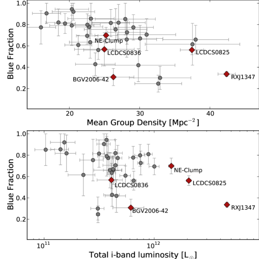
Figure 18: Fraction of blue galaxies versus the mean group density and rest-frame $i$-band luminosity for each group. Error bars are the 1-$\sigma$ standard deviations obtained from the 100 Monte Carlo catalogues. Previously detected groups and clusters are marked by red diamonds and individual identifications. Note the large scatter in galaxy content for groups of similar properties.

Although, it is difficult to assess the reality of these galaxy associations, as well as their dynamical state from photometry alone, we find these trends interesting as the evolutionary state of groups may have a stronger impact on their galaxy content than their total masses.

We finally test the overall impact of groups in colour-density relation (Fig. 15). For that we separate galaxies according to their membership. Cluster galaxies are those belonging to the three clusters in our field (namely RXJ1347, LCDS0825 and the NE-Clump). Group galaxies are those belonging to groups detected by the Voronoi technique. We include in each case all galaxies within twice the radius obtained from the group detection algorithm ($R_{group}$. This means that groups within twice the radius of the clusters are excluded to avoid duplicity. Similarly, we checked for duplicated galaxies in the composite group catalogue and eliminated them. We also created a catalogue with galaxies which do not belong to any of both categories to check the impact of the smooth density field in their properties.

Results are plotted in Fig. 19, where the fraction of blue galaxies versus galaxy density is displayed. Galaxies with no membership have a rather large blue population over a relatively large range of densities and similar to the general field. Galaxies belonging to groups display a rather modest change in $F_{blue}$ albeit with a large scatter. On the other hand, clusters exhibit a very strong change of $F_{blue}$ with density, indicating that they are very effective in transforming galaxies from one type into another. This also means that the bulk of the environmental signal in the colour-density relation (cf. Fig. 15) is likely due to these massive systems.

This does not mean that groups are not places of galaxy transformation. In fact, Fig.18 shows the large range of properties of group candidates, however it is possible that the mechanisms acting in those places are different than in clusters and not necessarily related to the galaxy density. Furthermore, it is important to note that the diversity of group properties (as well as contamination effects) may wash out some of the environmental signal.

This result is similar to those of Li et al. (2009) where a large number of photometrically selected groups around intermediate redshift clusters were analysed. They find that the environmental signal is weaker outside the virial radius of clusters. It is however in contradiction with studies at low redshift where the environmental variation of the galaxy population is similar regardless of the mass of the system (Lewis et al. 2002; Balogh et al. 2004).

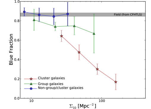
Figure 19: Blue fraction as a function of galaxy density split according to galaxy membership: Clusters, groups or none. Notice the weaker trends for non-cluster galaxies

8.4 Evolution along the large scale structure

We now test the evolution of galaxies along the large scale structure measured using an oblique area as indicated in Fig. 9. We trace the environment in this case using the position relative to the South-West corner. This may blur out the effect of small groups, but may enhance any effect purely related to the large scale structure.

We calculate the fraction of blue galaxies and GALEX NUV sources as a function of distance. The results are shown in Fig. 20. We plot in the background the mean galaxy density to appreciate its change along the LSS. The highest peaks associated with RXJ1347, LCDCS0825 and the North-East clump are evident. We can note in the plot the change of the blue fraction and how it increases when the galaxy density decreases. In particular, we note the low fraction of blue galaxies associated with the position of RXJ1347, despite the contamination of galaxies at larger radii.

The colour-density relation is somewhat broken for the South-West extreme of the large scale structure, where few dense blue dominated groups are located. The mean density increases at that point and so does the blue fraction.

Similar increases of the star formation activity with density have been only reported at high redshifts (Elbaz et al. 2007; Tran et al. 2010) or in particular environments like galaxy pairs (Ellison et al. 2008; Wong et al. 2011), but not often in groups at lower redshifts. We will wait for the results of our spectroscopic observations to make a complete assessment of the properties of these systems.

The fraction of GALEX NUV sources follows a similar trend with distance, albeit noisier due to the lower number of available sources. However, these large variations may also indicate places where the star formation is locally enhanced or suppressed depending on the local physical conditions. Unfortunately the GALEX observations do not cover the region of the previously mentioned blue dominated groups.

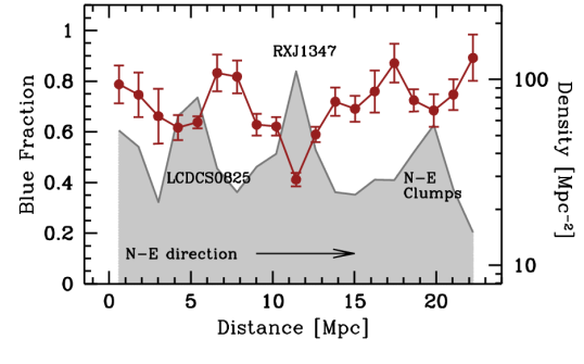
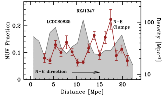
Figure 20: Fraction of blue galaxies (top) GALEX NUV sources (bottom) as a function of position within the large scale structure (red points). The origin is taken from the South-West corner (see Fig. 9). In the background, we plot in grey shade the mean galaxy density of the large scale structure. The peaks associated to main clusters are clearly discernible and marked to guide the eye. An density enhancement is also observed in the South-West extreme of the large scale structure.

9 Discussion

The study of effects of the large scale structure around clusters has been recently matter of intense research. This is motivated by the evidence that galaxy transformations start at large cluster-centric radii (Rines et al. 2005; Porter & Raychaudhury 2007; Verdugo et al. 2008; etc). As simulations in $\Lambda$CDM cosmologies predict that matter is accreted into rich clusters through filaments and infalling smaller systems (e.g.  Bond et al. 1996; Suhhonenko et al. 2011), these regions are expected to have an increase of interactions that might explain the origin of the cluster population dichotomy.

In the local universe, Mercurio et al. (2006) and Haines et al. 2006 have studied the optical properties of galaxies inhabiting the Shapley supercluster ($z=0.05$). They have shown that the environmental dependence of the global galaxy luminosity function is mostly driven by the change of the galaxy mix (colour-density relation). The luminosity function for blue galaxies is similar at all environments. Similar results were reported by Gavazzi et al. (2010) for galaxies belonging to the Coma supercluster.

In subsequent works, Haines et al. (2011a, b) have completed a census of the star formation around the Shapley supercluster by using GALEX UV and Spitzer MIR observations. They found that the respective luminosity functions for cluster star-forming galaxies do not differ significantly from comparison fields. Bai et al. (2009) and Biviano et al. (2011) have also found similar behaviour.

Using a very large catalogue of optically selected clusters, Hansen et al. (2009) have also provided evidence of the very homogeneous nature of the blue population, which depends little on system mass or clustercentric distance. This has also been confirmed by spectroscopic studies of intermediate redshift clusters. For example, Poggianti et al. (2008) and Verdugo et al. (2008) have found the mean strengths of emission lines ([OII] and H$\alpha$) for the star forming population show no dependence on environment.

Furthermore, detailed kinematical studies of spiral galaxies on distant clusters ($z=0.3-0.5$) have failed to find important differences in their velocity fields compared to the field population (Kutdemir et al. 2010). Larger samples are however needed to probe this in more detail.

In this paper, we have showed that the UV-selected star forming galaxies have similar properties at $z\sim 0.5$, regardless of their position in the large scale structure (Fig. 17). Furthermore, we provide evidence that the cluster environment plays a fundamental role in shaping their own galaxy populations and trends due to less massive galaxy systems are much weaker (Fig 19, see also Li et al. 2009).

Probably, the most viable transformation process to explain the homogeneity of the active population with environment and its rapid transformation in massive systems, is ram-pressure stripping (e.g.  Fujita 2004). This mechanism provides the necessary time-scales to make transition between galaxy types fast enough to not easily detect transition galaxy types.

Recent simulations (e.g.  Book & Benson 2010; Tecce et al. 2011) have shown that the effects of ram-pressure stripping are able to reproduce the star formation profiles in clusters out to large clustercentric distances. In Tecce et al. (2011) models, the fraction of galaxies with cold gas within $R_{200}$ depends both on cluster mass and redshift. The predicted fraction at $z=0$ is very low for clusters with masses $M_{200}>10^{14}$ M_⊙ and much higher for clusters with smaller masses. Interestingly, the relation between the blue fraction withi $R_{200}$ and cluster mass found by Hansen et al. (2009) at $z\approx 0$ remains practically flat for clusters with masses $M_{200}>10^{14}$ M_⊙ and changes rapidly below that point, indicating a change in the effectivity of the transformation processes at that mass threshold in concordance with the previous simulations.

Regarding the effects of the large scale structure in the galaxy population, we have shown that galaxy groups have a large diversity in their galaxy content (Fig 18), with little dependence on their global galaxy density or total stellar mass content. This might be signature that other effects, perhaps related to their dynamical state, alter the overall trends.

Finally, we should stress that we have found no evidence of enhanced star formation activity in the LSS as recent works have claimed (Braglia et al. 2007; Marcillac et al. 2007; Fadda et al. 2008; Porter et al. 2008). Instead we find regions with larger fractions of blue and/or star forming galaxies at moderate densities, indicating that some preprocessing is occurring in the large scale structure. Those pockets of concentrated but rather normal star formation have been also recently found around Cl 0016+16 ($z=0.55$) by Geach et al. (2011).

Tran et al. (2009), however, have found a clear increase of the star formation activity around a super group at $z\sim 0.4$. Whether such groups are abundant at intermediate redshifts is unclear. If such systems exists around RXJ1347, it might be possible that our optical-UV study are missing them due to the effects of dust attenuation. However, as it has been argued before, we should be able to detect the change of star formation modes (unobscured to obscured), if it occurs in relatively long time scales and it is caused by environmental effects.

10 Summary and prospects

We have presented a study on the large scale structures around the most luminous X-ray cluster RX J1347.5-1145. As expected from the large scale growth theory, we found that RXJ1347, one of the most massive known galaxy clusters, is embedded in a rich filamentary network, which extends for at least 20 Mpc. We have identified a number of galaxy groups in the filaments, which are likely to be accreted by the main cluster at later times. Two other massive systems are associated to the large scale structure, making RXJ1347 a good candidate for a supercluster.

We calculated the fraction of blue galaxies as a function of environment characterised by the local galaxy density. Similar to other studies we confirm the low number of blue galaxies in the high densities regions. This fraction drop from $\sim$85% in the low density environment to $\sim$10% at the highest densities in the cluster cores. This relation is also luminosity (mass) dependent.

The relation of the galaxy population with environment is also studied by using 9 ks GALEX NUV exposures, which trace the unobscured star-forming population. As a function of environment, its fraction follows closely the colour-density relation. The properties of the star-forming population is also remarkably similar at all environments. We interpretate this as evidence of a rapid transformation of galaxy types.

This is further confirmed when we analyse different environments independently. We find that the cluster environment carries most of the signal of the colour-density relation. Galaxy group candidates display, however, a large variation in their properties, signal that some transformations are also occurring in those environments, but this might not be related directly to galaxy density.

Our results are compatible with a scenario of rapid suppresion of the star-formation activity in the vicinity of clusters, likely due to specific processes. Preprocessing is also occurring in the large scale structure but its nature is apparently heterogeneous and probably depend on particular conditions.

The recently completed VIMOS campaign (30 h) over the full 1 deg² will allow us to confirm the trends studied here, via additional star formation indicators. We can identify optical AGNs and assess the properties of passive galaxies by using strong absorption lines. We would also be able to verify and investigate the properties of groups and clusters identified in this study (mostly) by photometric means.

Appendix A Comparison of densities estimates

We provide here two plots that compare estimates of the two measures of density. In the first plot (Fig. 22) two densities estimates are compared ($\Sigma_{5}$ and $\Sigma_{10}$) for all galaxies drawn from two randomly selected realizations of the 100 Monte Carlo realizations. The second plot shows the mean group density measured within the aperture $R_{group}$ versus the median density $\Sigma_{5}$ and $\Sigma_{10}$ for all galaxies within the same aperture.

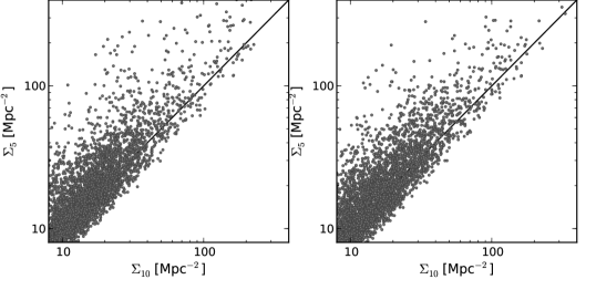
Figure 21: Comparison between $\Sigma_{10}$ and the most commonly used $\Sigma_{5}$ (10 and five neigbours respectively) for two random Monte Carlo realization of the original catalog. The line represents the one to one relation. Although both values correlate, a large scatter is appreciated.

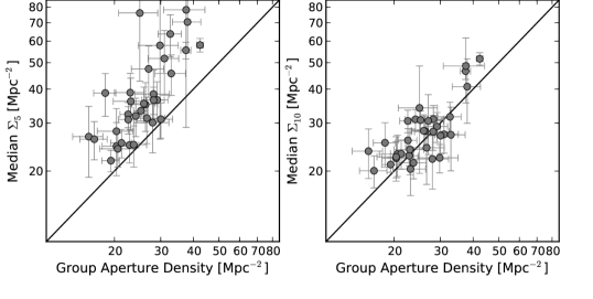
Figure 22: Comparison between the group mean density, measured within the aperture $R_{group}$, and the median $\Sigma_{5}$ and $\Sigma_{10}$ for galaxies within the same apperture. The line represents the one to one relation. Error bars are the standard deviation from the 100 Monte Carlo realizations. It is clear the $\Sigma_{5}$ overestimate the densiy for practically all groups, either due to its sensitivity to small compact association or projection effects in a photo-$z$ selected catalog.

Appendix B Tables with properties of groups around RX J1347.5-1145

In the next page, we provide the tables with properties of the optical selected groups candidates around RX J1347.5-1145. Table 2 contains the optical properties of these groups, whereas in Table 3 we provide the derived X-ray properties for those groups with detectable signal within the XMM field of view. Please see Sections 5.2 and 6 for additional details.

Table 2: List of the groups detected by the Voronoi tessellation technique. Columns: 1) Identification number, 2) and 3) Coordinates for the J2000 equinox, 4) Radius of the overdensity 5) and 6) average number of members and uncertainty, 7) and 8) Fraction of blue galaxies and associated error, 9) and 10) Total rest-frame $i$-band luminosity and error, 11) Notes for individual clusters to provide a cross identification.

(1)	(2)	(3)	(4)	(5)	(6)	(7)	(8)	(9)	(10)	(11)
ID	RA	DEC	$R_{group}$	$\langle N\rangle$	$\sigma(N)$	$\langle F_{blue}\rangle$	$\sigma(F_{blue})$	$L$	Error($L$)	Notes
	(J2000)	(J2000)	(Mpc)					($10^{11}L_{\odot}$)	($10^{11}L_{\odot}$)
1	13:47:12.2	-12:14:09	0.369	13.28	1.77	0.71	0.15	4.45	1.03
2	13:46:40.0	-12:12:14	0.493	15.6	1.83	0.94	0.06	3.69	0.72
3	13:46:08.8	-12:10:04	0.649	24.45	2.36	0.81	0.13	4.44	0.70
4	13:46:42.0	-12:08:49	0.493	15.77	2.31	0.92	0.08	1.52	0.38
5	13:48:52.0	-12:04:19	0.406	12.98	2.22	0.56	0.16	4.08	1.06	LCDS0836
6	13:45:53.2	-12:02:38	0.340	10.17	1.55	0.85	0.15	1.03	0.11
7	13:45:47.7	-12:01:37	0.356	15.19	1.87	0.65	0.13	4.25	0.79
8	13:46:03.6	-12:00:57	0.587	17.29	2.26	0.77	0.16	3.81	3.77
9	13:46:43.9	-11:57:36	0.612	34.26	3.35	0.77	0.12	4.66	4.27
10	13:45:44.4	-11:57:54	0.581	17.77	2.12	0.90	0.09	3.49	0.49
11	13:46:26.8	-11:54:28	0.987	114.7	5.06	0.56	0.05	20.6	1.02	LCDS0825
12	13:45:55.2	-11:55:04	0.273	8.84	1.58	0.61	0.19	2.27	0.62
13	13:46:51.8	-11:53:13	0.894	48.71	3.69	0.80	0.09	8.86	0.75
14	13:46:34.0	-11:50:45	0.643	29.67	2.51	0.77	0.11	6.45	0.56
15	13:47:18.4	-11:52:19	0.446	16.42	1.82	0.31	0.08	6.14	1.93	BGV2006-042
16	13:47:13.9	-11:51:32	0.321	9.15	1.38	0.66	0.17	3.96	1.14
17	13:47:24.7	-11:50:16	0.551	23.08	1.98	0.56	0.09	6.51	0.37
18	13:47:09.1	-11:47:52	0.512	23.27	2.28	0.72	0.11	7.55	0.48
19	13:47:31.6	-11:45:21	1.201	192.1	5.53	0.33	0.02	45.8	1.69	RXJ1347.5-1145
20	13:46:57.8	-11:46:08	0.435	17.93	1.93	0.66	0.12	4.24	0.24
21	13:47:47.0	-11:42:21	0.309	9.88	1.31	0.30	0.11	3.08	0.42
22	13:47:09.1	-11:41:24	0.400	13.6	1.91	0.81	0.17	1.59	0.34
23	13:45:56.8	-11:40:12	0.466	15.8	2.25	0.85	0.14	1.41	0.26
24	13:47:33.6	-11:39:57	0.676	30.59	2.75	0.60	0.09	5.48	0.61
25	13:47:51.6	-11:38:49	0.773	42.41	2.88	0.69	0.07	10.0	1.06
26	13:48:18.0	-11:38:42	0.773	42.47	3.46	0.79	0.10	7.44	0.79
27	13:45:54.9	-11:35:56	0.377	10.29	1.33	0.63	0.15	4.11	0.35
28	13:48:18.9	-11:34:30	0.529	22.78	2.33	0.81	0.13	3.15	0.39
29	13:47:46.5	-11:32:52	0.464	16.08	1.91	0.42	0.11	4.15	0.68
30	13:48:26.8	-11:29:02	0.280	7.35	1.28	0.41	0.15	4.54	0.95
31	13:48:30.0	-11:27:25	0.302	9.41	0.96	0.24	0.08	3.09	0.12
32	13:48:22.5	-11:24:39	0.925	67.87	4.25	0.69	0.07	14.3	0.79	NE-Clump
33	13:46:48.9	-11:23:34	0.379	12.04	2.02	0.75	0.19	2.78	0.67
34	13:46:30.9	-11:19:08	0.427	11.68	1.80	0.79	0.18	3.71	0.65

Table 3: X-ray fluxes and derived parameters for optically detected groups in the area covered by XMM-$Newton$ observations. Columns: 1) Identification numbers (same as in Table 2), 2) and 3) Coordinates, 4) Measured X-ray flux and error, 5) X-ray luminosity, 6) Total mass within the 7) the $R_{200}$ radius, 8) Flux significance.

(1)	(2)	(3)	(4)	(5)	(6)	(7)	(8)
ID	RA	DEC	$F_{X}$ (0.5-2 keV)	$L_{X}$	$M_{200}$	$R_{200}$	$\sigma(F_{X})$
	(J2000)	(J2000)	($10^{-15}$ erg s-1 cm-2)	($10^{42}$ erg s-1)	($10^{13}M_{\odot}$ )	(Mpc)
13	13:46:51.8	-11:53:13	$2.77\pm 1.66$	$2.83\pm 2.08$	$3.22\pm 1.12$	0.57	1.67
15	13:47:18.4	-11:52:19	$3.65\pm 1.57$	$3.71\pm 1.96$	$3.83\pm 0.98$	0.60	2.32
16	13:47:13.9	-11:51:32	$1.12\pm 0.79$	$1.21\pm 1.04$	$1.87\pm 0.75$	0.47	1.42
17	13:47:24.7	-11:50:16	$3.26\pm 1.26$	$3.32\pm 1.57$	$3.57\pm 0.82$	0.59	2.59
18	13:47:09.1	-11:47:52	$2.14\pm 0.94$	$2.20\pm 1.18$	$2.74\pm 0.71$	0.54	2.29
22	13:47:09.1	-11:41:24	$1.13\pm 0.73$	$1.22\pm 0.96$	$1.87\pm 0.70$	0.47	1.55
25	13:47:51.6	-11:38:49	$1.80\pm 1.34$	$1.87\pm 1.71$	$2.47\pm 1.05$	0.52	1.34
26	13:48:18.0	-11:38:42	$5.72\pm 1.77$	$5.77\pm 2.19$	$5.08\pm 0.95$	0.66	3.24
29	13:47:46.5	-11:32:52	$2.53\pm 1.51$	$2.59\pm 1.90$	$3.04\pm 1.06$	0.56	1.68

References

- Andreon et al. (2006) Andreon S., Quintana H., Tajer M., Galaz G., Surdej J., 2006, MNRAS, 365, 915
- Arnouts et al. (2005) Arnouts S., Schiminovich D., Ilbert O., Tresse L., Milliard B., Treyer M., et al. 2005, ApJ, 619, L43
- Bai et al. (2009) Bai L., Rieke G. H., Rieke M. J., Christlein D., Zabludoff A. I., 2009, ApJ, 693, 1840
- Baldry et al. (2006) Baldry I. K., Balogh M. L., Bower R. G., Glazebrook K., et al. 2006, MNRAS, 373, 469
- Balogh et al. (2004) Balogh M., Eke V., Miller C., Lewis I., Bower R., et al. 2004, MNRAS, 348, 1355
- Balogh et al. (1999) Balogh M. L., Morris S. L., Yee H. K. C., Carlberg R. G., Ellingson E., 1999, ApJ, 527, 54
- Barkhouse et al. (2006) Barkhouse W. A., Green P. J., Vikhlinin A., Kim D., Perley D., et al. 2006, ApJ, 645, 955
- Bauer et al. (2011) Bauer A. E., Grützbauch R., Jørgensen I., Varela J., Bergmann M., 2011, MNRAS, 411, 2009
- Baum (1959) Baum W. A., 1959, PASP, 71, 106
- Beers et al. (1990) Beers T. C., Flynn K., Gebhardt K., 1990, AJ, 100, 32
- Bender et al. (2001) Bender R., Appenzeller I., Böhm A., et al. 2001, pp 96–+
- Benítez (2000) Benítez N., 2000, ApJ, 536, 571
- Bertin & Arnouts (1996) Bertin E., Arnouts S., 1996, A&AS, 117, 393
- Bielby et al. (2010) Bielby R. M., Finoguenov A., Tanaka M., McCracken H. J., Daddi E., Hudelot P., et al. 2010, A&A, 523, A66+
- Biviano et al. (2011) Biviano A., Fadda D., Durret F., Edwards L. O. V., Marleau F., 2011, A&A, 532, A77
- Böhringer et al. (2004) Böhringer H., Schuecker P., Guzzo L., Collins C. A., Voges W., et al. 2004, A&A, 425, 367
- Böhringer et al. (2001) Böhringer H., Schuecker P., Guzzo L., Collins C. A., Voges W., Schindler S., et al. 2001, A&A, 369, 826
- Böhringer et al. (2000) Böhringer H., Voges W., Huchra J. P., McLean B., Giacconi R., Rosati P., et al. 2000, ApJS, 129, 435
- Bond et al. (1996) Bond J. R., Kofman L., Pogosyan D., 1996, Nature, 380, 603
- Book & Benson (2010) Book L. G., Benson A. J., 2010, ApJ, 716, 810
- Bradač et al. (2005) Bradač M., Erben T., Schneider P., Hildebrandt H., Lombardi M., Schirmer M., et al. 2005, A&A, 437, 49
- Bradač et al. (2008) Bradač M., Schrabback T., Erben T., McCourt M., Million E., Mantz A., Allen et al. 2008, ApJ, 681, 187
- Braglia et al. (2007) Braglia F., Pierini D., Böhringer H., 2007, A&A, 470, 425
- Braglia et al. (2009) Braglia F. G., Pierini D., Biviano A., Böhringer H., 2009, A&A, 500, 947
- Brimioulle et al. (2008) Brimioulle F., Lerchster M., Seitz S., Bender R., Snigula J., 2008, ArXiv e-prints
- Butcher & Oemler (1978) Butcher H., Oemler Jr. A., 1978, ApJ, 226, 559
- Chilingarian et al. (2010) Chilingarian I. V., Melchior A.-L., Zolotukhin I. Y., 2010, MNRAS, 405, 1409
- Christlein & Zabludoff (2005) Christlein D., Zabludoff A. I., 2005, ApJ, 621, 201
- Cohen & Kneib (2002) Cohen J. G., Kneib J.-P., 2002, ApJ, 573, 524
- Coupon et al. (2009) Coupon J., Ilbert O., Kilbinger M., McCracken H. J., Mellier Y., Arnouts S., et al. 2009, A&A, 500, 981
- Dressler (1980) Dressler A., 1980, ApJ, 236, 351
- Dressler et al. (1985) Dressler A., Thompson I. B., Shectman S. A., 1985, ApJ, 288, 481
- Elbaz et al. (2007) Elbaz D., Daddi E., Le Borgne D., Dickinson M., Alexander D. M., Chary R.-R., et al. 2007, A&A, 468, 33
- Ellingson et al. (2001) Ellingson E., Lin H., Yee H. K. C., Carlberg R. G., 2001, ApJ, 547, 609
- Ellison et al. (2008) Ellison S. L., Patton D. R., Simard L., McConnachie A. W., 2008, AJ, 135, 1877
- Erben et al. (2009) Erben T., Hildebrandt H., Lerchster M., Hudelot P., Benjamin J., et al. 2009, A&A, 493, 1197
- Ettori et al. (2001) Ettori S., Allen S. W., Fabian A. C., 2001, MNRAS, 322, 187
- Fadda et al. (2008) Fadda D., Biviano A., Marleau F. R., Storrie-Lombardi L. J., Durret F., 2008, ApJ, 672, L9
- Fassbender et al. (2008) Fassbender R., Böhringer H., Lamer G., Mullis C. R., Rosati P., et al. 2008, A&A, 481, L73
- Finn et al. (2010) Finn R. A., Desai V., Rudnick G., Poggianti B., Bell E. F., Hinz J., et al. 2010, ApJ, 720, 87
- Finoguenov et al. (2010) Finoguenov A., Watson M. G., Tanaka M., Simpson C., et al. 2010, MNRAS, 403, 2063
- Fujita (2004) Fujita Y., 2004, PASJ, 56, 29
- Gallazzi et al. (2009) Gallazzi A., Bell E. F., Wolf C., Gray M. E., Papovich C., Barden M., Peng C. Y., et al. 2009, ApJ, 690, 1883
- Garilli et al. (2010) Garilli B., Fumana M., Franzetti P., Paioro L., Scodeggio M., Le Fèvre O., et al. 2010, PASP, 122, 827
- Gavazzi et al. (2010) Gavazzi G., Fumagalli M., Cucciati O., Boselli A., 2010, A&A, 517, A73+
- Geach et al. (2011) Geach J. E., Ellis R. S., Smail I., Rawle T. D., Moran S. M., 2011, MNRAS, 413, 177
- Geach et al. (2011) Geach J. E., Murphy D. N. A., Bower R. G., 2011, MNRAS, 413, 3059
- Geach et al. (2009) Geach J. E., Smail I., Moran S. M., Treu T., Ellis R. S., 2009, ApJ, 691, 783
- Girardi et al. (1998) Girardi M., Giuricin G., Mardirossian F., Mezzetti M., Boschin W., 1998, ApJ, 505, 74
- Girardi et al. (2002) Girardi M., Manzato P., Mezzetti M., Giuricin G., Limboz F., 2002, ApJ, 569, 720
- Gitti et al. (2007) Gitti M., Ferrari C., Domainko W., Feretti L., Schindler S., 2007, A&A, 470, L25
- Gitti et al. (2007) Gitti M., Piffaretti R., Schindler S., 2007, A&A, 472, 383
- Gitti & Schindler (2004) Gitti M., Schindler S., 2004, A&A, 427, L9
- Gladders et al. (1998) Gladders M. D., Lopez-Cruz O., Yee H. K. C., Kodama T., 1998, ApJ, 501, 571
- Gonzalez et al. (2001) Gonzalez A. H., Zaritsky D., Dalcanton J. J., Nelson A., 2001, ApJS, 137, 117
- Haines et al. (2011a) Haines C. P., Busarello G., Merluzzi P., Smith R. J., Raychaudhury S., et al. 2011a, MNRAS, 412, 127
- Haines et al. (2011b) Haines C. P., Busarello G., Merluzzi P., Smith R. J., Raychaudhury S., et al. 2011b, MNRAS, 412, 145
- Haines et al. (2006) Haines C. P., La Barbera F., Mercurio A., Merluzzi P., Busarello G., 2006, ApJ, 647, L21
- Haines et al. (2006) Haines C. P., Merluzzi P., Mercurio A., Gargiulo A., Krusanova N., Busarello G., et al. 2006, MNRAS, 371, 55
- Haines et al. (2009) Haines C. P., Smith G. P., Egami E., Ellis R. S., Moran S. M., Sanderson A. J. R., et al. 2009, ApJ, 704, 126
- Haines et al. (2009) Haines C. P., Smith G. P., Egami E., Okabe N., Takada M., Ellis R. S., et al. 2009, MNRAS, 396, 1297
- Halkola et al. (2008) Halkola A., Hildebrandt H., Schrabback T., Lombardi M., Bradač M., Erben T., et al. 2008, A&A, 481, 65
- Hansen et al. (2009) Hansen S. M., Sheldon E. S., Wechsler R. H., Koester B. P., 2009, ApJ, 699, 1333
- Hicks et al. (2010) Hicks A. K., Mushotzky R., Donahue M., 2010, ApJ, 719, 1844
- Hildebrandt et al. (2009) Hildebrandt H., Pielorz J., Erben T., van Waerbeke L., Simon P., Capak P., 2009, A&A, 498, 725
- Ilbert et al. (2006) Ilbert O., Arnouts S., McCracken H. J., Bolzonella M., Bertin E., Le Fèvre O., et al. 2006, A&A, 457, 841
- Kiang (1966) Kiang T., 1966, ZAp, 64, 433
- Kim et al. (2002) Kim R. S. J., Kepner J. V., Postman M., Strauss M. A., Bahcall N. A., Gunn J. E., et al. 2002, AJ, 123, 20
- Kitayama et al. (2004) Kitayama T., Komatsu E., Ota N., Kuwabara T., Suto Y., Yoshikawa K., Hattori M., Matsuo H., 2004, PASJ, 56, 17
- Kodama et al. (2001) Kodama T., Smail I., Nakata F., Okamura S., Bower R. G., 2001, ApJ, 562, L9
- Komatsu et al. (2001) Komatsu E., Matsuo H., Kitayama T., Hattori M., Kawabe R., et al. 2001, PASJ, 53, 57
- Kong et al. (2004) Kong X., Charlot S., Brinchmann J., Fall S. M., 2004, MNRAS, 349, 769
- Koyama et al. (2008) Koyama Y., Kodama T., Shimasaku K., Okamura S., Tanaka M., Lee H. M., et al. 2008, MNRAS, 391, 1758
- Kutdemir et al. (2010) Kutdemir E., Ziegler B. L., Peletier R. F., Da Rocha C., Böhm A., Verdugo M., 2010, A&A, 520, A109+
- Leauthaud et al. (2010) Leauthaud A., Finoguenov A., Kneib J., Taylor J. E., Massey R., Rhodes J., et al. 2010, ApJ, 709, 97
- Lewis et al. (2002) Lewis I., Balogh M., De Propris R., Couch W., Bower R., Offer A., et al. 2002, MNRAS, 334, 673
- Li et al. (2009) Li I. H., Yee H. K. C., Ellingson E., 2009, ApJ, 698, 83
- Loh et al. (2008) Loh Y.-S., Ellingson E., Yee H. K. C., Gilbank D. G., Gladders M. D., Barrientos L. F., 2008, ApJ, 680, 214
- Lu et al. (2010) Lu T., Gilbank D. G., Balogh M. L., Milkeraitis M., Hoekstra H., van Waerbeke L., et al. 2010, MNRAS, 403, 1787
- Mahajan et al. (2010) Mahajan S., Haines C. P., Raychaudhury S., 2010, MNRAS, 404, 1745
- Marcillac et al. (2007) Marcillac D., Rigby J. R., Rieke G. H., Kelly D. M., 2007, ApJ, 654, 825
- Marinoni et al. (2002) Marinoni C., Davis M., Newman J. A., Coil A. L., 2002, ApJ, 580, 122
- Mason et al. (2010) Mason B. S., Dicker S. R., Korngut P. M., et al. 2010, ApJ, 716, 739
- Medezinski et al. (2010) Medezinski E., Broadhurst T., Umetsu K., Oguri M., Rephaeli Y., Benítez N., 2010, MNRAS, 405, 257
- Mercurio et al. (2006) Mercurio A., Merluzzi P., Haines C. P., Gargiulo A., Krusanova N., Busarello G., et al. 2006, MNRAS, 368, 109
- Moran et al. (2007) Moran S. M., Ellis R. S., Treu T., Smith G. P., Rich R. M., Smail I., 2007, ApJ, 671, 1503
- Morrissey et al. (2007) Morrissey P., Conrow T., Barlow T. A., Small T., et al. 2007, ApJS, 173, 682
- Ota et al. (2008) Ota N., Murase K., Kitayama T., Komatsu E., Hattori M., et al. 2008, A&A, 491, 363
- Pelló et al. (2009) Pelló R., Rudnick G., De Lucia G., Simard L., Clowe D. I., Jablonka P., et al. 2009, A&A, 508, 1173
- Pickles (1998) Pickles A. J., 1998, PASP, 110, 863
- Pimbblet et al. (2002) Pimbblet K. A., Smail I., Kodama T., Couch W. J., Edge A. C., Zabludoff A. I., O’Hely E., 2002, MNRAS, 331, 333
- Poggianti et al. (2008) Poggianti B. M., Desai V., Finn R., Bamford S., De Lucia G., et al. 2008, ApJ, 684, 888
- Popesso et al. (2007) Popesso P., Biviano A., Romaniello M., Böhringer H., 2007, A&A, 461, 411
- Porter & Raychaudhury (2007) Porter S. C., Raychaudhury S., 2007, MNRAS, 375, 1409
- Porter et al. (2008) Porter S. C., Raychaudhury S., Pimbblet K. A., Drinkwater M. J., 2008, MNRAS, 388, 1152
- Ramella et al. (2001) Ramella M., Boschin W., Fadda D., Nonino M., 2001, A&A, 368, 776
- Reyes et al. (2008) Reyes R., Mandelbaum R., Hirata C., Bahcall N., Seljak U., 2008, MNRAS, 390, 1157
- Rines et al. (2005) Rines K., Geller M. J., Kurtz M. J., Diaferio A., 2005, AJ, 130, 1482
- Rudnick et al. (2009) Rudnick G., von der Linden A., Pelló R., Aragón-Salamanca A. ., et al. 2009, ApJ, 700, 1559
- Saintonge et al. (2008) Saintonge A., Tran K., Holden B. P., 2008, ApJ, 685, L113
- Schechter (1976) Schechter P., 1976, ApJ, 203, 297
- Schiminovich et al. (2005) Schiminovich D., Ilbert O., Arnouts S., Milliard B., Tresse L., Le Fèvre O., et al. 2005, ApJ, 619, L47
- Schindler et al. (1995) Schindler S., Guzzo L., Ebeling H., Boehringer H., Chincarini G., Collins C. A., et al. 1995, A&A, 299, L9+
- Schindler et al. (1997) Schindler S., Hattori M., Neumann D. M., Boehringer H., 1997, A&A, 317, 646
- Schirmer et al. (2011) Schirmer M., Hildebrandt H., Kuijken K., Erben T., 2011, A&A, 532, A57+
- Schlegel et al. (1998) Schlegel D. J., Finkbeiner D. P., Davis M., 1998, ApJ, 500, 525
- Scodeggio et al. (2005) Scodeggio M., Franzetti P., Garilli B., Zanichelli A., Paltani S., et al. 2005, PASP, 117, 1284
- Suhhonenko et al. (2011) Suhhonenko I., Einasto J., Liivamägi L. J., Saar E., Einasto M., et al. 2011, A&A, 531, A149+
- Tanaka et al. (2009) Tanaka M., Finoguenov A., Kodama T., Koyama Y., Maughan B., Nakata F., 2009, A&A, 505, L9
- Tanaka et al. (2007) Tanaka M., Hoshi T., Kodama T., Kashikawa N., 2007, MNRAS, 379, 1546
- Tanaka et al. (2005) Tanaka M., Kodama T., Arimoto N., Okamura S., Umetsu K., et al. 2005, MNRAS, 362, 268
- Tecce et al. (2011) Tecce T. E., Cora S. A., Tissera P. B., 2011, MNRAS, 416, 3170
- Tran et al. (2010) Tran K., Papovich C., Saintonge A., et al. 2010, ApJ, 719, L126
- Tran et al. (2009) Tran K., Saintonge A., Moustakas J., Bai L., Gonzalez A. H., et al. 2009, ApJ, 705, 809
- Urquhart et al. (2010) Urquhart S. A., Willis J. P., Hoekstra H., Pierre M., 2010, MNRAS, 406, 368
- Verdugo et al. (2008) Verdugo M., Ziegler B. L., Gerken B., 2008, A&A, 486, 9
- von der Linden et al. (2010) von der Linden A., Wild V., Kauffmann G., White S. D. M., Weinmann S., 2010, MNRAS, 404, 1231
- Wolf et al. (2009) Wolf C., Aragón-Salamanca A., Balogh M., Barden M., Bell E. F., Gray M. E. ., et al. 2009, MNRAS, 393, 1302
- Wong et al. (2011) Wong K. C., Blanton M. R., Burles S. M., Coil A. L., Cool R. J., et al. 2011, ApJ, 728, 119
- Yee et al. (1996) Yee H. K. C., Ellingson E., Carlberg R. G., 1996, ApJS, 102, 269
- Zamojski et al. (2007) Zamojski M. A., Schiminovich D., Rich R. M., Mobasher B., Koekemoer A. M., et al. 2007, ApJS, 172, 468
- Zenteno et al. (2011) Zenteno A., Song J., Desai S., Armstrong R., Mohr J. J., Ngeow C.-C., Barkhouse W. A., et al. 2011, ApJ, 734, 3
- Zhang et al. (2006) Zhang Y., Böhringer H., Finoguenov A., Ikebe Y., Matsushita K., et al. 2006, A&A, 456, 55
- Zhang et al. (2004) Zhang Y., Finoguenov A., Böhringer H., Ikebe Y., Matsushita K., Schuecker P., 2004, A&A, 413, 49