Going off grid: Computationally efficient inference for log-Gaussian Cox processes

Abstract

This paper introduces a new method for performing computational inference on log-Gaussian Cox processes. The likelihood is approximated directly by making novel use of a continuously specified Gaussian random field. We show that for sufficiently smooth Gaussian random field prior distributions, the approximation can converge with arbitrarily high order, while an approximation based on a counting process on a partition of the domain only achieves first-order convergence. The given results improve on the general theory of convergence of the stochastic partial differential equation models, introduced by Lindgren et al. (2011). The new method is demonstrated on a standard point pattern data set and two interesting extensions to the classical log-Gaussian Cox process framework are discussed. The first extension considers variable sampling effort throughout the observation window and implements the method of Chakraborty et al. (2011). The second extension constructs a log-Gaussian Cox process on the world’s oceans. The analysis is performed using integrated nested Laplace approximation for fast approximate inference.

1 Introduction

Data consisting of sets of locations at which some objects are present are common in biology, ecology and economics. The appropriate statistical models for this type of data are spatial point process models, which have been extensively studied by statisticians and probabilists (Møller & Waagepetersen, 2004; Illian et al., 2008) but are less commonly used by the scientists producing the data sets. Point process models are often hard to fit, so scientists often resort to using inappropriate methods. (Chakraborty et al., 2011) discuss this in the context of presence-only datasets, and outline various ad hoc approaches used by ecologistsThere is an interesting discussion of this in the context of presence only data sets (Chakraborty et al., 2011), which outlines a number of ad hoc approaches taken by the ecological community.

Many real data sets do not have the simple structure usually considered in the classical statistical literature, i.e., that of a simple point pattern that has been observed everywhere within a simple, often rectangular, plot. For instance, in real data sets the observation process is often not straightforward due to practical limitations, or the observation window is complex. This includes data sets mapping the locations of bird species, for which very little data have been collected in the Himalayas for obvious reasons. Therefore, on top of sampling issues such as incompletely observed point patterns, positional errors, etc., this data set has a large hole where it is believed that birds reside, but it is impractical to look for them. Very different, but similarly complex, data deal with freak waves in the oceans. Even if we ignore temporal aspects, or the uncertainty in the observed locations, this data set remains complicated, as the observation window covers most of a sphere and has a very complicated boundary. Motivated by data sets of this nature, this paper proposes an easy to use, computationally efficient method for performing inference on spatial point process models that is sufficiently flexible to handle these and other data structures.

In this paper we focus on log-Gaussian Cox processes, a class of flexible models that is particularly useful in the context of modelling aggregation relative to some underlying unobserved environmental field (Møller et al., 1998; Illian et al., 2012). However, standard methods for fitting Cox processes are computationally expensive and the Markov chain Monte Carlo methods that are commonly used are difficult to tune for this problem. Recently, Illian et al. (2012) developed a fast, flexible framework for fitting log-Gaussian Cox processes using integrated nested Laplace approximation (Rue et al., 2009). They construct a Poisson approximation to the true log-Gaussian Cox process likelihood to perform inference on a regular lattice over the observation window, counting the number of points in each cell. If the lattice is fine enough and the latent Gaussian field is appropriately discretised, this approximation is quite good (Waagepetersen, 2004), but it can be computationally wasteful, especially when the process intensity is high or the observation window is large or oddly shaped. New results on the strong convergence of the lattice approximation, provided in the Appendix, show that the rate of convergence on a $p\times p$ lattice is fundamentally limited to $\mathcal{O}(p^{-1})$ by the counting approximation.

In the Appendix, we provide detailed results on the convergence of the approximations proposed in this paper. In particular, we show that, for a Gaussian random field with fixed parameters, the posterior distributions generated using the proposed method will converge strongly to the true posterior distribution. Furthermore, it is shown that these posterior distributions can converge with arbitrarily high order and the convergence is limited only by the smoothness of the random field. In this paper, we place particular emphasis on the combination of this method with the flexible stochastic partial differential equation models of Lindgren et al. (2011) and we significantly improve the existing convergence theory for these models. In particular, we show that the approximate posterior distributions converge weakly and the error when computing a posterior functional is almost $\mathcal{O}(h^{-1})$.

The first of our aims is to re-examine the standard methodology for Bayesian inference on log-Gaussian Cox processes and to propose an approach that is much more computationally efficient based on continuously specified finite-dimensional Gaussian random fields. The key characteristic of our approach is that the specification of the Gaussian random field is completely separated from the approximation of the likelihood, leading to far greater flexibility. The second aim is to demonstrate that this approach can be handled within the general approximation framework of Rue et al. (2009), by modelling the Gaussian random field through a stochastic partial differential equation (Lindgren et al., 2011). This provides a unified modelling structure. An associated R-package makes our methods that accessible to scientists.

2 Log-Gaussian Cox processes

Consider a bounded region $\Omega\subset\mathbb{R}^{2}$. A simple point process model is the inhomogeneous Poisson process, in which the number of points within a region $D\subset\Omega$ is Poisson distributed with mean $\Lambda(D)=\int_{D}\lambda(s)\,ds$, where $\lambda(s)$ is the intensity surface of the point process. Given the intensity surface and a point pattern $Y,$ the likelihood of an inhomogeneous Poisson process is

$$\pi({Y}\mid\lambda)=\exp\left\{|\Omega|-\int_{\Omega}\lambda(s)\,ds\right\}\prod_{s_{i}\in Y}\lambda(s_{i}).$$ (1)

This likelihood is analytically intractable, as it requires the integral of the intensity function, which typically cannot be calculated explicitly. This integral can, however, be computed numerically using standard methods.

Treating the intensity surface as a realisation of a random field $\lambda(s)$ yields a particularly flexible class of point processes known as Cox or doubly stochastic Poisson processes (Møller & Waagepetersen, 2004). These are typically used to model aggregation in point patterns resulting from observed or unobserved environmental variation. In this paper we consider log-Gaussian Cox processes, where the intensity surface is modelled as $\log\lambda(s)={Z}(s)$, and ${Z}(s)$ is a Gaussian random field. Conditional on a realisation of ${Z}(s)$, a log-Gaussian Cox process is an inhomogeneous Poisson process. The likelihood for such a process is of the form (1), where the integral is further complicated by the stochastic nature of $\lambda(s)$, and methods for approximating (1) are the focus of the next two sections. Log-Gaussian Cox processes fit naturally within the Bayesian hierarchical modelling framework and are latent Gaussian models. They may be fitted using the integrated nested Laplace approximation approach of Rue et al. (2009), allowing us to construct models that include covariates, marks and non-standard observation processes while still allowing computationally efficient inference (Illian et al., 2012). Therefore, approximating the likelihood in (1) constitutes a basic calculation for practical problems such as those discussed in Section 7.

3 Computation on fine lattices is wasteful

A common method for performing inference with log-Gaussian Cox processes is to take the observation window $\Omega$, construct a fine regular lattice over it, and then consider the number of points $N_{ij}$ observed in each cell $s_{ij}$ of the lattice (Møller et al., 1998; Illian et al., 2012). It is a simple consequence of the definition of a log-Gaussian Cox process that the $N_{ij}$ may be considered as independent Poisson random variables, that is $N_{ij}\sim\mbox{Po}(\Lambda_{ij}),$ where $\Lambda_{ij}=\int_{s_{ij}}\lambda(s)\,ds$ is the total intensity in each cell. It is impossible to compute the total intensity for each cell and we therefore use the approximation $\Lambda_{ij}\approx|s_{ij}|\exp(z_{ij})$, where $z_{ij}$ is a representative value of ${Z(s)}$ within the cell $s_{ij}$ and $|s_{ij}|$ is the area of cell $s_{ij}$. The log-Gaussian Cox process model can then be treated within the generalised linear mixed model framework. This method has been used in a number of applications and converges to the true solution as the size of the cells decreases to zero; see Corollary A.4 or Waagepetersen (2004).

The computational challenge is that, if $Z(s)$ is a general Gaussian random field, the multivariate Gaussian vector $z$ that contains the $z_{ij}$s will have a dense covariance matrix. The resulting computational complexity limits this method to quite small lattices. If $Z(s)$ is stationary and the observation window is a rectangle, it is possible to use the block Toeplitz structure of the covariance matrix to speed up some computations (Møller et al., 1998). Unfortunately, the block Toeplitz structure is fragile and any inference method that constructs a second-order approximation to the posterior distribution, such as manifold Markov chain Monte Carlo simulation (Girolami & Calderhead, 2011) or the integrated nested Laplace approximation, will destroy the computational savings.

A common computationally efficient approach is to model $z$ as a conditional autoregressive model on the fine lattice and use this to perform fast computations (Rue & Held, 2005). The conditional autoregressive approach has been used extensively in applications and may be fitted using the integrated nested Laplace approximation (Illian et al., 2012). Both methods rely heavily on the regularity of the lattice, as it is quite difficult to construct a conditional autoregressive model on an irregular lattice that is resolution-consistent (Rue & Held, 2005).

However, these methods are unsatisfactory since the computational lattice has two fundamentally different roles. The first and most natural role is to approximate the latent Gaussian random field ${Z}(s)$. The second and rather unnatural role of the computational lattice is to approximate the locations of the points, even though the data have often been collected with high precision. Clearly, the finer the lattice is, the less information is lost, so the quality of the likelihood approximation primarily depends on the size of the grid. In fact, Corollary A.4 shows that this binning process is the dominant source of error in the lattice approximation. As a result, we are required to compute on a much finer grid than is necessary for the approximation of the latent Gaussian field, making lattice-based approaches inherently wasteful in this context.

The inflexibility inherent in lattice-based methods also implies that the approximation to the latent random field cannot be locally refined. In the problem considered in Section 7.3, a large region has not been sampled. Generating a high resolution approximation to the latent field over this area would be computationally wasteful. It would be more efficient to reduce the resolution in these areas without affecting that in those that have been sampled. While this is impossible with lattice-based methods, the flexible method introduced here allows local changes to the resolution of the approximation.

4 Approximating the likelihood using a finite-dimensional random field

Rather than defining a Gaussian random field over a fine lattice, we propose a finite-dimensional continuously specified random field of the form

$${Z}(s)=\sum_{i=1}^{n}z_{i}\phi_{i}(s),$$ (2)

where $z=(z_{1},\ldots,z_{n})^{T}$ is a multivariate Gaussian random vector and $\{\phi_{i}(s)\}_{i=1}^{n}$ is a set of linearly independent deterministic basis functions. This is similar in spirit to the Karhunen–Loève decomposition of stochastic processes, which is based on eigen-decomposition of the covariance function of the process. Three other common approximations to Gaussian random fields can also be expressed as in (2). Process convolution models (Higdon, 1998) use the approximation $Z(s)=\int_{\Omega}k(s,s^{\prime})dW(s^{\prime})\approx\sum_{i=1}^{N}z_{i}k(s,s_{i}),$ where the first integral is a white noise integral, the $z_{i}$ are independent Gaussian random variables, and the points $s_{i}$ lie on a lattice within $D$. The second class of models uses correlated weights $z$ and selects basis functions, either based on a parent Gaussian process as for predictive processes (Banerjee et al., 2008), or from other considerations, as in fixed-rank kriging (Cressie & Johannesson, 2008). Chakraborty et al. (2011) investigated log-Gaussian Cox process models using predictive processes. The third class comprises the stochastic partial differential equation models of Lindgren et al. (2011), which take $\phi_{i}(s)$ to be compactly-supported piecewise linear functions. This choice of $\phi_{i}(s)$ delivers considerable computational benefits and will be further explored in Section 5 and Appendix .4. All of the examples in this paper use stochastic partial differential equation models for the latent process $Z(s)$.

With the continuous Gaussian random field model in place, we are in a position to attack the intractable likelihood (1). In this section, we outline a procedure for approximating the likelihood that extends the standard approximation to the non-lattice, unbinned data case. The log-likelihood $\log\pi(y\mid Z)=|\Omega|-\int_{\Omega}\exp\{Z(s)\}\,ds+\sum_{i=1}^{N}Z(s_{i})$ consists of two terms: the stochastic integral, and the evaluation of the field at the data points. While the continuously-specified stochastic partial differential equation models allow us to compute the sum term exactly, we must approximate the integral by a sum. Consider a deterministic integration rule of the general form $\int_{\Omega}f(s)\,ds\approx\sum_{i=1}^{p}\tilde{\alpha}_{i}f(\tilde{s}_{i}),$ for fixed, deterministic nodes $\{\tilde{s}_{i}\}_{i=1}^{p}$ and weights $\{\tilde{\alpha}_{i}\}_{i=1}^{p}$. Using this integration rule, we can construct the approximation

$$\log\{\pi(y\mid z)\} \approx C-\sum_{i=1}^{p}\tilde{\alpha}_{i}\exp\left\{\sum_{j=1}^{n}z_{j}\phi_{j}(\tilde{s}_{i})\right\}+\sum_{i=1}^{N}\sum_{j=1}^{n}z_{j}\phi_{j}(s_{i})$$ (3)

$$= C-\tilde{\alpha}^{T}\exp(A_{1}z)+1^{T}A_{2}z,$$

where $C$ is a constant, $[A_{1}]_{ij}=\phi_{j}(\tilde{s}_{i})$ is a matrix containing the values of the latent Gaussian model (2) at the integration nodes $\{\tilde{s}_{i}\}$, and $[A_{2}]_{ij}=\phi_{j}(s_{i})$ evaluates the latent Gaussian field at the observed points $\{s_{i}\}$.

The advantage of the approximation (3) is that it is of Poisson form. In particular, given $z$ and $\theta$, the approximate likelihood consists of $N+p$ independent Poisson random variables. To see this, we write $\log\eta=(z^{T}A_{1}^{T},z^{T}A_{2}^{T})^{T}$ and $\alpha=(\tilde{\alpha}^{T},0_{N\times 1}^{T})^{T}$. Then, if we construct some pseudo-observations $y=(0_{p\times 1}^{T},1_{N\times 1}^{T})^{T}$, the approximate likelihood factors as

$$\pi(y\mid z)\approx C\prod_{i=1}^{N+p}\eta_{i}^{y_{i}}e^{-\alpha_{i}\eta_{i}},$$ (4)

which is similar to the likelihood for observing $N+p$ conditionally independent Poisson random variables with means $\alpha_{i}\eta_{i}$ and observed values $y_{i}$.

Numerical integration schemes that lead to likelihood approximations of the form (4) were also considered by Baddeley & Turner (2000) for approximating pseudolikelihoods of Gibbs-type point processes. However, to the best of our knowledge, these ideas have not been extended to log-Gaussian Cox processes, probably due to the paucity of computationally efficient continuously specified Gaussian random field models.

In the Appendix, we show that the approximate posterior distribution converges to the true posterior distribution generated using the correct log-Gaussian Cox process likelihood at a rate that depends on the smoothness of the field and the quality of the integration rule. Hence, while Baddeley & Turner (2000) suggest placing “one […] point, either systematically or randomly”, for log-Gaussian Cox processes, there is a strong advantage to carefully designing the underlying integration scheme.

5 Stochastic partial differential equations and Markov random fields

The approximation outlined in Section 4 will work for any finite-dimensional random field (2). This section shows how this approach fits naturally with our preferred finite-dimensional random field model. In particular, we review the stochastic partial differential equation construction of Lindgren et al. (2011) and show how this naturally extends the conditional autoregressive modelling strategy of Illian et al. (2012).

The basic idea of Lindgren et al. (2011) is that, given a surface, an appropriate lower-resolution approximation to the surface can be constructed by sampling the surface in a set of well designed points and constructing a piecewise linear interpolant. We will, therefore, take the basis functions in (2) to be a set of piecewise linear functions defined over a triangular mesh, which gives more geometric flexibility than does a traditional grid-based method.

We consider Matérn random fields, i.e. zero-mean Gaussian stationary, isotropic random fields with covariance function $c(h)=\left\{\Gamma(\nu+d/2)(4\pi)^{d/2}2^{\nu-1}\kappa^{2\nu}\tau^{2}\right\}^{-1}(\kappa h)^{\nu}K_{\nu}(\kappa h)$, where $h\geq 0$, $K_{\nu}(\cdot)$ is the modified Bessel function of the second kind, $\nu>0$ is the smoothing parameter, $\kappa>0$ is the range parameter, $\tau$ is a scaling parameter, and the normalisation is chosen to link it with the representation (5). The subset of Matérn random fields for which $\nu+d/2$ is an integer, where $d$ is the dimension of the space, yields computationally efficient piecewise linear representations by representing of the Matérn field $Z(s)$ as the stationary solution to the stochastic partial differential equation

$$\tau(\kappa^{2}-\Delta)^{\alpha/2}Z(s)=W(s),$$ (5)

where $\alpha=\nu-d/2$ is an integer, $\Delta=\sum_{i=1}^{d}\partial^{2}/\partial s_{i}^{2}$ is the Laplacian operator, and $W(s)$ is spatial white noise. This representation was first constructed by Whittle (1954, 1963) while proving that the classical second-order conditional autoregression model converges under lattice refinement to a Matérn field with $\nu=1$.

Piecewise linear approximations to deterministic partial differential equations are commonly constructed in physics, engineering and applied mathematics using the finite element method, which was used by Lindgren et al. (2011) to efficiently represent the appropriate Matérn fields. When $\alpha=2$, the final outcome of their procedure replaces the stochastic partial differential equation (5) with a simple equation for the weights in the basis expansion (2)

$$(\kappa^{2}C+G-B)z\sim N(0,C),$$ (6)

where $B$, $C$ and $G$ are sparse matrices with entries

$$C_{ii}=\int_{\Omega}\phi_{i}(s)\,ds,\quad G_{ij}=\int_{\Omega}\nabla\phi_{i}(s)\nabla\phi_{j}(s)\,ds,\quad B_{ij}=\int_{\partial\Omega}\phi_{i}(s)\partial_{n}\phi_{j}(s)\,ds.$$

The boundary of $\Omega$ is $\partial\Omega$, while $\partial_{n}\phi_{j}(s)$ is the normal derivative of $\phi_{j}(s)$ and $C$ is diagonal, see Appendix C.5 in Lindgren et al. (2011) for a discussion on the choice of $C$. Lindgren et al. (2011) also show that these models lead exactly to the classical conditional autoregressive models when computed over a regular lattice. This model can be extended to non-stationary, anisotropic, multivariate and spatiotemporal random fields (Cameletti et al., 2013; Fuglstad et al., 2015), and the methods described in this paper extend to these cases in a straightforward way, although the implementation of these models may be non-trivial.

The matrix $B$ in (6) encodes information on the process on the boundary of the observation window $\Omega$. The effect of physical boundaries in spatial models has received very little attention in the literature. A notable example in the context of Bayesian smoothing is Wood et al. (2008). For the remainder of this paper, we will set $B=0$, which corresponds to Neumann, or no-flux, boundary conditions. These specify that the normal derivative of the field at the boundary is zero and can be physically related to an insulating boundary from which no heat escapes. We discuss the interpretation of this condition in Section 7.4.

We suggest a meshing strategy that constructs a regular triangulation of the observation window, and refine it in areas where there are a large number of points. Point pattern data hold information on the relevant point process even in areas with only a few points. Hence, in order to avoid approximation bias introduced by the choice of mesh, the triangulation needs to cover the space in a fairly regular way. On the other hand, we are unlikely to be able to infer the fine-scale latent structure in areas where we have no points or there has been little sampling. A detailed discussion of mesh selection can be found in Chapter 6 of Blangiardo & Cameletti (2015).

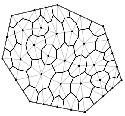
Figure 1: The dual mesh (black) is constructed by joining the centroids of the primal triangular mesh (grey). The volumes of these dual cells define the weights of an integration scheme based at the nodes of the primal mesh.

In order to complete the model specification, we must define an integration scheme to be used in (3). The simplest option is to attach to each node in the mesh a region $V_{i}$ for which the value of the basis function $\phi_{i}(s)$ is greater than the value of any other basis function. This construction, shown in Fig. 1, corresponds to the important notion of the dual mesh. The corresponding integration rule sets $\tilde{s}_{i}$ to be the node location and $\tilde{\alpha}_{i}=|V_{i}|$ to be the volume of the dual cell. This approximation, known as the midpoint rule, is second-order accurate on a regular grid but will be first-order accurate on an irregular mesh. We can use the structure of the mesh in other ways when constructing the integrator, for example constructing an integration scheme as the sum of optimal Gaussian integration rules on the individual triangles in the mesh. The weights and integration points for general triangles can be found in books on numerical analysis or finite element methods (Ern & Guermond, 2004). We discuss this further in the Appendix.

6 Convergence of the approximations

The proposed method (3) for approximating the likelihood in a log-Gaussian Cox process has two distinct approximations: one to the integral in the likelihood and another to the latent Gaussian random field. Here, we show that both of these converge. The proofs and more general statements of all of the results can be found in the Appendix.

The first aspect of the approximation, discussed in Section 4, replaces the intractable integral of the random intensity with a numerical quadrature scheme. The following theorem shows that, for any Gaussian random field $Z(\cdot)$, this approximation converges and the Hellinger distance between the true posterior distribution and the posterior distribution constructed from the approximate likelihood is bounded by the error in the integration scheme.

Theorem 6.1.

Assume that $Z(\cdot)$ has, almost surely, $k$ square-integrable derivatives, and that the $p$-point integration scheme in (3) has deterministic error of order $p^{-k}$. Then the Hellinger distance between the posterior distributions generated with the true and approximate likelihoods is $\mathcal{O}(p^{-k})$.

An interesting aspect of using stochastic partial differential equation models as our finite-dimensional Gaussian random field is that the prior distribution converges as the mesh is refined (Lindgren et al., 2011; Simpson et al., 2012b). This is distinct from predictive processes or fixed-rank kriging approaches, where the finite-dimensional model (2) is taken as the true underlying model. The convergence of this approximation was established by Lindgren et al. (2011). The following theorem refines this result and shows that the approximate posterior distribution converges weakly.

Theorem 6.2.

Assume that the observation window is a convex polygon in $\mathbb{R}^{2}$ and let $h$ be the maximum edge length in the mesh. Let $Z(\cdot)$ be the solution of (5) with $\alpha=2$. If $G(\cdot)$ is a uniformly Lipschitz continuous function, then the error in the posterior expectation ${E}\{G(Z)\mid y\}$ due to the stochastic partial differential equation approximation is of order $h^{1-\epsilon}$ for any $\epsilon>0$.

7 Examples

7.1 Log-Gaussian Cox processes with extensions

We consider the application of log-Gaussian Cox processes in three increasingly complicated situations. In the first, a log-Gaussian Cox process with covariates is fitted to a real data set observed everywhere in a rectangular area (Rue et al., 2009; Illian et al., 2012). The second example is a simulation study in the vein of Chakraborty et al. (2011), where the point pattern is incompletely observed due to varying sampling effort across the region of interest. The third case-study is inspired by the problem of mapping the risk associated with freak waves on oceans. We have constructed a point process defined only on the world’s oceans, i.e.,  over a very irregular, multiply-connected bounded region on a sphere. To the best of our knowledge, no other method can be practically extended to fit a log-Gaussian Cox process in this situation.

The examples are run using the R-INLA package (Rue et al., 2009; Martins et al., 2013) which implements both the stochastic partial differential equation models and the integrated nested Laplace approximation in the statistical computing language R (R Core Team, 2013). Wherever not specified otherwise, we use independent Gaussian prior distributions with mean $0$ and variance $100$ on $\log\kappa$ and $\log\tau$. In all examples, $\alpha=2$.

7.2 Comparison with a lattice-based approach for rainforest data

This case-study is a standard application of spatial point processes, associating species with soil properties in tropical rainforests. The complete data set consists of the location of all trees with diameter at breast height of 1cm or greater, for a total of $319$ tree species within a 50 ha rainforest plot on Barro Colorado Island in Panama that has never been logged. We model the large spatial pattern formed by 4294 trees of species Protium tenuifolium, shown in Fig. 2, relative to the covariate phosphorus, which is given on an interpolated grid (John et al., 2007; Hubbell et al., 1999; Condit, 1998). The plot on Barro Colorado Island is only one plot within a large network of 50 ha plots t established as part of an international effort to understand species survival and coexistence in species-rich ecosystems (Burslem et al., 2001).

Figure 2: The effect of soil potassium levels on the location of Protium tenuifolium. (a) The location of Protium tenuifolium; (b) The posterior covariate effect of phosphorus, using the standard lattice method (dashed), and the stochastic partial differential equation approach (solid).

Data sets with a similar structure have been analysed both with descriptive (Law et al., 2009) and model-based approaches (Waagepetersen, 2007; Waagepetersen & Guan, 2009; Wiegand et al., 2007). Integrated nested Laplace approximation can be used to fit a log-Gaussian Cox process to similar data, and also to a joint model of the pattern and covariates (Rue et al., 2009; Illian et al., 2012). For illustration, we fit a simple model, where the latent field is $Z(s)=\mu+\beta P(s)+x(s)$, where $\mu$ is a constant mean, $P(s)$ is a spatially varying covariate describing the level of phosphorus in the soil and $x(s)$ is an approximately intrinsic stochastic partial differential equation model with $\kappa=0.0014$, which corresponds to a range much larger than the spatial domain. The parameter $\log(\tau)$ is assigned a vague Gaussian prior distribution with mean zero and variance $1000$.

For comparison, we fit a lattice model with linear predictor $z=\mu 1+\beta P+x,$ where $1$ is a vector of ones, $P$ the phosphorus concentration, $x\sim N(0,\tau^{-1}Q^{-1})$ is an intrinsic second-order conditional autoregression (Rue & Held, 2005) and $\tau\sim Ga(1,10^{-5})$. Both models required around $25$ seconds to fit in R-INLA. The posterior means for the spatial random effects are shown in Fig. 3 and are centred at the same location. We believe the difference between the posterior distributions can be accounted for by the different prior distributions for $x$ and the different precision parameters. The posterior distribution for the effect of soil phosphorus on the locations of trees are shown in Fig. 2.

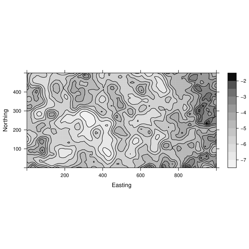
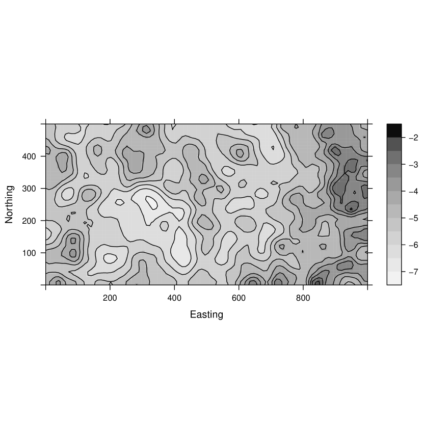
Figure 3: Estimated spatial effects for Protium tenuifolium: (a) Using a standard lattice point process model; (b) Using the stochastic partial differential equation approach.

7.3 Incorporating variable sampling effort

A major challenge when applying spatial point process models to real data sets is that the point pattern is rarely captured exactly, so sampling effort must be included in the observation process (Chakraborty & Gelfand, 2010; Chakraborty et al., 2011; Niemi & Fernandez, 2009). In this example, we consider the case where there is a sub-area in the data set with no measurements, but where presences are possible. This type of situation occurs, for instance, when considering the spatial distribution of an animal species over an area that contains a region that is impossible to survey (Elith et al., 2006). In a related situation, data sampling effort varies spatially and is higher in areas where the scientists expect a good chance of presence, as in preferential sampling models (Diggle et al., 2010).

Following Chakraborty et al. (2011), we include known sampling effort in our model by writing the intensity as $\lambda(s)=S(s)\exp\{Z(s)\}$, where $S(s)$ is a known function describing the sampling effort at location $s$. In this example, we assume that the point pattern has been observed perfectly, except in a rectangle where the pattern is not observed; see Fig. 4. We therefore define $S(s)$ to be zero inside this rectangle and unity everywhere else. It is straightforward to see from (1) that, with this choice of $S(s)$, the unsampled area does not contribute to the integral in the likelihood. We can therefore choose the mesh to be quite coarse in this area, as long as this does not adversely affect the stochastic partial differential equation approximation to the random field. Figure 4 shows a mesh that has been coarsened in a rectangular region corresponding to a hole in the sampling effort. When coarsening the mesh, it is important to remember that we still want small triangles in the vicinity of the observed region, and we want these to gradually change to larger triangles. This ensures that the stochastic partial differential equation approximation is stable. In Fig. 4 this transition can be clearly seen. The changes to the R-INLA code necessary to add sampling effort to basic point process code are minimal. This method can be extended in a straightforward manner to cover more complicated designs, although Chakraborty et al. (2011) suggest it is necessary to assume that the design is known.

In order to test our method on this type of problem, we simulated a log-Gaussian Cox process on $[-1,1]\times[-1,1]$ and removed the points from the rectangle $[-0.5,0.4]\times[-0.1,0.4]$ to simulate the variable sampling. The simulated data set is shown in Fig. 4, and the difference in the posterior mean generated from the full data and the censored data is shown in Fig. 5. There is very little difference between the two posterior means outside the censored area, whereas there are missing features within the censored area. We also compared the results obtained for two different meshes with the same maximum edge length, a regular lattice that covers the entire domain and contains $4225$ points, and the irregular mesh consisting of $3850$ points that is coarsened in the censored area, shown in Fig. 4. The posterior marginal distributions for the parameters for these two meshes are extremely similar. In order to avoid boundary effects in the finite-dimensional random field, it is important to have points inside the censored area to ensure that the random field behaves properly. Use of the mesh correctly adapted to the problem resulted in a significant decrease in computational time. With the regular grid, the full inference took $37$ seconds on a Linux laptop with a 2.2 GHz i7 4702HQ processor, whereas the computation on the irregular mesh required only $24$ seconds, a $35\%$ reduction by coarsening $11\%$ of the total mesh.

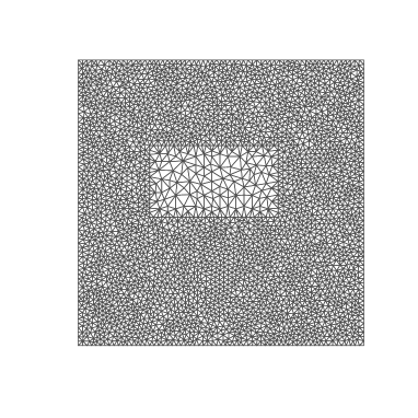
Figure 4: Simulated data with a hole in the sampling effort. (a) The inner rectangle borders the area in which there was no sampling, and the plusses show the points that were missed due to incomplete sampling; (b) A mesh that takes into account the lack of sampling effort in the rectangular region.

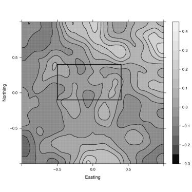
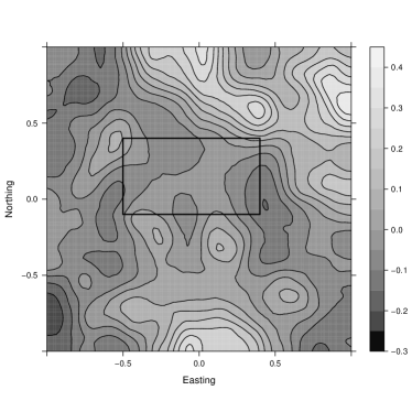
Figure 5: The posterior mean of the spatial effect for variable sampling effort (Section 7.3): (a) Using the complete simulated point pattern; (b) Using the incomplete, partially observed point pattern. The large scale features of both fields are similar in areas in which the point pattern was sampled.

7.4 A point process over the ocean

In applications, point processes often occur over complicated domains rather than rectangles, and the topology, topography and geometry of the domain will typically be meaningful when modelling the covariance structure, see the discussion of Wood et al. (2008) in the context of spatial smoothers. For this case-study, we have simulated a log-Gaussian Cox process on the oceans, motivated by a model for assessing the risk of freak waves.

The oceans form a non-convex, multiply-connected bounded region on the sphere and it is, therefore, necessary to construct a Gaussian random field model over this region. The main complication beyond those considered by Lindgren et al. (2011) is that we need a model for the covariance at the boundary. This difficult issue has been discussed very little in the statistics literature. As we are working with simulated data, we can choose a relatively simple, yet realistic, boundary model. We expect that wave heights vary more near the coast than in the deep ocean and, as the designation of a freak wave is relative to the expected wave height, the random field is defined using the Neumann boundary conditions, which approximately doubles the variance near the boundaries of the domain (Lindgren et al., 2011, Theorem 1).

The point process shown in Fig. 6 was constructed by simulating a Gaussian random field associated with the mesh in Fig. 6. The resulting point pattern has 913 points. Inference was performed on this model and the posterior mean is shown in Fig. 7. The posterior mean shows the same large-scale features as the sample used to generate the log-Gaussian Cox process, see Fig. 7, with the expected loss of information due to the uninformative nature of point pattern data.

Effects induced by the boundary conditions can be seen in Fig. 8. The pointwise posterior standard deviation of the latent Gaussian field is shown in Fig. 8. The standard deviation is reasonably constant away from the coasts, but is much higher near the boundaries. There are some interesting effects in the Gulf of Carpentaria in Australia, and in the North Sea. This is an effect of the prior model, which increases the variance near the boundaries and in areas with high curvature of the coastline.

In the context of freak wave modelling, the most important result is displayed in Fig. 8, showing the probability that the log-risk will be greater than $5.5$. Once again we see pronounced effects near the coastlines. This type of map can easily be computed using the function inla.pmarginal in the R-INLA package. It is also possible to use the excursions package (Bolin & Lindgren, 2015) in R to construct joint exceedance maps.

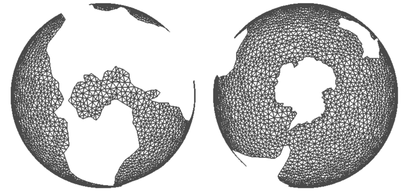
Figure 6: (a) A simulated log-Gaussian Cox processes over the oceans; (b) A mesh that covers the oceans.

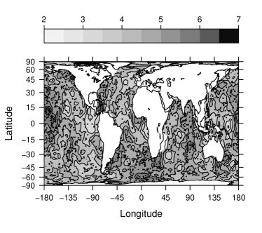
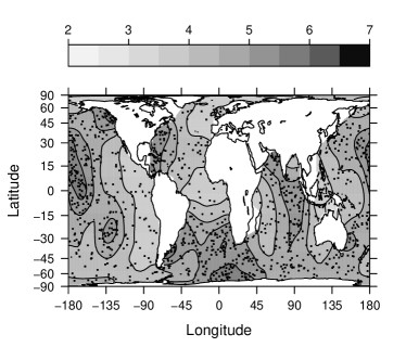
Figure 7: Inference for a point process over the oceans. (a) True surface from the latent Gaussian random field used to generate the sample in Fig. 6; (b) Posterior mean of the latent spatial effect. Note that the large scale behaviour is the same for both figures.

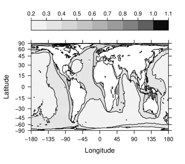
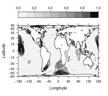
Figure 8: Inference for a point process over the oceans. (a) The pointwise posterior standard deviation for the log risk surface; (b) The posterior risk map $\rm{pr}\log\lambda(s)>5.5\mid y\}$.

8 Discussion and future work

The approximation to analyse log-Gaussian Cox processes introduced in this paper is valid also when using kernel methods (Higdon, 1998), predictive processes (Banerjee et al., 2008) or fixed-rank kriging (Cressie & Johannesson, 2008). The problem with using these methods in the given context is that their basis functions are typically non-local and, therefore, the point evaluation matrices $A_{i}$ in (4) are dense; see Simpson et al. (2012b) for a further discussion of the choice of basis functions in spatial statistics.

In Section 7.4, we consider a point process over a complicated region of the sphere. To the best of our knowledge, there are no other applicable inference methods for this example that include a covariance model at the boundaries. In general, modelling of boundary effects for point processes has not previously been discussed in the literature. We argue that by using Neumann, or no-flux, boundary conditions the variance at the boundaries increases. Similarly, Dirichlet boundary conditions, which correspond to fixing the value of the field at the boundaries, decrease the variance. A future question is to construct good boundary models, and study their effect in a statistical context.

There is work to be done on the theoretical properties of the approximation presented in this paper. Some partial results are given in the Appendix, but they are not the complete story. In particular, it would be interesting to study the effect of both the likelihood approximation and the finite-dimensional approximation of the hyper-parameters of the model. These parameters, which control range, variance and, in more complicated cases, non-stationarity, are often of scientific interest and determining the rate of convergence will help us understand their interpretations.

Moving our considerations to more general finite-dimensional expansion (2), it is also of interest to quantify the link between the basis functions $\phi_{i}(s)$ and the statistical properties of the estimator. Although there has been work by Stein (2014), there are a number of open questions. This is a challenging problem as the interest is in non-asymptotic behaviour both in the number of basis functions and in the amount of data. In order to do practical spatial statistics, we need to give something up and often methods will be asymptotically incorrect. However, it may be that in realistic regimes, the resulting statistical error is manageable.

Finally, the approximation in Section 4 applies even when the latent random field $Z(s)$ is not Gaussian. The only requirement is that it has the basis function expansion (2) and that the statistical properties of $z$ are known. In particular, this approximation applies to stochastic partial differential equation models with non-Gaussian noise. This has been investigated for type-$G$ Lévy processes, and especially for Laplace random fields (Bolin, 2014). Similarly, replacing Gaussian white noise with Poisson noise would result in shot-noise Cox process models of the Matérn type. It may be possible to avoid the assumptions that the random field is Gaussian in the Appendix. The main use of Gaussianity is in the form of Fernique’s theorem, which is a statement about the tails of a Gaussian random field and it is possible that similar results would hold for non-Gaussian fields after modifying the growth conditions on the likelihood and the functionals.

Appendix

.1 Likelihood approximation

Throughout this appendix, we assume that the parameters in the covariance model for $Z(s)$ are known and fixed. We show that, for a fixed random field $Z(s)$, the posterior distribution computed using the likelihood approximation converges strongly to the true posterior distribution, and the rate of convergence can increase as the smoothness of the field increases. We also show that for either the true or approximate likelihood, the posterior distribution generated using the finite-dimensional stochastic partial differential equation model converges weakly to that generated using the limiting Matérn model. Finally, we show that under further assumptions the convergence rate depends both on the basis functions and the smoothness of the underlying random field. The main tools used in this appendix come from the inverse problems literature, surveyed in Stuart (2010), which deals with inference of indirectly observed continuous Gaussian random fields.

In order to show that the approximate posterior distributions converge to the true posterior distribution, it is useful to re-write the problem in terms of measures. Let $\mu_{0}(A)=\mbox{pr}\{Z(\cdot)\in A\}$ be the Gaussian measure defined by the Gaussian random field prior measure on $Z(\cdot)$. If we define

$$\Phi(Z;Y)=\int_{\Omega}\exp\{Z(s)\}\,ds-\sum_{s_{i}\in Y}Z(s_{i}),$$

then the posterior probability measure $\mu$ for $Z(\cdot)$ conditioned on $Y$ can be defined through its Radon–Nikodym derivative $\nicefrac{{d\mu}}{{d\mu_{0}}}(Z)\propto M^{-1}\exp\{-\Phi(Z;Y)\},$ where $M$ is a normalising constant required to ensure that $\mu$ is a probability measure. We can, in a similar fashion, define the approximate posterior measure as

$$\frac{d\mu^{p}}{d\mu_{0}}(Z)\propto M_{p}^{-1}\exp\{-\Phi^{p}(Z;Y)\},$$ (7)

where $\Phi^{p}(Z;Y)=\sum_{i=1}^{p}\tilde{\alpha}_{i}\exp\{Z(\tilde{s}_{i})\}-\sum_{s_{i}\in Y}Z(s_{i}),$ and $M_{p}$ is a normalising constant. Cotter et al. (2010) showed that, under conditions $\Phi$ and $\Phi^{p}$, the Hellinger distance

$$d_{\text{Hell}}\left(\mu,\mu^{p}\right)=\left[\frac{1}{2}\int\left\{\left({\frac{d\mu}{d\mu_{0}}}\right)^{1/2}-\left({\frac{d\mu^{p}}{d\mu_{0}}}\right)^{1/2}\right\}^{2}\,d\mu_{0}\right]^{1/2}$$

between the approximate and true posterior distributions converges to zero. Stuart (2010) notes that convergence in Hellinger distance implies convergence in the total variation metric and it can be related to convergence of functionals using the identity

$$\left\lvert E_{\mu}\{f(Z)\}-E_{\mu^{\prime}}\{f(Z^{\prime})\}\right\rvert\leq 2\left[E_{\mu}\{|f(Z)|^{2}\}-E_{\mu^{\prime}}\{|f(Z^{\prime})|^{2}\}\right]d_{\text{Hell}}(\mu,\mu^{\prime}).$$ (8)

The following theorem shows that their theory applies to our approximate likelihood.

Theorem .1.

Consider a Gaussian random field $Z(\cdot)$ defined on a Lipschitz domain $\Omega$ and assume that its paths are almost surely in the Sobolev space $H^{\alpha}(\Omega)$ with $\alpha>d/2$. Assume that the integration rule satisfies

$$\left|\int_{\Omega}f(s)\,ds-\sum_{i=1}^{p}\tilde{\alpha}_{i}f(\tilde{s}_{i})\right|\leq C\psi(p)\lVert f\rVert_{H^{\gamma}},$$ (9)

where $\psi(p)\rightarrow 0$ as $p\rightarrow\infty$ and $\gamma\leq\alpha$. Then, as $p\rightarrow\infty$, $d_{\text{Hell}}\left(\mu,\mu^{p}\right)\rightarrow 0$. Furthermore, if $\gamma$ is an integer, then $d_{\text{Hell}}\left(\mu,\mu^{p}\right)\leq C\psi(p).$

Proof .2.

This result follows directly from Theorem 2.4 of Cotter et al. (2010) if we can show that the potential is bounded above and below and that the error in the likelihood approximation is integrable. Let $\lVert Z(\cdot)\rVert_{\infty}=\sup_{s\in\Omega}|Z(s)|$, and let $\lVert Y\rVert$ be the number of points in the point pattern $Y$. Firstly we note that, by assumption, $\lVert Z(\cdot)\rVert_{\infty}$ and $\lVert Y\rVert$ are almost surely finite. Then, if $\max(\lVert Z\rVert_{\infty},\lVert Y\rVert)<r$, straightforward calculation shows that $\Phi(Z;Y)\leq|\Omega|e^{r}+r^{2}.$ Similarly, when $\lVert Y\rVert<r$,

$$\Phi(Z;Y)=\int_{\Omega}\exp\{Z(s)\}\,ds-\sum_{s_{i}\in Y}Z(s_{i})\geq-r\lVert Z\rVert_{\infty}\geq-Cr\lVert Z\rVert_{H^{\gamma}},$$

where the last inequality follows from Sobolev’s embedding theorem and is true for every $\gamma>d/2$. Similar arguments show that $\Phi^{p}(Z;Y)$ is also bounded above and below independently of $p$.

To show that the error in the likelihood induces a similar error in the posterior distribution, we need to verify that, for sufficiently small $\epsilon>0$, there exists a $K>0$ that does not depend on $Z$ such that $\left|\Phi(Z;Y)-\Phi^{p}(Z;Y)\right|\leq K\exp\left(\epsilon\lVert Z\rVert_{\infty}^{2}\right)\psi(p).$ By assumption, this reduces to showing that $\lVert\exp\{Z(\cdot)\}\rVert_{H^{\gamma}}\leq K\exp(\epsilon\lVert Z\rVert_{\infty}^{2})$ for large enough $Z$. Let $\gamma$ be an integer. Now, for any realisation of $Z(\cdot):D\rightarrow\mathbb{R}$, there exists an extension $IZ(\cdot):\mathbb{R}^{d}\rightarrow\mathbb{R}$ such that $IZ(\cdot)\in H^{\gamma}(\mathbb{R}^{d})$ has compact support and $\left.IZ\right\rvert_{D}(\cdot)=Z(\cdot)$. Using the quotient space structure of a Sobolev space on a domain, it follows that

$$\lVert\exp\{Z(\cdot)\}\rVert_{H^{\gamma}(\Omega)} =\inf_{H^{\gamma}(\mathbb{R}^{d})\ni\tilde{Z}(s)=Z(s),\;a.s.\;s\in D}\lVert\exp\{\tilde{Z}(\cdot)\}\rVert_{H^{\gamma}(\mathbb{R}^{d})}$$

$$\leq C\exp(\lVert IZ(\cdot)\rVert_{L^{\infty}(\mathbb{R}^{d})})\left(\lVert IZ(\cdot)\rVert_{H^{\gamma}(\mathbb{R}^{d})}+\lVert IZ(\cdot)\rVert_{H^{\gamma}(\mathbb{R}^{d})}^{\gamma}\right)$$

$$\leq C\exp(C\lVert Z(\cdot)\rVert_{\infty})\left(\lVert Z(\cdot)\rVert_{H^{\gamma}(\Omega)}+\lVert Z(\cdot)\rVert_{H^{\gamma}(\Omega)}^{\gamma}\right),$$

where the first inequality follows from Theorems 2 and 3 of Bourdaud & Sickel (2010), the second inequality follows from the boundedness of the extension operator and the constant $C$ changes from line to line.

Remark .3.

The condition that $\gamma$ is an integer can probably be relaxed, but it is an open question whether $\lVert\exp\{Z(s)\}\rVert_{H^{\gamma}(\mathbb{R}^{d})}$ can be bounded for non-integer $\gamma$ in the same way as in the integer case. If this was true, it would suggest the use of integration rules of order $\lceil{\alpha}\rceil$ rather than $\lfloor{\alpha}\rfloor$ and would slightly improve the convergence rate.

The techniques used to prove Theorem .1 also allow us to give a more informative convergence result for the traditional counting process approximation to the log-Gaussian Cox process than those considered by Waagepetersen (2004).

Corollary .4.

Assume $\alpha\geq 2$. Then the classical $(p+1)\times(p+1)$ lattice approximation to the log-Gaussian Cox process converges in the Hellinger distance at a rate of $\mathcal{O}(p^{-1})$.

Proof .5.

For simplicity, we will assume that the observation window $D$ is square and the lattice is equally spaced in both directions. The lattice approximation is of the form (7) with

$$\Phi^{p}(Z)=\sum_{i,j=1}^{p}|S_{ij}|\exp\{Z(\tilde{s}_{ij})\}-\sum_{i,j=1}^{p}\lVert Y\cap S_{ij}\rVert Z(\tilde{s}_{ij}),$$ (10)

where $S_{ij}$ is the $(i,j)$ lattice cell and $\tilde{s}_{ij}$ is the centroid of $S_{ij}$. The first term in (10) is the midpoint rule approximation to $\int_{\Omega}\exp\{Z(s)\}\,ds$, which, due to the regularity of the lattice satisfies (9) with $\psi(p)=p^{-\gamma}$ $(d/2<\gamma\leq 2)$, (Theorem 8.5, Ern & Guermond, 2004). The error in the likelihood arising from the approximation of $Z(s_{k})$ by $Z(\tilde{s}_{ij})$ for any $s_{k}\in Y\cap S_{ij}$ can be bounded using Taylor’s theorem as $\left|Z(s_{k})-Z(\tilde{s}_{ij})\right|\leq p^{-1}\sup_{s\in S_{ij}}\sup_{\ell=1,\ldots,d}\left|\frac{\partial Z(s)}{\partial s_{\ell}}\right|\leq Cp^{-1}\lVert Z\rVert_{H^{1+d/2}(S_{ij})},$ where the second inequality is a consequence of Sobolev’s embedding theorem (Brenner & Scott, 2007, Corollary 1.4.7). It follows using the arguments in the proof of Theorem .1 that for a two-dimensional lattice, $\left|\Phi(Z)-\Phi^{p}(Z)\right|\leq C\lVert Y\rVert p^{-1}\lVert Z\rVert_{H^{2}(\Omega)}$, and the result follows from Theorem 2.4 of Cotter et al. (2010).

Remark .6.

Examining the proof of Corollary A.4, it can be seen that the rate of convergence is determined by the binning procedure and using the lattice quadrature rule and the approximate likelihood proposed in this paper the rate of convergence would be $\mathcal{O}(p^{-2})$ for smooth enough fields.

.2 Random field approximation

While Appendix .1 shows that for fixed $Z(\cdot)$ the likelihood approximation introduced in this paper converges, this is not enough to show that the posterior distributions computed in Section 7 converge as we are simultaneously approximating the log-Gaussian Cox process likelihood and the Gaussian random field using the approximation outlined in Section 5. In this appendix, we close this gap when the hyperparameters are fixed and show the convergence of a general class of finite-dimensional approximations to problems in which the indirectly observed unknown random function is equipped a priori with a Gaussian random field.

There are a number of technical challenges to showing convergence of this approximation. The first is that we need to compare a measure on an infinite-dimensional space with a sequence of measures on different finite-dimensional spaces. We will, therefore, no longer be able to consider convergence in the Hellinger metric, but rather we will consider a weaker mode of convergence of an approximating measure $\nu^{n,p}$ to $\mu$, that is the convergence of functionals of the form $\int G(Z_{n})\,d\nu^{n,p}(Z_{n})\rightarrow\int G(Z)\,d\mu(Z),$ for Lipschitz continuous functions that satisfy a growth condition to ensure the functionals are finite. This is slightly stronger than convergence in distribution, for which bounded Lipschitz functions suffice (Bogachev, 2007, Section 8.3). When the finite-dimensional approximation to the Gaussian random field is computed by truncating its Karhunen–Loève expansion, Dashti & Stuart (2011) showed convergence. Their techniques, which relied heavily on the idea that truncation of the Karhunen–Loève expansion is an $L^{2}(\Omega)$ projection, are not directly applicable to the approximation outlined in Section 5.

In Section .3, we extend Theorem 2.6 of Dashti & Stuart (2011) to a general class of finite-dimensional approximations. In particular we show that if the approximation $Z_{n}(\cdot)$ to $Z(\cdot)$ is stable, in the sense that $\lVert Z_{n}\rVert_{H}\leq C\lVert Z\rVert_{H}$ uniformly in $n$, then the convergence of the functionals is governed by the deterministic error in the pathwise approximation. In Section .4 we show that for approximations of the general form of the stochastic partial differential equation approximation, this error is controlled by the ability of the finite-dimensional basis functions to approximate realisations of the true prior model. These results mirror previous quantitative results (Simpson et al., 2012a, b; Bolin & Lindgren, 2013), in which the stable, convergent approximation properties of piecewise linear functions were used to argue for the adoption of stochastic partial differential equation models.

.3 A general result on the convergence of finite-dimensional approximations

Let $V\subset H$ be Banach spaces and assume that $\lVert\cdot\rVert_{H}\leq C\lVert\cdot\rVert_{V}$. Assume that the Gaussian random field $Z(\cdot)$ has paths almost surely in $V$ and define the approximate random field $Z_{n}(\cdot)=R_{n}Z(\cdot)$, where $R_{n}:V\rightarrow V_{n}$ is a deterministic linear operator, and $V_{n}\subset H$ is an $n$–dimensional vector space that is not necessarily a subspace of $V$. In the special case that $V_{n}\subset V$ and $R_{n}$ is a projector, the arguments of Dashti & Stuart (2011) can be used to show convergence.

Extending the notation from Appendix .1, we define $\mu_{0}(\cdot)$ to be the law of $Z(\cdot)$ and consider the infinite-dimensional posterior distribution $\nu(\cdot)$ defined by $\nicefrac{{d\mu}}{{d\mu_{0}}}=M^{-1}\exp\{-\Phi(Z;Y)\}.$ Similarly, we define the law of $Z_{n}(\cdot)$ to be $\nu_{0}^{n}(\cdot)$ and define the approximate posterior distributions $\nu^{n,p}$ as $\nicefrac{{d\nu^{n,p}}}{{d\nu_{0}^{n}}}=M_{n,p}^{-1}\exp\{-\Phi^{p}(Z_{n};Y)\},$ where $M_{n,p}$ is a normalising constant. We make the following assumptions on the potential $\Phi(\cdot;Y)$ (Dashti & Stuart, 2011).

Consider the potential function $\Phi(\cdot;Y):H\rightarrow\mathbb{R}^{+}$. Assume that for every $\epsilon>0$ and $r>0$, $\lVert Y\rVert<r$ and there exists a $C=C(\epsilon,r)>0$, which may change from line to line, such that, for all $Z\in H$, $\exp\{-\Phi(Z;Y)\}\leq C\exp(\epsilon\lVert Z\rVert_{H}^{2}).$ Also, for every $Z\in H$, where $\lVert Z\rVert_{H}<r$, $\Phi(Z;Y)\leq C$ and for every $Z_{1},Z_{2}\in H$, $|\Phi(Z_{1};Y)-\Phi(Z_{2};Y)|\leq C\exp\left\{\epsilon\max(\lVert Z_{1}\rVert_{H}^{2},\lVert Z_{2}\rVert_{H}^{2})\right\}\lVert Z_{1}-Z_{2}\rVert_{H}.$

The following theorem says that for nice functionals, the error in the approximation depends on how well the approximate random field $Z_{n}(\cdot)$ approximates the true random field in a pathwise sense as well as on the quality of the likelihood approximation. While the argument holds mutatis mutandis for Banach space-valued functionals $G$ (see Dashti & Stuart, 2011), for simplicity we restrict ourselves to real-valued functionals.

Theorem .7.

Assume that Assumption .3 holds for $\Phi(\cdot;Y)$, $\Phi^{p}(\cdot;Y)$ and $\Phi^{n,p}(\cdot;Y)=\Phi^{p}(R_{n}\cdot;Y)$ uniformly in $n$ and $p$. Let $G$ be a Lipschitz continuous function such that, for every $\epsilon>0$, there exists a $C=C(\epsilon)\in(0,\infty)$ such that, for every $Z_{1}\in V$ and $Z_{2}\in H$, $|{G(Z_{1})-G(Z_{2})}|\leq C\exp\left\{\epsilon\max(\lVert Z_{1}\rVert^{2}_{V},\lVert Z_{2}\rVert^{2}_{H})\right\}\lVert Z_{1}-Z_{2}\rVert_{H}.$ If the restriction operator $R_{n}$ satisfies the stability estimate

$$\lVert R_{n}Z(\cdot)\rVert_{H}\leq C\lVert Z(\cdot)\rVert_{V},$$ (11)

for all $Z(\cdot)\in V,$ then

$$e_{G}=|E_{\mu}\{G(Z)\}-E_{\nu^{n,p}}\{G(Z_{n})\}|\leq C\left\{\sup_{Z(\cdot)\in V}\frac{\lVert Z(\cdot)-R_{n}Z(\cdot)\rVert_{H}}{\lVert Z(\cdot)\rVert_{V}}+\psi(p)\right\}.$$

Proof .8.

Using the notation of Appendix .1, it follows that

$$e_{G} \leq\left|E_{\mu}\{G(Z)\}-E_{\mu^{p}}\{G(Z)\}\right|+\left|E_{\mu^{p}}\{G(Z)\}-E_{\nu^{n,p}}\{G(Z_{n})\}\right|\equiv B_{1}+B_{2}$$

and it follows from Theorem A.1 and (8) that $B_{1}\leq C\psi(p)$. Let $Z\sim\mu_{0}(\cdot)$ and construct the coupling $(Z,Z_{n})\in V\times V_{n}$ through the identity $Z_{n}=R_{n}Z$. It follows that

$$B_{2} =\left|M_{p}^{-1}\int_{V}G(Z)\exp\{-\Phi^{p}(Z)\}\,d\mu_{0}-M_{n,p}^{-1}\int_{V_{n}}G(Z_{n})\exp\{-\Phi^{p}(Z_{n})\}\,d\nu^{n}_{0}\right|$$

$$\leq M_{p}^{-1}\left|\int_{V}G(Z)\exp\{-\Phi^{p}(Z)\}\,d\mu_{0}-\int_{V_{n}}G(Z_{n})\exp\{-\Phi^{p}(Z_{n})\}\,d\nu^{n}_{0}\right|$$

$$\quad+\left|M_{p}^{-1}-M_{n,p}^{-1}\right|\int_{V_{n}}|G(Z_{n})|\exp\{-\Phi^{p}(Z_{n})\}\,d\nu^{n}_{0}\equiv B_{3}+B_{4}.$$

The normalising constants $M_{p}$ and $M_{n,p}$ are bounded both above and below uniformly in $n$ (Theorems 4.1 and 4.2, Stuart, 2010).

Let $\lambda(\cdot,\cdot)$ be the law of the coupling $(Z,Z_{n})$. Then, for any $\epsilon>0$,

$$M_{p}B_{3} =\left|\int_{V\times V_{n}}\left[G(Z)\exp\{-\Phi^{p}(Z)\}-G(Z_{n})\exp\{-\Phi^{p}(Z_{n})\}\right]\,d\lambda(Z,Z_{n})\right|$$

$$\leq\int_{V\times V_{n}}|G(Z)|\left|\exp\left\{-\Phi^{p}(Z)\}-\exp\{-\Phi^{p}(Z_{n})\right\}\right|+\exp\{-\Phi^{p}(Z_{n})\}\left|G(Z)-G(Z_{n})\right|\,d\lambda(Z,Z_{n})$$

$$\leq C\int_{V\times V_{n}}\exp\left\{2C\epsilon\lVert Z\rVert_{V}^{2}+\epsilon\max(\lVert Z\rVert_{V}^{2},C\lVert Z\rVert^{2}_{V})\right\}\lVert Z-Z_{n}\rVert_{H}\,d\lambda(Z,Z_{n})$$

$$\leq C\left(\sup_{Z(\cdot)\in V}\frac{\lVert Z(\cdot)-R_{n}Z(\cdot)\rVert_{H}}{\lVert Z(\cdot)\rVert_{V}}\right)\int_{V\times V_{n}}\exp(3C\epsilon\lVert Z\rVert_{V}^{2})\lVert Z\rVert_{V}\,d\lambda(Z,Z_{n})$$

$$\leq C\sup_{Z(\cdot)\in V}\frac{\lVert Z(\cdot)-R_{n}Z(\cdot)\rVert_{H}}{\lVert Z(\cdot)\rVert_{V}},$$

where the second inequality follows from standard bounds on the exponential function, the assumptions on $\Phi^{p}(\cdot)$ and $G(\cdot)$, and the stability assumption (11). The third inequality follows from the observation that $Z_{n}=R_{n}Z$ almost surely, $Z(\cdot)\in V$ almost surely and the embedding $\lVert\cdot\rVert_{H}\leq C\lVert\cdot\rVert_{V}$, and the final inequality follows from Fernique’s theorem, which ensures that the expectation is finite (Stuart, 2010).

To bound $B_{4}$, we first note that $\int_{V_{n}}|G(Z_{n})|\exp\{-\Phi^{p}(Z_{n})\}\,d\nu^{n}_{0}<\infty$ uniformly in $n$ by assumption and Fernique’s theorem. Then it is enough to note that

$$\left|M_{p}^{-1}-M_{n,p}^{-1}\right|\leq\max\left(M_{p}^{-2},M_{n,p}^{-2}\right)\left|M_{n}-M_{n,p}\right|$$

$$\qquad\leq C\int_{V\times V_{n}}\left|\exp\{-\Phi^{p}(Z)\}-\exp\{-\Phi^{p}(Z_{n})\}\right|\,d\lambda(Z,Z_{n})\leq C\sup_{Z(\cdot)\in V}\frac{\lVert Z(\cdot)-R_{n}Z(\cdot)\rVert_{H}}{\lVert Z(\cdot)\rVert_{V}},$$

using the reasoning above.

.4 Convergence of the stochastic partial differential equation approximation

In order to apply Theorem .7 to stochastic differential equation models, it is useful to consider the abstract version of the approximation outlined in Section 5. Let $L:H\rightarrow L^{2}(\Omega)$ be an operator and define the random field $Z(\cdot)$ through the equation $LZ(\cdot)=W(\cdot).$ Then $Z(\cdot)$ is a Gaussian random field over the sample space $H$ with covariance operator $C=L^{-1}L^{-*}$, where the star denotes the adjoint operator. If $L_{n}:H\rightarrow L^{2}(\Omega)$ is the Galerkin approximation to $L$ over $V_{n}$ defined by $\langle\phi,L_{n}\psi\rangle_{H}=\langle\phi,L\psi\rangle_{H}$ for all $\phi,\psi\in V_{n}$, then the corresponding approximate Gaussian random field $Z_{n}(\cdot)$ has covariance operator given by $C_{n}^{\dagger}=L_{n}^{*}L_{n}$, where $C^{\dagger}$ is the pseudoinverse of $C$ satisfies $C^{\dagger}H\perp_{H}V_{n}$. With this setup in mind, the restriction operator $R_{n}$ is defined by the equation $C_{n}=R_{n}CR_{n}^{*}$, from which it can be seen that $R_{n}=L_{n}^{\dagger}L$ is a natural choice. If $Z_{n}(\cdot)$ converges in distribution to $Z(\cdot)$, which is the case for the models in Section 5 (Lindgren et al., 2011), we can use Skorohod’s representation theorem to construct, possibly on a different probability space, the coupling $(Z,Z_{n})$, defined by $Z_{n}(\cdot)=R_{n}Z(\cdot)$ almost surely, that is required in Theorem A.7. Hence

$$\sup_{Z(\cdot)\in V}\frac{\lVert Z(\cdot)-R_{n}Z(\cdot)\rVert_{H}}{\lVert Z(\cdot)\rVert_{V}}=\sup_{f(\cdot)\in LV}\frac{\lVert L^{-1}f(\cdot)-L_{n}^{{\dagger}}g(\cdot)\rVert_{H}}{\lVert L^{-1}f(\cdot)\rVert_{V}}$$ (12)

and the rate of convergence is governed by how well solutions to the partial differential equation $Lx(\cdot)=f(\cdot)$ can be approximated by solutions to $L_{n}x_{n}(\cdot)=f(\cdot)$.

The following Theorem shows that, for fixed parameters, the approximate posterior distributions computed using the stochastic partial differential equation approach introduced by Lindgren et al. (2011) converge.

Theorem .9.

Let $\Omega\in\mathbb{R}^{2}$ be a convex polygon. Let $G$ be a Lipschitz continuous function that satisfies the assumptions of Theorem A.7. Assume that $\kappa>0$ and the family of triangulations $\mathcal{T}_{n}$ is quasi-uniform (Definition 4.4.13 Brenner & Scott, 2007). Then, if the approximate posterior measure $\nu^{n,p}$ is defined using the approximation and the integration rule outlined in Section 5, then, for any $\epsilon>0$, $e^{p}_{G}=\left|E_{\mu^{p}}\{G(Z)\}-E_{\nu^{n,p}}\{G(Z_{n})\}\right|\leq Ch^{1-\epsilon},$ where $h$ is the length of the largest edge in the mesh.

Proof .10.

The use of Theorem A.7 is complicated by the lack of Sobolev regularity of the Gaussian random field. In particular, the field $Z(s)$ considered in Section 5 is almost surely in $V=H^{1-\epsilon}(\Omega)$ for all $\epsilon>0$ (Lemma 6.2.7 Stuart, 2010). We then take $V=L^{2}(\Omega)$ and define the differential operator as $L=\kappa^{2}-\Delta$. We define the approximation space $V_{n}$ to be the space of piecewise linear functions defined over the triangulation $T_{n}$ and let $h$ be the maximum edge length. Under the assumptions on $\Omega$, $LV=H^{-1-\epsilon}(\Omega)$ (Ern & Guermond, 2004, 3.12), where a Sobolev space with negative index is defined as the dual of the space with the corresponding positive index. This is consistent with the fact that white noise can be considered a random function in $H^{-1-\epsilon}(\Omega)$ (Walsh, 1986). In order to define $L_{n}$, we need the $L^{2}(\Omega)$–orthogonal projector $P_{n}:H\rightarrow V_{n}\equiv\mathbb{R}^{n}$ and we define the Galerkin approximation as $L_{n}^{-1}=P_{n}^{*}(\kappa^{2}C_{n}+G_{n}-B_{n})^{-1}P_{n}$.

Fix $\epsilon\in(0,\frac{1}{2})$ and $f\in H^{-1-\epsilon}$ and let $z$ be the distributional solution to $Lz=f$. We emphasise that $f(\cdot)$ is not a function in an ordinary sense, but a distribution, and in the remainder of this proof integrals containing $f\in H^{-s}(\Omega)$ ($s>0$) should be interpreted as $\int_{\Omega}f(s)\phi(s)\,ds\equiv\langle f,\phi\rangle_{H^{-s}(\Omega),H^{s}(\Omega)},$ where the angle brackets denote the duality pairing.

As the standard convergence theory for finite element methods (Brenner & Scott, 2007; Ern & Guermond, 2004), would require the sample paths to be almost surely in $H^{2}(\Omega)$, we modify the arguments used to prove Proposition 1 in Scott (1976). The crucial step in Scott’s method is to approximate $f(s)$ by a piecewise linear function $f_{n}(s)$ defined over $T_{n}$ such that $\lVert f_{n}\rVert_{L^{2}(\Omega)}$ is controlled by a negative power of $h$. We define $f_{n}(s)$ as $\int_{\Omega}f_{n}(s)v_{n}(s)\,ds=\int_{\Omega}f(s)v_{n}(s)\,ds$ for all $v_{n}\in V_{n}$, where the second integral is understood in the sense of distributions and makes sense because $V_{n}\subset H^{1+\epsilon}(\Omega)$ (Belgacem & Brenner, 2001). For an arbitrary $v\in L^{2}$, let $v_{n}\in V_{n}$ be the orthogonal projection of $v$ onto $V_{n}$. Then

$$\int_{\Omega}f_{n}(s)v(s)\,ds=\int_{\Omega}f(s)v_{n}(s)\,ds\leq\lVert f\rVert_{H^{-1-\epsilon}(\Omega)}\lVert v_{n}\rVert_{H^{1+\epsilon}(\Omega)}\leq Ch^{-1-\epsilon}\lVert f\rVert_{H^{-1-\epsilon}(\Omega)}\lVert v\rVert_{L^{2}(\Omega)},$$

where the final inequality follows from equations (1.5) and (1.6) of Belgacem & Brenner (2001). As $v$ was arbitrary, this gives an appropriate bound for $\lVert f_{n}\rVert_{L^{2}(\Omega)}$.

Define $\tilde{z}(s)\in H^{2}(\Omega)$ to be the solution of $\int_{\Omega}\nabla\tilde{z}(s)\nabla\phi(s)\,ds=\int_{\Omega}f_{n}(s)\phi(s)\,ds$ for all $\phi\in H^{1}(\Omega)$ and consider the finite element approximation $z_{n}\in V_{n}$ defined as $\int_{\Omega}\nabla{z}_{n}(s)\nabla\phi_{n}(s)\,ds=\int_{\Omega}f_{n}(s)\phi_{n}(s)\,ds$ for all $\phi_{n}\in V_{n}.$ The dependence of $\tilde{z}$ on $n$ is suppressed for readability. The key observation is that $z_{n}(s)$ can be considered a finite element approximation to both $z(s)$ and $\tilde{z}(s)$ as $\int_{\Omega}f_{n}(s)\phi_{n}(s)\,ds=\int_{\Omega}f(s)\phi_{n}(s)\,ds$ for every $\phi_{n}\in V_{n}$. It follows from standard finite element theory (Brenner & Scott, 2007, Theorem 5.7.6) that

$$\lVert\tilde{z}-z_{n}\rVert_{L^{2}(\Omega)}\leq Ch^{2}\lVert\tilde{z}\rVert_{H^{2}(\Omega)}\leq Ch^{2}\lVert f_{n}\rVert_{L^{2}}(\Omega)\leq Ch^{1-\epsilon}.$$

The final ingredient of the proof is to bound $\lVert z-\tilde{z}\rVert_{L^{2}(\Omega)}$. Fix $\phi(s)\in L^{2}(\Omega)$ and let $\Phi(s)$ be the solution to $L^{*}\Phi=\phi$, where $L^{*}$ is the adjoint of $L$. Then it follows that, for any $v_{n}\in V_{n}$,

$$\int_{\Omega}\{z(s)-\tilde{z}(s)\}\phi(s)\,ds =\int_{\Omega}\{z(s)-\tilde{z}(s)\}L^{*}\Phi(s)\,ds=\int_{\Omega}L\{z(s)-\tilde{z}(s)\}\Phi(s)\,ds$$

$$=\int_{\Omega}\{f(s)-f_{n}(s)\}(\Phi(s)-v_{n})\,ds$$

$$\leq C\lVert f\rVert_{H^{-1-\epsilon}(\Omega)}h^{-1-\epsilon}\inf_{v_{n}\in V_{n}}\left(h^{1+\epsilon}\lVert\Phi-v_{n}\rVert_{H^{1+\epsilon}(\Omega)}+\lVert\Phi-v_{n}\rVert_{L^{2}(\Omega)}\right)$$

$$\leq C\lVert f\rVert_{H^{-1-\epsilon}(\Omega)}h^{-1-\epsilon}h\lVert\Phi\rVert_{H^{2}(\Omega)}\leq C\lVert f\rVert_{H^{-1-\epsilon}(\Omega)}h^{1-\epsilon}\lVert\phi\rVert_{L^{2}(\Omega)},$$

where the second line follows from the orthogonality of $f-f_{n}$ to $V_{n}$, the penultimate inequality follows from Theorem 14.4.2 of Brenner & Scott (2007) and the fact that $\Phi\in H^{2}(\Omega)$. As $\phi(s)$ was arbitrary, this completes the proof.

Unfortunately we are unable to prove that the entire posterior distribution converges. This is due to the gap in the theory identified in Remark A.3, which prevents Theorem A.1 from giving the rate $h^{-p}$ where $Z(s)\in H^{1-\epsilon}(\Omega)$. However, if it is true that $E_{\mu_{0}}[\lVert\exp\{Z(\cdot)\}\rVert_{H^{\gamma}(\Omega)}]$ is bounded, then the observation that the integration scheme considered in Section 5 has $\mathcal{O}(h)$ error leads to the following conjecture.

Conjecture .11.

Under the conditions of Theorem A.9, for any $\epsilon>0$,

$$e_{G}=\left|E_{\mu}\{G(Z)\}-E_{\nu^{n,p}}\{G(Z_{n})\}\right|\leq Ch^{1-\epsilon}.$$

.5 Higher order schemes

In this section, we sketch a method that provides higher order convergence whenever the Gaussian random field is sufficiently smooth. We use the truncated Karhunen–Loève expansion as our finite-dimensional approximations to $Z(\cdot)$. Let $\Omega=[-\pi,\pi]^{d}$ and construct a lattice over $\Omega$ with $N$ partitions in each dimension. If $f(s)\in H^{\gamma}(\Omega)$, there is a tensor product Gaussian quadrature rule with $\left\lceil\{(\gamma-1)/2\}\right\rceil^{d}$ points in each lattice cell such that $\left|\int_{\Omega}f(s)\,ds-\sum_{i=1}^{p}\tilde{\alpha}_{i}f(\tilde{s}_{i})\right|\leq CN^{-\gamma}\lVert f(\cdot)\rVert_{H^{\gamma}(\Omega)}.$ Let $Z_{\alpha}=\sum_{j\in\mathbb{N}^{d}}\lambda_{j}^{\alpha/2}z_{j}\psi_{j}(s)$, where $\{(\lambda_{j},\psi_{j}(s))\}_{j\in\mathbb{N}^{d}}$ are the eigenvalues and eigenfunctions of $\kappa^{2}-\Delta$ on the domain $\Omega$, $z_{j}\stackrel{{\scriptstyle\text{i.i.d.}}}{{\sim}}N(0,1)$, and $\mathbb{N}$ is the set of non-negative integers. $Z_{\alpha}(\cdot)\in H^{\alpha-d/2}$ almost surely (Stuart, 2010, Lemma 6.27). Let $Z_{\alpha}^{N}(\cdot)$ be the Gaussian random field where the Karhunen–Loève expansion is now summed over $[0,N]^{d}$.

Corollary .12.

Assume that $\alpha-d/2$ is an integer and let $\nu^{n,p}(\cdot)$ be the approximate posterior distribution computed using the integration scheme and the truncated Karhunen–Loève expansion $Z_{\alpha}^{N}(\cdot)$ and let $\mu(\cdot)$ be the true posterior distribution computed using the exact log-Gaussian Cox process likelihood and the infinite-dimensional Gaussian random field $Z_{\alpha}(\cdot)$. Then, under the conditions on $G$ outlined in Theorem A.7, $e_{G}=|E_{\mu}\{G(Z)\}-E_{\nu^{n,p}}\{G(Z_{n})\}|\leq CN^{-t}$ for every $t<\alpha-d/2$.

Proof .13.

The proof follows from Theorems A.1, A.7, and Theorem 4.2 of Dashti & Stuart (2011).

References

- Baddeley & Turner (2000) Baddeley, A. & Turner, R. (2000). Practical maximum pseudolikelihood for spatial point processes. Aus. NZ J. Stat. 42, 283–322.
- Banerjee et al. (2008) Banerjee, S., Gelfand, A. E., Finley, A. O. & Sang, H. (2008). Gaussian predictive process models for large spatial datasets. J. R. Statist. Soc. B 70, 825–848.
- Belgacem & Brenner (2001) Belgacem, F. B. & Brenner, S. C. (2001). Some nonstandard finite element estimates with applications to 3D Poisson and Signorini problems. Electron. Trans. Numer. Anal. 12, 134–148.
- Blangiardo & Cameletti (2015) Blangiardo, M. & Cameletti, M. (2015). Spatial and Spatio-temporal Bayesian Models with R-INLA John Wiley & Sons.
- Bogachev (2007) Bogachev, V. I. (2007). Measure Theory. Berlin: Springer
- Bolin (2014) Bolin, D. (2014). Spatial Matérn fields driven by non-Gaussian noise. Scand. J. Statist. 41, 557–579.
- Bolin & Lindgren (2013) Bolin, D. & Lindgren, F. (2013). A comparison between Markov approximations and other methods for large spatial data sets. Comput. Stat. Data Anal. 61, 7–32.
- Bolin & Lindgren (2015) Bolin, D. & Lindgren, F. (2015). Excursion and contour uncertainty regions for latent Gaussian models. J. R. Statist. Soc. B 77, 85–106.
- Bourdaud & Sickel (2010) Bourdaud, G. & Sickel, W. (2011). Composition operators on function spaces with fractional order of smoothness. RIMS Kôkyûroko Bessatsu B 26, 93–132.
- Brenner & Scott (2007) Brenner, S. C. & Scott, R. (2007). The Mathematical Theory of Finite Element Methods. New York: Springer, 3rd ed.
- Burslem et al. (2001) Burslem, D. F. R. P., Garwood, N. C. & Thomas, S. C. (2001). Tropical forest diversity – the plot thickens. Science 291, 606–607.
- Cameletti et al. (2013) Cameletti, M., Lindgren, F., Simpson, D. & Rue, H. (2013). Spatio-temporal modeling of particulate matter concentration through the SPDE approach. AStA Adv. Stat. Anal. 97, 109–131.
- Chakraborty & Gelfand (2010) Chakraborty, A. & Gelfand, A. E. (2010). Analyzing spatial point patterns subject to measurement error. Bayesian Anal. 5, 97–122.
- Chakraborty et al. (2011) Chakraborty, A., Gelfand, A. E., Wilson, A. M., Latimer, A. M. & Silander, J. A. (2011). Point pattern modelling for degraded presence-only data over large regions. J. R. Statist. Soc. C 60, 757–776.
- Condit (1998) Condit, R. (1998). Tropical Forest Census Plots. Springer-Verlag Berlin.
- Cotter et al. (2010) Cotter, S. L., Dashti, M. & Stuart, A. M. (2010). Approximation of Bayesian inverse problems for PDEs. SIAM J. Numer. Anal. 48, 322–345.
- Cressie & Johannesson (2008) Cressie, N. A. C. & Johannesson, G. (2008). Fixed rank kriging for very large spatial data sets. J. R. Statist. Soc. B 70, 209–226.
- Dashti & Stuart (2011) Dashti, S. & Stuart, A. M. (2011). Uncertainty quantification and weak approximation of an elliptic inverse problem. SIAM J. Numer. Anal. 49, 2524–2542.
- Diggle et al. (2010) Diggle, P. J., Menezes, R. & Su, T. (2010). Geostatistical inference under preferential sampling. J. R. Statist. Soc. C 59, 191–232.
- Elith et al. (2006) Elith, J., Graham, C. H., Anderson, R. P., Dudík, M., Ferrier, S., Guisan, A., Hijmans, R. J., Huettmann, F., Leathwick, J. R., Lehmann, A., Li, J., Lohmann, L. G., Loiselle, B. A., Manion, G., Moritz, C., Nakamura, M., Nakazawa, Y., Overton, J. McM. M., Peterson, A. T., Phillips, S. J., Richardson, K., Scachetti-Pereira, R., Schapire, R. E., Soberón, J., Williams, S., Wisz, M. S. & Zimmermann, N. E. (2006). Novel methods improve prediction of species’ distributions from occurrence data. Ecography 29, 129–151
- Ern & Guermond (2004) Ern, A. & Guermond, J. (2004). Theory and Practice of Finite Elements. New York: Springer.
- Fuglstad et al. (2015) Fuglstad, G. A., Lindgren, F., Simpson, D. & Rue, H. (2015). Exploring a new class of non-stationary spatial Gaussian random fields with varying local anisotropy. Stat. Sinica 25, 115–133.
- Girolami & Calderhead (2011) Girolami, M. & Calderhead, B. (2011). Riemann manifold Langevin and Hamiltonian Monte Carlo methods. J. R. Statist. Soc. B 73, 123–214.
- Higdon (1998) Higdon, D. (1998). A process-convolution approach to modelling temperatures in the North Atlantic Ocean. Environ. Ecol. Stat. 5, 173–190.
- Hubbell et al. (1999) Hubbell, S. P., Foster, R. B., O’Brien, S. T., Harms, K. E., Condit, R., Wechsler, B., Wright, S. J. & de Lao, S. L (1999). Light gap disturbances, recruitment limitation, and tree diversity in a neotropical forest. Science 283, 554–557.
- Illian et al. (2008) Illian, J. B., Penttinen, A., Stoyan, H. & Stoyan, D. (2008). Statistical Analysis and Modelling of Spatial Point Patterns. Chichester: Wiley.
- Illian et al. (2012) Illian, J. B., Sørbye, S. H. & Rue, H. (2012). A toolbox for fitting complex spatial point process models using integrated nested Laplace approximation (INLA). Ann. Appl. Stat. 6, 1499-1530.
- John et al. (2007) John, R. C., Dalling, J. W., Harms, K. E., Yavitt, J. B., Stallard, R. F., Mirabello, M., Hubbell, S. P., Valencia, R., Navarrete, H., Vallejo, M., & Foster, R. B. (2007). Soil nutrients influence spatial distributions of tropical tree species. Proc. Natl Acad. Sci. U. S. A. 104, 864–869.
- Law et al. (2009) Law, R., Illian, J. B., Burslem, D. F. R. P., Gratzer, G., Gunatilleke, C. V. S. & Gunatilleke, I. A. U. N. (2009). Ecological information from spatial patterns of plants: insights from point process theory. J. Ecol. 97, 616–628.
- Lindgren et al. (2011) Lindgren, F., Rue, H. & Lindström, J. (2011). An explicit link between Gaussian fields and Gaussian Markov random fields: The stochastic partial differential equation approach (with discussion). J. R. Statist. Soc. B 73, 423–498.
- Martins et al. (2013) Martins, T. G., Simpson, D., Lindgren, F. & Rue, H. (2013). Bayesian computing with INLA: new features. Comput. Stat. Data Anal. 67, 68–83.
- Møller et al. (1998) Møller, J., Syversveen, A. R. & Waagepetersen, R. (1998). Log Gaussian Cox processes. Scand. J. Statist. 25, 451–482.
- Møller & Waagepetersen (2004) Møller, J. & Waagepetersen, R. (2004). Statistical Inference and Simulation for Spatial Point Processes London: Chapman & Hall.
- Niemi & Fernandez (2009) Niemi, A. & Fernandez, C. (2010). Bayesian spatial point process modeling of line transect data. J. R. Statist. Soc. B 15, 327–345.
- R Core Team (2013) R Core Team (2013). R: A Language and Environment for Statistical Computing. Vienna, Austria: R Foundation for Statistical Computing. http://www.R-project.org.
- Rue & Held (2005) Rue, H. & Held, L. (2005). Gaussian Markov Random Fields: Theory and Applications London: Chapman & Hall.
- Rue et al. (2009) Rue, H., Martino, S. & Chopin, N. (2009). Approximate Bayesian inference for latent Gaussian models using integrated nested Laplace approximations (with discussion). J. R. Statist. Soc. B 71, 319–392.
- Scott (1976) Scott, R. (1976). Optimal estimates for the finite element method on irregular meshes. Math. Comp. 30, 681–697.
- Simpson et al. (2012a) Simpson, D., Lindgren, F. & Rue, H. (2012a). In order to make spatial statistics computationally feasible, we need to forget about the covariance function. Environmetrics 23, 65–74.
- Simpson et al. (2012b) Simpson, D., Lindgren, F. & Rue, H. (2012b). Think continuous: Markovian Gaussian models in spatial statistics. Spat. Stat. 1, 16–29.
- Stein (2014) Stein, M. L. (2014). Limitations on low rank approximations for covariance matrices of spatial data. Spat. Stat. 8, 1–19.
- Stuart (2010) Stuart, A. M. (2010). Inverse problems: a Bayesian perspective. Acta Numer. 19, 451–559.
- Waagepetersen (2004) Waagepetersen, R. P. (2004). Convergence of posteriors for discretized log Gaussian Cox processes. Scand. J. Statist. 66, 229–235.
- Waagepetersen (2007) Waagepetersen, R. P. (2007). An estimating function approach to inference for inhomogeneous Neyman–Scott processes. Biometrics 63, 252–258.
- Waagepetersen & Guan (2009) Waagepetersen, R. & Guan, Y. (2009). Two-step estimation for inhomogeneous spatial point processes. J. R. Statist. Soc. B 71, 685–702.
- Walsh (1986) Walsh, J. (1986). An introduction to stochastic partial differential equations. École d’Été de Probabilités de Saint Flour XIV-1984 Lecture Notes in Mathematics 121, 265–439.
- Whittle (1954) Whittle, P. (1954). On stationary processes in the plane. Biometrika 41, 434–449.
- Whittle (1963) Whittle, P. (1963). Stochastic processes in several dimensions. Bull. Inst. Internat. Statist. 40, 974–994.
- Wiegand et al. (2007) Wiegand, T., Gunatilleke, S., Gunatilleke, N. & Okuda, T. (2007). Analysing the spatial structure of a Sri Lankan tree species with multiple scales of clustering. Ecology 88, 3088–3102.
- Wood et al. (2008) Wood, S. N., Bravington, M. V. & Hedley, S. L. (2008). Soap film smoothing. J. R. Statist. Soc. B 70, 931–955.