MCTP-11-38

MIT-CTP-4322

PUPT-2397

Integrands for QCD rational terms and ${\cal N}=4$ SYM
from massive CSW rules

Henriette Elvang^a, Daniel Z. Freedman^b,c, Michael Kiermaier^d

^aMichigan Center for Theoretical Physics, Randall Laboratory of Physics
University of Michigan, Ann Arbor, MI 48109, USA
^bDepartment of Mathematics, ^cCenter for Theoretical Physics,
Massachusetts Institute of Technology, Cambridge, MA 02139, USA
^dJoseph Henry Laboratories, Princeton University, Princeton, NJ 08544, USA
elvang@umich.edu, dzf@math.mit.edu, mkiermai@princeton.edu

We use massive CSW rules to derive explicit compact expressions for integrands of rational terms in QCD with any number of external legs. Specifically, we present all-$n$ integrands for the one-loop all-plus and one-minus gluon amplitudes in QCD. We extract the finite part of spurious external-bubble contributions systematically; this is crucial for the application of integrand-level CSW rules in theories without supersymmetry. Our approach yields integrands that are independent of the choice of CSW reference spinor even before integration.

Furthermore, we present a recursive derivation of the recently proposed massive CSW-style vertex expansion for massive tree amplitudes and loop integrands on the Coulomb-branch of ${\cal N}=4$ SYM. The derivation requires a careful study of boundary terms in all-line shift recursion relations, and provides a rigorous (albeit indirect) proof of the recently proposed construction of massive amplitudes from soft-limits of massless on-shell amplitudes. We show that the massive vertex expansion manifestly preserves all holomorphic and half of the anti-holomorphic supercharges, diagram-by-diagram, even off-shell.

1 Introduction

The CSW expansion [1], or MHV vertex expansion, has proven to be a valuable tool in the study of massless amplitudes in gauge theory [2, 3, 4, 5, 6, 7, 8] and beyond [9]. In this paper, we use massive CSW-style vertex expansions to study amplitudes in massless QCD and in ${\cal N}=4$ SYM on the Coulomb branch. The massive CSW expansions in these two theories are related even though masses appear for very different reasons in these two cases. Massive particles are naturally part of the spectrum of ${\cal N}=4$ SYM on the Coulomb-branch, where the gauge and $R$-symmetry groups are spontaneously broken. On the other hand, in massless QCD one-loop amplitudes, particles running in the loop effectively acquire masses because in dimensional regularization the $(D-4)$-dimensional components of the $D$-dimensional loop momentum can be encoded in a mass-term [10]. Thus we use massive vertex rules for amplitudes and loop-integrands in both theories. In fact, the non-supersymmetric rules for the QCD integrand turn out to be a simple special case of the fully supersymmetric ${\cal N}=4$ rules.

The massless CSW expansion is well-known to produce the correct QCD gluon amplitudes at tree level [3]; however, it fails to produce the full loop integrand when applied naively to non-supersymmetric theories. At one loop, for example, the massless CSW expansion of QCD loop integrands misses the crucial rational terms, which are not cut-constructible in $4$ dimensions [11, 12]. This failure seems to be closely related to the breakdown of loop-level recursion relations for integrands in non-supersymmetric theories (caused by infinite forward-limit contributions [13, 14]). One way to construct rational terms is to apply dimensional regularization, effectively giving a mass $\mu$ to internal lines in one-loop amplitudes [10]. The mass is then integrated over with an appropriate measure. As we will review below, it is sufficient to consider a charged massive scalar running in the loop to compute rational terms. A massive vertex expansion similar to CSW was developed for such diagrams in [15]. (See [16] for applications at the 4- and 5-point level.) Using this massive vertex expansion and the techniques developed in [18], we derive an extremely compact all-$n$ expression for the integrand ${\cal I}^{++\cdots+}$ of the (purely rational) all-plus amplitude in QCD. We also present a similarly compact all-$n$ BCFW-like representation of the same integrand, which is manifestly free of spurious poles. Readers may wish to peek at (2.14) and (2.17) for explicit expressions of our CSW and BCFW all-plus integrands.

We then turn to the (also purely rational) one-minus integrand ${\cal I}^{-+\cdots+}$. Here the massive vertex expansion cannot be applied naively; divergent “external-bubble diagrams”, which integrate to zero in dimensional regularization in conventional Feynman-gauge diagram computations, can no longer be ignored. Indeed, these diagrams contain spurious poles and do not integrate to zero. We use a systematic approach inspired by unitarity methods [19, 20] to construct finite external-bubble-like “counterterms” that supplement the naive massive vertex rules. These counterterms ensure that the one-minus integrand is free of spurious poles. Correct factorization properties are also maintained. This leads to a rather compact all-$n$ expression for the integrand of the one-minus QCD amplitude; see (2.30). The counterterms have features that indicate a possible interpretation as the finite parts of divergent “external-bubble diagrams”; it would be interesting to clarify this connection.

Why should we bother determining integrands for rational terms in QCD? After all, explicit expressions are known for the integrated results to leading order in $\epsilon$ [21, 22, 23, 24, 25, 26, 9]. The motivation for our analysis is two-fold: first of all, our analysis gives the full integrand, which factorizes correctly into tree amplitudes and is valid to all orders in $\epsilon$. This all-order integrand could be useful, for example, as input to determine higher-loop integrands in QCD. Secondly, note that the recently found recursion relations [14, 28] for planar loop-integrands require a well-defined forward limit; this can be achieved in supersymmetric theories [13], but fails in non-supersymmetric cases, for example for the one-minus amplitude QCD. Thus we regard our result for the one-minus integrands as a non-trivial step towards applying recursive techniques to integrands in non-supersymmetric theories (see also [29]). Our integrands can therefore serve as valuable “data points” for loop-level recursive methods in QCD. A challenge that remains is the direct integration of the all-$n$ integrands we construct. Both standard integral reduction and Badger’s method [10] are viable approaches. However, our integrands (and generalizations thereof) would be more useful if terms with spurious singularities could be integrated directly.

In the second part of the paper, we study ${\cal N}=4$ SYM in its spontaneously-broken phase, the Coulomb-branch. Coulomb-branch amplitudes have recently been studied (i) as an infrared regulator [30, 31, 32, 33, 34] for massless planar integrands in ${\cal N}=4$ [35, 36, 37, 38], (ii) because they arise in the dimensional reduction of the massless maximally supersymmetric $6$-dimensional $(1,1)$ theory [39, 40, 41, 42, 43, 44], and (iii), in their own right, as the “simplest” massive field theory in 4 dimensions [45, 46, 47, 17, 18]. A direct construction of massive Coulomb-branch tree amplitudes and loop integrands from massless on-shell amplitudes was proposed in [17, 18]. It was shown in [18] that this construction implies a certain massive vertex expansion for Coulomb-branch amplitudes, which we review in section 3.1. In this paper, we derive this expansion for tree amplitudes and loop integrands from recursion relations. Specifically, we use recursion relations based on an anti-holomorphic all-line shift $|i]\rightarrow|i]+z\,b_{i}|q]$ [5, 7] (see also [48, 9]) to construct the diagrammatic expansion up to tree-level boundary terms. We then recursively construct the missing boundary terms from a holomorphic all-line shift $|i\rangle\rightarrow|i\rangle+w\,\tilde{b}_{i}|q\rangle$. In particular, our derivation provides a (somewhat indirect) proof of the soft-limit construction of Coulomb-branch amplitudes proposed in [17, 18].

We also study the supersymmetry properties of the massive vertex expansion on the Coulomb branch of ${\cal N}=4$ SYM. We find that it manifestly preserves all anti-holomorphic and half of the holomorphic supercharges of the Coulomb-branch SUSY algebra, diagram-by-diagram, even off-shell. This matches the SUSY properties of the massless CSW expansion. As a consequence, any diagram with a self-energy-type subdiagram vanishes. This property greatly facilitates our loop-level derivation of the expansion, and reduces the number of diagrams that appear in the expansion of loop integrands. The massive vertex expansion procedure is well-suited for automatization in computer-codes, so this could be used to compute actual loop integrands and amplitudes on the Coulomb-branch of ${\cal N}=4$ SYM to all orders in the mass.

2 All-$n$ integrands for rational terms in QCD

2.1 Review: rational terms from massive scalar amplitudes

It is well known that 1-loop gluon amplitudes in pure YM can be decomposed into a sum of ${\cal N}=4$, ${\cal N}=1$, and scalar (${\cal N}=0$) amplitudes in the following way:

$${\cal A}_{n}^{\text{pure YM}}~{}=~{}{\cal A}_{n}^{{\cal N}=4}-4\,{\cal A}_{n}^{{\cal N}=1}+{\cal A}_{n}^{\text{scalar}}\,,$$ (2.1)

where the superscript indicates what runs in the loop. The “scalar”-label indices a complex scalar canonically coupled to the gluons.

Throughout this section, we focus on all-plus and one-minus color-ordered gluon amplitudes, ${\cal A}_{n}^{++\cdots+}$ and ${\cal A}_{n}^{-+\cdots+}$. These vanish in supersymmetric theories and by (2.1) can therefore be computed directly from the third term ${\cal A}_{n}^{\text{scalar}}$ alone. In pure Yang-Mills theory, only gluons run in the loop; with the prescription (2.1) the internal gluon is replaced by the complex scalar.

In massless QCD, $n_{f}$ flavors of massless “quarks” in the fundamental representation circulate in the loop in addition to the gluons. Hence the massless QCD gluon amplitude is related the the pure YM gluon amplitude by a factor of $N_{p}\equiv 1-n_{f}/N_{c}$. We can thus perform the computation in pure YM and obtain the QCD result simply by multiplying the result by $N_{p}$:

$${\cal A}_{n}^{\text{QCD}}\,=~{}N_{p}\,{\cal A}_{n}^{\text{pure YM}}\,=~{}N_{p}\,{\cal A}_{n}^{\text{scalar}}\qquad\text{(for all-plus and one-minus gluon amplitudes)}\,.$$ (2.2)

All-plus and one-minus gluon amplitudes do not have any cut-constructible contributions in 4 dimensions, because the product of tree amplitudes in the cut loop integrand vanishes. To compute ${\cal A}_{n}^{\text{scalar}}$, one uses dimensional continuation to $D=4-2\epsilon$ dimensions. The ($D-4$)-dimensional components $\mu$ of the loop momentum enter as an effective 4-dimensional mass of the scalar field; $\mu$ is then integrated over with an appropriate measure as part of the $D$-dimensional loop-momentum integration:

$${\cal A}_{n}^{\text{scalar}}~{}=~{}\int\frac{d^{D}\ell}{(2\pi)^{D}}~{}{\cal I}_{n}^{\text{scalar}}~{}=~{}\int\frac{d^{4}\ell}{(2\pi)^{4}}\int\frac{d^{-2\epsilon}\mu}{(2\pi)^{-2\epsilon}}~{}{\cal I}_{n}^{\text{massive scalar}}\,.$$ (2.3)

To compute all-plus and one-minus gluon amplitudes it thus suffices to determine the 1-loop integrand ${\cal I}_{n}^{\text{massive scalar}}$, which describes $n$ gluons interacting with a massive scalar running in the loop. The massive CSW-style vertex expansion for gluons interacting with a massive scalar introduced in [15] will be used in our computation of ${\cal I}_{n}^{\text{massive scalar}}$. We review this massive vertex expansion approach now.

2.2 Review: the CSW expansion with a massive scalar

Scattering amplitudes for gluons interacting with a charged massive scalar can be computed conveniently from the massive CSW rules given in [15]. These rules can also be understood as a special case of the massive CSW expansion on the Coulomb branch of ${\cal N}=4$ SYM [18], which we will derive in section 3. We emphasize that all momenta appearing in the CSW rules are strictly 4-dimensional. When we apply the CSW expansion to the dimensionally-regulated QCD amplitudes, the $(D-4)$-dimensional components of the momenta arise only through the effective mass $\mu$ of the $4$-dimensional scalar particles. For the CSW diagrams of QCD gluon amplitudes, the massive particles only appear as internal lines, so we can use the conventional 4-dimensional massless spinor helicity formalism $p_{i}^{\dot{\alpha}\alpha}~{}=~{}|i\rangle^{\dot{\alpha}}[i|^{\alpha}$ for all external momenta (they are null!) and simply apply the usual CSW prescription

$$|P\rangle~{}\equiv~{}P|q]\,$$ (2.4)

for the internal lines. This rule is used for any internal line momentum $P$ in the CSW diagrams, whether it is massive or massless. The reference spinor $|q]$ appearing in this assignment can be chosen arbitrarily, but consistently for all internal lines. The sum of all contributing CSW diagrams must be independent of $|q]$.

We can now state the CSW rules. Diagrams are built from vertices and scalar propagators. The scalar propagators are massless for gluon internal lines, and massive for scalar internal lines:

$$\parbox[c]{51.21504pt}{\includegraphics[width=45.52458pt]{prop}}~{}=~{}\frac{1}{P^{2}}\,,\qquad\qquad\parbox[c]{51.21504pt}{\includegraphics[width=45.52458pt]{propsc}}~{}=~{}\frac{1}{P^{2}+\mu^{2}}\,.$$ (2.5)

There are 3 types of vertices in the massive CSW expansion:

• Gluon MHV vertex: This vertex has two negative-helicity gluons and arbitrarily many positive-helicity gluons, and is given by the familiar Parke-Taylor expression [49]:

  $$\parbox[c]{62.59596pt}{\includegraphics[width=51.21504pt]{cswnptMHV}}~{}=~{}\frac{\langle ij\rangle^{4}}{\langle 12\rangle\langle 23\rangle\cdots\langle n1\rangle}\,.$$ (2.6)

• Scalar-gluon MHV vertex: This vertex couples a pair of conjugate scalars to one negative-helicity gluon and arbitrarily many positive-helicity gluons:

  $$\parbox[c]{62.59596pt}{\includegraphics[width=51.21504pt]{cswnptMHVsc}}~{}=~{}\frac{\langle 1i\rangle^{2}\langle 2i\rangle^{2}}{\langle 12\rangle\langle 23\rangle\cdots\langle n1\rangle}\,.$$ (2.7)

  The angle spinors $|1\rangle$ and $|2\rangle$ associated with the scalars lines are defined via the CSW prescription (2.4).

• Scalar-gluon ultra-helicity-violating (UHV) vertex: This couples a pair of conjugate scalars to arbitrarily many positive-helicity gluons:

  $$\parbox[c]{62.59596pt}{\includegraphics[width=51.21504pt]{cswnptUHV}}~{}=~{}\frac{\mu^{2}\langle 12\rangle}{\langle 23\rangle\cdots\langle n1\rangle}\,.$$ (2.8)

  The UHV vertex contains an explicit factor of $\mu^{2}$ and therefore vanishes in the massless limit $\mu\rightarrow 0$. Interpreting $\mu$ as the $(D-4)$-dimensional component of the loop momentum, it is obvious that diagrams with UHV vertices cannot be cut-constructible in 4 dimensions.

These massive CSW rules can be used to compute tree-level amplitudes for scalar-gluon interactions. At the level of the loop integrand their application is more subtle, but some progress was made in [16] at the 4- and 5-point level using a single-cut construction. In [16], the reference spinor $|q]$ was chosen in a very particular way to argue that certain (divergent) diagrams in the loop-integrand expansion integrate to zero and can thus be dropped. In the current work, we will keep the reference spinor $|q]$ arbitrary at all times, because $|q]$-independence can then be used as a tool to verify the absence of spurious poles.

2.3 The all-plus integrand

As a first application of the CSW rules to loop integrands, let us compute the all-plus 1-loop integrand in QCD for arbitrary $n$. As explained in section 2.1, this amplitude can be computed from the contribution of a massive scalar running in the loop. The CSW-type diagrams needed are those involving only vertices with positive-helicity gluons as external states and massive scalars as internal lines. The diagrams are thus built from the UHV vertices (2.8) only. Each vertex must be a least cubic, so an $n$-point amplitude will consist of the sum of all diagrams with $k=2,\dots,n$ vertices. We use tadpoles to denote diagrams with a single vertex and a closed scalar loop. Tadpole diagrams with a UHV vertex are zero, because the numerator factor $\langle 12\rangle$ in (2.8) vanishes for $p_{1}=-p_{2}=\ell$.

To ensure that the loop-momentum $\ell$ is consistent between diagrams, we define $\ell$ as the momentum that flows between lines $1$ and $n$; clearly this is well-defined since the amplitude is color-ordered. We define

$$\ell_{i}=\ell+\sum_{j=1}^{i}p_{j}\,,\qquad\text{with }~{}~{}\ell\equiv\ell_{n}$$ (2.9)

as convenient loop-momentum labels to be used in individual diagrams.

The sum over diagrams that contribute to the all-plus integrand takes the schematic form

$$I_{\rm CSW}^{++\cdots+}~{}=~{}2N_{p}~{}\sum~{}~{}\parbox[c]{56.9055pt}{\includegraphics[width=56.9055pt]{cswAllPlus2}}$$ (2.10)

Here, the factor of $2$ accounts for two charged states of the scalar, and the factor $N_{p}$ converts the pure YM integrand into a QCD integrand, as explained above. To illustrate the method, let us give an example of the value of one diagram that contributes to the 4-point all-plus integrand:

$$\begin{split}\parbox[c]{91.04872pt}{\includegraphics[width=91.04872pt]{cswAllPlusDiag}}~{}=~{}~{}\frac{\mu^{2}\langle\ell_{1}\ell_{4}\rangle}{\langle\ell_{4}1\rangle\langle 1\ell_{1}\rangle}\times\frac{1}{(\ell_{1}^{2}+\mu^{2})(\ell_{4}^{2}+\mu^{2})}\times\frac{\mu^{2}\langle\ell_{4}\ell_{1}\rangle}{\langle\ell_{1}2\rangle\langle 23\rangle\langle 34\rangle\langle 4\ell_{4}\rangle}\end{split}$$ (2.11)

with the CSW-prescription $|\ell_{i}\rangle\equiv\ell_{i}|q]$ understood.

One must add all possible diagrams of the type displayed in (2.10). Their sum can actually be written in a very compact way. To see this, we first remind the reader about the tree-level CSW amplitude computation of [18] in which a similar simplification occurred in the sum over all diagrams. Consider the tree-level amplitude

$$\bigl{\langle}\phi_{1}\bar{\phi}_{2}\,g_{3}^{+}\ldots g_{n}^{+}\bigl{\rangle}_{\text{tree}}~{}=~{}~{}\parbox[c]{71.13188pt}{\includegraphics[width=71.13188pt]{cswnptmpsdiag1}}~{}~{}+~{}~{}\sum_{i=3}^{n-1}~{}\,\parbox[c]{106.69783pt}{\includegraphics[width=106.69783pt]{cswnptmpsdiag2}}+~{}\ldots\,,$$ (2.12)

whose CSW-type expansion is illustrated on the right-hand side. The “+…” stands for sums of CSW diagrams with $3,4,\dots,n$ blobs. It was shown in [18] that the full set of diagrams in (2.12) can be summed to the compact expression

$$\bigl{\langle}\phi_{1}\bar{\phi}_{2}\,g_{3}^{+}\ldots g_{n}^{+}\bigl{\rangle}_{\text{tree}}~{}=~{}-\frac{\mu^{2}}{\langle 23\rangle\langle 34\rangle\cdots\langle n1\rangle}\times\big{\langle}2\big{|}\prod_{j=3}^{n-1}\biggl{[}1-\frac{\mu^{2}|P_{J}\rangle\langle j,j\!+\!1\rangle\langle P_{J}|}{(P_{J}^{2}+\mu^{2})\langle P_{J},j\rangle\langle j\!+\!1,P_{J}\rangle}\biggr{]}\big{|}1\big{\rangle}\,,~{}~{}$$ (2.13)

with $P_{J}=P_{2\dots j}$ . Here, the angle spinors $|1\rangle$ and $|2\rangle$ associated with external massive scalars are given by the CSW prescription, (2.4). Then note that the diagrams (2.10) of the all-plus integrand are obtained by simply tying the massive scalar line of the above tree-amplitude (2.12) into a loop. Thus we simply need to trace the result (2.13) over the two-dimensional spinor space and relabel lines to find the all-$n$ expression for the all-plus integrand! The result is

$$\boxed{~{}\begin{split}I_{\rm CSW}^{++\cdots+}(1,\ldots,n)~{}=~{}\frac{2N_{p}}{\langle 12\rangle\cdots\langle n1\rangle}\times{\rm Tr}^{\prime}\prod_{j=1}^{n}\biggl{[}1-\frac{\mu^{2}|\ell_{j}\rangle\langle j,j\!+\!1\rangle\langle\ell_{j}|}{(\ell_{j}^{2}+\mu^{2})\langle\ell_{j},j\rangle\langle j\!+\!1,\ell_{j}\rangle}\biggr{]}\,,\end{split}~{}}$$ (2.14)

where we defined

$${\rm Tr}^{\prime}X~{}\equiv~{}{\rm Tr}\,X-{\rm Tr}\,1\,,$$ (2.15)

to subtract the ${\rm Tr}\,1=2$ term in the trace (2.14), because it does not correspond to any CSW diagram. The integrand (2.14) correctly factorizes into the tree amplitude (2.13) on the “single cut” of any loop propagator $1/(\ell_{i}^{2}+\mu^{2})$. As a further consistency check on the loop integrand, we have verified $q$-independence numerically for all $n\leq 10$.

In addition to the CSW integrand (2.14), one can also construct an equivalent “BCFW-like” integrand for the all-plus amplitude. In fact, it is easy to guess this alternative form of the integrand from the all-$n$ expression for the tree amplitude $\bigl{\langle}\phi_{1}\bar{\phi}_{2}\,g_{3}^{+}\ldots g_{n}^{+}\bigl{\rangle}$ of [50, 17, 47] (see also [51, 52]). It takes the form

$$\bigl{\langle}\phi_{1}\bar{\phi}_{2}\,g_{3}^{+}\ldots g_{n}^{+}\bigl{\rangle}_{\text{tree}}~{}=~{}-\frac{\mu^{2}}{\langle 34\rangle\langle 45\rangle\cdots\langle n\!-\!1,n\rangle(P_{n1}^{2}+\mu^{2})}\times\bigl{[}3\big{|}\prod_{j=3}^{n-2}\biggl{[}1+\frac{P_{J}|j\!+\!1\rangle[j\!+\!1|}{P_{J}^{2}+\mu^{2}}\biggr{]}\big{|}n\big{]}\,.$$ (2.16)

This form of the amplitude was obtained using BCFW recursion relations.

This suggests proceeding as in the CSW case by ${\rm Tr}^{\prime}$-ing the product in the BCFW-form (2.16). This gives the following proposal for an alternative form of the all-plus integrand:

$$\boxed{\begin{split}I_{\rm BCFW}^{++\cdots+}~{}=~{}\frac{2N_{p}}{\langle 12\rangle\cdots\langle n1\rangle}\times{\rm Tr}^{\prime}\prod_{j=1}^{n}\biggl{[}1+\frac{\ell_{j}|j\!+\!1\rangle[j\!+\!1|}{\ell_{j}^{2}+\mu^{2}}\biggr{]}\,.\end{split}}$$ (2.17)

Indeed we have explicitly verified that the integrand (2.17) correctly factorizes into the tree amplitude (2.16) on the “single cut” of any loop propagator $1/(\ell_{i}^{2}+\mu^{2})$. Furthermore, we have numerically verified that

$$I_{\rm BCFW}^{++\cdots+}(1,\ldots,n)~{}=~{}I_{\rm CSW}^{++\cdots+}(1,\ldots,n)$$ (2.18)

for $n=3,4,\dots,10$. These two integrands are thus expected to be literally identical, i.e. not even differ by terms that integrate to zero. We will therefore drop the label ‘CSW’ or ‘BCFW’ on the integrands $I^{++\cdots+}$ in the following.

Next we verify explicitly for $n\leq 5$ that the all-plus integrand presented here is equivalent to the known expressions for the all-plus amplitude. Then we will move on to derive the one-minus integrand.

Explicit match to known expressions
We have matched the all-plus integrand (2.14), (2.17) explicitly to expressions in the literature for $n\leq 5$. For the interested reader, the details are given in appendix A; here, we will briefly summarize the results.

To match to known expressions, it is convenient to start with the integrand in the BCFW representation (2.17) and use the identity

$${\rm Tr}^{\prime}\prod_{j=1}^{n}\biggl{[}1+\frac{\ell_{j}|j\!+\!1\rangle[j\!+\!1|}{\ell_{j}^{2}+\mu^{2}}\biggr{]}~{}=~{}\frac{{\rm Tr}_{-}\big{[}(\ell_{1}\ell_{2}+\mu^{2})\cdots(\ell_{n}\ell_{1}+\mu^{2})\big{]}-{\rm Tr}_{-}\big{[}d_{1}d_{2}\cdots d_{n}\big{]}}{d_{1}d_{2}\cdots d_{n}}\,,$$ (2.19)

with $d_{i}=\ell_{i}^{2}+\mu^{2}$. For $n=3$, the two traces in (2.19) cancel, and directly give

$$I^{+++}(1,2,3)=0\,,$$ (2.20)

even before integration! The vanishing of the all-plus 1-loop 3-point amplitude is of course well-known and thus anticipated.

Next we turn to the 4-point all-plus integrand. We find

$$I^{++++}(1,2,3,4)~{}\simeq~{}2N_{p}\,\frac{[12][34]}{\langle 12\rangle\langle 34\rangle}\frac{\mu^{4}}{d_{1}d_{2}d_{3}d_{4}}\,.$$ (2.21)

Here, ‘$\simeq$’ signifies that we dropped parity-odd terms in the integrand which integrate to zero. This result, the box integral for $I^{++++}$, is well-known in the literature [23].

Finally, let us treat the $n=5$ case. This time we cannot discard the parity-odd contributions. Combining parity-even and non-vanishing parity-odd terms we arrive at the following integrand

$$I^{+++++}~{}\simeq~{}\frac{2N_{p}}{\langle 12\rangle\langle 23\rangle\langle 34\rangle\langle 45\rangle\langle 51\rangle}\bigg{(}-\frac{1}{2}\bigg{[}\frac{\mu^{4}\,s_{12}s_{23}}{d_{1}d_{2}d_{3}d_{5}}+\text{cyclic}\bigg{]}+\frac{4i\mu^{6}\,\epsilon(1234)}{d_{1}d_{2}d_{3}d_{4}d_{5}}\bigg{)}\,.$$ (2.22)

The right-hand side is equivalent to the 5-point BCFW and CSW expressions (2.14) and (2.17) for $n=5$ after dropping several parity-odd terms that integrate to zero, as explained in more detail in appendix A. The result (2.22) is a sum of five box integrals and a pentagon integral; this form is known in the literature [23]. Thus we have shown that for $n=3,4,5$ our integrand reproduces the known amplitudes.

2.4 The one-minus integrand

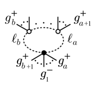
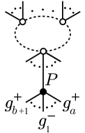
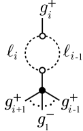
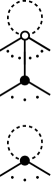
(i)                              (ii)                           (iii)                       (iv)

Figure 1: The diagrams of the one-minus rational integrand: the finite ring (i) and subtree (ii) contributions, and the divergent external bubble (iii) and tadpole diagrams (iv). The divergent diagrams are dropped and replaced by the correction term $I^{-+\cdots+}_{\rm sprs}$.

Let us now consider the integrand of the “one-minus” amplitude, $I_{n}^{-+\cdots+}$, in QCD. This amplitude vanishes in supersymmetric gauge theories so, like the all-plus amplitude, it only receives contributions from the scalar loop in the decomposition (2.1).

Naively, all the diagrams we need to consider for the one-minus integrand are given in figure 1. However, some of these diagrams are divergent, namely the external bubble diagrams in figure 1(iii) and some of the tadpoles diagrams in figure 1(iv). The tadpole contributions are harmless as argued in [12], and we will simply drop them. Our analysis below verifies that no tadpole-like correction terms need to be added to the integrand to ensure $q$-independence. The external bubble diagrams 1(iii) involve bubbles on external lines, and they are divergent because they involve an on-shell internal propagator. Thus we have to be more careful, and we now discuss the approach.

2.4.1 External bubble contributions

Unlike the all-plus integrand, the computation of the one-minus integrand faces a major obstacle: the one-minus integrand receives contributions from diagrams with an external massless bubble. These external bubble diagrams are divergent and must be “amputated”. In conventional gauges, say Feynman gauge, this amputation is straight-forward because external bubbles correspond to massless bubble integrals that integrate to zero in dimensional regularization. Amputation thus simply amounts to dropping all diagrams with bubbles on the external lines. In the CSW diagrammatic rules, however, the external bubble diagrams depicted in Figure 1(iii) contain spurious poles in the loop momentum of the form $1/\langle i|\ell_{i}|q]$, and therefore do not necessarily integrate to zero. As a consequence, naively dropping all divergent tadpole and external-bubble contributions gives a wrong integrand that contains spurious poles.

To deal with this problem, we follow a two-step strategy:

1. We first write down the naive integrand $I^{-+\cdots+}_{\rm naive}$ that is simply the sum of all finite, non-divergent diagrams contributing to the CSW expansion of the integrand. These diagrams are illustrated in Figure 1(i) and (ii). In the CSW expansion, all diagrams are finite if they contain at least two propagators of loop momenta $\ell_{i}$, $\ell_{j}$ that are non-adjacent, $j\neq i\pm 1$. Therefore, $I^{-+\cdots+}_{\rm naive}$ correctly reproduces all ($D$-dimensional) bubble cuts of two such non-adjacent loop momenta. In particular, all triangle, box and pentagon cuts are also correctly reproduced from $I^{-+\cdots+}_{\rm naive}$. However, it still contains spurious poles; these are present in cuts of two adjacent loop momenta, $\ell_{i-1}$ and $\ell_{i}$.

2. We determine a correction term $I^{-+\cdots+}_{\rm sprs}$ that satisfies two crucial properties:

   • $I^{-+\cdots+}_{\rm sprs}$ removes the spurious $q$-dependence from $I^{-+\cdots+}_{\rm naive}$, so that $I^{-+\cdots+}_{\rm naive}\!\!+I^{-+\cdots+}_{\rm sprs}$ is independent of $q$ and thus free of spurious poles.

   • $I^{-+\cdots+}_{\rm sprs}$ vanishes on any cut of two non-adjacent loop propagators; therefore, $I^{-+\cdots+}_{\rm sprs}$ can be written as a sum over terms that each contain two adjacent loop propagators, $\sim 1/{(\ell_{i-1}^{2}+\mu^{2})(\ell_{i}^{2}+\mu^{2})}$.

   $I^{-+\cdots+}_{\rm sprs}$ should be interpreted as the finite parts hidden in the divergent external-bubble diagrams of Figure 1(iii) that are needed to render the integrand $q$-independent.

Below, we will determine a $I^{-+\cdots+}_{\rm sprs}$ with these properties. We then claim that

$$I_{n}^{-+\cdots+}~{}\equiv~{}I^{-+\cdots+}_{\rm naive}+I^{-+\cdots+}_{\rm sprs}$$ (2.23)

is the correct integrand of the one-minus amplitude. Indeed, $I_{n}^{-+\cdots+}$ only contains physical poles and factorizes correctly on all $D$-dimensional bubble cuts of two loop momenta $\ell_{i}$, $\ell_{j}$ that are non-adjacent, $j\neq i\pm 1$. In the absence of spurious poles, the only remaining ambiguity are terms proportional to adjacent-line bubble and tadpole integrals; but such $D$-dimensional integrals have no scale and vanish in dimensional regularization! It follows that $I_{n}^{-+\cdots+}$ determined by the two-step strategy gives the correct one-minus amplitude.

2.4.2 Explicit all-$n$ integrand

We now carry out the two-step strategy explicitly to determine $I_{n}^{-+\cdots+}$ for any number of external legs $n$.

Step 1 is straight-forward; there are two types of finite diagrams contributing to $I_{n}^{-+\cdots+}$. The ring diagrams, which are schematically displayed in Figure 1(i), consist of a ring of vertices, all of which are UHV except for one MHV vertex containing the negative-helicity line 1. The entire contribution from ring diagrams can be combined into the following compact expression:

$$\begin{split}I^{-+\cdots+}_{\rm ring}(1,\ldots,n)~{}&=~{}2N_{p}\sum_{b>a}\frac{-\mu^{2}\langle 1\ell_{a}\rangle^{2}\langle 1\ell_{b}\rangle^{2}\langle a,a\!+\!1\rangle\langle b,b\!+\!1\rangle}{\langle 12\rangle\cdots\langle n1\rangle\langle\ell_{a}\ell_{b}\rangle\langle a\ell_{a}\rangle\langle\ell_{a},a\!+\!1\rangle\langle b,\ell_{b}\rangle\langle\ell_{b},b\!+\!1\rangle(\ell_{a}^{2}+\mu^{2})(\ell_{b}^{2}+\mu^{2})}\\ &\hskip 76.82234pt\times\langle\ell_{a}|\prod_{j=a+1}^{b-1}\biggl{[}1-\frac{\mu^{2}|\ell_{j}\rangle\langle j,j\!+\!1\rangle\langle\ell_{j}|}{(\ell_{j}^{2}+\mu^{2})\langle\ell_{j},j\rangle\langle j\!+\!1,\ell_{j}\rangle}\biggr{]}|\ell_{b}\rangle\,.\end{split}$$ (2.24)

Expanding the product over $j$ reproduces each individual ring diagram in the CSW expansion.

The second contribution comes from subtree diagrams, consisting of a ring of UHV vertices that is connected via a propagator $1/P^{2}$ to an MHV vertex that contains line 1. This contribution is illustrated in Figure 1(ii). The computation of the “ring” part of these diagrams coincides with our analysis for the all-plus integrand $I^{++\cdots+}$ in section 2.3. We find,

$$\begin{split}I^{-+\cdots+}_{\rm subtree}(1,\ldots,n)=&\sum_{2\leq b-a\leq n-2}\frac{\langle 1P\rangle^{4}}{\langle P,b\!+\!1\rangle\langle b\!+\!1,b\!+\!2\rangle\cdots\langle a\!-\!1,a\rangle\langle aP\rangle}\times\frac{1}{P^{2}}\times I_{\rm CSW}^{++\cdots+}(a\!+\!1,\ldots,b,P)\,.\end{split}$$ (2.25)

where

$$P\equiv p_{a+1}+p_{a+2}+\dots+p_{b}\,.$$ (2.26)

The range of $a$ and $b$ in the sum is chosen such that $a$ and $b$ are non-adjacent. As $P$ is an off-shell momentum, the CSW prescription is understood for all occurrences of $|P\rangle$ in the CSW all-plus integrand $I_{\rm CSW}^{++\cdots+}$, defined in (2.14). The naive integrand is the sum of the ring and subtree contributions,

$$I^{-+\cdots+}_{\rm naive}~{}=~{}I^{-+\cdots+}_{\rm ring}+I^{-+\cdots+}_{\rm subtree}\,.$$ (2.27)

As it stands, the integrand $I^{-+\cdots+}_{\rm naive}$ factorizes correctly on $D$-dimensional pentagon, box, triangle, and non-adjacent bubble cuts. However, it contains uncanceled spurious singularities of the form $1/\langle i\ell_{i}\rangle^{2}$ and $1/(\langle i-1,\ell_{i-1}\rangle\langle i\,\ell_{i}\rangle)$ with $i=2,\ldots,n$ , where the $|\ell_{i}\rangle$ depend on the reference $q$ through the CSW prescription (2.4). This is not surprising, considering that we have dropped the (divergent) external bubble contributions displayed in Figure 1(iii) that contain such spurious singularities.

We now proceed with step 2 of the above strategy, and try to determine a correction term $I^{-+\cdots+}_{\rm sprs}$ that cancels the spurious $q$-dependence in $I^{-+\cdots+}_{\rm naive}$ without spoiling its crucial factorization properties. We make the ansatz

$$I^{-+\cdots+}_{\rm sprs}~{}=~{}2N_{p}\sum_{i=2}^{n}\frac{\mu^{2}}{\langle 12\rangle\cdots\langle n1\rangle(\ell_{i-1}^{2}+\mu^{2})(\ell_{i}^{2}+\mu^{2})}\Biggl{(}\frac{D_{i}}{\langle i\ell_{i}\rangle^{2}}+\frac{S_{i}}{\langle i\ell_{i}\rangle}\Biggr{)}\,,$$ (2.28)

where the residues of the double and single spurious poles in $\langle i\ell_{i}\rangle\!=\!\langle i|\ell_{i}|q]$ are controlled by the kinematic coefficients $D_{i}$ and $S_{i}$. These coefficients are highly constrained by little-group properties and are not allowed to contain any $\ell$-dependent denominator factors. A numeric analysis gives the following solution:

$$D_{i}~{}=\,-\langle 1i\rangle^{2}\langle 1\ell_{i-1}\rangle\langle 1\ell_{i}\rangle\,,~{}\qquad S_{i}~{}=~{}\langle 1i\rangle^{2}\biggl{[}\frac{\langle 1,i-1\rangle\langle 1\ell_{i}\rangle}{\langle i-1,i\rangle}-\frac{\langle 1,i+1\rangle\langle 1\ell_{i-1}\rangle}{\langle i,i+1\rangle}\biggr{]}\,.$$ (2.29)

While not obvious, $I^{-+\cdots+}_{\rm sprs}$ indeed cancels all spurious poles in the naive integrand, rendering it $q$-independent. In summary, the $n$-point one-minus integrand is given by

$$\boxed{\begin{split}&I_{n}^{-+\cdots+}~{}=~{}I^{-+\cdots+}_{\rm ring}+I^{-+\cdots+}_{\rm subtree}+I^{-+\cdots+}_{\rm sprs}\phantom{\biggl{(}}\\ &=~{}\!\!\!\sum_{b>a}\frac{-2N_{p}\,\mu^{2}\langle 1\ell_{a}\rangle^{2}\langle 1\ell_{b}\rangle^{2}\langle a,a\!+\!1\rangle\langle b,b\!+\!1\rangle}{\langle 12\rangle\cdots\langle n1\rangle\langle\ell_{a}\ell_{b}\rangle\langle a\ell_{a}\rangle\langle\ell_{a},a\!+\!1\rangle\langle b,\ell_{b}\rangle\langle\ell_{b},b\!+\!1\rangle(\ell_{a}^{2}+\mu^{2})(\ell_{b}^{2}+\mu^{2})}\\ &\hskip 76.82234pt\times\langle\ell_{a}|\prod_{j=a+1}^{b-1}\biggl{[}1-\frac{\mu^{2}|\ell_{j}\rangle\langle j,j\!+\!1\rangle\langle\ell_{j}|}{(\ell_{j}^{2}+\mu^{2})\langle\ell_{j},j\rangle\langle j\!+\!1,\ell_{j}\rangle}\biggr{]}|\ell_{b}\rangle\\ &~{}~{}~{}~{}+\sum_{2\leq b-a\leq n-2}\frac{\langle 1P\rangle^{4}}{\langle P,b\!+\!1\rangle\langle b\!+\!1,b\!+\!2\rangle\cdots\langle a\!-\!1,a\rangle\langle aP\rangle}\times\frac{1}{P^{2}}\times I_{\rm CSW}^{++\cdots+}(a\!+\!1,\ldots,b,P)\\ &~{}~{}~{}~{}+\sum_{i=2}^{n}\frac{-2N_{p}\,\mu^{2}\langle 1i\rangle^{2}}{\langle 12\rangle\cdots\langle n1\rangle(\ell_{i}^{2}\!+\!\mu^{2})(\ell_{i\text{-}1}^{2}\!+\!\mu^{2})\langle i\,\ell_{i}\rangle}\times\Biggl{[}\frac{\langle 1\ell_{i\text{-}1}\rangle\langle 1\ell_{i}\rangle}{\langle i\ell_{i}\rangle}\!-\!\frac{\langle 1,i\!-\!1\rangle\langle 1\ell_{i}\rangle}{\langle i\!-\!1,i\rangle}\!+\!\frac{\langle 1,i\!+\!1\rangle\langle 1\ell_{i\text{-}1}\rangle}{\langle i,i\!+\!1\rangle}\Biggr{]}\,.\end{split}}$$ (2.30)

We have performed various checks on the correctness of the integrand (2.30). Specifically, we have numerically verified $q$ independence of the integrand for $n=4,5,6,7,8,9,10$. For $n=4$, we have gone further and explicitly re-expressed the integrand $I_{4}^{-+++}$ in a manifestly $q$-independent form. We have then performed integral reduction on this form and matched it to the result of Bern and Morgan [23],

$$\begin{split}&A_{4}^{\rm QCD}(1^{-},\,2^{+},3^{+},4^{+})\\ &={2iN_{p}\over(4\pi)^{2-\epsilon}}{[24]^{2}\over[12]\langle 23\rangle\langle 34\rangle[41]}\frac{st}{u}\biggl{[}\frac{t(u\,\text{-}\,s)}{su}J_{3}(s)+\frac{s(u\,\text{-}\,t)}{tu}J_{3}(t)-{t\,\text{-}\,u\over s^{2}}J_{2}(s)-{s\,\text{-}\,u\over t^{2}}J_{2}(t)+{st\over 2u}J_{4}+K_{4}\biggr{]}\,.\end{split}$$ (2.31)

Here, $K_{4}$ is a box integral in $D=8-2\epsilon$ dimensions, while $J_{2}$, $J_{3}$ and $J_{4}$ are bubble, triangle and box integrals in $D=6-2\epsilon$ dimensions (see [23] for a precise definition). To match $I_{4}^{-+++}$ to the integrand in (LABEL:bm), we dropped terms that integrate to zero.

3 CSW expansion for Coulomb-branch amplitudes in ${\cal N}=4$ SYM

In this section, we derive the massive CSW expansion for Coulomb-branch amplitudes in ${\cal N}=4$ SYM that was proposed in [18]. We first briefly review ${\cal N}=4$ SYM theory on the Coulomb branch and the proposed CSW expansion. We then examine the supersymmetric properties of the massive CSW rules. Finally, we present a proof of the expansion.

3.1 Review: ${\cal N}=4$ SYM on the Coulomb branch and its massive CSW expansion

We consider ${\cal N}\!=\!4$ SYM with gauge group $U(M\!+\!N)$. The simplest way to move onto the Coulomb-branch is to give vevs to a subset of the scalars,

$$\big{\langle}(\phi_{12})_{A}{}^{B}\big{\rangle}\,=\,\big{\langle}(\phi_{34})_{A}{}^{B}\big{\rangle}\,=\,m\,\delta_{A}{}^{B}\qquad\qquad\text{ for }~{}~{}~{}1\leq A,B\leq M\,.$$ (3.1)

Here and in the following we suppress all coupling dependence, effectively setting $g=1$. These vevs break the gauge group spontaneously to $U(M)\!\times\!U(N)$, and the $R$-symmetry group as $SU(4)\rightarrow Sp(4)$. They also split the states into a massless and a massive sector. The massless sector contains the gluons $g^{\pm}$, fermions $\chi^{a}$, and scalars $\phi^{ab}$, where $a,b$ are R-symmetry indices. The massive sector contains fields of mass $m$ that are bifundamental with respect to $U(M)\!\times\!U(N)$, consisting of $W$ bosons, scalars $w$, and fermions $\Psi$. The conjugate particles in the bifundamental of $U(N)\!\times\!U(M)$ have mass parameter $-m$. Table 1 summarizes the massless and massive states, their polarizations and wave functions, and how they correspond to each other.

	massless fields	massive fields	wave functions
gluons / $W^{\pm}$-boson:	$g^{+}$, $g^{-}$	$W^{+}$, $W^{-}$	$\epsilon_{-}\!=\!\frac{\sqrt{2}|i^{\perp}\rangle[q|}{[i^{\perp}q]},~{}\epsilon_{+}\!=\!\frac{\sqrt{2}|q\rangle[i^{\perp}|}{\langle i^{\perp}q\rangle}$
scalar / $W^{L}$-boson:	$\tfrac{1}{\sqrt{2}}(\phi^{12}\!+\!\phi^{34})$	$W^{L}\!\sim\!\tfrac{1}{\sqrt{2}}(w^{12}\!+\!w^{34})$	$\not{\epsilon}_{L}=\frac{1}{m_{i}}\Big{(}\not{p}_{i}^{\perp}+\frac{m_{i}^{2}}{2q\cdot p_{i}}\not{q}\Big{)}$
scalars:	$\phi^{13}$​, $\phi^{14}$​, $\phi^{23}$​, $\phi^{24}$​,	$w^{13}$, $w^{14}$, $w^{23}$, $w^{24}$,
	$\tfrac{1}{\sqrt{2}}(\phi^{12}\!-\!\phi^{34})$	$\tfrac{1}{\sqrt{2}}(w^{12}\!-\!w^{34})$
fermions:	$\chi^{a}$, $\chi^{abc}$	$\Psi^{a}$	$v_{+}\!=\!\begin{pmatrix}\!|p^{\perp}]\\[2.84526pt] \!\frac{im|q\rangle}{\langle qp^{\perp}\rangle}\end{pmatrix},~{}v_{-}\!=\!\begin{pmatrix}\!\frac{im|q]}{[p^{\perp}q]}\\[2.84526pt] \!|p^{\perp}\rangle\end{pmatrix}$

Table 1: Massless and massive particles on the Coulomb branch for the R-symmetry breaking $SU(4)\!\rightarrow\!Sp(4)$. The massive fermions $\Psi^{a}$ are 4-component Dirac fermions.

The Coulomb branch of ${\cal N}=4$ SYM can be interpreted as arising from dimensional reduction of massless ${\cal N}=(1,1)$ SYM in 6 dimensions. In this interpretation, the mass parameters $m_{i}$ of particles are related to momenta in the extra dimensions, $m_{i}=p_{5}+ip_{6}$. The external particles of any non-vanishing Coulomb-branch amplitude must satisfy

$$\sum_{i}m_{i}~{}=~{}0\,.$$ (3.2)

For simplicity, we will take the $m_{i}$ to be real (but either +ve or -ve) in the following and refer to them as “masses”.

The massive spinor-helicity formalism
A convenient way to express amplitudes on the Coulomb-branch of ${\cal N}=4$ SYM is the massive spinor-helicity formalism [53, 54]. One decomposes a massive on-shell momentum $p_{i}$ of mass $m_{i}$ in terms of a pair of null vectors, a reference null $q$ and the null projection $p_{i}^{\perp}$, viz.

$$p_{i}=p_{i}^{\perp}-\frac{m_{i}^{2}}{2q\cdot p_{i}}\,q\,,\qquad\quad p_{i}^{2}=-m_{i}^{2}\,.$$ (3.3)

Since $p_{i}^{\perp}$ and $q$ are null vectors, there are associated spinors $|i^{\perp}\rangle,|i^{\perp}],~{}|q\rangle,|q]$, such that

$$(p_{i}^{\perp})^{\dot{\alpha}\alpha}~{}=~{}|i^{\perp}\rangle^{\dot{\alpha}}[i^{\perp}|^{\alpha}\,,\qquad q^{\dot{\alpha}\alpha}~{}=~{}|q\rangle^{\dot{\alpha}}[q|^{\alpha}\,.$$ (3.4)

For massive vector bosons, the spinors $|q\rangle$ and $|q]$ allow us to define a convenient basis of polarization vectors:

$$\epsilon_{-}=\frac{\sqrt{2}|i^{\perp}\rangle[q|}{[i^{\perp}q]}~{}~{}\,,~{}\qquad\epsilon_{+}=\frac{\sqrt{2}|q\rangle[i^{\perp}|}{\langle i^{\perp}q\rangle}~{}~{}\,,~{}\qquad\not{\epsilon}_{0} = \frac{1}{m_{i}}\Big{(}\not{p}_{i}^{\perp}-\frac{m_{i}^{2}}{\langle q|p_{i}|q]}\not{q}\Big{)}\,.$$ (3.5)

In the following we will denote this basis of polarization vectors as “$q$-helicity basis”. For example, vector bosons with polarizations $\epsilon_{\pm}$ and $\epsilon_{0}$ have $q$-helicity $h=\pm 1$ and $h=0$, respectively. It is convenient to use the spinor $|q]$ also as the reference spinor in the CSW expansion.

MHV-classification
The familiar N^kMHV classification of massless $\mathcal{N}=4$ SYM amplitudes has to be augmented when applied to Coulomb branch amplitudes. Each of the two $SU(2)$-sectors of the unbroken $Sp(4)$ R-symmetry has an N^kMHV classification with non-vanishing amplitudes for $k=-1$ (ultra-helicity violating, UHV), $k=0$ (MHV), $k=1$ (NMHV) etc. Thus we classify the massive Coulomb-branch amplitudes as UHV$\times$UHV, UHV$\times$MHV, MHV$\times$MHV etc. When no confusion is possible, we will refer to UHV$\times$UHV and MHV$\times$MHV as the UHV and MHV sectors, respectively.

Soft-limit construction of massive amplitudes from massless amplitudes
In [17, 18], it was proposed that massive Coulomb-branch on-shell amplitudes can be expressed in terms of massless amplitudes at the origin of moduli space. Non-trivial evidence for this proposal was presented in [17] at leading order, and in [18] to all orders. We now review the details of this proposal, for the special case of Coulomb-branch tree-level scattering of two adjacent massive $W$-bosons $W_{1}$, $W_{2}$ with an arbitrary number of additional massless particles. Such an amplitude can be expressed in terms of massless ${\cal N}=4$ amplitudes as

$$\bigl{\langle}\,W_{1}{\overline{W\!}\,}_{2}\,\ldots\,\bigr{\rangle}~{}~{}=~{}~{}\lim_{\varepsilon\rightarrow 0}\,\sum_{s=0}^{\infty}\,\,\bigl{\langle}\,g_{1}\,\underbrace{\phi^{\rm vev}_{\varepsilon q}\!.\,.\,\phi^{\rm vev}_{\varepsilon q}}_{s\text{ times}}\,g_{2}\,\ldots\,\bigr{\rangle}_{\rm sym}\,,$$ (3.6)

where the $\ldots$ represent arbitrary further massless particles in the amplitude. Some elaborations on the proposal (3.6) are in order:

• The polarizations of the $W$-bosons on the left-hand side are chosen in the $q$-helicity basis (3.5). The massless gluons $g_{1}$, $g_{2}$ have the corresponding massless helicity.

• The massless gluons $g_{1}$, $g_{2}$ on the right-hand side have momenta $p_{i}^{\perp}$ that are related to the massive momenta of the $W$-bosons via (3.3).

• The reference vector $q$ is subject to the constraint

  $$\sum_{i=1}^{n}\frac{m_{i}^{2}}{2\,q\!\cdot\!p_{i}}~{}=~{}0\,,$$ (3.7)

  which ensures momentum conservation on the right-hand side, $\sum_{i}p_{i}^{\perp}=0$. For the two-mass case at hand, (3.7) is equivalent to the simple orthogonality condition $q\cdot(p_{1}+p_{2})=0$ .

• The scalar $\phi^{\rm vev}_{\varepsilon q_{i}}$ is a massless soft scalar of momentum $\varepsilon q_{i}$ whose R-symmetry structure is oriented in the Coulomb-branch vev direction, $\phi^{\rm vev}=\langle\phi_{ab}\rangle\phi^{ab}$. In our case, we thus have

  $$\phi^{\rm vev}~{}=~{}m\bigl{(}\phi^{12}+\phi^{34}\bigr{)}\,.$$ (3.8)

• The subscript ‘sym’ denotes a symmetrization of the vev scalars in their momenta $q_{i}$ before taking the collinear limit $q_{i}\rightarrow q$. This sum over permutations ensures that they are “unordered” particles in the massless partial amplitudes, which befits a vev scalar that must live in the Cartan subalgebra and thus commute with itself. The symmetrization ensures that the the right-hand side of (3.6) is finite in the collinear limit $q_{i}\rightarrow q$.

It was shown in [18], that the multi-soft limit in (3.6) is well-defined, i.e. it is free of collinear and soft divergences. It was also shown that the proposal (3.6), and its generalization to amplitudes and loop integrands with arbitrarily many massive particles, implies a massive CSW vertex expansion, which we now review.

Massive CSW rules
In [18], it was shown that the soft-limit construction detailed above is equivalent to a massive CSW expansion for Coulomb-branch amplitudes in the $q$-helicity basis. We now review the diagrammatic rules of this expansion.

The propagators in the massive CSW expansion are conventional massive scalar propagators:

$$\parbox[c]{51.21504pt}{\includegraphics[width=45.52458pt]{propm2}}~{}=~{}\frac{1}{P_{I}^{2}+m_{I}^{2}}\,.$$ (3.9)

Just like momentum is conserved at each vertex, the mass parameters $m_{i}$ also sum to zero at each vertex; therefore, the internal mass $m_{I}$ is given by the sum of masses of the other lines at the left or right vertex. Of course, (3.9) includes massless propagators as a special case when $m_{I}\!=\!0$.

There are three types of vertices in the expansion:

• The first vertex is the conventional MHV vertex, with perp’ed spinors:

  $$\parbox[c]{62.59596pt}{\includegraphics[width=42.67912pt]{cswnptgen}}~{}=~{}\frac{\delta^{(8)}\big{(}|i^{\perp}\rangle\eta_{ia}\big{)}}{\langle 1^{\perp}2^{\perp}\rangle\cdots\langle n^{\perp}1^{\perp}\rangle}\,.$$ (3.10)

• The second vertex is an ultra-helicity-violating (UHV) vertex:

  $$\parbox[c]{48.36958pt}{\includegraphics[width=42.67912pt]{cswnpt2softgen}}~{}=~{}K_{n}^{2}\times\frac{\delta^{(4)}\big{(}\langle qi^{\perp}\rangle\eta_{ia}\big{)}}{\langle 1^{\perp}2^{\perp}\rangle\cdots\langle n^{\perp}1^{\perp}\rangle}\,.$$ (3.11)

  The kinematic prefactor $K_{n}$ is given by

  $$K_{n}~{}=~{}\sum_{i}\frac{m_{i}\langle Xi^{\perp}\rangle}{\langle Xq\rangle\langle i^{\perp}q\rangle}\,,$$ (3.12)

  for arbitrary reference spinor $|X\rangle\neq|q\rangle$. In fact, using $\sum_{i}m_{i}=0$ it is easy to see that $K_{n}$ is independent of the choice of $|X\rangle$ [18]. The vertex (3.11) is $O(m^{2})$ and thus not present for massless amplitudes.

  The vertex (3.11) generalizes the UHV vertices (2.8) that we encountered in the scalar-vector theory; in fact, a short computation shows that, with $m\equiv m_{1}=-m_{2}$ and $m_{i}=0$ for $i\geq 3$, we can reproduce the vertex (2.8) by projecting out a pair of conjugate scalars on lines $1$ and $2$:

  $$\frac{\partial^{2}}{\partial\eta_{11}\partial\eta_{12}}\,\frac{\partial^{2}}{\partial\eta_{23}\partial\eta_{24}}\,\,\frac{K_{n}^{2}\,\delta^{(4)}\big{(}\langle qi^{\perp}\rangle\eta_{ia}\big{)}}{\langle 1^{\perp}2^{\perp}\rangle\cdots\langle n^{\perp}1^{\perp}\rangle}~{}=~{}\frac{m^{2}\langle 12\rangle}{\langle 23\rangle\cdots\langle n1\rangle}\,.$$ (3.13)

  In particular, all dependence on the holomorphic reference spinor $|q\rangle$ cancels in this case.

• Finally, there is a third vertex, which breaks the R-symmetry $SU(4)\rightarrow Sp(4)$. This “MHV$\times$UHV vertex” has the structure of the MHV vertex (3.10) with respect to one of the two $SU(2)$ factors in $Sp(4)$, and the structure of the UHV vertex (3.11) with respect to the other $SU(2)$. Explicitly,

  $$\parbox[c]{48.36958pt}{\includegraphics[width=42.67912pt]{cswnpt1softgen}}~{}=~{}K_{n}\times\frac{\delta^{(4)}_{12}\big{(}|i^{\perp}\rangle\eta_{ia}\big{)}\,\delta^{(2)}_{34}\big{(}\langle qi^{\perp}\rangle\eta_{ia}\big{)}+\delta^{(4)}_{34}\big{(}|i^{\perp}\rangle\eta_{ia}\big{)}\,\delta^{(2)}_{12}\big{(}\langle qi^{\perp}\rangle\eta_{ia}\big{)}}{\langle 1^{\perp}2^{\perp}\rangle\cdots\langle n^{\perp}1^{\perp}\rangle}\,,$$ (3.14)

  where $K_{n}$ is given by (3.12). The subscripts on the Grassmann $\delta$-functions indicate which of the two $SU(2)$ factors of $Sp(4)$ the $\delta$-function ‘lives in’.

An example for an amplitude computed from these rules is the scattering of two $W$ bosons of mass $m$ with arbitrarily many massless gluons $g$,

$$\bigl{\langle}W_{1}^{-}{\overline{W\!}\,}_{2}^{+}\,g_{3}^{+}\ldots g_{n}^{+}\bigl{\rangle}~{}=~{}-\frac{m^{2}\langle q1^{\perp}\rangle^{2}}{\langle q2^{\perp}\rangle^{2}\langle 2^{\perp}3\rangle\langle 34\rangle\cdots\langle n1^{\perp}\rangle}\times\big{\langle}2^{\perp}\big{|}\prod_{j=3}^{n-1}\biggl{[}1-\frac{m^{2}|P_{J}\rangle\langle j,j\!+\!1\rangle\langle P_{J}|}{(P_{J}^{2}+m^{2})\langle P_{J},j\rangle\langle j\!+\!1,P_{J}\rangle}\biggr{]}\big{|}1^{\perp}\big{\rangle}\,,$$ (3.15)

where we denoted $P_{J}\equiv P_{2..j}$. This amplitude is related by supersymmetry to the massive-scalar amplitude (2.13). In fact, these two amplitude only differ by the spinor factor $\langle q1^{\perp}\rangle^{2}/\langle q2^{\perp}\rangle^{2}$, which corrects the helicity weights. The amplitude (3.15) has only one negative-helicity particle and is thus in the UHV sector. UHV amplitudes vanish in the massless limit due to supersymmetry. The UHV sector is the “lowest” non-vanishing sector on the Coulomb branch. Indeed, unlike in non-supersymmetric theories, the all-plus amplitude vanishes in ${\cal N}=4$ SYM even on the Coulomb branch. This follows directly from SUSY Ward identities [15].

For $q$’s satisfying (3.7), it was shown in [18] that this massive CSW expansion is identical to the soft-limit construction (3.6). In section 3.4, we will present a recursion relation derivation of this expansion that is in fact valid for any choice of reference vector $q$.

3.2 Manifest $\tilde{Q}$-supersymmetry of massive CSW rules

The CSW rules in massless ${\cal N}=4$ SYM  manifestly preserve the $\tilde{Q}$ supercharges, diagram by diagram. In fact, MHV vertices contain an overall factor of $\delta^{(8)}(|\tilde{Q}\rangle)$, where $|\tilde{Q}_{a}\rangle$ are the holomorphic supercharges in the massless case, $|\tilde{Q}_{a}\rangle=\sum_{i}|i\rangle\eta_{ia}$. On the Coulomb branch, these supercharges are deformed because the super-algebra acquires a central charge:

$$|\tilde{Q}_{a}\rangle\,=\,\sum_{i}|\tilde{Q}_{ia}\rangle\,,\qquad\text{ with }~{}~{}~{}~{}|\tilde{Q}_{ia}\rangle\,=\,|i^{\perp}\rangle\eta_{ia}-\frac{m_{i}|q\rangle}{\langle qi^{\perp}\rangle}\Omega_{ab}\frac{\partial}{\partial\eta_{ib}}\,,\quad\Omega_{ab}~{}=~{}\begin{pmatrix}i\sigma_{2}&0\\ 0&i\sigma_{2}\end{pmatrix}\,.$$ (3.16)

For example,

$$|\tilde{Q}_{i1}\rangle\,=\,|i^{\perp}\rangle\eta_{i1}-\frac{m_{i}|q\rangle}{\langle qi^{\perp}\rangle}\frac{\partial}{\partial\eta_{i2}}\,.$$ (3.17)

Each vertex in the massive CSW expansion, (3.10), (3.11), and (3.14), is individually invariant only under half of the $\tilde{Q}$ SUSY charges, namely under the $q$-projection of $|\tilde{Q}_{a}\rangle$,

$$\langle q\tilde{Q}_{a}\rangle=\sum_{i}\langle qi^{\perp}\rangle\eta_{ia}\,.$$ (3.18)

They cannot be individually invariant under the entire $|\tilde{Q}_{a}\rangle$-symmetry, because the full generators (3.16) mix different $\eta$ degrees. It is therefore convenient to combine vertices of different $\eta$-degree into a supervertex,

$$\begin{split}\parbox[c]{42.67912pt}{\includegraphics[width=42.67912pt]{cswnptsupergen}}~{}&\equiv~{}\parbox[c]{42.67912pt}{\includegraphics[width=42.67912pt]{cswnpt2softgen}}+\parbox[c]{42.67912pt}{\includegraphics[width=42.67912pt]{cswnpt1softgen}}+\parbox[c]{42.67912pt}{\includegraphics[width=42.67912pt]{cswnptgen}}~{}=~{}\frac{{\cal V}_{n}}{\langle 1^{\perp}2^{\perp}\rangle\cdots\langle n^{\perp}1^{\perp}\rangle}\,,\end{split}$$ (3.19)

with

$${\cal V}_{n}~{}=~{}\Bigl{[}\delta^{(4)}_{12}\big{(}|i^{\perp}\rangle\eta_{ia}\big{)}+K_{n}\delta^{(2)}_{12}\big{(}\langle qi^{\perp}\rangle\eta_{ia}\big{)}\Bigr{]}\Bigl{[}\delta^{(4)}_{34}\big{(}|i^{\perp}\rangle\eta_{ia}\big{)}+K_{n}\delta^{(2)}_{34}\big{(}\langle qi^{\perp}\rangle\eta_{ia}\big{)}\Bigr{]}\,.$$ (3.20)

This supervertex, just as the massless MHV vertex, preserves all $\tilde{Q}$ supersymmetries. Indeed,

$$|\tilde{Q}_{a}\rangle{\cal V}_{n}~{}=~{}0\,,\qquad\text{with }~{}~{}|\tilde{Q}_{a}\rangle\equiv\sum_{i}|\tilde{Q}_{ia}\rangle\,.$$ (3.21)

In fact, ${\cal V}_{n}$ is nothing but the product of the $\tilde{Q}$ supercharges:

$${\cal V}_{n}~{}=~{}\delta^{(8)}\Bigl{(}|\tilde{Q}_{a}\rangle\Bigr{)}~{}=~{}\frac{1}{2^{4}}\prod_{a=1}^{4}\sum_{i,j}\langle Q_{ia}\,Q_{ja}\rangle\,.$$ (3.22)

In this expression, all $\eta$-derivatives need to be carried out, so that ${\cal V}_{n}$ is a Grassmann polynomial with kinematic coefficients, and not a Grassmann differential operator. Note that the $\delta$-function is indeed well-defined despite the $\eta$-derivatives in the definition of the $\tilde{Q}_{a}$ supercharges, because these anticommute with each other:

$$\bigl{\{}|\tilde{Q}_{a}\rangle,|\tilde{Q}_{b}\rangle\bigr{\}}~{}=~{}0\,.$$ (3.23)

This follows from the SUSY algebra

$$\bigl{\{}|\tilde{Q}_{ia}\rangle^{\dot{\alpha}},|\tilde{Q}_{jb}\rangle^{\dot{\beta}}\bigr{\}}~{}=~{}-m_{i}\,\delta_{ij}\epsilon^{\dot{\alpha}\dot{\beta}}\,\Omega_{ab}\,,$$ (3.24)

together with $\sum_{i}m_{i}=0$. Crucially, it does not rely on the lines $i$ being on-shell, and thus also holds for CSW vertices with off-shell internal lines, whose angle spinors are given by the CSW prescription (2.4).

It is easy to verify explicitly that (3.22) is equivalent to (3.20). For example,

$$\begin{split}\delta^{(2)}(\tilde{Q}_{1})\delta^{(2)}(\tilde{Q}_{2})~{}&=~{}\delta^{(2)}\biggl{(}|i^{\perp}\rangle\eta_{i1}-\frac{m_{i}|q\rangle}{\langle qi^{\perp}\rangle}\frac{\partial}{\partial\eta_{i2}}\biggr{)}\delta^{(2)}\bigl{(}|j^{\perp}\rangle\eta_{j2}\bigr{)}\\ ~{}&=~{}\frac{\delta^{(2)}_{12}\bigl{(}\langle qi^{\perp}\rangle\eta_{ia}\bigr{)}}{\langle qX\rangle^{2}}\biggl{(}\langle Xi^{\perp}\rangle\eta_{i1}-\frac{m_{i}\langle Xq\rangle}{\langle qi^{\perp}\rangle}\frac{\partial}{\partial\eta_{i2}}\biggr{)}\Bigl{(}\langle Xj^{\perp}\rangle\eta_{j2}\Bigr{)}\\[4.30554pt] ~{}&=~{}\delta_{12}^{(4)}\bigl{(}|i^{\perp}\rangle\eta_{ia}\bigr{)}+K_{n}\,\delta_{12}^{(2)}\bigl{(}\langle qi^{\perp}\rangle\eta_{ia}\bigr{)}\,,\end{split}$$ (3.25)

and similarly in the other $SU(2)$ sector.

Expressed in terms of supercharges, the massive CSW supervertex thus takes the same form as in the massless case,

$$\boxed{~{}~{}\parbox[c]{42.67912pt}{\includegraphics[width=42.67912pt]{cswnptsupergen}}~{}\equiv~{}\frac{\delta^{(8)}\Bigl{(}|\tilde{Q}_{a}\rangle\Bigr{)}}{\langle 1^{\perp}2^{\perp}\rangle\cdots\langle n^{\perp}1^{\perp}\rangle}\,.~{}~{}~{}}$$ (3.26)

This form of the supervertex turns out to be convenient for our loop-level derivation of the CSW rules.

The form (3.26) of the supervertex also allows a convenient new representation of products of supervertices. For example, one can rewrite subdiagrams with two vertices that are connected by $M$ internal lines $P_{I}$ in the following way:

$$\begin{split}\parbox[c]{85.35826pt}{\includegraphics[width=85.35826pt]{LR2vertices}}~{}&\propto~{}\int d^{4M}\eta_{P_{I}a}\,{\cal V}_{L,P_{I}}\,{\cal V}_{R,\text{-}P_{I}}\\[-12.91663pt] ~{}&=~{}\int d^{4M}\eta_{P_{I}a}\,\biggl{[}\delta^{(8)}\biggl{(}\,\sum_{i\in L,P_{I}}\!\!|\tilde{Q}_{ia}\rangle\biggr{)}\biggr{]}\biggl{[}\delta^{(8)}\biggl{(}\,\sum_{i\in R,\text{-}P_{I}}\!\!|\tilde{Q}_{ia}\rangle\biggr{)}\biggr{]}\\[4.30554pt] ~{}&=~{}\delta^{(8)}\biggl{(}\,\sum_{i\in L,R}\!\!|\tilde{Q}_{ia}\rangle\biggr{)}\,\int d^{4M}\eta_{P_{I}a}\,\delta^{(8)}\biggl{(}\,\sum_{i\in R,\text{-}P_{I}}\!\!|\tilde{Q}_{ia}\rangle\biggr{)}\,.\end{split}$$ (3.27)

In the sums, we denoted the lines on the left and right vertex that do not directly connect the two vertices by $L$ and $R$, respectively. In the final expression, the $\eta$-differentiations act throughout the expression; for example the differentiations in the left $\delta$-function can also act on the right $\delta$-function. This is to be contrasted with the definition of ${\cal V}_{n}$, (3.22), where all differentiations are carried out within the $\delta$-function. In particular, the overall $\delta$-function in (3.27) cannot be simply replaced by a factor of ${\cal V}_{L,R}$! While trivial in the massless case, the identity (3.27) on the Coulomb branch takes some tedious but straight-forward algebra to derive. Iterating this identity, it is clear that we can pull an “overall” $\delta$-function out of any diagram. Specifically, any diagram with $M$ internal lines $P_{I}$ can be brought into the form

$$\parbox[c]{56.9055pt}{\includegraphics[width=56.9055pt]{allminusdiag}}~{}=~{}\delta^{(8)}\biggl{(}\sum_{i=1}^{n}|\tilde{Q}_{ia}\rangle\biggr{)}\int d^{4M}\eta_{P_{I}}\bigl{[}\ldots\bigr{]}\,.$$ (3.28)

On the left-hand side, the striped blob denotes any individual supervertex diagram that contributes to the $n$-point amplitude. Again, we do not need to impose on-shell conditions on the external lines $i$, and all differentiations in the $|\tilde{Q}_{ia}\rangle$ act also on the remaining $\eta$-dependence in the ‘$\ldots$’. This representation makes the $\tilde{Q}$-supersymmetry of each individual massive CSW diagram completely manifest.

3.3 Manifest $Q$-supersymmetry of massive CSW rules

The massive CSW rules do not only preserve all $\tilde{Q}$ supersymmetries, they also preserve half of the $Q$ supersymmetries, diagram by diagram, even off-shell. Indeed, by momentum conservation each vertex of each diagram is invariant under the collective shift of all $\eta$-variables,

$$\eta_{ia}~{}\rightarrow~{}\eta_{ia}+[qi^{\perp}]\delta\eta_{a}\,,$$ (3.29)

which is generated by the supercharge

$$[q\,Q^{a}]~{}=~{}\sum_{i}[qi^{\perp}]\frac{\partial}{\partial\eta_{ia}}\,.$$ (3.30)

One consequence of manifest $[q\,Q^{a}]$ supersymmetry is that all-minus amplitudes and integrands vanish diagram by diagram, even off shell:

$$\parbox[c]{56.9055pt}{\includegraphics[width=56.9055pt]{allminus}}~{}=~{}0\,.$$ (3.31)

This is not surprising, because $[q\,Q^{a}]$ Ward identities can be used to show that massive all-minus amplitudes vanish [56]. Technically, the reason for (3.31) is that a full fermionic integral over an integrand with a fermionic “zero mode” vanishes. Indeed,

$$\begin{split}\parbox[c]{56.9055pt}{\includegraphics[width=56.9055pt]{allminus}}~{}&=~{}\int d^{4}\eta_{1a}d^{4}\eta_{2a}\cdots d^{4}\eta_{na}\,\parbox[c]{56.9055pt}{\includegraphics[width=56.9055pt]{allminusdiag}}\\[-12.91663pt] ~{}&=~{}\frac{1}{[q1^{\perp}]^{4}}\int d^{4}\eta_{2a}\cdots d^{4}\eta_{na}\,\prod_{b}[q\,Q^{b}]\parbox[c]{56.9055pt}{\includegraphics[width=56.9055pt]{allminusdiag}}\\[-4.30554pt] ~{}&=~{}0\,.\end{split}$$ (3.32)

The manipulation from the 1st line to the 2nd line is valid because $\eta$-integrals of all lines $i=1,\dots,n$ are present.

3.4 Derivation of the expansion: tree amplitudes

To derive the massive CSW expansion for Coulomb-branch amplitudes, we make use of on-shell recursion relations. On-shell recursion relations are based on a complex shift $p_{i}\rightarrow\hat{p}_{i}(z)$ of the external momenta of an on-shell amplitude. The complex shift must preserve the on-shell condition, $\hat{p}_{i}^{2}=m_{i}^{2}$, and momentum conservation, $\sum_{i}\hat{p}_{i}=0$. Analytic properties of the $z$-dependent on-shell amplitude $\hat{A}_{n}(z)$ can then be used to express the amplitude in terms of its factorization channels, which involve products of two lower-point on-shell amplitudes. On-shell recursion relations are straight-forwardly applicable when the amplitude vanishes at large $z$, $\hat{A}_{n}(z)\rightarrow 0$. In that case factorization channels completely determine the amplitude. If $\hat{A}_{n}(z)$ does not vanish as $z\rightarrow\infty$, there is an additional “boundary” contribution to the recursion relation from the residue picked up by a contour around $z=\infty$,

$$B_{n}~{}\equiv~{}\oint_{C_{\infty}}\frac{dz}{2\pi iz}\,\hat{A}_{n}(z)\,.$$ (3.33)

In particular, if $\hat{A}_{n}(z)$ goes to a constant in the large-$z$ limit, this constant is precisely the boundary term $B_{n}$:

$$B_{n}~{}=~{}\lim_{z\rightarrow\infty}\hat{A}_{n}(z)\,.$$ (3.34)

The boundary term $B_{n}$ must be derived separately by an independent method. This will be of central importance for us in the following.

For massless ${\cal N}=4$ SYM, an anti-holomorphic all-line shift,

$$|\hat{i}]=|i]+zb_{i}|q]\,,\qquad\sum_{i}b_{i}|i\rangle=0\,,$$ (3.35)

was used in [5] to derive the tree-level CSW expansion. Here, the $b_{i}$ are complex numbers subject to the momentum conservation constraint given in (3.35), while $|q]$ is the CSW reference spinor. Under this shift, massless N^kMHV amplitudes vanish as $1/z^{k}$. MHV amplitudes ($k=0$), are invariant under this shift, as they only depend on holomorphic spinors; in the language above, the massless $k=0$ amplitude has a boundary term at $z\rightarrow\infty$. In this case, the boundary term is actually the entire $k=0$ amplitude, because no additional $z$-suppressed terms appear in the Parke-Taylor expression. In the CSW expansion, MHV amplitudes are thus supplied separately as an input into the recursion relation and constitute the basic vertices of the expansion. The diagrams in the expansion are simply all diagrams with MHV vertices, connected by scalar propagators.

More generally, all-line shift recursions relations imply a CSW-like expansion for the amplitudes of a theory if all amplitudes that do not vanish at large $z$ have holomorphic boundary terms:

$$B_{n}~{}=~{}\text{holomorphic in angle spinors}\,.$$ (3.36)

In that case, any amplitude in the theory can be expressed as the sum over all diagrams with scalar propagators and boundary terms $B_{n}$ as vertices. This can be proven inductively. As always, the CSW prescription is understood for the angle spinors of internal lines in the holomorphic vertices.

A massive generalization of the anti-holomorphic all-line shift was introduced in [9]. It acts simply as

$$|\hat{i}^{\perp}]~{}=~{}|i^{\perp}]+zb_{i}|q]\,,\qquad\sum_{i}b_{i}|i^{\perp}\rangle=0\,,$$ (3.37)

and satisfies all requirements for an on-shell deformation. Crucially, the reference spinor $|q]$ here must coincide with the reference spinor used in the massive spinor helicity formalism to define massive polarization vectors. It was shown in [9] that the large-$z$ behavior of a general amplitude in a general ($4$-dimensional) theory is given by

$$\hat{A}_{n}(z)~{}\sim~{}z^{s}\quad\text{ (or better)}\,,\quad\text{ with }2s=4-n-c+\sum_{i}h_{i}\,.$$ (3.38)

Here, $h_{i}$ is the $q$-helicity of the particle $i$ (as defined after (3.5)), and $c$ is the mass dimension of the product of couplings that contribute to the amplitude $A_{n}$.

Let us apply this to an N^kMHV$\times$N${}^{k^{\prime}}$MHV amplitude on the Coulomb branch of ${\cal N}=4$ SYM. We remind the reader that $k$ and $k^{\prime}$ are related to the $\eta$ degrees of the superamplitude with respect to the two $SU(2)$ subsectors of the $R$-symmetry. Specifically, the N^kMHV$\times$N${}^{k^{\prime}}$MHV amplitude is of degree $\eta_{1,2}^{2(k+2)}\eta_{3,4}^{2(k^{\prime}+2)}$. For example, MHV amplitudes (or, more precisely, MHV$\times$MHV amplitudes) correspond to $k=k^{\prime}=0$. UHV amplitudes correspond to $k=k^{\prime}=-1$, while UHV$\times$MHV correspond to $k=-1$, $k^{\prime}=0$, and so on. It is easy to see that

$$4-n+\sum_{i}h_{i}=-(k+k^{\prime})\quad\Longrightarrow\quad\hat{A}_{n}(z)~{}\sim~{}\frac{1}{z^{(k+k^{\prime}+c)/2}}\quad\text{(or better)\,,~{}~{}~{}~{}as}~{}~{}~{}z\rightarrow\infty\,.$$ (3.39)

The coupling dimension $c$ takes a little more thought. $SU(4)$ violation on the Coulomb branch is induced by the scalar vev. Each insertion of the scalar vev corresponds to one power of the mass $m$. $SU(4)$-violating amplitudes, for which $k\neq k^{\prime}$, thus necessarily involve massive couplings. More precisely, the couplings contributing to any Coulomb-branch amplitude satisfy $c\geq|k-k^{\prime}|$. Also, we have the obvious bound $k,k^{\prime}\geq-1$ because the UHV sector is the lowest non-vanishing sector in the theory. It follows that $\hat{A}_{n}(z)$ vanishes at large $z$ for any amplitude with $k>0$ or $k^{\prime}>0$ (or both). The only amplitudes for which $\hat{A}_{n}(z)$ is not guaranteed to fall off at large $z$ are

$$\begin{split}\text{MHV amplitude:}~{}~{}~{}c=0&\qquad\Rightarrow\qquad\hat{A}_{n}^{\rm MHV}(z)~{}\sim~{}z^{0}\,,\\ \text{UHV$\times$MHV amplitude:}~{}~{}~{}c=1&\qquad\Rightarrow\qquad\hat{A}_{n}^{\rm UHV\times MHV}(z)~{}\sim~{}z^{0}\,,\\ \text{UHV amplitude:}~{}~{}~{}c=2&\qquad\Rightarrow\qquad\hat{A}_{n}^{\rm UHV}(z)~{}\sim~{}z^{0}\,.\end{split}$$ (3.40)

The $c=2$ for the UHV amplitude may seem surprising as this amplitude does not violate $SU(4)$; however, it is well-known that UHV amplitudes are forbidden in the massless limit by the SUSY Ward identities. While these amplitudes are non-vanishing in the massive theory, they are suppressed by $m^{2}$.

The amplitudes in (3.40) are the only amplitudes with potential boundary terms at infinity. These boundary terms will be computed below, with the result:

$$\begin{split}B_{n}^{\rm MHV}~{}&=~{}\frac{\delta^{(8)}\big{(}|i^{\perp}\rangle\eta_{ia}\big{)}}{\langle 1^{\perp}2^{\perp}\rangle\cdots\langle n^{\perp}1^{\perp}\rangle}\,,\\ B_{n}^{\rm UHV\times MHV}~{}&=~{}K_{n}\,\frac{\delta^{(4)}_{12}\big{(}|i^{\perp}\rangle\eta_{ia}\big{)}\,\delta^{(2)}_{34}\big{(}\langle qi^{\perp}\rangle\eta_{ia}\big{)}+\delta^{(4)}_{34}\big{(}|i^{\perp}\rangle\eta_{ia}\big{)}\,\delta^{(2)}_{12}\big{(}\langle qi^{\perp}\rangle\eta_{ia}\big{)}}{\langle 1^{\perp}2^{\perp}\rangle\cdots\langle n^{\perp}1^{\perp}\rangle}\,,\\ B_{n}^{\rm UHV}~{}&=~{}K_{n}^{2}\,\frac{\delta^{(4)}\big{(}\langle qi^{\perp}\rangle\eta_{ia}\big{)}}{\langle 1^{\perp}2^{\perp}\rangle\cdots\langle n^{\perp}1^{\perp}\rangle}\,.\end{split}$$ (3.41)

In particular, these boundary terms are holomorphic in angle spinors and thus satisfy (3.36). The criteria for the validity of a CSW-like expansion are thus fulfilled. Amplitudes on the Coulomb-branch of ${\cal N}=4$ SYM can therefore be computed from a vertex expansion with scalar propagators and vertices given by the boundary terms in (3.41). This is precisely the massive CSW expansion proposed in [18], whose diagrammatic rules we reviewed above.

Before we turn to a derivation of the boundary terms (3.41), let us state an immediate consequence of this result: since this massive CSW expansion is valid for any $q$, it is in particular valid for the special $q$ presented in (3.7). It was shown in [18] that the soft-limit proposal (3.6) is equivalent to the massive CSW expansion for this special $q$. Our derivation of the massive CSW expansion from recursion relations thus provides a rigorous (albeit indirect) proof of the proposal (3.6), and its generalization to amplitudes with arbitrarily many massive lines.

Derivation of the boundary terms
We now show that the boundary terms are given by the expressions in (3.41). We need to compute the amplitudes $A_{n}^{\rm UHV\times UHV}$, $A_{n}^{\rm UHV\times MHV}$, and $A_{n}^{\rm MHV\times MHV}$ in the limit $z\rightarrow\infty$ under the anti-holomorphic all-line shift (3.37). For $n=3,4$ these boundary terms can be verified straight-forwardly from known explicit Coulomb-branch superamplitudes [17]. For $n>4$, we compute these boundary terms recursively from the parity-conjugate recursion relation: a holomorphic all-line shift,

$$|\tilde{i}^{\perp}\rangle~{}=~{}|i^{\perp}\rangle+w\,\tilde{b}_{i}|q\rangle\,.$$ (3.42)

Momentum conservation for the doubly-shifted momenta implies the following conditions on the complex parameters $\tilde{b}_{i}$:

$$\sum\tilde{\hat{p}}_{i}~{}=~{}0~{}~{}~{}~{}~{}\Rightarrow~{}~{}~{}~{}~{}\sum_{i}\tilde{b}_{i}|i]~{}=~{}0\,,\qquad\sum_{i}b_{i}\tilde{b}_{i}~{}=~{}0\,.$$ (3.43)

Let us begin with the lowest-order boundary term, $B_{n}^{\rm UHV}$. We thus study $\hat{A}_{n}^{\rm UHV}(z)$ as $z\rightarrow\infty$. Only its leading $c=2$ contribution can give rise to a non-vanishing boundary term at $z\rightarrow\infty$. Indeed, we can immediately drop all $c>2$ contributions to the amplitude, because they must vanish at large $z$ by (3.39). Expanding $\hat{A}_{n}^{\rm UHV}(z)$ under the holomorphic all-line-shift recursion relation (3.42), it takes the schematic form

$$\hat{A}_{n}^{\rm UHV}(z)~{}=~{}\sum_{I}\biggl{[}\tilde{\hat{A}}_{n_{L}}^{\rm UHV}\times\frac{1}{\hat{P}_{I}^{2}+m_{I}^{2}}\times\tilde{\hat{A}}_{n_{R}}^{\rm UHV}\biggr{]}_{w=w_{I}}\,.$$ (3.44)

Here, the sum over over $I$ denotes the sum over all factorization channels that contribute to the recursion relation. Generically, both UHV subamplitudes are $O(m^{2})$, and therefore the generic terms in the sum over $I$ are $c=4$ contributions to $\hat{A}^{\rm UHV}(z)$. These vanish as $z\rightarrow\infty$ and can thus be dropped. The only exception is when one of the subamplitudes is 3-point, say $n_{R}=3$. 3-point on-shell UHV amplitudes are $O(1)$; they are simply the massive generalization of 3-point anti-MHV amplitudes. We conclude that

$$\begin{split}\hat{A}_{n}^{\rm UHV}(z)~{}=&~{}\biggl{[}\int d^{4}\eta_{P}\,\tilde{\hat{A}}_{n-1}^{\rm UHV}\Bigl{(}\tilde{\hat{P}}_{12},\tilde{\hat{3}},\ldots,\tilde{\hat{n}}\Bigr{)}\times\frac{1}{\hat{P}_{12}^{2}+m_{12}^{2}}\times\tilde{\hat{A}}_{3}^{\rm anti-MHV}\Bigl{(}\tilde{\hat{1}},\tilde{\hat{2}},-\tilde{\hat{P}}_{12}\Bigr{)}\biggr{]}_{w=w_{12}}\\ &~{}~{}+~{}\text{cyclic}~{}+~{}O(1/z)\,.\end{split}$$ (3.45)

To leading order in $1/z$, only the $c=2$ contribution to the left subamplitude $\tilde{\hat{A}}^{\rm UHV}_{n-1}$ contributes. It is given by the lower-point boundary term $B^{\rm UHV}_{n-1}$, which is the input of our inductive derivation. The massive anti-MHV 3-point amplitude, on the other hand, is simply given by

$$A_{3}^{\rm anti-MHV}(1,2,3)~{}=~{}\frac{\delta^{(4)}\bigl{(}[1^{\perp}2^{\perp}]\eta_{3a}+\text{cycl}\bigr{)}}{[1^{\perp}2^{\perp}][2^{\perp}3^{\perp}][3^{\perp}1^{\perp}]}\,.$$ (3.46)

Let us first carry out the $\eta$-integration in (3.45).

$$\begin{split}&\int d^{4}\eta_{Pa}\,\delta^{(4)}\Bigl{(}\langle q\tilde{\hat{P}}^{\perp}_{12}\rangle\eta_{Pa}+\sum_{i=3}^{n}\langle qi^{\perp}\rangle\eta_{ia}\Bigr{)}\times\delta^{(4)}\Bigl{(}[\hat{1}^{\perp}\hat{2}^{\perp}]\eta_{Pa}+[\hat{2}^{\perp}\tilde{\hat{P}}^{\perp}_{12}]\eta_{1a}+[\tilde{\hat{P}}^{\perp}_{12}\hat{1}^{\perp}]\eta_{2a}\Bigr{)}\\[4.30554pt] &=~{}[\hat{1}^{\perp}\hat{2}^{\perp}]^{4}\delta^{(4)}\Bigl{(}\,\sum_{i=1}^{n}\langle qi^{\perp}\rangle\eta_{ia}\Bigr{)}\,.\end{split}$$ (3.47)

To see this, one simply uses the second $\delta$-function to eliminate the $\eta_{P}$-dependence in the first one, and then carries out the integration. Next, consider the kinematic factor $\tilde{\hat{K}}_{n-1}$. At large $z$, we have $|\tilde{\hat{P}}_{12}^{\perp}\rangle\propto|\tilde{1}^{\perp}\rangle\propto|\tilde{2}^{\perp}\rangle$ . To see this, note that at large $z$ we can neglect masses in the $3$-point anti-MHV vertices. Therefore, the angle-spinors of all lines must become proportional to each other in this limit, just as in the massless case. We can then rewrite $\tilde{\hat{K}}_{n-1}$ as

$$\begin{split}\tilde{\hat{K}}_{n-1}~{}&=~{}\frac{(m_{1}+m_{2})\langle X\tilde{\hat{P}}_{12}^{\perp}\rangle}{\langle Xq\rangle\langle\tilde{\hat{P}}_{12}^{\perp}q\rangle}+\sum_{i=3}^{n}\frac{m_{i}\langle X\tilde{i}^{\perp}\rangle}{\langle Xq\rangle\langle i^{\perp}q\rangle}~{}=~{}\sum_{i=1}^{n}\frac{m_{i}\langle X\tilde{i}^{\perp}\rangle}{\langle Xq\rangle\langle i^{\perp}q\rangle}+O(1/z)~{}=~{}\tilde{K}_{n}+O(1/z)\,.\end{split}$$ (3.48)

Straight-forward spinor gymnastics in the large-$z$ limit then gives

$$\hat{A}_{n}^{\rm UHV}(z)~{}=~{}\Biggl{[}\tilde{K}_{n}^{2}\,\frac{\delta^{(4)}(\langle qi^{\perp}\rangle\eta_{ia})}{\langle 1^{\perp}2^{\perp}\rangle\langle\tilde{2}^{\perp}\tilde{3}^{\perp}\rangle\cdots\langle\tilde{n}^{\perp}\tilde{1}^{\perp}\rangle}\Biggr{]}_{w=w_{12}}+~{}\text{cyclic}+O(1/z)\,.$$ (3.49)

Using Cauchy’s theorem in $w$, this implies

$$\hat{A}_{n}^{\rm UHV}(z)~{}=~{}{K}_{n}^{2}\,\frac{\delta^{(4)}(\langle qi^{\perp}\rangle\eta_{ia})}{\langle 1^{\perp}2^{\perp}\rangle\langle{2}^{\perp}{3}^{\perp}\rangle\cdots\langle{n}^{\perp}{1}^{\perp}\rangle}+O(1/z)~{}=~{}B_{n}^{\rm UHV}+O(1/z)\,.$$ (3.50)

In the large-$z$ limit we thus precisely recover the boundary term $B_{n}^{\rm UHV}$ in (3.41), which completes its derivation.

The derivation of the remaining boundary terms in (3.41) is analogous. The only step that requires a slight modification is the treatment of the $\eta_{P}$ integral, (LABEL:etaPint). For example, in the computation of the boundary term $B_{n}^{\rm MHV}$ we carry out this integration as

$$\begin{split}&\int d^{4}\eta_{Pa}\delta^{(8)}\Bigl{(}|\tilde{\hat{P}}^{\perp}_{12}\rangle\eta_{Pa}+\sum_{i=3}^{n}|\tilde{i}^{\perp}\rangle\eta_{ia}\Bigr{)}\times\delta^{(4)}\Bigl{(}[\hat{1}^{\perp}\hat{2}^{\perp}]\eta_{Pa}+[\hat{2}^{\perp}\tilde{\hat{P}}^{\perp}_{12}]\eta_{1a}+[\tilde{\hat{P}}^{\perp}_{12}\hat{1}^{\perp}]\eta_{2a}\Bigr{)}\\[4.30554pt] &=~{}[\hat{1}^{\perp}\hat{2}^{\perp}]^{4}\delta^{(8)}\Bigl{(}\,\sum_{i=1}^{n}|\tilde{i}^{\perp}\rangle\eta_{ia}\Bigr{)}+O(1/z)\,,\end{split}$$ (3.51)

and similarly for $B_{n}^{\rm UHV\times MHV}$.

This completes our derivation of the boundary terms (3.41) and proves the massive CSW expansion proposed in [18] at tree level.

3.5 Derivation of the expansion: loop integrands

We now extend the derivation of the massive CSW expansion to loop integrands on the Coulomb-branch of ${\cal N}=4$ SYM. We again use an antiholomorphic all-line shift recursion relation, which was previously used for massless loop integrands in [7]. In addition to the external momenta $p_{i}$, which are shifted as in (3.37), we also need to shift the $L$ independent loop momenta $\ell^{(1)},\ldots,\ell^{(L)}$. We choose

$$\ell^{(i)}~{}\rightarrow~{}\hat{\ell}^{(i)}~{}=~{}\ell^{(i)}+z\,b^{(i)}\,q\,,$$ (3.52)

where the $b^{(i)}$, $i=1,\ldots,L$ are arbitrary complex numbers. This is the momentum-space analog of the loop-integrand all-line shift in twistor space introduced in [7]. At large $z$, the N^kMHV$\times$N${}^{k^{\prime}}$MHV integrand goes as

$$\hat{\cal I}^{L}_{n}~{}\sim~{}\frac{1}{z^{(k+k^{\prime}+c)/2+2L}}\quad\text{(or better)\,,~{}~{}~{}~{}as}~{}~{}~{}z\rightarrow\infty\,.$$ (3.53)

This follows immediately from dimensional analysis and the little-group properties. As at tree level, we have the additional constraints $k,k^{\prime}\geq-1$ and $c\geq 0$. It follows that any integrand vanishes at large $z$:

$$\hat{\cal I}^{L}_{n}~{}\rightarrow~{}0\qquad\text{ as }~{}z\rightarrow\infty\,.$$ (3.54)

Unlike at tree level, there are thus no “boundary terms” in the recursion relation at loop-level.

We remind the reader of the general structure of recursion relations for an $n$-point $L$-loop integrand $\hat{\cal I}_{n}^{L}$ [14, 28]. The recursion relation contains “conventional” factorization channels into two on-shell subintegrands $\hat{\cal I}^{L_{1}}_{n_{1}}$ and $\hat{\cal I}_{n_{2}}^{L_{2}}$ satisfying $n_{1}+n_{2}=n+2$ and $L_{1}+L_{2}=L$:

$$\sum_{I}~{}~{}\parbox[c]{91.04872pt}{\includegraphics[height=42.67912pt]{cswloop1PR}}\,.$$ (3.55)

Factorization channels with “zero-loop” integrands, which are just tree-level amplitudes (${\cal I}^{0}_{n_{i}}=A_{n_{i}}^{\rm tree}$), are of course included in this sum. In addition to these conventional factorization channels, there are also factorizations that are not “1-particle reducible”; in that case, the cut loop propagator $\hat{P}_{I}$ appears as an incoming and outgoing on-shell momentum in a single subintegrand; these contributions thus contain $(L\!-\!1)$-loop subintegrands that are evaluated in the forward limit, $\hat{\cal I}^{L-1}_{n+2}(\hat{P}_{I},\text{-}\hat{P}_{I},\hat{1},\ldots,\hat{n})$:

$$\sum_{I}~{}~{}\parbox[c]{91.04872pt}{\includegraphics[height=42.67912pt]{cswloop1PI}}\,.$$ (3.56)

In summary, loop-level recursion relations take the schematic form [14, 28]

$${\cal I}_{n}^{L}~{}~{}=~{}\sum_{\text{reducible }I}~{}~{}\parbox[c]{91.04872pt}{\includegraphics[height=42.67912pt]{cswloop1PR}}~{}+~{}\sum_{\text{irreducible }I}~{}~{}\parbox[c]{91.04872pt}{\includegraphics[height=42.67912pt]{cswloop1PI}}\,.$$ (3.57)

At tree level, the large-$z$ falloff of the amplitude is sufficient for the validity of recursion relations. At loop level, however, one encounters a new condition: the forward integrands on the right-hand side of (3.57) must be well-defined. It was argued in [13] that ${\cal N}=2$ SUSY is sufficient for well-defined forward limits of massive 1-loop amplitudes. At any loop order, the potential subtleties of forward limits arise from contributions with self-energy-type subdiagrams; such subdiagrams contain the same propagator twice. This makes factorization of such diagrams a subtle issue.

For ${\cal N}=4$ SYM on the Coulomb bramch, we expect the forward limit of integrands to be well-defined. Indeed, self-energy-type diagrams should vanish as as the momentum $P$ is taken on-shell. This zero cancels the additional propagator in the denominator. However, as we will show now, a much stronger statement holds when the massive CSW expansion is used. Indeed, all self-energy-type contributions vanish diagram-by-diagram, at any loop order, even when the momentum $P$ is off-shell:

$$\parbox[c]{56.9055pt}{\includegraphics[width=56.9055pt]{SEallloop}}~{}~{}=~{}0\,.$$ (3.58)

In particular, all diagrams which contain a self-energy-type subdiagram vanish.

To see this, it is instructive to first consider the one-loop level. The only self-energy-type diagram in this case is the bubble diagram, which we write in terms of the supervertex (3.19) as

$$\begin{split}\parbox[c]{56.9055pt}{\includegraphics[width=56.9055pt]{SE1loopsuper}}~{}&=~{}\parbox[c]{56.9055pt}{\includegraphics[width=56.9055pt]{SE1loopdiag1}}+\parbox[c]{56.9055pt}{\includegraphics[width=56.9055pt]{SE1loopdiag2}}+\parbox[c]{56.9055pt}{\includegraphics[width=56.9055pt]{SE1loopdiag3}}\\ ~{}&=~{}\frac{\langle\ell\ell^{\prime}\rangle^{4}\delta^{(4)}\bigl{(}\langle qP\rangle\eta_{P,a}\!-\!\langle qP\rangle\eta_{\text{-}P,a}\bigr{)}}{(\langle P\ell\rangle\langle\ell\ell^{\prime}\rangle\langle\ell^{\prime}P\rangle)^{2}}\times\bigl{[}K_{L}^{2}+K_{R}^{2}+2K_{L}K_{R}\bigr{]}\,.\end{split}$$ (3.59)

with all other combinations of component vertices vanishing. The kinematic factors associated with the left and right vertices are given by

$$K_{L}=m_{\ell}\frac{\langle P\ell\rangle}{\langle Pq\rangle\langle\ell q\rangle}+m_{\ell^{\prime}}\frac{\langle P\ell^{\prime}\rangle}{\langle Pq\rangle\langle\ell^{\prime}q\rangle}\,,\qquad K_{R}=-m_{\ell}\frac{\langle P\ell\rangle}{\langle Pq\rangle\langle\ell q\rangle}-m_{\ell^{\prime}}\frac{\langle P\ell^{\prime}\rangle}{\langle Pq\rangle\langle\ell^{\prime}q\rangle}\,.$$ (3.60)

Clearly, $K_{L}+K_{R}=0$, and the bubble diagram (3.59) vanishes,

$$\parbox[c]{56.9055pt}{\includegraphics[width=56.9055pt]{SE1loopsuperSTRP}}~{}=~{}0\,.$$ (3.61)

At two loops, explicit computation also verifies the vanishing, before integration, of each of the three non-trivial self-energy topologies

$$\parbox[c]{56.9055pt}{\includegraphics[width=56.9055pt]{SE2loopsuper1}}~{}=~{}\parbox[c]{56.9055pt}{\includegraphics[width=56.9055pt]{SE2loopsuper2}}~{}=~{}\parbox[c]{56.9055pt}{\includegraphics[width=56.9055pt]{SE2loopsuper3}}~{}=~{}0\,.$$ (3.62)

This again holds for generic off-shell momentum $P$. All other two-loop self-energy diagrams contain the subdiagram (3.61), and thus vanish by the one-loop computation.

The fact that self-energy CSW diagrams vanish individually even off-shell at one and two loops is not a coincidence; in fact this holds at any loop order as a consequence of the manifest supersymmetries of the massive CSW rules discussed in sections 3.2 and 3.3. To see this, consider an arbitrary $L$-loop self-energy diagram. For simplicity, we combine all propagators and cyclic spinor brackets of the vertices into one finite overall kinematic constant $C$ and focus on the $\eta$-dependence,

$$\parbox[c]{56.9055pt}{\includegraphics[width=56.9055pt]{SEallloop}}~{}=~{}C\int\prod_{r}d^{4}\eta_{\ell_{r}a}\prod_{v}{\cal V}_{v}\,.$$ (3.63)

Here, the labels $r$ and $v$ enumerate internal lines and supervertices (3.20) of the diagram, respectively. It is convenient to single out one vertex ${\cal V}_{1}$ as special, say the vertex that contains the line $-P$. This vertex is connected by $M$ internal lines $\ell_{1},\ldots,\ell_{M}$ to the remaining diagram:

$$\parbox[c]{56.9055pt}{\includegraphics[width=56.9055pt]{SEallloop}}~{}~{}~{}=~{}~{}~{}\parbox[c]{78.24507pt}{\includegraphics[width=78.24507pt]{SEallloopspecial}}\,.$$ (3.64)

We can use the identity (3.27) iteratively to turn the supervertex ${\cal V}_{1}$ into an “overall” $\delta^{(8)}(\tilde{Q})$ of the external lines; for our self-energy diagram there are only two such external lines of momentum $P$ and $-P$, and a short computation shows that

$$\begin{split}\delta^{(8)}\bigl{(}|\tilde{Q}_{P,a}\rangle+|\tilde{Q}_{\text{-}P,a}\rangle\bigr{)}~{}=&~{}m_{P}^{4}\,\delta^{(4)}\big{(}\eta_{P,a}-\eta_{\text{-}P,a}\big{)}\prod_{a}\Bigl{(}\frac{\partial}{\partial\eta_{P,a}}+\frac{\partial}{\partial\eta_{\text{-}P,a}}\Bigr{)}\\ ~{}\rightarrow&~{}m_{P}^{4}\,\delta^{(4)}\big{(}\eta_{P,a}-\eta_{\text{-}P,a}\big{)}\prod_{a}\frac{\partial}{\partial\eta_{P,a}}\,.\end{split}$$ (3.65)

This operator acts on the remaining vertices. In the last step we used that the remaining vertices are independent of $\eta_{\text{-}P,a}$. The intermediate state sums and the differentiations in (3.65) project out an “all-minus” diagram with lines $P,\ell_{1},\ldots,\ell_{M}$. Schematically,

$$\parbox[c]{78.24507pt}{\includegraphics[width=78.24507pt]{SEallloopspecial}}~{}=~{}C\,m_{P}^{4}\,\delta^{(4)}\big{(}\eta_{P,a}-\eta_{\text{-}P,a}\big{)}\,\times\!\parbox[c]{78.24507pt}{\includegraphics[width=78.24507pt]{SEallloopallminus}}\,.$$ (3.66)

However, by (3.31), any all-minus diagram vanishes individually, even off-shell! This is a direct consequence of the $[q\,Q^{a}]$ supersymmetry of massive CSW diagrams, as discussed in section 3.3. Therefore the right-hand side of (3.66) vanishes, and we conclude that (3.58) holds: massive CSW self-energy diagrams vanish individually off-shell at any loop order.

It is now easy to prove that the loop integrand of ${\cal N}=4$ SYM on the Coulomb branch is given by all massive CSW diagrams that do not contain any self-energy-type subdiagrams. In fact, this follows immediately from all-line shift recursion relations: the recursion relations are valid because, by (3.54), any integrand vanishes at large $z$ under the anti-holomorphic all-line shift. Also, all forward integrands entering the recursion relation are well-defined and straight-forwardly given by their CSW expression, because self-energy-type subdiagrams are manifestly absent from the expansion. This completes our proof of the massive CSW expansion for loop amplitudes on the Coulomb branch of ${\cal N}=4$ SYM.

Appendix A Matching the all-plus integrand to known expressions

Let us first study the $n=3$ case in some detail. Expanding the first trace in (2.19) for $n=3$, we have

$${\rm Tr}_{-}\big{[}(\ell_{1}\ell_{2}+\mu^{2})(\ell_{2}\ell_{3}+\mu^{2})(\ell_{3}\ell_{1}+\mu^{2})\big{]} = 2\ell_{1}^{2}\ell_{2}^{2}\ell_{3}^{2}+\mu^{2}\big{(}\ell_{1}^{2}{\rm Tr}_{-}[\ell_{3}\ell_{2}]+\ell_{2}^{2}{\rm Tr}_{-}[\ell_{1}\ell_{3}]+\ell_{3}^{2}{\rm Tr}_{-}[\ell_{2}\ell_{1}]\big{)}$$ (A.1)

$$+\mu^{4}\big{(}{\rm Tr}_{-}[\ell_{3}\ell_{2}]+{\rm Tr}_{-}[\ell_{1}\ell_{3}]+{\rm Tr}_{-}[\ell_{2}\ell_{1}]\big{)}+2\mu^{6}\,,$$

and the second trace in (2.19) gives

$${\rm Tr}_{-}\big{[}d_{1}d_{2}d_{3}\big{]}~{}=~{}2\ell_{1}^{2}\ell_{2}^{2}\ell_{3}^{2}+2\mu^{2}\big{(}\ell_{1}^{2}\ell_{2}^{2}+\ell_{1}^{2}\ell_{3}^{2}+\ell_{2}^{2}\ell_{3}^{2}\big{)}+2\mu^{4}\big{(}\ell_{1}^{2}+\ell_{2}^{2}+\ell_{3}^{2}\big{)}+2\mu^{6}\,.$$ (A.2)

Using that

$${\rm Tr}_{-}(\ell_{i+1}\ell_{i})=2\ell_{i+1}\ell_{i}=-(\ell_{i+1}-\ell_{i})^{2}+\ell_{i+1}^{2}+\ell_{i}^{2}=\ell_{i+1}^{2}+\ell_{i}^{2}$$ (A.3)

(because $\ell_{i+1}-\ell_{i}=p_{i+1}$ is null), we find that the two expressions (A.1) and (A.2) are identical and thus cancel to directly give (2.20), $I^{+++}(1,2,3)=0$.

Next we turn to the 4-point all-plus integrand. We again organize the expansion of the traces in powers of $\mu$. This time we need both (A.3) as well as reductions of traces ${\rm Tr}_{-}\,(\,/\negthinspace\negthinspace\negthinspace\negthinspace p_{i}\,/\negthinspace\negthinspace\negthinspace\negthinspace p_{j}\,/\negthinspace\negthinspace\negthinspace\negthinspace p_{k}\,/\negthinspace\negthinspace\negthinspace\negthinspace p_{l})$; for the latter we benefit from the fact that the 4-point answer cannot contain parity-odd terms. Systematically converting dot-products of $\ell_{i}$ to $\ell_{i}^{2}$ using identities such as (A.3), we find that all terms cancel (before integration) except a $\mu^{4}$-term ${\rm Tr}_{-}\,(\,/\negthinspace\negthinspace\negthinspace\negthinspace p_{1}\,/\negthinspace\negthinspace\negthinspace\negthinspace p_{2}\,/\negthinspace\negthinspace\negthinspace\negthinspace p_{3}\,/\negthinspace\negthinspace\negthinspace\negthinspace p_{4})$. We note that

$$\frac{{\rm Tr}_{-}\,(\,/\negthinspace\negthinspace\negthinspace\negthinspace p_{1}\,/\negthinspace\negthinspace\negthinspace\negthinspace p_{2}\,/\negthinspace\negthinspace\negthinspace\negthinspace p_{3}\,/\negthinspace\negthinspace\negthinspace\negthinspace p_{4})}{\langle 12\rangle\langle 23\rangle\langle 34\rangle\langle 41\rangle}~{}=~{}\frac{[12][34]}{\langle 12\rangle\langle 34\rangle}$$ (A.4)

so that our final answer is

$$I^{++++}(1,2,3,4)\simeq 2N_{p}\frac{[12][34]}{\langle 12\rangle\langle 34\rangle}\frac{\mu^{4}}{d_{1}d_{2}d_{3}d_{4}}\,,$$ (A.5)

as presented in (2.21).

Finally, let us treat the $n=5$ case. Consider first the parity-even contributions. These work out almost as in the $n=4$ case: we complete dot-products to $\ell_{i}^{2}$’s and leftover Mandelstam invariants of external momenta. Everything cancels except for two compact expressions in the $\mu^{4}$- and $\mu^{6}$-terms: these two expressions combine to $-(s_{12}s_{23}\,d_{4}+\text{cyclic})$. The simplifications leading to this involve traces ${\rm Tr}_{-}\,(\,/\negthinspace\negthinspace\negthinspace\negthinspace p_{i}\,/\negthinspace\negthinspace\negthinspace\negthinspace p_{j}\,/\negthinspace\negthinspace\negthinspace\negthinspace p_{k}\,/\negthinspace\negthinspace\negthinspace\negthinspace p_{l})$, and this time we cannot discard the parity-odd contributions. The $\mu^{6}$-terms simplify directly to $2i\epsilon(1,2,3,4)$. The $\mu^{4}$-terms on the other hand are more interesting: they can be written as

$$2i\mu^{4}\big{(}-\ell_{5}^{2}\epsilon(1,2,3,4)-(d_{4}-d_{3})\epsilon(\ell 123)-(d_{3}-d_{2})\epsilon(\ell 124)-(d_{2}-d_{1})\epsilon(\ell 134)-(d_{1}-d_{4})\epsilon(\ell 234)\big{)}\,.$$ (A.6)

In the integrand this must be divided by $d_{1}d_{2}d_{3}d_{4}d_{5}$. Consider first $d_{4}\epsilon(\ell 123)$. Note that the integral $\int d^{D}\ell~{}\ell^{\mu}/(d_{1}d_{2}d_{3}d_{5})$ only knows about $p_{1},p_{2},p_{3}$ and thus it can be expressed as a linear combination of those three vectors. Thus when contracted into $\epsilon(\ell 123)$ we get zero. Next, consider $d_{3}\epsilon(\ell 123)$ and $d_{3}\epsilon(\ell 124)$. The integrals $\int d^{D}\ell~{}\ell^{\mu}/(d_{1}d_{2}d_{4}d_{5})$ must be a linear combination of the three vectors $p_{1}$, $p_{2}$ and $p_{3}+p_{4}$. If the coefficient of the $(p_{3}+p_{4})$-term is $c_{3}$, then integration gives $d_{3}\epsilon(\ell 123)+d_{3}\epsilon(\ell 124)\rightarrow c_{3}\epsilon(4123)+c_{3}\epsilon(3124)=0$. Likewise one can show that the pair of $d_{2}$-terms and the pair of $d_{1}$-terms in (A.6) cancel after integration. Finally, the last integral $-d_{4}\epsilon(\ell 234)$ can be evaluated after a shift $\ell\rightarrow\ell-p_{1}$; the non-vanishing contribution comes from the $-p_{1}$ in the numerator and is the integral of $\epsilon(1234)/(d_{1}d_{2}d_{3}d_{4})$. Taking this back to the integrand-level, we can now write (A.6)

$$2i\mu^{4}\big{(}-\ell_{5}^{2}\epsilon(1,2,3,4)+d_{5}\epsilon(1,2,3,4)\big{)}=2i\mu^{6}\epsilon(1,2,3,4)\,.$$ (A.7)

We have carefully kept track of the sign and now see that this contribution adds to the one we found from the $\mu^{6}$-terms in the trace-expansion. Combining parity-even and parity-odd terms we thus arrive at the integrand presented in (2.22)

$$I^{+++++}~{}\simeq~{}\frac{2N_{p}}{\langle 12\rangle\langle 23\rangle\langle 34\rangle\langle 45\rangle\langle 51\rangle}\bigg{(}-\frac{1}{2}\bigg{[}\frac{\mu^{4}\,s_{12}s_{23}}{d_{1}d_{2}d_{3}d_{5}}+\text{cyclic}\bigg{]}+\frac{4i\mu^{6}\,\epsilon(1234)}{d_{1}d_{2}d_{3}d_{4}d_{5}}\bigg{)}\,.$$ (A.8)

References

- [1] F. Cachazo, P. Svrcek, and E. Witten, “Gauge theory amplitudes in twistor space and holomorphic anomaly,” JHEP 10 (2004) 077, arXiv:hep-th/0409245.
- [2] A. Brandhuber, B. J. Spence, and G. Travaglini, “One-loop gauge theory amplitudes in N=4 super Yang-Mills from MHV vertices,” Nucl.Phys. B706 (2005) 150–180, arXiv:hep-th/0407214 [hep-th].
- [3] K. Risager, “A Direct proof of the CSW rules,” JHEP 0512 (2005) 003, arXiv:hep-th/0508206 [hep-th].
- [4] H. Elvang, D. Z. Freedman, and M. Kiermaier, “Recursion Relations, Generating Functions, and Unitarity Sums in N=4 SYM Theory,” JHEP 0904 (2009) 009, arXiv:0808.1720 [hep-th].
- [5] H. Elvang, D. Z. Freedman, and M. Kiermaier, “Proof of the MHV vertex expansion for all tree amplitudes in SYM theory,” JHEP 06 (2009) 068, arXiv:0811.3624 [hep-th].
- [6] M. Bullimore, L. Mason, and D. Skinner, “MHV Diagrams in Momentum Twistor Space,” JHEP 1012 (2010) 032, arXiv:1009.1854 [hep-th].
- [7] M. Bullimore, “MHV Diagrams from an All-Line Recursion Relation,” arXiv:1010.5921 [hep-th].
- [8] L. Mason and D. Skinner, “The Complete Planar S-matrix of SYM as a Wilson Loop in Twistor Space,” JHEP 1012 (2010) 018, arXiv:1009.2225 [hep-th].
- [9] T. Cohen, H. Elvang, and M. Kiermaier, “On-shell constructibility of tree amplitudes in general field theories,” arXiv:1010.0257 [hep-th].
- [10] S. Badger, “Direct Extraction Of One Loop Rational Terms,” JHEP 0901 (2009) 049, arXiv:0806.4600 [hep-ph].
- [11] J. H. Ettle, C.-H. Fu, J. P. Fudger, P. R. W. Mansfield, and T. R. Morris, “S-Matrix Equivalence Theorem Evasion and Dimensional Regularisation with the Canonical MHV Lagrangian,” JHEP 05 (2007) 011, arXiv:hep-th/0703286.
- [12] A. Brandhuber, B. Spence, G. Travaglini, and K. Zoubos, “One-loop MHV Rules and Pure Yang-Mills,” JHEP 0707 (2007) 002, arXiv:0704.0245 [hep-th].
- [13] S. Caron-Huot, “Loops and trees,” JHEP 1105 (2011) 080, arXiv:1007.3224 [hep-ph].
- [14] N. Arkani-Hamed, J. L. Bourjaily, F. Cachazo, S. Caron-Huot, and J. Trnka, “The All-Loop Integrand For Scattering Amplitudes in Planar SYM,” JHEP 1101 (2011) 041, arXiv:1008.2958 [hep-th].
- [15] R. Boels and C. Schwinn, “CSW rules for a massive scalar,” Phys.Lett. B662 (2008) 80–86, arXiv:0712.3409 [hep-th].
- [16] E. Nigel Glover and C. Williams, “One-Loop Gluonic Amplitudes from Single Unitarity Cuts,” JHEP 0812 (2008) 067, arXiv:0810.2964 [hep-th].
- [17] N. Craig, H. Elvang, M. Kiermaier, and T. Slatyer, “Massive amplitudes on the Coulomb branch of N=4 SYM,” arXiv:1104.2050 [hep-th].
- [18] M. Kiermaier, “The Coulomb-branch S-matrix from massless amplitudes,” arXiv:1105.5385 [hep-th].
- [19] Z. Bern, L. J. Dixon, D. C. Dunbar, and D. A. Kosower, “One-Loop n-Point Gauge Theory Amplitudes, Unitarity and Collinear Limits,” Nucl. Phys. B425 (1994) 217–260, arXiv:hep-ph/9403226.
- [20] Z. Bern, L. J. Dixon, D. C. Dunbar, and D. A. Kosower, “Fusing gauge theory tree amplitudes into loop amplitudes,” Nucl. Phys. B435 (1995) 59–101, arXiv:hep-ph/9409265.
- [21] Z. Bern, G. Chalmers, L. J. Dixon, and D. A. Kosower, “One loop N gluon amplitudes with maximal helicity violation via collinear limits,” Phys. Rev. Lett. 72 (1994) 2134–2137, arXiv:hep-ph/9312333.
- [22] G. Mahlon, “Multi - gluon helicity amplitudes involving a quark loop,” Phys. Rev. D49 (1994) 4438–4453, arXiv:hep-ph/9312276.
- [23] Z. Bern and A. Morgan, “Massive loop amplitudes from unitarity,” Nucl.Phys. B467 (1996) 479–509, arXiv:hep-ph/9511336 [hep-ph].
- [24] Z. Bern, L. J. Dixon, and D. A. Kosower, “On-shell recurrence relations for one-loop QCD amplitudes,” Phys. Rev. D71 (2005) 105013, arXiv:hep-th/0501240.
- [25] Z. Bern, L. J. Dixon, and D. A. Kosower, “The last of the finite loop amplitudes in QCD,” Phys. Rev. D72 (2005) 125003, arXiv:hep-ph/0505055.
- [26] A. Brandhuber, S. McNamara, B. Spence, and G. Travaglini, “Recursion Relations for One-Loop Gravity Amplitudes,” JHEP 03 (2007) 029, arXiv:hep-th/0701187.
- [27] Z. Bern, L. J. Dixon, D. C. Dunbar, and D. A. Kosower, “One loop selfdual and N=4 superYang-Mills,” Phys.Lett. B394 (1997) 105–115, arXiv:hep-th/9611127 [hep-th].
- [28] R. H. Boels, “On BCFW shifts of integrands and integrals,” JHEP 1011 (2010) 113, arXiv:1008.3101 [hep-th].
- [29] R. Britto and E. Mirabella, “External leg corrections in the unitarity method,” arXiv:1109.5106 [hep-ph].
- [30] L. F. Alday, J. M. Henn, J. Plefka, and T. Schuster, “Scattering into the fifth dimension of super Yang-Mills,” JHEP 1001 (2010) 077, arXiv:0908.0684 [hep-th].
- [31] A. Sever and P. Vieira, “Symmetries of the N=4 SYM S-matrix,” arXiv:0908.2437 [hep-th].
- [32] J. M. Henn, S. G. Naculich, H. J. Schnitzer, and M. Spradlin, “Higgs-regularized three-loop four-gluon amplitude in SYM: exponentiation and Regge limits,” JHEP 1004 (2010) 038, arXiv:1001.1358 [hep-th].
- [33] J. M. Henn, S. G. Naculich, H. J. Schnitzer, and M. Spradlin, “More loops and legs in Higgs-regulated SYM amplitudes,” JHEP 1008 (2010) 002, arXiv:1004.5381 [hep-th].
- [34] J. M. Henn, “Dual conformal symmetry at loop level: massive regularization,” arXiv:1103.1016 [hep-th].
- [35] Z. Bern, J. S. Rozowsky, and B. Yan, “Two-loop four-gluon amplitudes in N = 4 super-Yang- Mills,” Phys. Lett. B401 (1997) 273–282, arXiv:hep-ph/9702424.
- [36] Z. Bern, L. J. Dixon, and V. A. Smirnov, “Iteration of planar amplitudes in maximally supersymmetric Yang-Mills theory at three loops and beyond,” Phys. Rev. D72 (2005) 085001, arXiv:hep-th/0505205.
- [37] Z. Bern, M. Czakon, L. J. Dixon, D. A. Kosower, and V. A. Smirnov, “The Four-Loop Planar Amplitude and Cusp Anomalous Dimension in Maximally Supersymmetric Yang-Mills Theory,” Phys. Rev. D75 (2007) 085010, arXiv:hep-th/0610248.
- [38] Z. Bern, J. J. M. Carrasco, H. Johansson, and D. A. Kosower, “Maximally supersymmetric planar Yang-Mills amplitudes at five loops,” Phys. Rev. D76 (2007) 125020, arXiv:0705.1864 [hep-th].
- [39] Z. Bern, J. J. Carrasco, T. Dennen, Y.-t. Huang, and H. Ita, “Generalized Unitarity and Six-Dimensional Helicity,” arXiv:1010.0494 [hep-th].
- [40] A. Brandhuber, D. Korres, D. Koschade, and G. Travaglini, “One-loop Amplitudes in Six-Dimensional (1,1) Theories from Generalised Unitarity,” JHEP 02 (2011) 077, arXiv:1010.1515 [hep-th].
- [41] T. Dennen and Y.-t. Huang, “Dual Conformal Properties of Six-Dimensional Maximal Super Yang-Mills Amplitudes,” JHEP 1101 (2011) 140, arXiv:1010.5874 [hep-th].
- [42] M. Hatsuda, Y.-t. Huang, and W. Siegel, “First-quantized N=4 Yang-Mills,” JHEP 0904 (2009) 058, arXiv:0812.4569 [hep-th].
- [43] H. Elvang, Y.-t. Huang, and C. Peng, “On-shell superamplitudes in SYM,” arXiv:1102.4843 [hep-th].
- [44] Y.-t. Huang, “Non-Chiral S-Matrix of N=4 Super Yang-Mills,” arXiv:1104.2021 [hep-th].
- [45] R. M. Schabinger, “Scattering on the Moduli Space of Super Yang-Mills,” arXiv:0801.1542 [hep-th].
- [46] R. H. Boels, “No triangles on the moduli space of maximally supersymmetric gauge theory,” JHEP 05 (2010) 046, arXiv:1003.2989 [hep-th].
- [47] R. H. Boels and C. Schwinn, “On-shell supersymmetry for massive multiplets,” arXiv:1104.2280 [hep-th].
- [48] M. Kiermaier and S. G. Naculich, “A Super MHV vertex expansion for N=4 SYM theory,” JHEP 0905 (2009) 072, arXiv:0903.0377 [hep-th].
- [49] S. J. Parke and T. Taylor, “An Amplitude for Gluon Scattering,” Phys.Rev.Lett. 56 (1986) 2459.
- [50] P. Ferrario, G. Rodrigo, and P. Talavera, “Compact multigluonic scattering amplitudes with heavy scalars and fermions,” Phys. Rev. Lett. 96 (2006) 182001, arXiv:hep-th/0602043.
- [51] D. Forde and D. A. Kosower, “All-multiplicity amplitudes with massive scalars,” Phys. Rev. D73 (2006) 065007, arXiv:hep-th/0507292.
- [52] G. Rodrigo, “Multigluonic scattering amplitudes of heavy quarks,” JHEP 0509 (2005) 079, arXiv:hep-ph/0508138 [hep-ph].
- [53] R. Kleiss and W. Stirling, “Spinor Techniques for Calculating + Jets,” Nucl.Phys. B262 (1985) 235–262.
- [54] S. Dittmaier, “Weyl-van-der-Waerden formalism for helicity amplitudes of massive particles,” Phys. Rev. D59 (1999) 016007, arXiv:hep-ph/9805445.
- [55] M. Bianchi, H. Elvang, and D. Z. Freedman, “Generating Tree Amplitudes in SYM and N = 8 SG,” JHEP 09 (2008) 063, arXiv:0805.0757 [hep-th].
- [56] C. Schwinn and S. Weinzierl, “SUSY Ward identities for multi-gluon helicity amplitudes with massive quarks,” JHEP 03 (2006) 030, arXiv:hep-th/0602012.
- [57] B. Feng, J. Wang, Y. Wang, and Z. Zhang, “BCFW Recursion Relation with Nonzero Boundary Contribution,” JHEP 1001 (2010) 019, arXiv:0911.0301 [hep-th].
- [58] B. Feng and C.-Y. Liu, “A Note on the boundary contribution with bad deformation in gauge theory,” JHEP 1007 (2010) 093, arXiv:1004.1282 [hep-th].
- [59] B. Feng and Z. Zhang, “Boundary Contributions Using Fermion Pair Deformation,” arXiv:1109.1887 [hep-th].