Microscopic theory of the $\gamma$-decay of nuclear giant resonances

Abstract

In the past decades, the $\gamma$-decay of giant resonances has been studied using phenomenological models. In keeping with possible future studies performed with exotic beams, microscopically-based frameworks should be envisaged. In the present paper, we introduce a model which is entirely based on Skyrme effective interactions, and treats the ground-state decay within the fully self-consistent Random Phase Approximation (RPA) and the decay to low-lying states at the lowest order beyond RPA. The model is applied to ²⁰⁸Pb and ⁹⁰Zr, and the results are compared with experimental data.

I Introduction

Giant resonances (GRs) have been known for several decades to be the clear manifestation of the existence of nuclear collective motion. They carry definite quantum numbers (spatial angular momentum $L$, spin $S$, isospin $T$) and, as a rule, they exhaust a large fraction of the associated energy-weighted sum rule. Accordingly, the macroscopic picture of a giant resonance is often thought to be that of a coherent motion of all nucleons. Although a number of experimental data and theoretical studies have been cumulated, as reviewed in monographic volumes Bortignon et al. (1998); Harakeh and van der Woude (2001), the question still exists whether we can access only the inclusive properties of the GRs (energy and fraction of energy-weighted sum rule), or more exclusive properties associated with the wave function of the GR. Ultimately, we can say that we miss an unambiguous confirmation of the macroscopic picture of this collective motion.

Giant resonances have a finite lifetime. Being excited by one-body external fields, they are as a first approximation described by coherent superpositions of 1 particle-1 hole (1p-1h) configurations. The most probable damping mechanism is their coupling to progressively more complicated states of 2p-2h $\ldots$ $n$p-$n$h character (up to the eventual compound nucleus state). The associated contribution to the total width, the so-called spreading width $\Gamma^{\downarrow}$, is the dominant one. The decay width associated with the emission of one nucleon in the continuum (escape width, $\Gamma^{\uparrow}$) is of some relevance in light nuclei but much less important in heavy nuclei. The $\gamma$-decay width $\Gamma_{\gamma}$ is a small fraction ($\approx$ 10^-3) of the total width. Despite this, the study of the $\gamma$-decay of GRs has been considered a valuable tool since about 30 years Beene et al. (1989, 1990).

In these works, the fact that $\gamma$-decay can be a sensitive probe of the excited multipolarity, and that $\gamma$-ejectile coincidence measurements can improve the extraction of the properties of GRs, has been thoroughly discussed. Generally speaking, the study of the GR decay products (whether particles or photons) is probably the only way to shed light on the microscopic properties of the states. To provide an example different from the standard electric GRs discussed in Refs. Beene et al. (1989, 1990), we can add that in stable nuclei or in neutron-rich unstable nuclei some information exist on the so-called low-lying or “pygmy” dipole states. Their nature (collective or non-collective, isoscalar or isovector, compressional or toroidal) is under strong debate. For these, as for other states, exclusive decay measurements would be of paramount importance as they could validate some theoretical picture.

In this spirit we present here a consistent study of the $\gamma$-decay of giant resonances, both to the ground and low-lying excited states, not considering the compound $\gamma$-decay Beene et al. (1985). In the past, the theoretical study of the $\gamma$-decay of GRs has been undertaken using frameworks like the Nuclear Field Theory (NFT) Bortignon et al. (1984) or the Theory of Finite Fermi Systems Speth et al. (1985). These studies have elucidated the basic physical mechanisms which explain the small $\gamma$-decay probabilities and have provided results in quite reasonable agreement with experiment. As we discuss below, in Ref. Bortignon et al. (1984) the quenching mechanisms for the decay of the isoscalar Giant Quadrupole Resonance (ISGQR) to a low-lying isoscalar states, are clearly pointed out. However, these studies are based on phenomenological models.

After several decades, self-consistent mean-field (SCMF) or density functional theory (DFT) based models have been developed, and have reached considerable success for the overall description of many nuclear properties. Among these models, we can single out those based, respectively, on the nonrelativistic Skyrme and Gogny effective interactions or on covariant (or relativistic) effective Lagrangians. Years ago, some of us developed a microscopic description of the particle decay of GRs based on the use of Skyrme forces Colò et al. (1992, 1994). It is timely to dispose of a fully microscopic description of the $\gamma$-decay with Skyrme effective interactions and to assess how large predictive power it can have, and which limitations show up. A further motivation is provided by the recent measurements carried out at the Laboratori Nazionali di Legnaro (LNL) Nicolini et al. (2011).

In this work, we develop such model and we apply it to the $\gamma$-decay of the ISGQR in ²⁰⁸Pb and ⁹⁰Zr, both to the ground-state and to the low-lying 3^- state. The outline of the paper is the following. In Section II we present the formalism that we employ. Section III is devoted to the results we obtain, also comparing them with available experimental data and with other theoretical calculations found in the literature. In Section IV we draw our conclusions and eventually, in the AppendixA we briefly give a guideline for the calculation of the perturbative diagrams needed for the decay of RPA excited states into low-lying collective states, as explained in Section II.

II Formalism

In this Section we discuss our theoretical framework. The transition amplitude for the emission of a photon of given multipolarity from the nucleus, is proportional to the matrix element of the electric multipole operator $Q_{\lambda\mu}$. In the long wavelength limit which is appropriate in our case, this latter operator takes the form

$$Q_{\lambda\mu} = \frac{e}{2}\sum_{i=1}^{A}\left\{\left[\left(1-\frac{1}{A}\right)^{\lambda}+(-)^{\lambda}\frac{2Z-1}{A^{\lambda}}\right]\right.$$ (1)

$$\left.-\left[\left(1-\frac{1}{A}\right)^{\lambda}+\frac{(-)^{\lambda+1}}{A^{\lambda}}\right]\tau_{z}(i)\right\}r^{\lambda}_{i}i^{\lambda}Y_{\lambda\mu}\left(\hat{\bm{r}}_{i}\right)$$

$$\equiv \frac{1}{2}\sum_{i=1}^{A}e^{eff}_{i}r^{\lambda}_{i}i^{\lambda}Y_{\lambda\mu}\left(\hat{\bm{r}}_{i}\right).$$

In this equation, the expression for the effective charge due to the recoil of the center of mass of the nucleus has been introduced (see, e.g., Ref. de Shalit and Feshbach (1990)).

The gamma decay width, summed over the magnetic substates of the photon and of the final nuclear state, is then given by

$$\Gamma_{\gamma}(E\lambda;i\rightarrow f)=\frac{8\pi(\lambda+1)}{\lambda[(2\lambda+1)!!]^{2}}\bigg{(}\frac{E}{\hbar c}\bigg{)}^{2\lambda+1}B(E\lambda;i\rightarrow f),$$ (2)

where $E$ is the energy of the transition and the reduced transition probability $B$ associated with the above operator $Q_{\lambda\mu}$ is

$$B(E\lambda;i\rightarrow f)=\frac{1}{2J_{i}+1}|\langle J_{f}\|Q_{\lambda}\|J_{i}\rangle|^{2}.$$ (3)

II.1 The $\gamma$-decay to the ground-state

Figure 1: Diagrams representing the decay of the vibrational state $\left|nJ\right\rangle$ state to the ground-state.

We consider in this Subsection the decay of an excited RPA state (that can be, e.g., a giant resonance) to the ground-state. We limit ourselves to spherical systems, and the RPA states have quantum numbers $JM$ (we consider natural parity, or non spin-flip, states for which the orbital angular momentum $L$ is the same as the total angular momentum $J$); in addition, they are labelled by an index $n$. Consequently, we can write

$$\left|nJM\rangle\right.=O^{\dagger}_{n}\left(JM\right)\left|RPA\rangle\right.,$$

$$O^{\dagger}_{n}\left(JM\right)=\sum_{ph}\left[X_{ph}^{nJ}A_{ph}^{\dagger}\left(JM\right)-Y_{ph}^{nJ}A_{ph}\left(\widetilde{JM}\right)\right],$$

where $O^{\dagger}_{n}(JM)$ is the creation operator for the state at hand, $\left|RPA\right\rangle$ is the RPA ground-state, $A$ and $A^{\dagger}$ are the usual creation and annihilation operator of a particle-hole (p-h) pair coupled to $JM$, $X$ and $Y$ are the forward and backward RPA amplitudes, and the symbol $\widetilde{\phantom{J}}$ denotes the time-reversal operation (see, e.g., Ref. Rowe (1970)).

At the RPA level, in the case of the decay of the state $\left|nJ\rangle\right.$ to the ground-state, we obtain for the reduced matrix of Eq. (3) with $\lambda$ equal to $J$,

$$\langle 0\left\|Q_{J}\right\|nJ\rangle=\sum_{ph}\left(X_{ph}^{nJ}+Y_{ph}^{nJ}\right)e^{eff}_{ph}\langle j_{p}\|i^{\lambda}r^{\lambda}Y_{\lambda}\|j_{h}\rangle,$$ (4)

where the effective charge is defined in Eq. (1). It is possible to give a diagrammatic representation of the ground-state decay (see Fig. 1).

II.2 The $\gamma$-decay to low-lying states

While RPA can be considered an appropriate theory to calculate the ground-state decay of a vibrational state, the same statement does not hold in the case of a decay between two vibrational states. The reason is that by construction RPA is an appropriate theory to describe transition amplitudes between states that differ only by one vibrational (phonon) state. For other processes, like the one at hand, the extension to a treatment beyond RPA is mandatory. A consistent framework which is available is the one provided by the Nuclear Field Theory (NFT) Bes et al. (1974); Bortignon et al. (1977), since this framework takes into account the interweaving between phonons and single-particle degrees of freedom (or particle-vibration coupling, PVC), considered as the relevant independent building blocks of the low-lying spectrum of finite nuclei. In this work, we consider all the lowest-order contributions to the $\gamma$-decay between two different phonons. This amounts to writing and evaluating all lowest-order perturbative diagrams involving single-particle states and phonon states, that can lead from the initial to the final state by the action of the external electromagnetic field. The different degrees of freedom are coupled by particle-vibration vertices. The Nuclear Field Theory, as mentioned in the introduction, has been already applied to the study of $\gamma$-decay in Ref. Bortignon et al. (1984). However, the main novelty of the present work lies in the consistent use of the microscopic Skyrme interaction.

Figure 2: NFT diagrams contributing to the decay of the $\left|nJ\right\rangle$ state to the $\left|n^{\prime}J^{\prime}\right\rangle$ state.

Figure 3: Polarization contribution to the operator $Q_{\lambda\mu}$

The perturbative diagrams associated with the $\lambda$-pole decay of the intitial RPA state $|nJ\rangle$ (at energy $E_{J}$) to the final state $|n^{\prime}J^{\prime}\rangle$ (at energy $E_{J^{\prime}}$) are shown in Fig. 2, and the way to evaluate them is sketched in the AppendixA. The resulting analytic expressions read

$$\langle n^{\prime}J^{\prime}\left\|Q_{\lambda}\right\|nJ\rangle_{\text{\ref{fig:graph1}}}=\sum_{pp^{\prime}h}(-)^{J+\lambda+J^{\prime}+1}\begin{Bmatrix}J&\lambda&J^{\prime}\\ j_{p^{\prime}}&j_{h}&j_{p}\end{Bmatrix}\frac{\langle p\|V\|h,nJ\rangle\langle h,n^{\prime}J^{\prime}\|V\|p^{\prime}\rangle Q_{p^{\prime}p}^{\lambda pol}}{\left(E_{J}-\epsilon_{ph}+i\eta\right)\left(E_{J^{\prime}}-\epsilon_{p^{\prime}h}\right)},$$ (.a)

$$\langle n^{\prime}J^{\prime}\left\|Q_{\lambda}\right\|nJ\rangle_{\text{\ref{fig:graph2}}}=\sum_{pp^{\prime}h}(-)\begin{Bmatrix}J&\lambda&J^{\prime}\\ j_{p^{\prime}}&j_{h}&j_{p}\\ \end{Bmatrix}\frac{\langle h\|V\|p,nJ\rangle\langle p^{\prime},n^{\prime}J^{\prime}\|V\|h\rangle Q_{pp^{\prime}}^{\lambda pol}}{\left(E_{J}+\epsilon_{ph}+i\eta\right)\left(E_{J^{\prime}}+\epsilon_{p^{\prime}h}\right)},$$ (.b)

$$\langle n^{\prime}J^{\prime}\left\|Q_{\lambda}\right\|nJ\rangle_{\text{\ref{fig:graph3}}}=\sum_{hh^{\prime}p}\begin{Bmatrix}J&\lambda&J^{\prime}\\ j_{h^{\prime}}&j_{p}&j_{h}\\ \end{Bmatrix}\frac{\langle p\|V\|h,nJ\rangle\langle h^{\prime},n^{\prime}J^{\prime}\|V\|p\rangle Q_{hh^{\prime}}^{\lambda pol}}{\left(E_{J}-\epsilon_{ph}+i\eta\right)\left(E_{J^{\prime}}-\epsilon_{ph^{\prime}}\right)},$$ (.c)

$$\langle n^{\prime}J^{\prime}\left\|Q_{\lambda}\right\|nJ\rangle_{\text{\ref{fig:graph4}}}=\sum_{hh^{\prime}p}(-)^{J+\lambda+J^{\prime}}\begin{Bmatrix}J&\lambda&J^{\prime}\\ j_{h^{\prime}}&j_{p}&j_{h}\\ \end{Bmatrix}\frac{\langle h\|V\|p,nJ\rangle\langle p,n^{\prime}J^{\prime}\|V\|h^{\prime}\rangle Q_{h^{\prime}h}^{\lambda pol}}{\left(E_{J}+\epsilon_{ph}+i\eta\right)\left(E_{J^{\prime}}+\epsilon_{ph^{\prime}}\right)},$$ (.d)

$$\langle n^{\prime}J^{\prime}\left\|Q_{\lambda}\right\|nJ\rangle_{\text{\ref{fig:graph5}}}=\sum_{pp^{\prime}h}(-)\begin{Bmatrix}J&\lambda&J^{\prime}\\ j_{p^{\prime}}&j_{p}&j_{h}\\ \end{Bmatrix}\frac{\langle p\|V\|h,nJ\rangle\langle p^{\prime},n^{\prime}J^{\prime}\|V\|p\rangle Q_{hp^{\prime}}^{\lambda pol}}{\left(E_{J}-\epsilon_{ph}+i\eta\right)\left(E_{J}-E_{J^{\prime}}-\epsilon_{p^{\prime}h}+i\eta^{\prime}\right)},$$ (.e)

$$\langle n^{\prime}J^{\prime}\left\|Q_{\lambda}\right\|nJ\rangle_{\text{\ref{fig:graph6}}}=\sum_{pp^{\prime}h}(-)^{J+\lambda+J^{\prime}+1}\begin{Bmatrix}J&\lambda&J^{\prime}\\ j_{p^{\prime}}&j_{p}&j_{h}\\ \end{Bmatrix}\frac{\langle h\|V\|p,nJ\rangle\langle p,n^{\prime}J^{\prime}\|V\|p^{\prime}\rangle Q_{p^{\prime}h}^{\lambda pol}}{\left(E_{J}+\epsilon_{ph}-i\eta\right)\left(E_{J}-E_{J^{\prime}}+\epsilon_{p^{\prime}h}-i\eta^{\prime}\right)},$$ (.f)

$$\langle n^{\prime}J^{\prime}\left\|Q_{\lambda}\right\|nJ\rangle_{\text{\ref{fig:graph7}}}=\sum_{hh^{\prime}p}(-)^{J+\lambda+J^{\prime}}\begin{Bmatrix}J&\lambda&J^{\prime}\\ j_{h^{\prime}}&j_{h}&j_{p}\\ \end{Bmatrix}\frac{\langle p\|V\|h,nJ\rangle\langle h,n^{\prime}J^{\prime}\|V\|h^{\prime}\rangle Q_{h^{\prime}p}^{\lambda pol}}{\left(E_{J}-\epsilon_{ph}+i\eta\right)\left(E_{J}-\epsilon_{ph^{\prime}}-E_{J^{\prime}}+i\eta^{\prime}\right)},$$ (.g)

$$\langle n^{\prime}J^{\prime}\left\|Q_{\lambda}\right\|nJ\rangle_{\text{\ref{fig:graph8}}}=\sum_{hh^{\prime}p}\begin{Bmatrix}J&\lambda&J^{\prime}\\ j_{h^{\prime}}&j_{h}&j_{p}\\ \end{Bmatrix}\frac{\langle h\|V\|p,nJ\rangle\langle h^{\prime},n^{\prime}J^{\prime}\|V\|h\rangle Q_{ph^{\prime}}^{\lambda pol}}{\left(E_{J}+\epsilon_{ph}-i\eta\right)\left(E_{J}+\epsilon_{ph^{\prime}}-E_{J^{\prime}}-i\eta^{\prime}\right)},$$ (.h)

$$\langle n^{\prime}J^{\prime}\left\|Q_{\lambda}\right\|nJ\rangle_{\text{\ref{fig:graph9}}}=\sum_{pp^{\prime}h}\begin{Bmatrix}J&\lambda&J^{\prime}\\ j_{h}&j_{p^{\prime}}&j_{p}\\ \end{Bmatrix}\frac{\langle p^{\prime}\|V\|p,nJ\rangle\langle h,n^{\prime}J^{\prime}\|V\|p^{\prime}\rangle Q_{ph}^{\lambda pol}}{\left(E_{J^{\prime}}-\epsilon_{p^{\prime}h}\right)\left(E_{J}+\epsilon_{ph}-E_{J^{\prime}}+i\eta\right)},$$ (.i)

$$\langle n^{\prime}J^{\prime}\left\|Q_{\lambda}\right\|nJ\rangle_{\text{\ref{fig:graph10}}}=\sum_{pp^{\prime}h}(-)^{J+\lambda+J^{\prime}}\begin{Bmatrix}J&\lambda&J^{\prime}\\ j_{h}&j_{p^{\prime}}&j_{p}\\ \end{Bmatrix}\frac{\langle p\|V\|p^{\prime},nJ\rangle\langle p^{\prime},n^{\prime}J^{\prime}\|V\|h\rangle Q_{hp}^{\lambda pol}}{\left(E_{J}-\epsilon_{ph}-E_{J^{\prime}}+i\eta\right)\left(E_{J^{\prime}}+\epsilon_{p^{\prime}h}\right)},$$ (.j)

$$\langle n^{\prime}J^{\prime}\left\|Q_{\lambda}\right\|nJ\rangle_{\text{\ref{fig:graph11}}}=\sum_{hh^{\prime}p}(-)^{J+\lambda+J^{\prime}+1}\begin{Bmatrix}J&\lambda&J^{\prime}\\ j_{p}&j_{h^{\prime}}&j_{h}\\ \end{Bmatrix}\frac{\langle h\|V\|h^{\prime},nJ\rangle\langle h^{\prime},n^{\prime}J^{\prime}\|V\|p\rangle Q_{ph}^{\lambda pol}}{\left(E_{J}+\epsilon_{ph}-E_{J^{\prime}}+i\eta\right)\left(E_{J^{\prime}}-\epsilon_{ph^{\prime}}\right)},$$ (.k)

$$\langle n^{\prime}J^{\prime}\left\|Q_{\lambda}\right\|nJ\rangle_{\text{\ref{fig:graph12}}}=\sum_{hh^{\prime}p}(-)\begin{Bmatrix}J&\lambda&J^{\prime}\\ j_{p}&j_{h^{\prime}}&j_{h}\\ \end{Bmatrix}\frac{\langle h^{\prime}\|V\|h,nJ\rangle\langle p,n^{\prime}J^{\prime}\|V\|h^{\prime}\rangle Q_{hp}^{\lambda pol}}{\left(E_{J}-\epsilon_{ph}-E_{J^{\prime}}+i\eta^{\prime}\right)\left(E_{J^{\prime}}+\epsilon_{ph^{\prime}}\right)}.$$ (.l)

In these equations $\epsilon_{ph}$ is equal to the difference of the Hartree-Fock (HF) single-particle energies $\epsilon_{p}-\epsilon_{h}$, and $V$ is the residual particle-hole interaction: this latter is discussed below, together with the expression of its reduced matrix elements. In all the energy denominators we include finite imaginary parts $\eta$ to take into account the coupling to more complicated configurations not included in the model space.

In all the above equations, the matrix elements of the operator $Q_{\lambda}$ include the contribution from the nuclear polarization (consequently they carry the label $pol$). They read

$$Q_{ij}^{\lambda pol} = \langle i\|Q_{\lambda}\|j\rangle$$ (6)

$$+\sum_{n^{\prime}}\frac{1}{\sqrt{2\lambda+1}}\Bigg{[}\frac{\langle 0\|Q_{\lambda}\|n^{\prime}\lambda\rangle\langle i,n^{\prime}\lambda\|V\|j\rangle}{(E_{J}-E_{J^{\prime}})-E_{n^{\prime}}+i\eta}$$

$$\phantom{+\sum_{n^{\prime}}}-\frac{\langle i\|V\|j,n^{\prime}\lambda\rangle\langle n^{\prime}\lambda\|Q_{\lambda}\|0\rangle}{(E_{J}-E_{J^{\prime}})+E_{n^{\prime}}+i\eta}\Bigg{]}\ ,$$

where $|n^{\prime}\lambda\rangle$ are the RPA states having multipolarity $\lambda$ (and lying at energy $E_{n^{\prime}}$), while the bare operator $Q_{\lambda}$ has been defined in Eq. (1). The polarization contribution, that is, the second and third term in the latter equation, has the effect of screening partially the external field. In a diagrammatic way, the bare and the polarization contributions to Eq. (6) are drawn in Fig. 3.

It should be noted that the diagrams of Fig. 2 are related two by two by particle-hole conjugation, so that 22 is the opposite of 22 after the substitutions $h^{\prime}\rightarrow p^{\prime}$ and $h\leftrightarrow p$, and the same holds for the pairs 22 – 22, 22 – 22, 22 – 22, 22 – 22 and 22 – 22.

As mentioned above, in the present implementation of the formalism we use consistently different zero-range Skyrme interactions. The single-particle energies $\epsilon_{i}$, and the corresponding wavefunctions, come from the solution of the HF equations. The energies (and $X$ and $Y$ amplitudes) of the vibrational states are obtained through fully self-consistent RPA Colò et al. (2007). These quantities enter the reduced matrix elements associated with the PVC vertices. The basic one, that couples the single-particle state $i$ to the particle-vibration pair $j$ plus $nJ$, is

$$\langle i\|V\|j,nJ\rangle = \sqrt{2J+1}\sum_{ph}X_{ph}^{nJ}V_{J}(ihjp)$$ (7)

$$+(-)^{j_{h}-j_{p}+J}Y_{ph}^{nJ}V_{J}(ipjh).$$

$V_{J}$ is the particle-hole coupled matrix element

$$V_{J}(ihjp) = \sum_{\{m\}}(-)^{j_{j}-m_{j}+j_{h}-m_{h}}\langle j_{i}m_{i}j_{j}-m_{j}|JM\rangle$$ (8)

$$\times\langle j_{p}m_{p}j_{h}-m_{h}|JM\rangle v_{ihjp},$$

while $v_{ihjp}$ stands for $\langle j_{i}m_{i}j_{h}m_{h}|V|j_{j}m_{j}j_{p}m_{p}\rangle$. For the detailed derivation of the the reduced matrix element of Eq. (7) we refer to the Appendix of Ref. Colò et al. (2010). In the AppendixA of the present paper we discuss the relationships between the reduced matrix element of Eq. (7) and the other matrix elements that enter the previous formulas. In our implementation, $V$ used at the PVC vertex includes the $t_{0}$,$t_{1}$,$t_{2}$ and $t_{3}$ terms of the Skyrme force.

III Results

In this Section, the results obtained from our numerical calculations in ²⁰⁸Pb and ⁹⁰Zr are discussed. In particular, we focus on the $\gamma$-decay width $\Gamma_{\gamma}$ associated with the decay of the isoscalar giant quadrupole resonance (ISGQR) either to the ground-state or to the $3^{-}$ low-lying state in the two systems. We have employed four different Skyrme forces: SLy5 Chabanat et al. (1998), SGII Van Giai and Sagawa (1981), SkP Dobaczewski et al. (1984) and LNS Cao et al. (2006).

In all cases, we start by solving the HF equations in a radial mesh that extends up to 20 fm (for ²⁰⁸Pb) or 18 fm (for ⁹⁰Zr), with a radial step of 0.1 fm. Once the HF solution is found, the RPA equations are solved in the usual matrix formulation. Vibrations (or phonons) with multipolarity $L$ ranging from 1 to 3, and with natural parity, are calculated. The RPA model space consists of all the occupied states, and all the unoccupied states lying below a cutoff energy $E_{C}$ equal to 50 MeV and 40 MeV for ²⁰⁸Pb and ⁹⁰Zr, respectively. The states at positive energy are obtained by setting the system in a box, that is, the continuum is discretized. These states have increasing values of the radial quantum number $n$, and are calculated for those values of $l$ and $j$ that are allowed by selection rules. With this choice of the model space the energy-weighted sum rules (EWSRs) satisfy the double commutator values at the level of about 99%; moreover, the energy and the fraction of EWSR of the states which are relevant for the following discussion are well converged.

Table 1: Energy $E$ of the ISGQR and $\gamma$-decay width associated with its transition to the ground-state. The first four rows correspond to the present RPA calculations performed with different Skyrme parameter sets, for the two nuclei at hand. In this case, for ²⁰⁸Pb we show both the bare $\Gamma_{\gamma}$ from Eq. (2) as well as the renormalized value which is discussed in the main text. The next three rows report the results of previous theoretical calculations Bortignon et al. (1984); Speth et al. (1985); Beene et al. (1985) for ²⁰⁸Pb. In the last row the experimental value for ²⁰⁸Pb from Ref. Beene et al. (1989) is displayed, corresponding to the direct decay.

	208Pb			90Zr
	$E$ [MeV]	$\Gamma_{\gamma}$ [eV]	$\Gamma^{ren}_{\gamma}$ [eV]	$E$ [MeV]	$\Gamma_{\gamma}$ [eV]
SLy5	12.28	231.54	127.58	15.33	211.77
SGII	11.72	163.22	113.57	14.90	182.03
SkP	10.28	119.18	159.72	13.09	107.27
LNS	12.10	176.57	104.74	15.48	182.71
Ref. Beene et al. (1985)	11.20	175			–
Ref. Bortignon et al. (1984)	11.20	142			–
Ref. Speth et al. (1985)	10.60	112			–
Ref. Beene et al. (1989)	10.60	130$\pm$40			–

III.1 Ground-state decay

We group in Table 1 the results obtained for the decay of the ISGQR to the ground-state. In general, our calculations reproduce the experiment quite well, without any parameter adjustment. They tend at the same time to overestimate the decay width, and this is true in particular for SLy5; however, even in this worst case, our result lies within $2.5\sigma$ from the experimental value.

Table 2: Detailed properties of the ISGQR and of the low-lying 3^- state in ${}^{208}\mathrm{Pb}$. The label Exp. indicates the corresponding experimental values (the italic number after the value is the experimental error), these values are from Ref. Beene et al. (1989) for the ISGQR and from Ref. Martin (2007) for the 3^- state.

	$2^{+}$		$3^{-}$
	E [MeV]	EWSR $[\%]$	E [MeV]	B(E3$\uparrow$) [105e2fm6]
Exp.	10.6	90 20	2.6145 3	6.11 9
SLy5	12.28	69.27	3.62	6.54
SGII	11.72	72.31	3.14	6.58
SkP	10.28	81.79	3.29	5.11
LNS	12.10	66.98	3.19	5.67

More importantly, this discrepancy is entirely due to the fact that the properties of the giant resonance (energy and fraction of EWSR) do not fit accurately the experimental findings. In particular, the critical quantity turns out to be the resonance energy, since in Eq. (2) the energy of the transition is raised to the fifth power: consequently, an increase of the energy by 1 MeV produces an increase of the gamma decay width by about 50% (at 10 MeV). To substantiate this point, in the last column of Table 1 we report the values obtained for the decay width after having rescaled the ISGQR energy to the experimental value (shown in Table 2). In particular, in Table 2, the fraction of EWSR exhausted by the ISGQR is shown. The experimental value reported here is from Ref. Beene et al. (1989) and is obtained from the measurement of the $\gamma$-decay to the ground state. On the other hand, to give an idea of the experimental uncertainty on this observable, we can say that in Ref. Beene et al. (1989), from direct measurements, a value ranging from 78% to 98% is found, depending on the background subtraction, and moreover in the literature several results in the range $70\%-170\%$ can be found (see e.g. Ref. Harakeh and van der Woude (2001) or Martin (2007)). This is an indication of systematic uncertainities that include those on the optical potentials used in the experimental analysis.

We can conclude that, since for all the interactions the experimental value of the ground-state decay width can be obtained simply by scaling the energy to the experimental value, it means that this kind of measurement is not particularly able to discriminate between models more than usual integral properties.

For completeness, in Table 1 the previous theoretical values found in literature Bortignon et al. (1984); Speth et al. (1985); Beene et al. (1985) are listed as well. In Ref. Bortignon et al. (1984), the surface coupling model (cf. Ref. Bortignon and Broglia (1981)) is used in order to evaluate the reduced transition probability and the decay width. In Ref. Speth et al. (1985), the Theory of Finite Fermi Systems (cf. Ref. Speth et al. (1977)) is implemented with a separable interaction to obtain the decay width. In Ref. Beene et al. (1985), finally, the value is estimated from the empirical energies and fraction of EWSR.

III.2 The quadrupole strength function

Before we apply our beyond RPA model to a detailed and exclusive observable such as the decay from the ISGQR to the 3^- state, it is important to test that, at the same level of approximation, one can reproduce more general quantities like the strength function of the ISGQR. It has been known for several decades that coupling with low-lying vibrations is the main source of the giant resonance width Bertsch et al. (1983). In Ref. Bortignon and Broglia (1981), calculations of the giant resonance strength function that take into account this coupling have been performed, based on the use of a phenomenological separable force in the surface coupling model. We perform a similar calculation here by using consistently the Skyrme force SLy5, as discussed above.

The probability of finding the ISGQR state per unit energy can be written as

$$P(E)=\frac{1}{2\pi}\frac{\Gamma_{\textup{GQR}}+\eta}{\left(E-E_{\textup{GQR}}-\Delta E_{\textup{GQR}}\right)^{2}+\left(\frac{\Gamma_{\textup{GQR}}+\eta}{2}\right)^{2}}$$ (9)

where $\Delta E_{\textup{GQR}}$ is the real part of the sum of the eight contributions in Eq. (10), while $\Gamma_{\textup{GQR}}$ is the imaginary part of the same sum. The parameter $\eta$ corresponds to the energy interval over which averages are taken and represents, in an approximate way, the coupling of the intermediate states to more complicated configurations. In our calculation we set this parameter at 1 MeV. The diagrams 4 – 4 correspond to the self-energy of the particle (or the hole), i.e., the processes in which the particle or the hole reabsorbs the intermediate excitation $\lambda$, while diagrams 4 – 4 are vertex corrections which describe the process in which the phonon is exchanged between particle and hole. If $J$ or $\lambda$ is a density oscillation, the latter contributions have opposite sign with respect to the former one, regardless of the spin and isospin character of $\lambda$ or $J$, respectively Bertsch et al. (1983).

The eight diagrams 4 – 4 are evaluated by the following expressions:

Figure 4: NFT diagrams contributing to the strength function of the giant resonance.

$$\Sigma^{p}_{s-e;X}(GR,E_{J}) = \sum_{pp^{\prime}hn^{\prime}}\frac{1}{(2J+1)(2\lambda+1)}\frac{\left|\langle p\|V\|h,nJ\rangle\right|^{2}\left|\langle p\|V\|p^{\prime},n^{\prime}\lambda\rangle\right|^{2}}{\left(E_{j}-\epsilon_{ph}+i\eta\right)^{2}\left(E_{J}-E_{n^{\prime}}-\epsilon_{p^{\prime}h}+i\eta^{\prime}\right)}$$ (.a)

$$\Sigma^{p}_{s-e;Y}(GR,E_{J}) = \sum_{pp^{\prime}hn^{\prime}}\frac{-1}{(2J+1)(2\lambda+1)}\frac{\left|\langle h\|V\|p,nJ\rangle\right|^{2}\left|\langle p\|V\|p^{\prime},n^{\prime}\lambda\rangle\right|^{2}}{\left(E_{j}+\epsilon_{ph}+i\eta\right)^{2}\left(E_{J}+E_{n^{\prime}}+\epsilon_{p^{\prime}h}+i\eta^{\prime}\right)}$$ (.b)

$$\Sigma^{h}_{s-e;X}(GR,E_{J}) = \sum_{phh^{\prime}n^{\prime}}\frac{1}{(2J+1)(2\lambda+1)}\frac{\left|\langle p\|V\|h,nJ\rangle\right|^{2}\left|\langle h^{\prime}\|V\|h,n^{\prime}\lambda\rangle\right|^{2}}{\left(E_{j}-\epsilon_{ph}+i\eta\right)^{2}\left(E_{J}-E_{n^{\prime}}-\epsilon_{ph^{\prime}}+i\eta^{\prime}\right)}$$ (.c)

$$\Sigma^{h}_{s-e;Y}(GR,E_{J}) = \sum_{phh^{\prime}n^{\prime}}\frac{-1}{(2J+1)(2\lambda+1)}\frac{\left|\langle h\|V\|p,nJ\rangle\right|^{2}\left|\langle h^{\prime}\|V\|h,n^{\prime}\lambda\rangle\right|^{2}}{\left(E_{j}+\epsilon_{ph}+i\eta\right)^{2}\left(E_{J}+E_{n^{\prime}}+\epsilon_{ph^{\prime}}+i\eta^{\prime}\right)}$$ (.d)

$$\Sigma^{1}_{v;X}(GR,E_{J}) = \sum_{pp^{\prime}hh^{\prime}n^{\prime}}\frac{(-)^{j_{p}+j_{h}+j_{p^{\prime}}+j_{h^{\prime}}}}{2J+1}\begin{Bmatrix}j_{h}&j_{p}&J\\ j_{p^{\prime}}&j_{h^{\prime}}&\lambda\\ \end{Bmatrix}$$ (.e)

$$\frac{\langle p\|V\|h,nJ\rangle\langle h^{\prime},nJ\|V\|p^{\prime}\rangle\langle h\|V\|h^{\prime},n^{\prime}\lambda\rangle\langle p^{\prime},n^{\prime}\lambda\|V\|p\rangle}{\left(E_{J}-\epsilon_{ph}+i\eta\right)\left(E_{J}-\epsilon_{p^{\prime}h^{\prime}}+i\eta\right)\left(E_{J}-E_{n^{\prime}}-\epsilon_{p^{\prime}h}+i\eta^{\prime}\right)}$$

$$\Sigma^{1}_{v;Y}(GR,E_{J}) = \sum_{pp^{\prime}hh^{\prime}n^{\prime}}\frac{(-)^{j_{p}+j_{h}+j_{p^{\prime}}-j_{h^{\prime}}}}{2J+1}\begin{Bmatrix}j_{h}&j_{p}&J\\ j_{p^{\prime}}&j_{h^{\prime}}&\lambda\\ \end{Bmatrix}$$ (.f)

$$\frac{\langle h\|V\|p,nJ\rangle\langle p^{\prime},nJ\|V\|h^{\prime}\rangle\langle h\|V\|h^{\prime},n^{\prime}\lambda\rangle\langle p^{\prime},n^{\prime}\lambda\|V\|p\rangle}{\left(E_{J}+\epsilon_{ph}+i\eta\right)\left(E_{J}+\epsilon_{p^{\prime}h^{\prime}}+i\eta\right)\left(E_{J}+E_{n^{\prime}}+\epsilon_{p^{\prime}h}+i\eta^{\prime}\right)}$$

$$\Sigma^{2}_{v;X}(GR,E_{J}) = \sum_{pp^{\prime}hh^{\prime}n^{\prime}}\frac{(-)^{j_{p}+j_{h}+j_{p^{\prime}}+j_{h^{\prime}}}}{2J+1}\begin{Bmatrix}j_{h}&j_{p}&J\\ j_{p^{\prime}}&j_{h^{\prime}}&\lambda\\ \end{Bmatrix}$$ (.g)

$$\frac{\langle p\|V\|h,nJ\rangle\langle h^{\prime},nJ\|V\|p^{\prime}\rangle\langle p^{\prime}\|V\|p,n^{\prime}\lambda\rangle\langle h,n^{\prime}\lambda\|V\|h^{\prime}\rangle}{\left(E_{J}-\epsilon_{ph}+i\eta\right)\left(E_{J}-\epsilon_{p^{\prime}h^{\prime}}+i\eta\right)\left(E_{J}-E_{n^{\prime}}-\epsilon_{ph^{\prime}}+i\eta^{\prime}\right)}$$

$$\Sigma^{2}_{v;Y}(GR,E_{J}) = \sum_{pp^{\prime}hh^{\prime}n^{\prime}}\frac{(-)^{j_{p}+j_{h}+j_{p^{\prime}}-j_{h^{\prime}}}}{2J+1}\begin{Bmatrix}j_{h}&j_{p}&J\\ j_{p^{\prime}}&j_{h^{\prime}}&\lambda\\ \end{Bmatrix}$$ (.h)

$$\frac{\langle h\|V\|p,nJ\rangle\langle p^{\prime},nJ\|V\|h^{\prime}\rangle\langle p^{\prime}\|V\|p,n^{\prime}\lambda\rangle\langle h,n^{\prime}\lambda\|V\|h^{\prime}\rangle}{\left(E_{J}+\epsilon_{ph}+i\eta\right)\left(E_{J}+\epsilon_{p^{\prime}h^{\prime}}+i\eta\right)\left(E_{J}+E_{n^{\prime}}+\epsilon_{ph^{\prime}}+i\eta^{\prime}\right)}$$

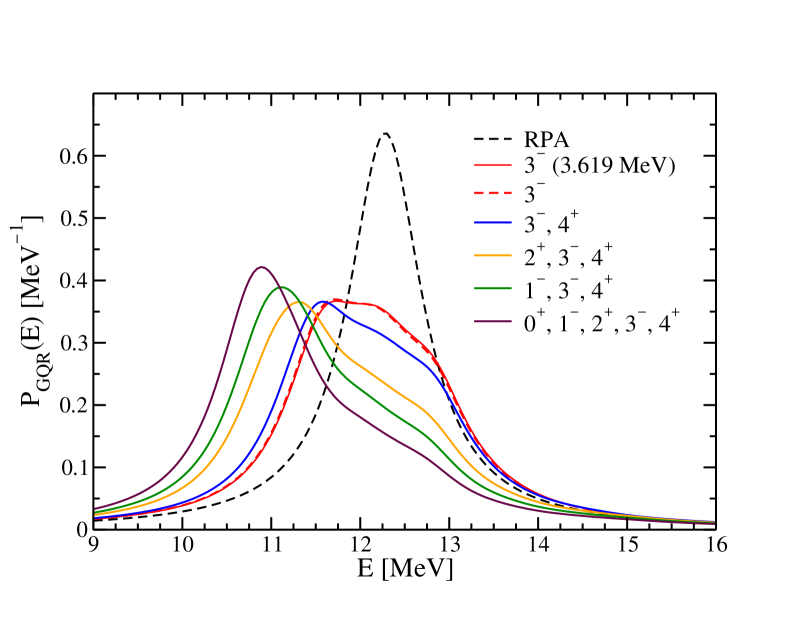
Figure 5: (color online) Probability $P$ per unit energy to find the ISGQR at an energy $E$ in ²⁰⁸Pb. Each line corresponds to the probability obtained when the phonons listed in the legend are used as intermediate states (for the selection criteria of the phonons we refer to the main text). The red-solid line is the probability we get when only the low-lying $3^{-}$ phonon at 3.61 MeV is considered as intermediate state. The label RPA (black-dashed line) refers to the RPA result, in which none of the diagrams in Fig. 4 are taken into account, but a lorentzian averaging with functions having 1 MeV width is introduced.

The result for the probability of finding the ISGQR, calculated by including in the diagrams an increasing number of intermediate phonons is displayed in Fig. 5. The RPA model space is the same used for the computation of the decay width. Phonons with multipolarity ranging from 0 to 4 and with natural parity $(-1)^{\lambda}$, have been considered. Only those having energy smaller than 30 MeV and fraction of the total isoscalar and isovector EWSR larger than 5% have been selected as intermediate states. The most important contribution to the spreading width $\Gamma^{\downarrow}$ of the resonance is given by the low-lying $3^{-}$ state, while the other phonons do contribute basically only to the energy shift. We obtain eventually a spreading width $\Gamma^{\downarrow}$ of the order of 2 MeV, and the energy centroid of the resonance is shifted down, as compared to the RPA value, to 10.9 MeV. These results are in good agreement with the experimental findings, that give a spreading width of $2.4\pm 0.4$ Bertrand et al. (1980).

Table 3: Decay width to the low-lying $3^{-}$ for the interactions used, calculated including beyond RPA contributions for the two nuclei ²⁰⁸Pb and ⁹⁰Zr. In particular, for ²⁰⁸Pb the results from Ref. Speth et al. (1985) and Ref. Bortignon et al. (1984) are also listed and in the last row, and the experimental value from Ref. Beene et al. (1989) is provided as well.

		208Pb			90Zr
Interaction		$E_{\text{trans}}$ [MeV]	$\Gamma_{\gamma}$ [eV]		$E_{\text{trans}}$ [MeV]	$\Gamma_{\gamma}$ [eV]
SLy5		$8.66$	$3.39$		$12.51$	$5.81$
SGII		$8.58$	$29.18$		$12.16$	$50.58$
SkP		$6.99$	$8.34$		$10.42$	$5.14$
LNS		$8.90$	$39.87$		$12.72$	$16.95$
Ref. Bortignon et al. (1984)		$8.59$	$3.5$			–
Ref. Speth et al. (1985)		$7.99$	$4$			–
Ref. Beene et al. (1989)		$7.99$	5$\pm$5			–

Table 4: The various quenching factors that combine to produce the decay width $\Gamma_{\gamma}$ from a typical particle-hole dipole transition, for ²⁰⁸Pb. The decay width reported here refers to a cutoff of 5% on the percentage of isovector EWSR for the dipole states. The same quantities from Bortignon et al. (1984) are displayed.

	SLy5	SGII	SkP	LNS	Ref. Bortignon et al. (1984)
Ph transition [eV]	$10^{3}$	$10^{3}$	$10^{3}$	$10^{3}$	$10^{3}$
Recoupling coefficient	3	3	3	3	3
$\pi$ – $\nu$ cancellation	5	4	3–4	4	4
p – h cancellation	3–4	2–3	2–3	3–4	2–3
Polarization	6	3	7–8	4	15
$\Gamma_{\gamma}$ [eV]	3.39	29.18	8.34	39.87	3.50

III.3 ISGQR decay to the low-lying 3^- state

In Table 3 the results obtained for the decay of the ISGQR to the low-lying octupole state in ²⁰⁸Pb and ⁹⁰Zr are shown. These correspond to a choice of the lower cutoff of 5% on the dipole EWSR of the states considered to calculate the polarization and a parameter $\eta=2$ MeV (for ²⁰⁸Pb) and $\eta=3.5$ MeV for ⁹⁰Zr; these inputs will be clarified and discussed later in the text. For completeness, the values found in literature Speth et al. (1985); Bortignon et al. (1984) for ²⁰⁸Pb are listed as well. These are all theoretical results obtained using different models: in Ref. Speth et al. (1985), the Theory of Finite Fermi Systems (cf. Ref. Speth et al. (1977)) with a phenomenological interaction is used to calculate the decay width, while in Ref. Bortignon et al. (1984) the decay width is obtained by means of the NFT, with a separable interaction at the particle-vibration vertex.

Table 5: The effect on the $\gamma$-decay width $\Gamma_{\gamma}$ of the width $\Gamma_{D}$ of the intermetiate dipole states. All the states exhausting the EWSR for more than 5% are considered. The decay width is an almost monotonically non-decreasing function of this parameter, as expected from the Bohr-Mottelson model Bohr and Mottelson (1975).

	$\Gamma_{D}$ [MeV]	$0.01$	$0.1$	$0.5$	$1.0$	$2.0$	$3.0$	$4.0$	$5.0$
$\Gamma_{\gamma}$ [eV]	SLy5	$2.34$	$2.35$	$2.46$	$2.69$	$3.39$	$4.32$	$5.34$	$6.36$
	SGII	$27.28$	$27.19$	$27.00$	$27.25$	$29.18$	$32.68$	$37.21$	$42.25$
	SkP	$7.35$	$7.35$	$7.40$	$7.59$	$8.34$	$9.54$	$11.08$	$12.86$
	LNS	$37.93$	$37.82$	$37.55$	$37.76$	$39.87$	$43.84$	$49.03$	$54.86$

We discuss here in detail the results we obtain for the decay of the ISGQR in ²⁰⁸Pb. It can be noticed that only two interactions, namely SLy5 and SkP, can reasonably reproduce the experimental value for the decay width. Nevertheless, all these forces are able to produce a total $\Gamma_{\gamma}(\text{ISGQR}\rightarrow 3^{-})$ which is only a few percent of $\Gamma_{\gamma}(\text{ISGQR}\rightarrow\text{g.s.})$, as the experiment indicates.

In order to understand which of the factors that appear in the several contributions to the decay width has a major effect on the resulting values, we have analyzed the sensitivity to the physical inputs in great detail. Table 4 displays, for the four forces used, the contribution of the several factors included in Eq. (5). Similar factors from Ref. Bortignon et al. (1984) are provided as well. The decay width that is obtained considering a typical particle-hole transition is of the order of $\approx$ keV and can be qualitatively accounted by means of the Weisskopf estimation for the reduced transition probability of a single particle excitation Bohr and Mottelson (1969). The label recoupling coefficient indicates the quenching deriving from the mismatch of angular momenta of the particles involved in the process. Then, because of the isovector nature of the operator (1), diagrams involving protons and neutrons have opposite sign and partially cancel each other. Moreover, diagrams in which the operator acts on a particle line must have an opposite sign to the ones in which it acts on a hole line, reflecting the correlations between particles and holes in vibrations Bertsch et al. (1983), resulting in a compensation of the two contributions. Eventually, the polarization contribution (6), deriving from the screening of the external field by the mediation of the giant dipole resonance, represent a further and more important quenching of the original decay width, giving then a final width of the order of electronvolts.

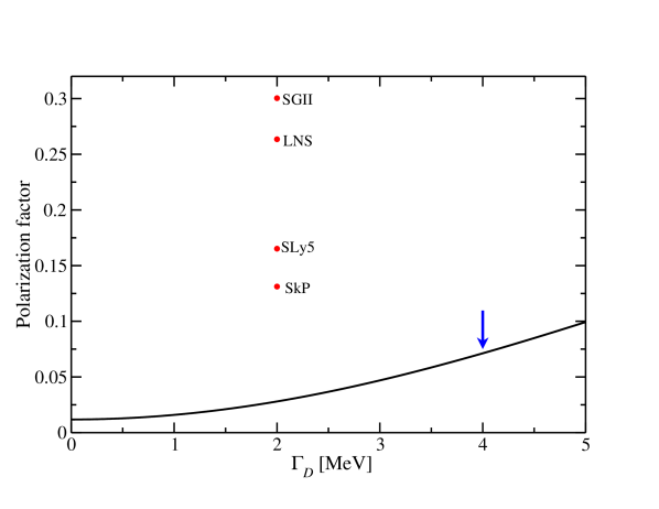
Figure 6: (color online) Polarization contribution in the separable framework as a function of the parameter $\Gamma_{D}$ (solid line). The arrow indicates the value used in Ref. Bortignon et al. (1984). The points are the analogous factors obtained within our model in which all the dipole states having a fraction of EWSR larger than 5% are considered and each one is given a width $\Gamma_{D}=2$ MeV.

We have studied in particular which assumptions and choices affect the quenching associated with the polarization contribution. First of all, in Table 5, the variation of the $\gamma$-decay width $\Gamma_{\gamma}$ with the parameter $\eta=\frac{\Gamma_{D}}{2}$ that appears in Eq. (6) as imaginary part of the energy denominator, is discussed. If only a single dipole intermediate state is considered, as in Ref. Bortignon et al. (1984), this parameter should be set equal to the IVGDR width ($\sim$4 MeV); since in our model, the dipole strength is fragmented, we should take a smaller value and we give here the trend of the decay width as a function of this parameter. As indicated by the plot in Fig. 6, the polarization factor (and consequently the decay width) should be monotonically non-decreasing when $\Gamma_{D}$ increases and reaches a roughly constant value as $\Gamma_{D}$ goes to zero. In the same plot, the points represent the polarization factors that we obtain using the value 2 MeV for the parameter $\Gamma_{D}$, but including all the dipole states having a fraction of EWSR larger than 5%. This value has been chosen in order give a width of the RPA dipole states, each convoluted with a lorentzian of width equal to $\Gamma_{D}$, similar to the experimental IVGDR width. The polarization that we get is then consistent with the one of Bohr-Mottelson model Bohr and Mottelson (1975), indicated with the arrow in Fig. 6.

We need a lower cutoff on the collectivity of the intermediate states for at least two reasons: firstly, RPA is known to be not reliable for non-collective states, and secondly, introducing them would oblige to take into account the issue of the Pauli principle correction. We then choose 5% as lower bound of the isovector and isoscalar EWSR, in keeping with several previous works, e.g., Ref. Colò et al. (2010).

A similar analysis carried out on the $\gamma$-decay of the ISGQR in ⁹⁰Zr into the lowest $3^{-}$ state would bring to analogous conclusions: the most important effect is the polarization of the nuclear medium through the excitation of dipole states. Even in this case the general result is that the decay width to the octupole state is few percent of the one to the ground-state. Results from the previously mentioned recent experiment Nicolini et al. (2011), are not yet available.

IV Conclusions

Our work is motivated by the fact that we deem it is timely to dispose of a fully-microscopic description of some exclusive properties of giant resonances, like the $\gamma$-decay. In particular, the $\gamma$-decay has been studied in the past decades using only phenomenological models. Therefore, we have implemented a scheme in which the single particle states are obtained within HF, the vibrations are calculated using fully self-consistent RPA and the whole Skyrme force is employed at the particle-vibration vertices. We treat the ground-state decay within the fully self-consistent RPA and the decay to low-lying collective vibrations at the lowest contributing order of perturbation theory beyond RPA.

We have applied our model to the $\gamma$-decay of the isoscalar giant quadrupole resonance in ²⁰⁸Pb and ⁹⁰Zr into the ground-state and the first low-lying octupole vibration. In particular, in ²⁰⁸Pb, in the case of the ground-state decay, we find that our outcomes are consistent with previous theoretical calculations, based on phenomenological models, and with the experimental data. In particular, all the Skyrme parametrizations give a $\gamma$-decay width to the ground-state of the order of hundreds of electronvolts, though, at the same time, they tend to overestimate it: these discrepancies are due to the fact that the energy of the resonance does not completely agree with the experimental data. For this reason, we conclude that the $\gamma$-decay to the ground-state is not so able to discriminate between different models, at least not more than other inclusive observable (as energy and strength).

On the other hand, the $\gamma$-decay to low-lying collective states is more sensitive to the interaction used. As a matter of fact, only two interactions (namely SLy5 and SkP) manage to achieve a decay width of few electronvolts, consistently with the experimental finding. In the case of SLy5, this fact is consistent with the good features that this parameter set has, as far as spin-independent processes are concerned (correct value of the nuclear incompressibility, reasonable fit of the neutron matter equation of state, good isovector properties). Nonetheless, the other interactions give a width $\Gamma_{\gamma}$ that is of the order of tens of electronvolts and it is very much quenched with respect to the decay width associated with a single particle transition. It is quite remarkable that our calculation, being parameter-free, reproduces numbers that are several orders of magnitude smaller than the nuclear scale of $\approx$ MeV. In particular, the description of the dipole spectrum is a crucial point, because small differences in the strength of the dipole states, introduced as intermediate states, change significantly the polarization of the nuclear medium. For ⁹⁰Zr, the general conclusion is similar: the $\gamma$-decay to low-lying collective states seems to be a good observable to test the quality of different Skyrme models, being very sensitive to the description of the polarization of the nuclear medium.

*

Appendix A Calculation of the diagrams associated with the decay between vibrational states

Figure 7: Particle-vibration coupling vertices

In this Appendix, we provide some details about the calculation of the diagrams shown in Fig. 2.

Within the PVC theory, four particle-phonon vertices are possible (cf. Fig. 7), depending whether the fermionic states involved are particles or holes. They are related by the particle-hole coniugation operator (cf. Ref. Bohr and Mottelson (1975)), so that all the vertices can be brought back to $\Lambda_{p^{\prime}p}^{J}$. From the Appendix of Ref. Colò et al. (2010), we get for the first vertex $\Lambda_{p^{\prime}p}^{J}$

$$\Lambda_{p^{\prime}p}^{J} = \langle j_{p^{\prime}}m_{p^{\prime}}|V|j_{p}m_{p},nJM\rangle$$

$$= (-)^{j_{p^{\prime}}-m_{p^{\prime}}}\begin{pmatrix}j_{p^{\prime}}&j_{p}&J\\ m_{p^{\prime}}&-m_{p}&-M\\ \end{pmatrix}\langle p^{\prime}\|V\|p,nJ\rangle.$$

For example, let us now consider the vertex $\Lambda_{hh^{\prime}}^{J}$. We can move the hole states from the initial to final state (and viceversa) by adding an appropriate phase factor.

$$\Lambda_{hh^{\prime}}^{J} = \langle(j_{h^{\prime}}m_{h^{\prime}})^{-1}|V|(j_{h}m_{h})^{-1},nJM\rangle$$

$$= (-)^{j_{h^{\prime}}+m_{h^{\prime}}+j_{h}-m_{h}}\langle j_{h}-m_{h}|V|j_{h^{\prime}}-m_{h^{\prime}},nJM\rangle$$

$$= (-)^{j_{h^{\prime}}-m_{h^{\prime}}}\begin{pmatrix}j_{h}&j_{h^{\prime}}&J\\ -m_{h}&m_{h^{\prime}}&-M\\ \end{pmatrix}\langle h\|V\|h^{\prime},nJ\rangle$$

which is equal to $\Lambda_{p^{\prime}p}^{J}$ after the identification $h^{\prime}\leftrightarrow p$ and $h\leftrightarrow p^{\prime}$, except for the phase factor. Similar relations can be established between $\Lambda_{p^{\prime}p}^{J}$ and $\Lambda_{ph}^{J}$ or $\Lambda_{hp}^{J}$. Moreover, the vertices in which the phonon is created instead of annihilated can be derived from these latter by adding a phase factor $(-)^{J+M}$, changing the sign of the projection $M$ of the angular momentum $J$ of the phonon and using the following expression for the reduced matrix element of the interaction

$$\langle i,nJ\|V\|j\rangle = \sqrt{2J+1}(-)^{J+j_{j}-j_{i}}\sum_{ph}X_{ph}^{nJ}V_{J}(jhip)$$

$$+(-)^{j_{h}-j_{p}+J}Y_{ph}^{nJ}V_{J}(jpih).$$

These PVC vertices are then used to evaluate the diagrams in Fig. 2. In the following, one of them (namely Fig. 22) is calculated in detail. For each particle-phonon vertex, we have a reduced matrix element of the interaction multiplied by a 3-j symbol that takes care of the coupling of angular momenta. Moreover, the single-particle operator $Q_{\lambda}$ brings another 3-j symbol and a matrix element. Eventually, the last 3-j symbol, matching the angular momentum of the initial state, of the final one and of the operator comes from the Wigner-Eckart theorem, since we need a reduced matrix element. The energy denominators are obtained by using the rules of second-order perturbation theory.

$$\left\langle n^{\prime}J^{\prime}\left\|Q_{\lambda}\right\|nJ\right\rangle_{\ref{fig:graphs}\ref{fig:graph5}} = \sum_{\begin{subarray}{c}M\mu m_{h}\\ m_{p}m_{p^{\prime}}\end{subarray}}(-)^{J-\lambda+M^{\prime}}(2J^{\prime}+1)\begin{pmatrix}J&\lambda&J^{\prime}\\ M&\mu&-M^{\prime}\\ \end{pmatrix}$$ (13)

$$\phantom{\sum_{M\mu m_{h}}}(-)^{J+M}\begin{pmatrix}j_{h}&j_{p}&J\\ m_{h}&m_{p}&-M\\ \end{pmatrix}\langle p\|V\|h,nJ\rangle$$

$$\phantom{\sum_{M\mu m_{h}}}(-)^{J^{\prime}+j_{p^{\prime}}-m_{p}}\begin{pmatrix}j_{p^{\prime}}&j_{p}&J^{\prime}\\ m_{p^{\prime}}&-m_{p}&M^{\prime}\\ \end{pmatrix}\langle p^{\prime},n^{\prime}J^{\prime}\|V\|p\rangle$$

$$\phantom{\sum_{M\mu m_{h}}}\begin{pmatrix}j_{h}&j_{p^{\prime}}&\lambda\\ m_{h}&m_{p^{\prime}}&\mu\\ \end{pmatrix}\frac{(-)^{j_{p^{\prime}}-j_{h}+\lambda}Q_{hp^{\prime}}^{\lambda pol}}{(E_{J}-\epsilon_{ph}+i\eta)(E_{J}-\hbar\omega_{J^{\prime}}-\epsilon_{p^{\prime}h}+i\eta^{\prime})}$$

The four 3-j symbol can be summed in one 6-j symbol by usual relations (see e.g. Ref. Brink and Satchler (1994))

$$\sum_{\begin{subarray}{c}M\mu M^{\prime}\\ m_{p}m_{p^{\prime}}\end{subarray}}(-)^{j_{p}+m_{p}+j_{p^{\prime}}+m_{p^{\prime}}+j_{h}-m_{h}} \begin{pmatrix}j_{p^{\prime}}&j_{p}&J^{\prime}\\ -m_{p^{\prime}}&m_{p}&-M^{\prime}\end{pmatrix}\begin{pmatrix}j_{p}&j_{h}&J\\ -m_{p}&-m_{h}&M\end{pmatrix}\begin{pmatrix}j_{h}&j_{p^{\prime}}&\lambda\\ m_{h}&m_{p^{\prime}}&\mu\end{pmatrix}\begin{pmatrix}J&\lambda&J\\ M&\mu&-M^{\prime}\end{pmatrix}$$ (14)

$$=-\frac{1}{\sqrt{2J^{\prime}+1}}\begin{Bmatrix}J&\lambda&J\\ j_{p^{\prime}}&j_{p}&j_{h}\end{Bmatrix}$$

We then finally get Eq. (.e)

References

• BortignonĀ etĀ al. (1998) P.Ā F.Ā Bortignon, A.Ā Bracco, Ā andĀ R.Ā A.Ā Broglia,Ā Giant Resonances. Nuclear Structure At Finite TemperatureĀ (Harwood Academic,Ā 1998).
• HarakehĀ andĀ vanĀ der Woude (2001) M.Ā N.Ā HarakehĀ andĀ A.Ā vanĀ der Woude,Ā Giant Resonances: Fundamental High-Frequency Modes of Nuclear Excitation,Ā Oxford Studies in Nuclear PhysicsĀ (Oxford University Press Inc.,Ā 2001).
• BeeneĀ etĀ al. (1989) J.Ā R.Ā Beene, F.Ā E.Ā Bertrand, M.Ā L.Ā Halbert, R.Ā L.Ā Auble, D.Ā C.Ā Hensley, D.Ā J.Ā Horen, R.Ā L.Ā Robinson, R.Ā O.Ā Sayer, Ā andĀ T.Ā P.Ā Sjoreen,Ā Phys. Rev. CĀ 39,Ā 1307 (1989).
• BeeneĀ etĀ al. (1990) J.Ā R.Ā Beene etĀ al.,Ā Phys. Rev. CĀ 41,Ā 920 (1990).
• BeeneĀ etĀ al. (1985) J.Ā R.Ā Beene, G.Ā F.Ā Bertsch, P.Ā F.Ā Bortignon, Ā andĀ R.Ā A.Ā Broglia,Ā Phys. Lett. BĀ 164,Ā 19 (1985).
• BortignonĀ etĀ al. (1984) P.Ā F.Ā Bortignon, R.Ā A.Ā Broglia, Ā andĀ G.Ā F.Ā Bertsch,Ā Phys. Lett. BĀ 148,Ā 20 (1984).
• SpethĀ etĀ al. (1985) J.Ā Speth, D.Ā Cha, V.Ā Klemt, Ā andĀ J.Ā Wambach,Ā Phys. Rev. CĀ 31,Ā 2310 (1985).
• Colò etĀ al. (1992) G.Ā Colò, P.Ā F.Ā Bortignon, N.Ā VanĀ Giai, A.Ā Bracco, Ā andĀ R.Ā A.Ā Broglia,Ā Phys. Lett. BĀ 276,Ā 279 (1992).
• Colò etĀ al. (1994) G.Ā Colò, N.Ā VanĀ Giai, P.Ā F.Ā Bortignon, Ā andĀ R.Ā A.Ā Broglia,Ā Phys. Rev. CĀ 50,Ā 1496 (1994).
• NicoliniĀ etĀ al. (2011) R.Ā Nicolini etĀ al.,Ā Acta Phys. Pol.Ā B42,Ā 653 (2011).
• deĀ ShalitĀ andĀ Feshbach (1990) A.Ā deĀ ShalitĀ andĀ H.Ā Feshbach,Ā Nuclear StructureĀ (John Wiley and Sons Inc.,Ā 1990).
• Rowe (1970) D.Ā J.Ā Rowe,Ā Nuclear Collective MotionĀ (Methuen,Ā 1970).
• BesĀ etĀ al. (1974) D.Ā R.Ā Bes, G.Ā G.Ā Dussel, R.Ā A.Ā Broglia, R.Ā J.Ā Liotta, Ā andĀ B.Ā R.Ā Mottelson,Ā Phys. Lett. BĀ 52,Ā 253 (1974).
• BortignonĀ etĀ al. (1977) P.Ā F.Ā Bortignon, R.Ā A.Ā Broglia, D.Ā R.Ā Bes, Ā andĀ R.Ā Liotta,Ā Phys. Rep.Ā 30,Ā 305 (1977).
• Colò etĀ al. (2007) G.Ā Colò, P.Ā F.Ā Bortignon, S.Ā Fracasso, Ā andĀ N.Ā VanĀ Giai,Ā Nucl. Phys.Ā A788,Ā 173 (2007),Ā Proceedings of the 2nd International Conference on Collective Motion in Nuclei under Extreme ConditionsĀ -Ā COMEX 2.
• Colò etĀ al. (2010) G.Ā Colò, H.Ā Sagawa, Ā andĀ P.Ā F.Ā Bortignon,Ā Phys. Rev. CĀ 82,Ā 064307 (2010).
• ChabanatĀ etĀ al. (1998) E.Ā Chabanat, P.Ā Bonche, P.Ā Haensel, J.Ā Meyer, Ā andĀ R.Ā Schaeffer,Ā Nucl. Phys.Ā A635,Ā 231 (1998).
• VanĀ GiaiĀ andĀ Sagawa (1981) N.Ā VanĀ GiaiĀ andĀ H.Ā Sagawa,Ā Phys. Lett. BĀ 106,Ā 379 (1981).
• DobaczewskiĀ etĀ al. (1984) J.Ā Dobaczewski, H.Ā Flocard, Ā andĀ J.Ā Treiner,Ā Nucl. Phys.Ā A422,Ā 103 (1984).
• CaoĀ etĀ al. (2006) L.Ā G.Ā Cao, U.Ā Lombardo, C.Ā W.Ā Shen, Ā andĀ N.Ā V.Ā Giai,Ā Phys. Rev. CĀ 73,Ā 014313 (2006).
• Martin (2007) M.Ā J.Ā Martin,Ā Nucl. Data SheetsĀ 108,Ā 1583 (2007).
• BortignonĀ andĀ Broglia (1981) P.Ā F.Ā BortignonĀ andĀ R.Ā A.Ā Broglia,Ā Nucl. Phys.Ā A371,Ā 405 (1981).
• SpethĀ etĀ al. (1977) J.Ā Speth, E.Ā Werner, Ā andĀ W.Ā Wild,Ā Phys. Rep.Ā 33,Ā 127 (1977).
• BertschĀ etĀ al. (1983) G.Ā F.Ā Bertsch, P.Ā F.Ā Bortignon, Ā andĀ R.Ā A.Ā Broglia,Ā Rev. Mod. Phys.Ā 55,Ā 287 (1983).
• BertrandĀ etĀ al. (1980) F.Ā E.Ā Bertrand, G.Ā R.Ā Satchler, D.Ā J.Ā Horen, J.Ā R.Ā Wu, A.Ā D.Ā Bacher, G.Ā T.Ā Emery, W.Ā P.Ā Jones, D.Ā W.Ā Miller, Ā andĀ A.Ā vanĀ der Woude,Ā Phys. Rev. CĀ 22,Ā 1832 (1980).
• BohrĀ andĀ Mottelson (1975) A.Ā BohrĀ andĀ B.Ā R.Ā Mottelson,Ā Nuclear Stucture,Ā Vol.Ā IIĀ (W. A.Benjamin Inc.,Ā 1975).
• BohrĀ andĀ Mottelson (1969) A.Ā BohrĀ andĀ B.Ā R.Ā Mottelson,Ā Nuclear Stucture,Ā Vol.Ā IĀ (W. A.Benjamin Inc.,Ā 1969).
• BrinkĀ andĀ Satchler (1994) D.Ā M.Ā BrinkĀ andĀ G.Ā R.Ā Satchler,Ā Angular Momentum,Ā 3rdĀ ed.Ā (Oxford University Press Inc.,Ā 1994).