Bucket Shaking Stops Bunch Oscillations In The Tevatron

Abstract

Bunches in the Tevatron are known to exhibit longitudinal oscillations which persist indefinitely. These oscillations are colloquially called “dancing bunches”. Although the dancing bunches do not cause single bunch emittance growth or beam loss at injection, it leads to bunch lengthening at collisions. In operations, a longitudinal damper has been built which stops this dance and damps out coupled bunch modes. Recent theoretical work predicts that the dance can also be stopped by an appropriate change in the bunch distribution. This paper shows the Tevatron experiments which support this theory.

I Introduction

Ever since the start of Run II, the bunches in the Tevatron have been observed to have longitudinal oscillations which persist indefinitely. The reason for the persistence of these oscillations have been traced to the loss of Landau damping (LLD) caused by the inductive impedance of the Tevatron ronmoore ; these oscillations are colloquially called ”dancing bunches”. At the injection energy of 150 GeV, these oscillations do not seem to yield any emittance growth or any beam loss. But at the flattop energy of 980 GeV, they lead to an effective bunch length growth which reduces luminosity. In order to stop the dance, a longitudinal damper system has been built which damps it out dampers .

Recently, theoretical work has predicted that the dance can also be stopped by flattening out its phase space distribution at low synchrotron frequencies burov1 ; burov2 . In particular, this flattening can be achieved by shaking the RF phase at the synchrotron frequency of the low amplitude particles burov3 . The goal of this paper is to demonstrate experimentally that the dance can be stopped by changing the beam distribution appropriately.

II Theory

The Boltzmann-Jeans-Vlasov (BJV) equation henon is conventionally used to describe longitudinal motion of bunched beams. This equation has a continuous spectrum and, possibly, a discrete one kampen ; ecker . The discrete van Kampen modes are described with regular functions and some of them do not decay. Therefore, in principle, any coupled bunch wake drives an instability when there is LLD. However, in practice, the coupled bunch wake has to be high enough to give an observable growth rate. If the growth rate is too small, LLD results in persistent oscillations caused by initial perturbations.

For bunched beams, LLD was first discussed and estimated by F. Sacherer sacherer . Later, his main results were re-derived and discussed in more details by other authors besnier ; hofmann ; ng ; metral ; gonzalez . For a dipole mode, all the approaches were actually based on an assumption that the bunch moves as a rigid body. However, recent solutions of the eigenvalue problem burov1 ; burov2 show that the rigid bunch approximation can lead to significant over estimations of the LLD threshold.

As it is known since the original Sacherer’s paper sacherer , the threshold bunch population $N_{\rm th}$ is a strong function of the bunch length $\ell$. In particular, for an inductive wake above transition,

$$N_{\rm th}\propto\ell^{5}.$$ (1)

This scaling law can be derived from an idea that Landau damping is lost whenever the incoherent tune shift $\Delta\Omega\propto NZ_{||}(\ell^{-1})/\ell^{2}$ exceeds the incoherent tune spread $\delta\Omega\propto\ell^{2}$. For the inductive impedance, the incoherent tune shift decreases with the bunch length as $\Delta\Omega\propto\ell^{-3}$. The combined action of this decrease with increasing nonlinear tune spread $\delta\Omega\propto\ell^{2}$ results in $\ell^{5}$ in Eq. 1. This high sensitivity on the bunch length indicates that approximations of the bunch profile or arbitrary assumptions about the eigenfunctions can lead to significant errors in the calculated LLD threshold because they can change the effective bunch length. For example, for a full bucket of a single-harmonic RF system with an inductive impedance above transition, the threshold relative tune shift $\Delta\Omega/\Omega$ was found to be as low as 10% for the Hofmann-Pedersen distribution, and just $\sim\!1$% for a model of the Tevatron coalesced bunch burov1 . In terms of bunch population, the two thresholds differ by almost two orders of magnitude. It turns out that the onset of LLD is highly sensitive to the steepness of the distribution function at low amplitudes: the flatter the distribution, the more stable it is. This prediction appears to be generally correct when the bare RF synchrotron frequency monotonically decreases with amplitude and the wake field is repulsive, i.e. the wake lowers the incoherent synchrotron frequencies. This conclusion agrees with Ref. metral , where the LLD threshold was calculated for several distributions with the inductive impedance above and below transition. It was shown there that below transition LLD is sensitive to the edges of the distribution, while above transition, it is sensitive to the flatness of the bunch core.

As was discussed in Ref. burov1 , in the case of a sinusoidal RF system, any combination of inductance, wall resistivity, or high order cavity modes above transition, or space charge below transition will shift the incoherent spectrum down to lower frequency and the coherent mode emerges above it. Since the incoherent frequencies of low amplitude particles are close to the mode frequency, their wieght in the mode dominates. Hence, for a single-harmonic RF and a repulsive wake function, the discrete mode causes dipole motion of the bunch center while its tails remain still. This is the behavior of the bunches in the Tevatron ronmoore .

II.1 Flattening out the distribution for particles with small amplitudes

To flatten out the bunch distribution at small amplitudes, resonant shaking of the RF phase was suggested for the Tevatron burov3 , with an idea to use anomalous diffusion within a controlled phase space area; see Ref.jeon ; huang ; syleebook and references therein.

Let it be assumed that the RF phase is modulated at a frequency $\Omega_{m}$, which is close to the synchrotron frequency $\Omega_{s}$. Let the amplitude of the modulation $\phi_{m}(t)$ adiabatically grow from zero, then stay a while at some value $\phi_{0}$ and then adiabatically decrease to zero. To prevent excitation of the tail particles and the coherent modes, the process has to be adiabatic. However, even when the process is generally adiabatic, i.e. when $|d\phi_{m}/dt|\ll\Omega_{s}\phi_{0}$, the adiabaticity for some particles is going to be broken. Indeed, resonant RF shaking results in either one or two stable fixed points (SFPs) inside the bucket. In the last case, there is an inner separatrix between the two SFPs and when the modulation amplitude changes, the separatrix moves and some particles cross it. Separatrix crossing is a non-adiabatic process resulting in classical chaos and anomalous diffusion.

Thus, the phase space density can be changed only in the case of two SFPs which occur when the modulation frequency is lower than the synchrotron frequency, $\Omega_{m}<\Omega_{s}$, and the modulation amplitude is lower than its bifurcation value, $\phi_{m}<\phi_{b}=3.08\epsilon^{3/2}$ with $\epsilon=1-\Omega_{m}/\Omega_{s}$. When the modulation amplitude grows from zero to its bifurcation value, and when it comes back to zero later, the irreversible change of the phase space density occurs for the phase space area with action $J\leq J_{\lim}$, where

$$J_{\lim}\approx 6\epsilon J_{\rm{bucket}},$$ (2)

and $J_{\rm{bucket}}$ is the bucket acceptance. For dimensionless variables associated with the unperturbed Hamiltonian $H(z,p)=p^{2}/2+1-\cos z$, the acceptance $J_{\rm{bucket}}=8/\pi$. The numerical factor “6” in Eq. (2) was approximated from a numerical solution discussed below and it is about two times larger than the separatrix border at zero amplitude. After this adiabatic cycle, the phase space density becomes nearly constant for the entire area $J<J_{\lim}$, provided that the shaking amplitude crosses its bifurcation value, i.e.

$$\phi_{0}\geq 3.08\epsilon^{3/2}$$ (3)

It is worth mentioning that the adiabatically ramped modulation does not excite any coherent motion when the modulation is turned off. Thus, to make a flat phase space density within a certain action $J_{\lim}$, the adiabatic RF phase modulation has to be applied slightly below the synchrotron frequency, $\epsilon=0.16J_{\lim}/J_{\rm{bucket}}$, and its amplitude must cross the bifurcation, Eq. (3).

A simulation of how the bunch distribution is modified with RF phase shaking has been done using the following map

$$z_{n+1} =z_{n}+p_{n}\Delta t$$

$$p_{n+1} =p_{n}-\Delta t\sin\bigg{[}z_{n+1}-\phi_{m}(t_{n})\sin(1-\epsilon)t_{n}\bigg{]}$$ (4)

$$t_{n+1} =t_{n}+\Delta t$$

where $z_{n}$ and $p_{n}$ are the coordinate and momenta respectively in dimensionless units, $t_{n}$ is the time variable in radians of the synchrotron oscillation, $\Delta t$ is its numerical step. The amplitude of the RF phase modulation $\phi_{m}(t)$ was taken as a trapezoid similar to Fig. 4.

Here are the typical parameters used in the simulations:

• the adiabaticity parameter $\dot{\phi_{m}}/(\Omega_{s}\phi_{0})\sim 200$.

• $\Delta t=0.01$ radians which is small enough for the results to be independent of its specific value.

• Initial phase space density is assumed to be $F(J)\propto(J_{\rm max}-J)^{2}$ with the emittance $J_{\rm max}$ set close to the bucket acceptance.

• Number of macro-particles $N=4\times 10^{4}$.

The simulation results before and after shaking are shown in Fig. 1 for $\epsilon=0.03$, $\phi_{0}=0.025$ and two consecutive shaking cycles with $T_{\rm{sim}}=600$ radians or about 90 synchrotron periods each. Each cycle time was equally divided into three parts of about 30 synchrotron periods each: a linear growth of the modulation amplitude from 0 to $\phi_{0}$, staying at $\phi_{0}$, and a linear decrease from $\phi_{0}$ back to 0.

Clearly the action distribution PDF[J] has successfully flattened out and there is even a little divot that is less pronounced after the second shaking cycle. Except for this small difference, the second cycle does not significantly change the distribution. The phase distribution PDF[$\psi$] after every cycle is as flat as before, showing that no coherent oscillations were excited.

The time dependence of the unperturbed Hamiltonian $H(z,p)=p^{2}/2+(1-\cos z)$ calculated for the bunch average values of the canonical variables $\langle z\rangle$ and $\langle p\rangle$ is shown in Fig. 2. This simulation shows that the adiabaticity of shaking is really important: after every cycle, the Hamiltonian goes to zero. The irregular features of this plot probably reflect the chaotic nature of the anomalous diffusion responsible for the flattening of the distribution.

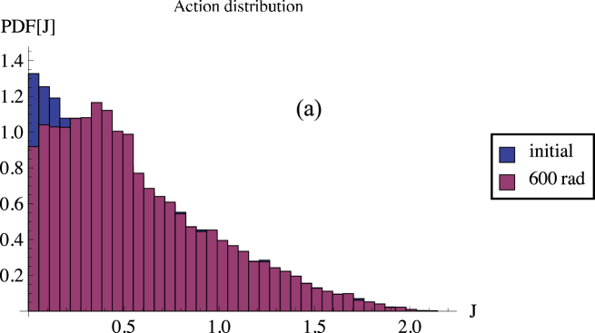
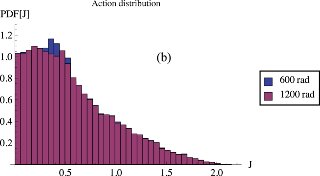
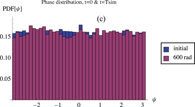
Figure 1: (a) distributions over action PDF[J], original (blue) and after the first ramp (pink); the overlapped area is in violet. (b) a similar comparison of the distributions before and after the second ramp. (c) a comparison of the phase distributions PDF[$\psi$] before and after the first ramp.

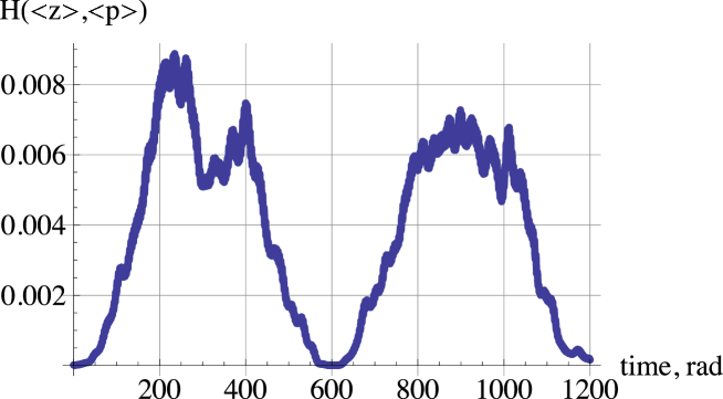
Figure 2: Time dependence of the unperturbed Hamiltonian taken for the bunch-average coordinate and momentum.

III Experiment

The block diagram of the phase modulation hardware used for shaking the beam is shown in Fig. 3. A signal generator generates a sine wave where its amplitude and frequency can be programmed and its output is fed into a phase shifter module. The phase shifter modulates the Tevatron low level RF (LLRF) and the result is fed into the Tevatron high level RF (HLRF). Essentially, the block diagram produces the following

$$f_{\rm HLRF}=A\sin\bigg{[}2\pi f_{\rm LLRF}t+\phi_{m}(t)\sin(2\pi f_{m}t)+\theta\bigg{]}$$ (5)

where $f_{\rm HLRF}$ is the phase modulated signal sent to the HLRF, $A$ is the amplitude of the signal sent to the HLRF, $f_{\rm LLRF}$ is the frequency from the LLRF, $\theta$ is an arbitrary phase, and the signal generator produces the amplitude $\phi_{m}$ and frequency $f_{m}$ for the phase modulation.

Figure 3: The block diagrams of the bunch shaker and detectors used to monitor the bunches for the experiments.

The time evolution of the bunch during the experiment are measured using the Sampled Bunch Display (SBD) pordes . Its block diagram is shown in Fig. 3. The SBD measures the bunch profile from a resistive wall current monitor with an oscilloscope that has a 2 GHz bandwidth and the collected data is processed with a LabView program which calculates the following parameters:

• bunch centroid,

• bunch current,

• rms bunch length.

These parameters are then returned to the control system and can be plotted to give Figures 5 and 9. Furthermore, the snapshots of the bunch from the resistive wall signal can also be downloaded. The SBD trigger has been set up to take five consecutive snapshots of the bunch that are 1 s apart. These snapshots are presented in the figures below.

The block diagram of the phase detector used to measure the longitudinal motion of the bunch w.r.t. the Tevatron RF is shown in Fig. 3. The $I/Q$ phase detector is a part of the Tevatron longitudinal damper system dampers which essentially takes the sum signal from a stripline pickup, down-converts it with the Tevatron LLRF and low pass filters it to produce a quadrature signal. The quadrature signal is then measured with a spectrum analyzer.

The Tevatron parameters relevant to the experiment are shown in Table 1. This experiment only uses two coalesced proton bunches and measurements are either taken at the injection energy of 150 GeV or at the flattop energy of 980 GeV.

Table 1: Tevatron Parameters Relevant To The Experiment

Parameter	Value	Units
Injection energy	150	GeV
Flattop energy	980	GeV
Synchrotron frequency at 150 GeV	$87.47$	Hz
Synchrotron frequency at 980 GeV	$34.75$	Hz
RF frequency at 150 GeV	$53.103$	MHz
RF frequency at 980 GeV	$53.104$	MHz
Harmonic number	1113	–
Buckets between two injected bunches	21	–
Intensity per bunch	$(200-300)\times 10^{9}$	–

III.1 Results at the injection energy of 150 GeV

The results in this section have been performed at the injection energy of 150 GeV. At injection, the bunch nearly fills the bucket and so there are small beam current losses whenever the bunch is shaken. (Results at flattop do not have this problem. See section III.2). In this experiment, $f_{m}$ has been set to $87.47$ Hz because it is the measured synchrotron frequency $f_{s}$ and the bunch is shaken one time for 14 s. (Note: theoretically, $f_{m}$ should have been set to a frequency which is smaller than $f_{s}$. However, at the time, this criterion was not appreciated and the experiment was not done.) The phase ramp used in the 150 GeV experiments is not adiabatic and is shown in Fig. 4. The maximum amplitude of the shake has been tested for $\phi_{0}=1^{\circ}$, $2^{\circ}$ and $3^{\circ}$ respectively and experimentally, $\phi_{0}=3^{\circ}$ has been found to produce the best effect for the duration of the shake.

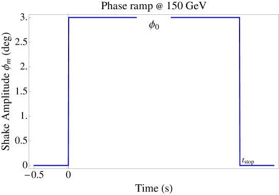
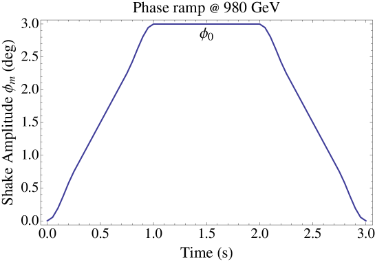
Figure 4: These are the phase ramps $\phi_{m}(t)$ used at 150 GeV and 980 GeV. For the 150 GeV experiments, $t_{\rm stop}$ is user defined.

Figure 5 shows the shake duration and the behavior of the bunch current, centroid, and rms bunch length before and after shaking. The beam current drops by about $2.3$% and the rms bunch length grows by about $1.8$% after being shaken. The beam current drop is not surprising because of the filled bucket. And the change in rms bunch length comes from the shape change which is clearly seen in Fig. 6. After the shake is turned off, a nice divot structure forms which confirms the prediction previously discussed in section II.1.

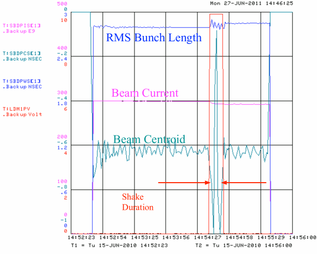
Figure 5: The data from the SBD system is plotted here: T:SBDPWS, T:SBDPIS and T:SBDPCS. The beam is shaken for 14 s and there is some beam loss and bunch length growth. Although the measured bunch centroid looks like it is still oscillating, the snapshots show that the dancing has stopped. See Fig. 6.

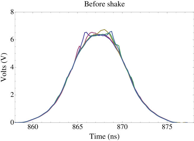
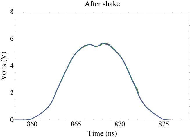
Figure 6: These are snapshots taken by the SBD before and after shaking. Before any shakes, the bunch is dancing. The result after shaking the beam for 14 s is the creation of a divot structure in the bunch and stoppage of the tip motion.

III.1.1 Contrast to Dampers

The bunch distribution after it has been shaken can be contrasted to the distribution when dampers are used instead to stop the dancing. The before and after distributions are shown in Fig. 7. The effect of dampers on the bunch distribution is to make it more triangular. This can be contrasted to the shaking technique shown in Fig. 6 where the distribution becomes more rotund. Also, after the dance stops and the dampers are turned off, the bunches do not start dancing again even after the dampers have been off for 5 min.

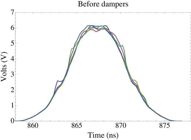
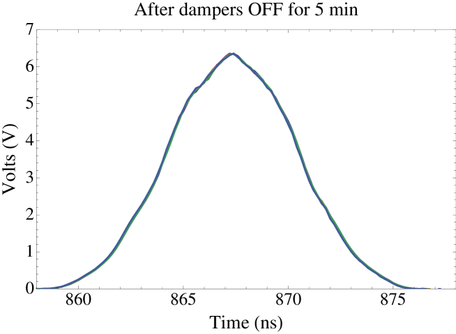
Figure 7: The before and after effects of using the damper to stop the dance. The distribution after the dampers have stopped the dancing is to make the distribution more triangular in shape.

At first glance, the stability of the bunch after the dampers are off contradicts the described theory of LLD. Indeed, according to this theory, the LLD threshold is lowered when the distribution function becomes more steep and thus the beam distribution shown in Fig. 7 has to be less stable after the dampers are turned off than it was before they were on. A resolution for this seemingly contradictory observation relies on the necessity to distinguish between LLD and instability. Indeed, if Landau damping is lost, the growth rate is determined by the coupled bunch wake forces. If these forces are weak enough, the instability takes too long to grow and so it cannot be observed. There are two types of long range wake fields that can be considered as possible candidates for driving the longitudinal coupled bunch instability (LCBI): cavity modes and the resistive wall wake. Direct calculations show that the resistive wall wake is extremely weak and has to be removed from this list. Even for 36 Tevatron bunches, the calculated resistive wall LCBI growth time is $\sim\!10$ days and so the only remaining candidate is the RF cavity modes. According to Ref. tan2005 , the LCBI observations at the top energy for 36 proton bunches can be explained by higher order modes at 311 MHz with caveats: the calculated growth time using the rigid bunch approximation is an order of magnitude faster than the measured one. There can be two reasons for this discrepancy: the first is a decreased Q-value compared to its measured value done in 2000 tan2005 ; HOM and the second is that the rigid bunch approximation overestimates both the threshold and the growth rate of the instability by several times.

III.1.2 Initial Bunch Shape Effects

The number of shaking cycles required to stop the bunch varied from case to case. Most likely, this is due to the non-optimized detuning of the shake frequency and some variations in the bunch intensities and profiles which cause variations in the incoherent tune shifts. Perhaps, a better choice of the detuning parameter $\epsilon=1-f_{m}/f_{s}$ can lead to single shake damping of the dance, but there was no opportunity to test this.

In this experiment five bunch coalescing is used rather than the usual seven. The initial bunch distribution between bunch 1 and 2 are quite different because the Main Injector has not been tuned up for five bunch coalescing. Therefore, the random effects of untuned coalescing has made bunch 1 dance a lot more than bunch 2 before shaking is applied. Figure 8 shows the result of shaking the two bunches at the same time. The bunches are shaken for $7-8$ s at $\phi_{0}=3^{\circ}$ and the first bunch does not stop dancing while the second bunch stops dancing and gets a divot.

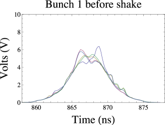
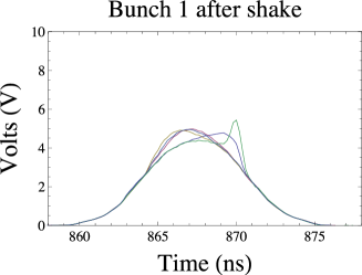
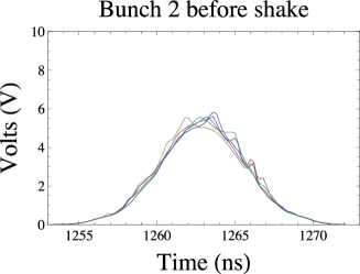
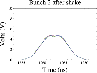
Figure 8: The initial bunch shape can have an effect on how strongly it must be shaken to stop the dancing.

III.2 Results at the flattop energy of 980 GeV

The bucket is about a factor of two larger than the beam size at 980 GeV, and thus allows the beam to freely change shape without being constrained by the bucket edges. A $\phi_{m}$ ramp has been created so that there are no abrupt changes in the RF as shown in Fig. 4. Previous experiments have shown that sudden turn-ons can cause some beam loss even though the bucket is large compared to the beam size.

In this experiment, the total time the phase is ramped is 3 s. The rise and fall time of the ramp has been chosen to be 1 s because it is slow compared to the synchrotron period of 29 ms. The flattop period can be varied, but for this experiment it has been set to 1 s.

The modulation frequency $f_{m}$ has been set to the measured synchtron tune $34.75$ Hz and the bunch is shaken seven times with the $\phi_{m}$ ramp.

Figure 9 shows the seven $\phi_{m}$ ramps and the behavior of the bunch current, centroid, and rms bunch length for the duration of the experiment. The beam current is constant throughout the experiment but the rms bunch length grows by about $18$% (from $1.67$ ns to $1.97$ ns) at the end of the experiment. It is interesting to notice that the rms bunch length grows after each shake because of the shape change. A comparison of the bunch shapes before and after the shakes shows that the rms bunch length growth comes from the flatter core of the bunch while its tails remain unchanged.

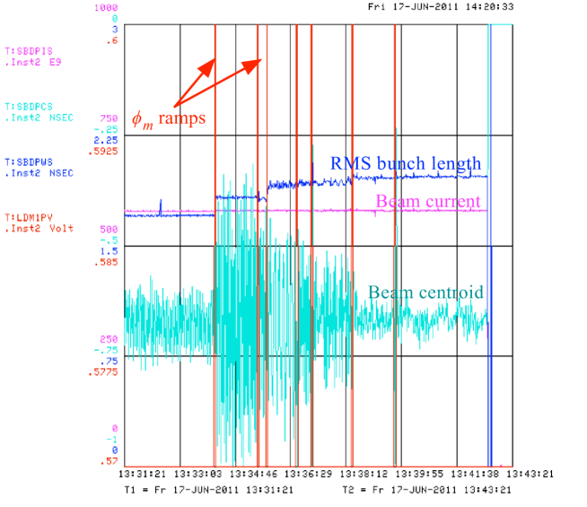
Figure 9: The beam is shaken seven times using the $\phi_{m}$ ramp shown in Fig. 4 at 980 GeV. After the seventh shake the dancing stops but there is growth in rms bunch length because of the shape change.

Figure 10 shows the bunch shape and the spectrum before shaking starts. The spectrum shows the revolution frequency and the synchrotron sidebands which are about $6$ dB smaller than the revolution harmonic. The beam has no quadrupole motion because there are no resonances at twice the synchrotron frequency.

Figure 11 shows both the the bunch shape evolution and the spectrum from the phase detector after the first, third, fifth and seventh shakes. It is clear from these plots that after the first shake the amplitude of the dance has increased by about 14 dB relative to the amplitude before shaking. And after each subsequent shake, the amplitude becomes smaller, which after the seventh shake, the dance amplitude has decreased by $14$ dB relative to the amplitude before shake. The shape of the bunch after the seventh shake has clearly changed. Figure 12 superimposes the before and after the seventh shake snapshots where the shape change is clearly evident.

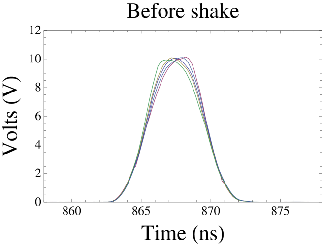
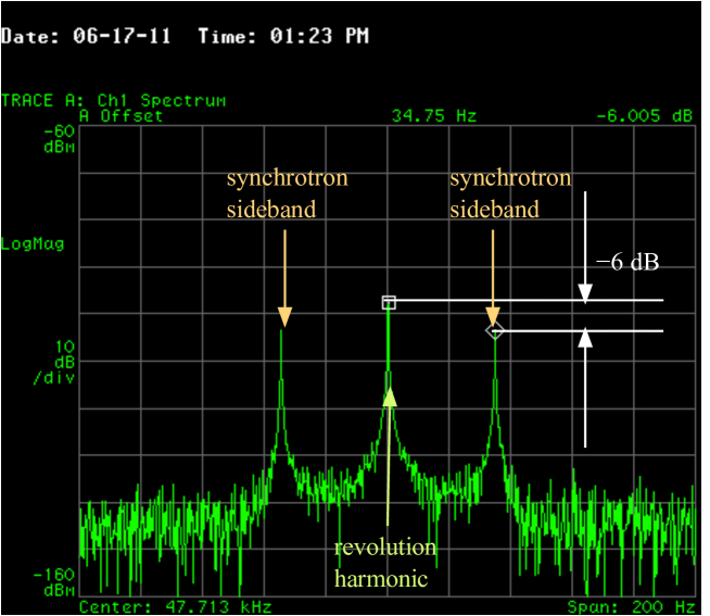
Figure 10: These figures show the bunch dancing in both the time domain and the frequency domain before any shaking is done at 980 GeV. The synchrotron sidebands which are $\pm 34.75$ Hz away from the first revolution harmonic are indicated here.

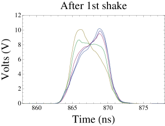
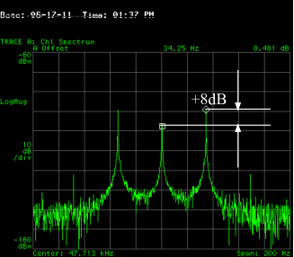
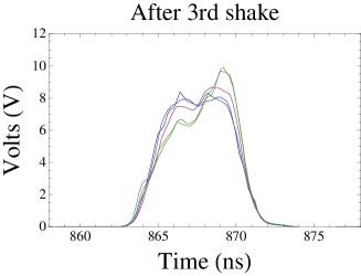
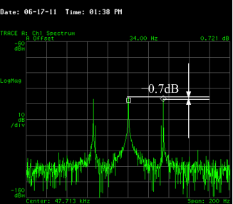
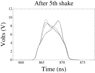
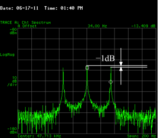
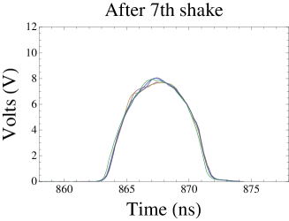
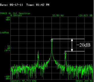
Figure 11: These figures show how the bunch shape evolves after the first, third, fifth and seventh shake. After the seventh shake, the synchrotron amplitude is reduced by about 14 dB w.r.t. its size before any shake.

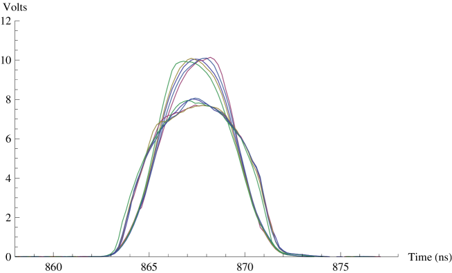
Figure 12: All the traces which are collected before and after the seventh shake are plotted together here which clearly shows the shape change at the end of the experiment.

IV Conclusion

Similar ideas for bunch distribution flattening have been suggested and implemented in the KEK-PS toyama1 ; toyama2 and the KEK Photon Factory sakanaka . This technique is also routinely applied in the CERN SPS to blow up the longitudinal emittance for stabilizing the beam shaposhnikova . However, in all these cases, narrow band RF noise around the synchrotron sidebands are excited. In the KEK-PS and SPS, the RF perturbation is applied to the voltage amplitude while at the KEK Photon Factory, noise is applied to the RF phase. The experiments described in this paper take a different approach: instead of noise, the RF phase is excited at the synchrotron frequency, and its amplitude is ramped adiabatically. This technique works because anomalous diffusion flattens the bunch distribution. It is also possible that this technique is able to finely regulate the width where the distribution is flattened while keeping the remaining distribution untouched. Unfortunately, due to the lack of machine studies time and the shutdown of the Tevatron , there was no opportunity to pursue these ideas further.

All the Tevatron experiments discussed here show that an RF phase modulation that is ramped to an amplitude of a few degrees for a duration of a few seconds can flatten the low amplitude distribution of the beam. In some cases, a divot forms à la computer simulations. These beam studies show that stabilization really does happen and confirms the proposal that resonant RF shaking can stop the beam from dancing.

V Acknowledgments

The authors wish to thank R. Madrak for reading and correcting errors in this manuscript.

References

- [1] R. Moore et al. Longitudinal bunch dynamics in the Tevatron. In J. Chew et al., editors, Proc. Acc. Conf. Portland, OR, 12–16 May 2003, pages 1751–1753, 2003.
- [2] C.Y. Tan and J. Steimel. The Tevatron bunch by bunch longitudinal dampers. In J. Chew et al., editors, Proc. Part. Acc. Conf. Portland, OR, 12–16 May 2003, pages 3071 – 3073, 2003.
- [3] A. Burov. Dancing bunches as van Kampen modes. In Proc. Part. Acc. Conf. New York, NY, 2011, 2011.
- [4] A. Burov. Loss of Landau damping for bunch oscillations. To be published in Phys. Rev. ST. Acc. Beams, 2011.
- [5] A. Burov. RF-driven modification of phase space distribution. FNAL AD Document, BD3618, 2010.
- [6] M. Henon. Astrophys., 144:211, 1982.
- [7] N.G. van Kampen. Physica (Utrect), 23:647, 1957.
- [8] G. Ecker. Theory of Fully Ionized Plasmas. Academic Press, 1972.
- [9] F. Sacherer. Methods for computing bunched-beam instabilities. CERN/SI-BR/72-5, September 1972.
- [10] G. Besnier. Nucl. Instr. and Meth., 164:235, 1979.
- [11] A. Hofmann and F. Pedersen. In IEEE Trans. Nucl. Sci., volume 26, page 3526, 1979.
- [12] K.Y. Ng. Application of a localized chaos generated by RF-phase modulations in phase-space dilution. In Proc. HB2010, Morschach, Switzerland, 2010.
- [13] E. Metral. Longitudinal bunched-beam coherent modes: from stability to instability and inversely. CERN-AB-2004-002 (ABP), 2004.
- [14] F. Zimmermann I. S. Gonzalez. Longitudinal stability of flat bunches with space charge or inductive impedance. In Proc. EPAC’08, Genoa, Italy, pages 1721–1723, 2008.
- [15] One coalesced bunch means that 7 bunches from the Main Injector are “coalesced” into one high current bunch and injected into the Tevatron. For our experiment, two coalesced bunches separated by 21 buckets are used.
- [16] D. Jeon et al. Phys. Rev. Lett., 80:2314, 1998.
- [17] H. Huang et al. Phys. Rev. E, 48:4678, 1993.
- [18] S. Y. Lee. Accelerator Physics. World Scientific, 2004.
- [19] S. Pordes et al. Signal processing for longitudinal parameters of the Tevatron beam. In C. Horak, editor, Proc. Acc. Conf. Knoxville, TN, 12–16 May 2005, pages 1362–1365, 2005.
- [20] C.Y. Tan. The Tevatron in Jan 2005 – or my stint as Tevatron coordinator. FNAL AD Document, BD1597, Feb 2005.
- [21] C.Y. Tan. Higher order mode measurements were performed by the author, Sep 2000.
- [22] T. Toyama. Nucl. Instr. and Meth., A447:317, 2000.
- [23] T. Toyama et al. Bunch shaping by RF voltage modulation with a band-limited white signal – application to KEK-PS. In Proc. EPAC 2000, Vienna, Austria, pages 1578–1580, 2000.
- [24] S. Sakanaka et al. Phys. Rev. ST Accel. Beams, 3:050701, 2000.
- [25] P. Baudrenghein et al. Nominal longitudinal parameters for the LHC beam in the CERN SPS. In Proc. Part. Acc. Conf., Portland, Oregon, 2003.
- [26] The Tevatron was retired from service on 30 Sep 2011.