Particle acceleration in the polar cap region of an oscillating neutron star

Abstract

Aims. We revisit particle acceleration in the polar cap region of a neutron star by taking into account both general relativistic effects and the presence of toroidal oscillations at the star surface. In particular, we address the question of whether toroidal oscillations at the stellar surface can affect the acceleration properties in the polar cap.

Methods. We solve numerically the relativistic electrodynamics equations in the stationary regime, focusing on the computation of the Lorentz factor of a space-charge-limited electron flow accelerated in the polar cap region of a rotating and oscillating pulsar. To this extent, we adopt the correct expression of the general relativistic Goldreich-Julian charge density in the presence of toroidal oscillations.

Results. Depending on the ratio of the actual charge density of the pulsar magnetosphere to the Goldreich-Julian charge density, we distinguish two different regimes of the Lorentz factor of the particle flow, namely an oscillatory regime produced for sub-GJ current density configurations, which does not produce an efficient acceleration, and a true accelerating regime for super-GJ current density configurations. We find that star oscillations may be responsible for a significant asymmetry in the pulse profile that depends on the orientation of the oscillations with respect to the pulsar magnetic field. In particular, significant enhancements of the Lorentz factor are produced by stellar oscillations in the super-GJ current density regime.

1 INTRODUCTION

Understanding the physical mechanism behind particle acceleration, and hence electromagnetic emission, in the magnetospheres of neutron stars remains an unsolved topic of pulsar physics, more than forty years after their discovery. A completely force-free (FF) magnetosphere with no parallel component of the electric field along the magnetic field lines, clearly does not allow for the acceleration of particles, and local violations to the FF condition are therefore expected (Kalapotharakos et al. 2011). This was first noticed by Sturrock (1971), who proposed that the acceleration of particles occurs in a small vacuum gap, where $\@vec{E}\cdot\@vec{B}\neq 0$, that is confined to the polar region above the star surface, the so-called polar cap, whose edge is defined by the locus of the last closed magnetic field line. This seminal idea was developed and investigated by several authors over the years, both in flat spacetime (Ruderman & Sutherland 1975; Fawley et al. 1977; Scharlemann et al. 1978; Arons & Scharlemann 1979; Cheng & Ruderman 1980; Daugherty & Harding 1982; Shibata 1997) and in a general relativistic framework (Muslimov & Tsygan 1992; Muslimov & Harding 1997; Harding & Muslimov 1998; Sakai & Shibata 2003; Morozova et al. 2008).

A relevant result obtained by these works is that the particle motion can show an oscillatory behavior depending on the charge current density. This behavior has been indirectly confirmed by numerical simulations. By performing time-dependent particle-in-cell simulations of electrons extracted from the star surface, Barzilay (2011) found that the Lorentz factor of the accelerated electrons reaches the analytical estimates of $10^{6}$ and follows an oscillatory pattern that increases with the distance from the stellar surface. Although these numerical analyses are very promising, numerical simulations of neutron star magnetospheres have not yet entered a mature enough stage where physical mechanisms such as plasma effects, non-ideal magnetohydrodynamics, pair-creation, and radiation processes can be properly taken into account. As a result, analytical investigations continue to play a crucial role in elucidating the physics of pulsar magnetospheres.

Among the physical effects deserving particular attention is the possibility that neutron star oscillations, most likely excited during a glitch phenomenon (i.e. a sudden change in the rotational period), propagate into the magnetosphere, thus affecting the acceleration properties in the polar cap region. The idea that neutron star oscillations may induce high energy emission in neutron star magnetospheres was developed in a series of papers by Timokhin and collaborators (Timokhin et al. 2000; Timokhin 2007; Timokhin et al. 2008), after the first pioneering investigations by McDermott et al. (1984), Muslimov & Tsygan (1986), and Rezzolla & Ahmedov (2004), who considered the case of an oscillating neutron star in a vacuum. A few years ago we initiated a program aimed at assessing the impact of toroidal oscillations of the star surface on the properties of the external magnetosphere, with general relativistic effects properly taken into account. Starting from Abdikamalov et al. (2009), where the theoretical basis of our approach was developed, we showed in Morozova et al. (2010) that the electromagnetic energy losses from the polar cap region of a rotating neutron star can be significantly enhanced if oscillations are also present, and, for the mode $(l,m)=(2,1)$, these electromagnetic losses turned out to be a factor $\sim 8$ larger than the rotational energy losses, even for a velocity oscillation amplitude at the star surface as small as $\tilde{\eta}=0.05\ \Omega\ R$, where $\Omega$ and $R$ are the angular velocity and the radius of the neutron star, respectively. In Morozova et al. (2012), on the other hand, we considered the conditions for radio emission in magnetars and we found that, when oscillations of the magnetar are taken into account, radio emission from the magnetosphere is generally favored. The major effect of oscillations is to amplify the scalar potential in the polar cap region of the magnetar magnetosphere, which implies that the death-line in the $P-\dot{P}$ diagram shifts downward.

As a natural follow-up of our investigations, we address in this paper the question of whether toroidal oscillations at the star surface can affect the acceleration properties in the polar cap region. We rely on our results presented in Morozova et al. (2010) revisiting some of the conclusions found by Sakai & Shibata (2003). In particular, we expect that an oscillating magnetosphere can alter the parallel component of the electric field that is responsible for particle acceleration just above the star surface. The size of oscillation amplitude necessary to produce significant physical effects is still a matter of debate. Timokhin et al. (2008), for example, argue that noticeable effects in the spectra of soft gamma repeater giant flares can be produced when the amplitude of the neutron star surface oscillations is of the order of $\sim 1\%$ of the star radius. As we show in the paper, on the other hand, significant effects on the Lorentz factor are visible even with (normalized) velocity oscillation amplitudes $K=\tilde{\eta}/\Omega R$ as low as $0.02$. Since the range of oscillation frequencies is quite broad, typically between $18$ Hz and $1800$ Hz (Steiner & Watts 2009), such low values of $K$ can be obtained, for example, by adopting an oscillation frequency that is $20$ times higher than the stellar rotation frequency $\Omega$, and a spatial oscillation amplitude that is only $0.001R$. We anticipate, therefore, that the effects of an oscillating magnetosphere on the acceleration of particles close to the stellar surface become important, even for very small oscillation amplitudes.

The plan of the paper is the following. In Sec. 2, we describe the basic features of the physical model, while Sec. 3 is devoted to the presentation and discussion of the results. Sec. 4 contains the conclusions of our work. In addition to the Gauss units for the magnetic field, we set $c=G=1$. In this way, any quantity, including the magnetic field, is geometrized, namely there is only one unit of measure, which is the gravitational radius $r_{g}=GM/c^{2}$. We keep $c$ and $G$ in an explicit form in those expressions of particular physical interest. Appendix A describes the extended geometrized system of units adopted in the numerical solution of Eqs. (8) and (9).

2 THE PHYSICAL MODEL

2.1 Particle dynamics in the pulsar polar cap

We assume that the space-time outside a representative neutron star of mass $M$, radius $R$, and angular velocity $\Omega$ is given by the Hartle & Thorne metric in the slow-rotation limit (Hartle & Thorne 1968), i.e.

$$ds^{2} = -N^{2}dt^{2}+N^{-2}dr^{2}-2\omega_{\rm LT}r^{2}\sin^{2}\theta d\phi dt+$$ (1)

$$r^{2}(d\theta^{2}+\sin^{2}\theta d\phi^{2})\ ,$$

where $N=\sqrt{1-\frac{2GM}{c^{2}r}}$ is the lapse function, $\omega_{\rm LT}=\frac{2\tilde{J}}{r^{3}}$ is the Lense-Thirring angular velocity, and $\tilde{J}=I\Omega$ is the total angular momentum of the neutron star measured from infinity, with $I$ being the moment of inertia. The frozen dipole-like magnetic field of the pulsar has the following orthonormal components in spherical coordinates $(r,\theta,\phi)$ (see, for instance, Ginzburg & Ozernoi 1965; Wasserman & Shapiro 1983; Rezzolla et al. 2001)

$$B_{\hat{r}} = B_{0}\frac{f(\eta)}{f(1)}\frac{1}{\eta^{3}}\cos\theta,$$ (2)

$$B_{\hat{\theta}} = \frac{1}{2}B_{0}N\left[-2\frac{f(\eta)}{f(1)}+\frac{3}{\left(1-\frac{\varepsilon}{\eta}\right)f(1)}\right]\frac{1}{\eta^{3}}\sin\theta,$$ (3)

where

$$f(\eta)=-3\left(\frac{\eta}{\varepsilon}\right)^{3}\left[\ln\left(1-\frac{\varepsilon}{\eta}\right)+\frac{\varepsilon}{\eta}\left(1+\frac{\varepsilon}{2\eta}\right)\right]\ .$$ (4)

In the expressions above, $\eta=r/R$ is the normalized radius, $\varepsilon=2M/R$ is the compactness parameter of the neutron star, and $B_{0}$ is the value of the magnetic field at the pole of the star, which is of the order of $10^{12}\mathrm{G}$ for a typical pulsar. Over the years, a series of fundamental works (see, among others, Goldreich & Julian 1969; Ruderman & Sutherland 1975; Arons & Scharlemann 1979; Mestel et al. 1985; Fitzpatrick & Mestel 1988; Michel 1991; Muslimov & Harding 1997; Beskin 2010) have helped to reveal the mechanism behind the pulsar magnetosphere generation. A strong surface magnetic field and a relatively rapidly rotating pulsar lead to the generation of an electric field in the vicinity of the pulsar. In the framework of a space-charge-limited-flow accelerator that we assume here, the parallel component of the electric field $E_{\|}$ at the stellar surface is zero (Becker 2009). Therefore, if the surface temperature is higher than the thermionic emission temperature, particles can leave the star, but with non-relativistic speeds. Once above the star surface, electrons are accelerated to ultra-relativistic velocities on a short distance scale by the non-zero $E_{\|}$. This first generation of electrons, called primary electrons, emit curvature $\gamma$-quanta, which, in turn, create electron-positron pairs, initiating the cascade process that forms the pulsar magnetosphere.

The charge density of the pulsar magnetosphere, which is required in order to completely screen the electric field component parallel to the magnetic field of the pulsar, is called the Goldreich-Julian charge density. The actual charge density $\rho$ of the pulsar magnetosphere slightly deviates from the Goldreich-Julian charge density and the deviation can be roughly estimated from the one-dimensional equation (Beskin 2010)

$$\frac{dE_{\|}}{dh}=\rho-\rho_{\rm GJ,rot}\,,$$ (5)

where $h$ is the distance from the star surface. The expression for the Goldreich-Julian charge density of the pulsar, corrected for general relativistic effects, was obtained by Muslimov & Tsygan (1992) and is given by

$$\rho_{\rm GJ,rot}=$$

$$\quad-\frac{\Omega B_{0}}{2\pi c}\frac{1}{N\eta^{3}}\frac{f(\eta)}{f(1)}\left[\left(1-\frac{\kappa}{\eta^{3}}\right)\cos\chi+\frac{3}{2}H(\eta)\theta\sin\chi\cos\phi\right]\ ,$$ (6)

where

$$H(\eta)=\frac{1}{\eta}\left(\varepsilon-\frac{\kappa}{\eta^{2}}\right)+\left(1-\frac{3\varepsilon}{2\eta}+\frac{\kappa}{2\eta^{3}}\right)\left[f(\eta)\left(1-\frac{\varepsilon}{\eta}\right)\right]^{-1}\ ,$$ (7)

while $\chi$ is the inclination angle between the axis of rotation of the pulsar and the magnetic moment of the dipole. Moreover, $\kappa\equiv\varepsilon\beta=(\omega_{\rm LT})_{\ast}/\Omega$, where the asterisk denotes a value at the surface of the star, and $\beta=I/I_{0}$ is the normalized moment of inertia, where $I_{0}=MR^{2}$. Since the polar cap is located in the vicinity of the magnetic pole, in Eq. (2.1) the polar axis of the spherical coordinates $(r,\theta,\phi)$ is chosen to be directed along the magnetic dipole axis, which also explains why the angle $\chi$ does not appear in the expressions for the magnetic field components given in Eqs. (2) and (3).

Within this framework, it is possible to solve the equations of motion of the electron accelerated in the vicinity of the polar cap. Under the assumption that the charge flow reaches a stationary configuration, Shibata (1997) and Sakai & Shibata (2003) formulated this problem in the form

$$\frac{N}{s^{2}}\frac{d}{ds}\left(s^{2}\frac{d\phi}{ds}\right)-\frac{l^{\prime}(l^{\prime}+1)}{Ns^{2}}\phi=\frac{B}{B_{0}N}\left(\frac{j}{v}-\bar{j}\right)\ ,$$ (8)

$$\frac{d}{ds}(N\gamma)=\frac{1}{N^{2}}\frac{d\phi}{ds}\ ,$$ (9)

where

$$s\equiv\sqrt{\frac{2\Omega B_{0}e}{mc^{3}}}r$$ (10)

is a normalized radial coordinate, while $v$ is the velocity of the electron. In equations (8) and (9), additional normalizations are performed as

$$j \equiv -\frac{2\pi N(s)J(s)}{\Omega B(s)}\ ,$$ (11)

$$\phi(s) \equiv \frac{e}{m}\Phi(s)\ ,$$ (12)

$$\bar{j} \equiv -\frac{2\pi N(s)\leavevmode\nobreak\ c\leavevmode\nobreak\ \rho_{\rm GJ,rot}(s)}{\Omega B(s)}\approx$$ (13)

$$\left(1-\frac{\kappa}{\eta^{3}}\right)\cos\chi+\frac{3}{2}H(\eta)\theta\sin\chi\cos\phi\ ,$$

where $\mathbf{J}$ is the current density in the pulsar magnetosphere, $\Phi$ is the scalar electric potential, $m$ and $e$ are the mass and the charge of the electron, respectively, $\gamma$ is the Lorentz factor of the accelerated electrons and $B\equiv|\mathbf{B}|=(B^{2}_{\hat{r}}+B^{2}_{\hat{\theta}})^{1/2}\approx B_{\hat{r}}+{\cal O}(\theta^{2})$. Moreover, we stress that, in order to derive the equation (8) from the relativistic Poisson equation, the scalar potential $\Phi$ has been expanded in the angular directions as

$$\Phi=\sum_{l^{\prime},m^{\prime}}\bar{\Phi}Y_{l^{\prime}m^{\prime}}(\theta,\phi)\,,$$ (14)

where the spherical orthonormal functions $Y_{lm}(\theta,\phi)$ are the eigenfunctions of the Laplacian operator in spherical coordinates. Only modes of the polar cap scale have been considered, with $l^{\prime}\approx\pi/\Theta_{0}$, where

$$\Theta_{0}=\arcsin\left[\frac{R}{R_{LC}f(1)}\right]^{1/2}$$ (15)

is the polar angle of the last open magnetic field line at the surface of the star (Muslimov & Tsygan 1992), while $R_{LC}=c/\Omega$ is the radius of the light cylinder. In our computations, for typical values of $\Theta_{0}$ in the range $\approx[2^{\circ},3^{\circ}]$, we have $l^{\prime}\approx[60,90]$. The polar trajectory of the accelerated particles is described by the curve

$$\theta(s)\approx\theta_{\ast}\sqrt{\frac{s}{s_{\ast}}}\ ,$$ (16)

and remains bounded by the polar angle of the last open magnetic field line (Morozova et al. 2010), i.e.

$$\theta(s)\leq\Theta\cong\arcsin\left\{\left[\eta\frac{f(1)}{f(\eta)}\right]^{1/2}\sin\Theta_{0}\right\}\ .$$ (17)

2.2 The effects of pulsar oscillations

In our analysis, we also consider the case when the rotating pulsar is subject to toroidal oscillations, with the orthonormal velocity field given by (Unno et al. 1989)

$$\delta v^{\hat{i}}=\left\{0,\frac{1}{\sin\theta}\partial_{\phi}Y_{lm}(\theta,\phi),-\partial_{\theta}Y_{lm}(\theta,\phi)\right\}\tilde{\eta}(r)e^{-i\omega t}\ ,$$ (18)

where $\omega$ is the real part of the oscillation frequency and $\tilde{\eta}$ is the radial eigenfunction expressing the amplitude of the oscillations. We assume that the oscillations of the stellar crust can induce oscillations in the plasma magnetosphere, at least in the close vicinity of the surface, which is our main region of interest. As a result, in the rest of our analysis we neglect the radial dependence of the oscillation amplitude, i.e. we assume $\tilde{\eta}(r)=\tilde{\eta}(R)$.

In principle, an additional degree of freedom should be introduced, related to the possible uncertainty in the orientation of the oscillations with respect to both the axis of rotation and the pulsar magnetic field. However, we adopted here a simplified approach and, as implied by Eq. (18), oriented the oscillation mode axis along the $z-$ axis of the magnetic dipole, while the rotational axis is inclined.

The Goldreich-Julian charge density of a rotating and oscillating pulsar was obtained by Morozova et al. (2010) and is given by

$$\rho_{\rm{GJ}}=\rho_{\rm GJ,rot}+\rho_{\rm GJ,osc}=$$

$$\qquad\rho_{\rm GJ,rot}-\frac{1}{4\pi c}\frac{1}{R\eta^{4}}\frac{B_{0}e^{-i\omega t}}{\Theta^{2}(\eta)}\frac{1}{N}\frac{f(\eta)}{f(1)}\tilde{\eta}(1)l(l+1)Y_{lm}\ .$$ (19)

After using the expression above, one can easily obtain the current $\bar{j}$ in the presence of both rotation and oscillations as

$$\bar{j}=\left(1-\frac{\kappa}{\eta^{3}}\right)\cos\chi+\frac{3}{2}H(\eta)\theta\sin\chi\cos\phi+$$

$$\qquad\qquad\frac{1}{2}\left(\frac{f(\eta)}{f(1)}\right)^{\frac{2-m}{2}}\frac{\theta^{m}}{\Theta_{0}^{2}}K\eta^{\frac{m}{2}-2}l(l+1)A_{lm}\ ,$$ (20)

where the amplitude of the oscillation has been parametrized in terms of the small number $K=\tilde{\eta}(R)/\Omega R$, giving the ratio of the velocity of oscillations to the linear rotational velocity of neutron star. For any particular mode $(l,m)$, we used the approximation $Y_{lm}(\theta,\phi)\approx A_{lm}(\phi)\theta^{m}$, which is valid in the limit of small polar angles $\theta$, where the terms $A_{lm}(\phi)$ appearing in Eq. (2.2) have real parts given by

$$A_{00} = \frac{1}{\sqrt{4\pi}}\ ,$$ (21)

$$A_{10} = \sqrt{\frac{3}{4\pi}}\ ,$$ (22)

$$A_{11} = -\sqrt{\frac{3}{8\pi}}\cos\phi\ ,$$ (23)

$$A_{20} = \sqrt{\frac{5}{4\pi}}\ ,$$ (24)

$$A_{21} = -3\sqrt{\frac{5}{24\pi}}\cos\phi\ .$$ (25)

We note that in all our analysis we only consider constant ratios $j/\bar{j}_{\ast}$, namely we assume that the ratio of actual charge density to the Goldreich-Julian charge density is constant. This should be regarded as a very good approximation as long as the acceleration mechanism is confined to a short distance from the stellar surface.

We stress that the two most plausible models of pulsar magnetosphere, namely those of Mestel (1981) and Arons & Scharlemann (1979), predict different distributions of the charge density in the polar cap region, and hence different conditions for pair creation. In the model of Mestel, a super-GJ charge density is formed along the magnetic field lines that curve away from the rotational axis, while along the field lines curving towards the rotational axis a perfect screening of the accelerating electric field component can be achieved and the charge density is equal to the Goldreich-Julian charge density. In contrast, in the model of Arons, the region where magnetic field lines curve towards the rotational axis has a super-GJ charge density near the star surface, and a sub-GJ charge density away from it. One of the main differences between the two models, which is responsible for different predictions about the charge density in the pulsar magnetosphere, lies in the boundary conditions of the problem: in the model of Mestel, in particular, the charge density is taken to be equal to the Goldreich-Julian charge density at the surface of the star, while Arons suggests that $E_{\|}=0$ far away from the surface.

However, the present lack of a fully self-consistent model of pulsar magnetospheres motivates a pragmatic approach, according to which the charge density can be treated as a free parameter.

3 RESULTS

In a first series of calculations, we have solved the system of equations given by Eqs. (8)-(9) for the case of a rotating but non-oscillating pulsar. The two equations Eqs. (8) and (9) have been reduced to a system of three ODEs in the unknowns $\phi$, $d\phi/ds$, and $N\gamma$, which has been solved with a standard fourth-order Runge-Kutta method. The main parameters of our fiducial pulsar model are $R=10\ \mathrm{km}$, $M=1.4M_{\odot}$, $\Omega=2\pi/(0.1\mathrm{s})$, $B_{0}=1.0\times 10^{12}\mathrm{G}$, $\kappa=0.1$, and $\chi=30^{\circ}$. We note that, by selecting $\kappa=0.1$, the moment of inertia of the pulsar is given by $I/I_{0}\approx 0.24$. The initial value of the Lorentz factor at the star surface is $\gamma_{\ast}=1.01$, while the initial $\theta_{\ast}$ is bounded by $\Theta_{0}$, namely is $0\leq\theta_{\ast}\leq\Theta_{0}$.

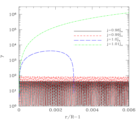
Figure 1: Dependence of the Lorentz factor on the ratio $j/\bar{j}_{\ast}$ for a neutron star with $M=1.4M_{\odot}$, $R=10\ \mathrm{km}$, $P=0.1s$, $\chi=30^{\circ}$, $B_{0}=1.0\times 10^{12}\mathrm{G}$, $\theta_{\ast}=0^{\circ}$, $\Theta_{0}=2^{\circ}$, and $\gamma_{\ast}=1.01$.

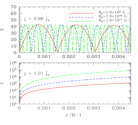
Figure 2: Lorentz factor dependence on the intensity of the magnetic field for a neutron star with $M=1.4M_{\odot}$, $R=10\ \mathrm{km}$, $P=0.1s$, $\chi=30^{\circ}$, $\theta_{\ast}=0^{\circ}$, $\Theta_{0}=2^{\circ}$, $\gamma_{\ast}=1.01$. Top panel: $j=0.98\bar{j}_{\ast}$. Bottom panel: $j=1.01\bar{j}_{\ast}$.

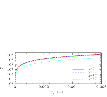
Figure 3: Lorentz factor dependence on the inclination angle $\chi$ for a neutron star with $M=1.4M_{\odot}$, $R=10\ \mathrm{km}$, and $P=0.1s$, $j=1.01\bar{j}_{\ast}$, $\theta_{\ast}=0^{\circ}$, $\Theta_{0}=2^{\circ}$, $\gamma_{\ast}=1.01$, and $B_{0}=1.0\times 10^{12}\mathrm{G}$. The Lorentz factor decreases for larger inclination angles.

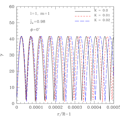
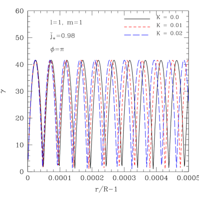
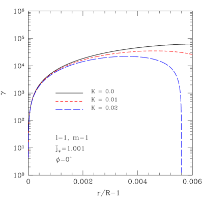
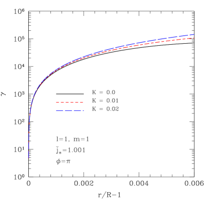
Figure 4: Lorentz factor dependence on the normalized amplitude of the stellar oscillations $K$ for the mode of oscillations $(l,m)=(1,1)$ with $\theta_{\ast}=2^{\circ}$, $\Theta_{0}=3^{\circ}$,$\gamma_{\ast}=1.015$, and $B_{0}=1.0\times 10^{12}\mathrm{G}$. The two top panels correspond to the case $j=0.98\bar{j}_{\ast}$, while the two bottom panels correspond to the case $j=1.001\bar{j}_{\ast}$. The left panels show the solution for $\phi=0$, the right panels for $\phi=\pi$.

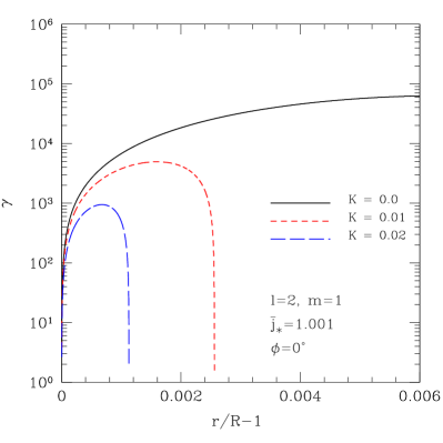
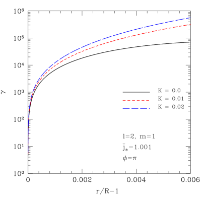
Figure 5: Lorentz factor dependence on the normalized amplitude of the stellar oscillations $K$ for the mode of oscillations $(l,m)=(2,1)$ with $\theta_{\ast}=2^{\circ}$, $\Theta_{0}=3^{\circ}$,$\gamma_{\ast}=1.015$, and $B_{0}=1.0\times 10^{12}\mathrm{G}$. The two panels correspond to the case $j=1.001\bar{j}_{\ast}$. The left panel shows the solution for $\phi=0$, and the right panel for $\phi=\pi$.

Fig. 1 reports the Lorentz factor as a function of the normalized radial coordinate $r/R-1$ for different values of the ratio $j/\bar{j}_{\ast}$. Fig. 1 essentially confirms the results of Sakai & Shibata (2003), which were originally predicted by Mestel et al. (1985), namely the existence of two different acceleration regimes. When $j<\bar{j}$, small values of the velocity $v$ can make the right-hand side of Eq. (8) positive, thus producing an increasing potential and an increasing Lorentz factor. As soon as the velocity reaches a critical value, given by the initial ratio $j/\bar{j}$, the right-hand side of Eq. (8) becomes negative and the potential, as well as the velocity, starts to decrease. As a result, the case $j<\bar{j}$ is responsible for the occurrence of an oscillatory regime, with the oscillation frequency (in the spatial domain) that is strongly dependent on the ratio $j/\bar{j}_{\ast}$. As shown by Mestel et al. (1985) and Shibata (1997), this situation corresponds to the case where the effective charge density $\rho-\rho_{\rm GJ,rot}$ changes sign. When $\rho-\rho_{\rm GJ,rot}>0$, the electron flow decelerates to increase the charge density; in contrast, when $\rho-\rho_{\rm GJ,rot}<0$, the flow accelerates to reduce the charge density. A rather different behavior is instead encountered when $j>\bar{j}$. In this case, the effective charge density is always negative, the right hand side of Eq. (8) is always positive, and the potential as well as the velocity can only grow.

Sakai & Shibata (2003) erroneously attributed the abrupt interruption of the oscillatory pattern, which is manifested by some models (see the bottom panel of their Fig. 1), to a purely general relativistic effect. In contrast and as we have verified, this effect is purely numerical and caused by $v^{2}$ possibly becoming negative during the integration of the system of equations Eqs. (8)-(9). For instance, this is also true for the long-dashed blue curve in Fig. 1, where the Lorentz factor decays to unity at $r/R-1\approx 0.003$ after having reached a value of $\gamma_{max}\sim 4100$. The pathology of the ODE system that we have demonstrated could not be solved even when resorting to stiff solvers. As a result, the behavior of the Lorentz factor after $v^{2}$ becomes negative cannot be trusted and is not reported in our figures. We also note that a value of $r/R-1=0.006$ corresponds to a distance of $60\ m$ above the star surface, which is smaller than the radius of the polar cap $r_{\rm pc}\approx R\leavevmode\nobreak\ \Theta_{0}\approx 350\ m$ as inferred by the polar cap model of Ruderman & Sutherland (1975).

On the other hand, Fig.2 illustrates the dependence of the Lorentz factor of the accelerated particles on the intensity of the magnetic field. We note that both the accelerating electric field $E_{\|}$ and the difference $\rho-\rho_{\rm GJ,rot}$ are directly proportional to the magnetic field (See Eq. (56) by Muslimov & Tsygan 1992). Therefore, if $j>\bar{j}_{\ast}$, corresponding to the case when the effective charge density is always negative, the Lorentz factor increases with the magnetic field, as shown in the bottom panel of Fig.2. On the other hand, if $j<\bar{j}_{\ast}$, corresponding to the case when the effective charge density changes sign, the charge density jump $|\rho-\rho_{\rm GJ,rot}|$ increases with the magnetic field, producing a pattern with a higher frequency of oscillation (See Eq. (23) by Shibata 1997). This effect is reported in the top panel of Fig.2.

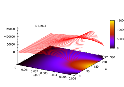
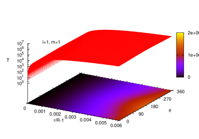
Figure 6: Lorentz factor as a function of radial distance and azimuthal angle $\phi$ for a model with stellar oscillations $K=0.02$, $(l,m)=(1,1)$, $\theta_{\ast}=2^{\circ}$, $\Theta_{0}=3^{\circ}$,$\gamma_{\ast}=1.015$, and $B_{0}=1.0\times 10^{12}\mathrm{G}$. Left panel: $j=1.001\bar{j}_{\ast}$. Right panel: $j=1.01\bar{j}_{\ast}$.

The dependence of the Lorentz factor on the inclination angle $\chi$ is shown in Fig.3. When $j<\bar{j}_{\ast}$, namely when the oscillatory pattern is produced, the Lorentz factor is insignificantly affected by variations in $\chi$ and the results are not reported here. In contrast, when $j>\bar{j}_{\ast}$, the results are more interesting and show that smaller Lorentz factors are obtained for larger inclination angles $\chi$, although this effect becomes significant only for very inclined configurations.

In a second series of calculations, we have considered the effects of stellar oscillations on the Lorentz-factor of the accelerated particles by adopting the prescription given in Eq. (2.2). Figures 4 and  5 show the solutions for the modes of oscillations $(l,m)=(1,1)$ and $(2,1)$, respectively. As is apparent from the two top panels of Fig. 4, the presence of stellar oscillations does not affect the amplitude of the Lorentz factor of the particle for $j=0.98\bar{j}_{\ast}$ and $(l,m)=(1,1)$. On the other hand, the frequency of the velocity oscillation is smaller for larger $K$ at $\phi=0^{\circ}$ (left-top panel), while it is larger for larger $K$ at $\phi=180^{\circ}$ (right-top-panel). As long as the velocity of oscillations for the considered modes is proportional to $\cos\phi$, the effect will be the opposite when $\cos\phi$ changes sign. The same qualitative behavior was also encountered for the mode $(l,m)=(2,1)$, and we conclude that it is typical of the case $j/\bar{j}_{\ast}<1$.

The case $j/\bar{j}_{\ast}\geq 1$ is reported in the two bottom panels of Fig. 4 for the mode $(l,m)=(1,1)$ and in Fig. 5 for the mode $(l,m)=(2,1)$, and illustrate that star oscillations can significantly affect the Lorentz factor. We note that the influence of the stellar oscillations on the acceleration of the particle strongly depends on the azimuthal angle $\phi$. In particular, owing to the modulation produced by the term $\cos\phi$, larger oscillation amplitudes $K$ become responsible for a net decelerating effect at angles $\phi\sim 0$, while they produce a net accelerating effect at angles $\phi\sim\pi$. Moreover, a strong dependence on the ratio $j/\bar{j}_{\ast}$ is also encountered, as is clearly evident from the two panels of Fig. 6, which show the modulation of the Lorentz factor with the angle $\phi$ for the mode $(l,m)=(1,1)$ in a representative model with $K=0.02$. The left panel refers to the case $j/\bar{j}_{\ast}=1.001$, while the right panel has $j/\bar{j}_{\ast}=1.01$. Interestingly, Morozova et al. (2010) found that the oscillation modes with $m=1$ considerably increase the electromagnetic energy losses from the polar cap region of the neutron star, losses that can be several times larger than in the case when no oscillations are present. A more efficient particle acceleration typically corresponds to higher energy losses from the neutron star magnetosphere (Osmanov & Rieger 2009). As a result, we conclude that, at least for the modes $(l,m)=(1,1)$ and $(l,m)=(2,1)$ that we have considered here, larger oscillation amplitudes at the stellar surface may be responsible for both stronger accelerations and higher luminosities, provided that the current density in the magnetosphere is higher than the Goldreich-Julian current density.

At least in the case of small inclination angles, a noticeable influence of stellar oscillations on the conditions for particle acceleration can be intuitively understood as follows. The acceleration of charged particles extracted from the surface of the pulsar in the polar cap region is determined by the electric field, which is generated by the combined effect of strong magnetic fields and the motion of the star surface. When stellar oscillations are added to the pure rigid rotation, a given velocity distribution at the star surface is produced. The rotation velocity in the polar cap region is proportional to the small polar angle $\theta$, is exactly equal to zero on the axis of rotation, and increases with distance away from the axis. In contrast, the velocity of oscillations, which is given by Eq. (18), in the case $m=1$ does not depend on the small polar angle $\theta$ and is effectively constant across the polar cap region of the star. This explains why for these modes even small oscillation velocities may have a noticeable effect on the accelerating component of the electric field.

4 CONCLUSIONS

By numerically solving the relativistic electrodynamics equations in the stationary regime of a space-charge-limited-flow accelerator, we have computed the Lorentz factor of electrons accelerated in the polar cap region of a rotating and oscillating pulsar magnetosphere. Our results confirm some of the fundamental findings of Sakai & Shibata (2003), namely the existence of two different regimes: an oscillatory one, which is produced for sub-GJ current density configurations, ($j/\bar{j}_{\ast}<1$) and does not produce an efficient acceleration, and a truly accelerating one, which is produced for super-GJ current density configurations ($j/\bar{j}_{\ast}>1$). We have also clarified the numerical origin of a stopping effect on the velocity of the electron, which has nothing to do with general relativistic effects. Stellar oscillations, on the other hand, can affect both the absolute value of the Lorentz factor gained by the electron and the frequency of the oscillatory patterns, when the latter is present. Owing to the modulation produced by the term $\cos\phi$ in the equations, where $\phi$ is the azimuthal angle, the way in which each mode of oscillation affects the dynamics is different at different azimuthal positions on the polar cap surface, and, in particular, it follows the periodicity of $\cos\phi$. These results are overall consistent with those obtained by Morozova et al. (2010), who showed that oscillations are responsible for an extra term in the total energy losses from the system, because the electromagnetic energy losses are determined by the integrated absolute value of the current, flowing in the magnetosphere. At least for the modes $(l,m)=(1,1)$ and $(l,m)=(2,1)$, larger oscillation amplitudes at the star surface may produce both higher accelerations and higher luminosities, provided that the magnetosphere has a super-GJ current density configuration. However, these results also suggest that pulsar oscillations may become responsible for a significant asymmetry in the pulse profile, which will depend on the orientation of the oscillations with respect to the pulsar magnetic field.

Finally, we stress that some recent investigations have tried to connect the models of stellar oscillations with the observational data available for pulsars (Rosen & Clemens 2008; Rosen & Demorest 2011; Rosen et al. 2011). The scenario that is emerging from these studies is that the presence of stellar oscillations creates different kinds of ”noise” in the clock-like picture of pulses, i.e. changes in the pulse shape, changes in the spin-down rate, and the switching between different regimes of pulsar emission. van Leeuwen & Timokhin (2012), in particular, revisited the issue of drifting subpulses in the pulsar profiles, reaching the important conclusion that the rate of subpulse drift is proportional to the latitudinal derivative of the scalar potential across the pulsar polar cap and not to the absolute value of the scalar potential, as had been generally assumed. This provides a wide range of opportunities for comparing the observational data on pulsar profiles with the results presented here and in our previous investigations of oscillating magnetopsheres. Stellar oscillations, indeed, affect the scalar potential in the polar cap region and are expected to have a significant effect on the character of the subpulse drift. We plan to devote our future research to a closer analysis of the observational aspects of these ideas.

Appendix A Extended geometrized system of units

We recall that the definition of geometric units of time and lengths is obtained by setting the speed of light $c$ and the gravitational constant $G$ to pure numbers. This implies that seconds and grams of the $\rm{cgs}$ system can be written as

$$1{\rm s} = 2.997924{\times}10^{10}\,\left(\frac{1}{c}\right)\,\rm{cm}\,$$ (26)

$$1\rm{g} = 7.424157{\times}10^{-29}\,\left(\frac{c^{2}}{G}\right)\,\rm{cm}\,.$$ (27)

Within this general setup, a convenient unit of space is still required. The $\rm{cm}$ is of course a bad choice in a gravitational framework and the gravitational radius $r_{g}=GM/c^{2}$ is instead chosen. In order for this new unit to be more convenient than the centimeter, the mass $M$ of the system has to be sufficiently high. From the physical value of the solar mass and Eq. (27), we find the relations between the cgs units and the new unit of length $r_{g}$

$${}_{1}\rm{cm} = 6.772289{\times}10^{-6}\,\left(\frac{M_{\odot}}{M}\right)\,r_{g}\,,$$ (28)

$$1\rm{s} = 2.030281{\times}10^{5}\,\left(\frac{1}{c}\right)\left(\frac{M_{\odot}}{M}\right)\,r_{g}\,,$$ (29)

$$1\rm{g} = 5.027854{\times}10^{-34}\,\left(\frac{c^{2}}{G}\right)\left(\frac{M_{\odot}}{M}\right)\,r_{g}\,.$$ (30)

In the traditional geometrized system $c$ and $G$ are set equal to unity. The equations Eqs. (28)-(30) allow us to perform the geometrization of any dynamical quantities. Quantities involving the charge, on the other hand, are naturally geometrized within the Gauss system of units, which we adopt here in addition to the choice $c=G=1$. In Gauss units, the unit of measure of the magnetic induction, the Gauss G, is given by

$$1G=\rm{g}^{1/2}\rm{cm}^{-1/2}\rm{s}^{-1}\ ,$$ (31)

which, by virtue of (28)-(30), provides

$$B_{\rm{geo}}=4.2439\times 10^{-20}\left(\frac{M}{M_{\odot}}\right)B_{\rm{G}}\ ,$$ (32)

where $B_{\rm{G}}$ and $B_{\rm{geo}}$ are the pure numbers expressing the intensity of the magnetic field in Gauss units and the geometrized system, respectively. We note that in these units the charge-to-mass ratio is a pure number, and, in the case of electrons, is given by

$$\frac{e}{m_{e}}=2.0425\times 10^{21}\ .$$ (33)

References

- Abdikamalov et al. (2009) Abdikamalov, E. B., Ahmedov, B. J., & Miller, J. C. 2009, Mon. Not. R. Astron. Soc., 395, 443
- Arons & Scharlemann (1979) Arons J., Scharlemann E. T., 1979, Astrophys. J., 231, 854
- Barzilay (2011) Barzilay, Y. 2011, Astrop. J., 732, 123
- Becker (2009) Becker, W., ed. 2009, Astrophysics and Space Science Library, Vol. 357, Neutron Stars and Pulsars
- Beskin (2010) Beskin V. S., 2010, MHD Flows in Compact Astrophysical Objects: Accretion, Winds and Jets. Springer-Verlag, Berlin
- Cheng & Ruderman (1980) Cheng, A. F. & Ruderman, M. A. 1980, Astrop. J., 235, 576
- Contopoulos et al. (1999) Contopoulos I., Kazanas D., Fendt C., 1999, Astrophys. J., 511, 351
- Daugherty & Harding (1982) Daugherty, J. K. & Harding, A. K. 1982, Astrop. J., 252, 337
- Fawley et al. (1977) Fawley, W. M., Arons, J., & Scharlemann, E. T. 1977, Astrop. J., 217, 227
- Fitzpatrick & Mestel (1988) Fitzpatrick, R. & Mestel, L. 1988, Mon. Not. R. Astron. Soc., 232, 277
- Ginzburg & Ozernoi (1965) Ginzburg, V. L. & Ozernoi, L. M. 1965, Soviet Phys.-JETP, 20, 689
- Goldreich & Julian (1969) Goldreich, P. & Julian, W. H. 1969, Astrophys. J., 157, 869
- Gruzinov (2005) Gruzinov, A. 2005, Phys. Rev. Lett., 94, 021101
- Harding & Muslimov (1998) Harding, A. K. & Muslimov, A. G. 1998, Astrop. J., 508, 328
- Hartle & Thorne (1968) Hartle, J. B. & Thorne, K. S. 1968, Astrop. J., 153, 807
- Kalapotharakos et al. (2011) Kalapotharakos, C., Kazanas, D., Harding, A., & Contopoulos, I. 2011, ArXiv e-prints
- McDermott et al. (1984) McDermott, P. N., Savedoff, M. P., van Horn, H. M., Zweibel, E. G., & Hansen, C. J. 1984, ApJ, 281, 746
- Mestel (1981) Mestel, L. 1981, in Sieber W., Wielebinski R., eds, Proc. IAU Symp. 95, Pulsars. Reidel, Dordrecht, p.9
- Mestel et al. (1985) Mestel, L., Robertson, J. A., Wang, Y.-M., & Westfold, K. C. 1985, Mon. Not. R. Astron. Soc., 217, 443
- Michel (1991) Michel, F. C. 1991, Theory of Neutron Star Magnetospheres (Chicago: Univ. Chicago Press)
- Morozova et al. (2008) Morozova, V. S., Ahmedov, B. J., & Kagramanova, V. G. 2008, Astrophys. J., 684, 1359
- Morozova et al. (2010) Morozova, V. S., Ahmedov, B. J. & Zanotti, O. 2010, Mon. Not. R. Astron. Soc., 408, 490
- Morozova et al. (2012) Morozova, V. S., Ahmedov, B. J., & Zanotti, O. 2012, Mon. Not. R. Astron. Soc., 419, 2147
- Muslimov & Tsygan (1986) Muslimov, A. G. & Tsygan, A. I. 1986, Ap&SS, 120, 27
- Muslimov & Harding (1997) Muslimov, A. & Harding, A. K. 1997, Astrophys. J., 485, 735
- Muslimov & Tsygan (1992) Muslimov, A. G. & Tsygan, A. I. 1992, Mon. Not. R. Astron. Soc., 255, 61
- Osmanov & Rieger (2009) Osmanov, Z. & Rieger, F. M. 2009, Astron. Astrophys., 502, 15
- Rezzolla et al. (2001) Rezzolla, L., Ahmedov, B. J., & Miller, J. C. 2001, Mon. Not. R. Astron. Soc., 322, 723
- Rezzolla & Ahmedov (2004) Rezzolla, L. & Ahmedov, B. 2004, Mon. Not. R. Astron. Soc., 352, 1161
- Rosen & Clemens (2008) Rosen R., Clemens J. C., 2008, Astrophys. J., 680, 671
- Rosen & Demorest (2011) Rosen R., Demorest P., 2011, Astrophys. J., 728, 156
- Rosen et al. (2011) Rosen R., McLaughlin M. A., Thompson S. E., 2011, Astrophys. J., 728, L19
- Ruderman & Sutherland (1975) Ruderman M. A., Sutherland P. G., 1975, Astrophys. J., 196, 51
- Sakai & Shibata (2003) Sakai, N. & Shibata, S. 2003, Astrophys. J., 584, 427
- Scharlemann et al. (1978) Scharlemann, E. T., Arons, J., & Fawley, W. M. 1978, Astrop. J., 222, 297
- Shibata (1997) Shibata, S. 1997, Mon. Not. R. Astron. Soc., 287, 262
- Steiner & Watts (2009) Steiner A. W., Watts A. L., 2009, Phys. Rev. Lett., 103, 181101
- Sturrock (1971) Sturrock, P. A. 1971, Astrophys. J., 164, 529
- Timokhin et al. (2000) Timokhin, A. N., Bisnovatyi-Kogan, G. S., & Spruit, H. C. 2000, Mon. Not. R. Astron. Soc., 316, 734
- Timokhin (2007) Timokhin, A. N. 2007, Astropys. Space Sci., 308, 345
- Timokhin et al. (2008) Timokhin, A. N., Eichler, D., & Lyubarsky, Y. 2008, Astrop. J., 680, 1398
- Unno et al. (1989) Unno, W., Osaki, Y., Ando, H., Saio, H. & Shibahashi H. 1989, Nonradial Oscillations of Stars. Univ. Tokyo Press, Tokyo
- van Leeuwen & Timokhin (2012) van Leeuwen, J. & Timokhin, A. N. 2012, ArXiv e-prints
- Wasserman & Shapiro (1983) Wasserman, I. & Shapiro, S. L. 1983, Astrophys. J., 265, 1036