Phase transitions in dipolar gases in optical lattices

Abstract

We investigate the phase diagrams of two-dimensional lattice dipole systems with variable geometry. For bipartite square and triangular lattices with tunable vertical sublattice separation, we find rich phase diagrams featuring a sequence of easy-plane magnetically ordered phases separated by incommensurate spin-wave states.

A recent breakthrough in the cooling of dipolar gases in optical lattices Chotia et al. , following a decade of intensive research Weinstein et al. (1998); Santos et al. (2000); Micheli et al. (2007); Ni et al. (2008); Deiglmayr et al. (2008); Aikawa et al. (2009); Baranov (2008); Lahaye et al. (2009), opens a door into the earlier inaccessible many-body physics of lattice systems with anisotropic long-range interaction. Although bulk crystalline dipolar systems are abundant in nature De’Bell et al. (2000); Lines and Glass (2001), their experimental investigation has been hindered by the extremely low temperatures required for the observation of ordering transitions Oja and Lounasmaa (1997) and the absence of continuously variable parameters. Recently, artificial two-dimensional dipolar systems, such as lithographically created nanomagnet arrays, have been realized Wang et al. (2006); Möller and Moessner (2006). However, it is the advent of optical lattices with tunable lattice structure containing ultracold dipolar gases, that creates numerous possibilities for studies of previously unexplored phase transitions – both classical and quantum – between ordered and disordered phases of this fundamental many-body system.

In this Article we analyze a series of magnetic phase transitions in a classical dipolar gas in deep optical lattices [square, Fig. 1 and triangular, Fig. 2] obtained from bipartite monolayer lattices by vertical separation, $z$, of the two sublattices. One way to realize such systems would be loading of ferromagnetic spinor Bose-Einstein mini-condensates in the nodes blu of a deep bilayer optical lattice created with the help of a painted potential technique Henderson et al. (2009), which would allow for high degree of control over the shapes of optical lattices and interlayer separation.

We find that, upon the variation of $z$, each system experiences a sequence of easy-plane magnetically ordered phases separated by incommensurate spin-wave states, which could be detected with the help of Bragg diffraction of light Weidemüller et al. (1995); Birkl et al. (1995); Corcovilos et al. (2010). The phase diagram for the square lattice on the $z-T$ plane is shown in Fig. 1. For sufficiently small separations $z\ll a$, where $a$ is lattice constant, we reproduce the earlier predicted Rozenbaum (1996); Gross et al. (2002) canted antiferromagnetic phase, $\mathrm{AF_{K}}$, with the ordering vector $\mathbf{K}$. For $z>a$, we find an antiferromagnetic phase, $\mathrm{AF_{M}}$, with larger unit cell and ordering wave vector at the M-point of the Brillouin zone of the bipartite lattice. For intermediate interlayer distances, we find a stable ferromagnetic phase (F), separated from the antiferromagnetic ones by incommensurate spin-wave states (ISW). At the critical temperature $T_{c}$, all of the ordered phases feature a degeneracy in the orientation of magnetization, characterized in Fig. 1 by angle $\theta$, or $\theta_{A}$ and $\theta_{B}$ for $\mathrm{AF_{M}}$.

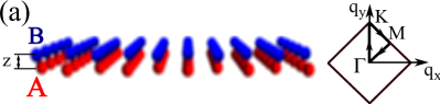
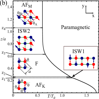
Figure 1: (color online) (a) Dipolar magnetic gas on a bipartite square optical lattice as seen along [0,1] axis and the first Brillouin zone. The two sublattices, $A$ and $B$, are vertically separated by the distance $z$. (b) Phase diagram of the dipolar gas: three commensurate phases ($\mathrm{AF_{K}}$, F, and $\mathrm{AF_{M}}$) separated by two incommensurate spin-wave phases (ISW1 and ISW2) with phase boundaries at $z_{1}=0.245a$, $z_{2}=0.262a$, $z_{3}=0.629a$ and $z_{4}=1.061a$, where $a$ is lattice constant, and $T_{0}=\mu_{0}\mu^{2}/4\pi a^{3}$.

Away from $T_{c}$, such a degeneracy is lifted, and Fig. 1 shows the optimal orientation of the order parameter for the low-temperature states. The structure of the intermediate incommensurate phases, ISW1 and ISW2 (Fig. 1) has also been established for $T\rightarrow T_{c}$, while their nature at low temperatures remains an open question.

We find that the phase diagram for the bipartite triangular lattice (which forms a honeycomb lattice when $z=0$) also contains a sequence of commensurate and incommensurate magnetic phases, Fig.2. For $z\ll a$, we find a helical phase with the ordering vector $\mathbf{K}$ ($\mathrm{H_{K}}$), which is specific for dipoles on a 2D honeycomb lattice Rozenbaum (1996) . A large vertical displacement of the two sublattices of the honeycomb lattice results in two weakly coupled triangular lattices, for which the ground state is ferromagnetic (F) Rozenbaum (1996). In between those two extremes lies an antiferromagnetic phase $\mathrm{AF_{M}}$ with the ordering vector $\mathbf{M}$ Mph , separated from the helical and ferromagnetic phases by parametric intervals, where the magnetization texture is incommensurate with the lattice.

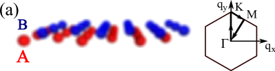
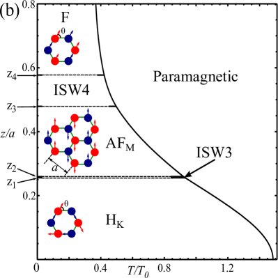
Figure 2: (a) Dipolar magnetic gas on a bipartite triangular optical lattice as seen along [0,1] axis and the first Brillouin zone. The two sublattices, A and B, are vertically shifted separated by the distance $z$ (at $z=0$, they form a honeycomb lattice). (b) Phase diagram of the dipolar gas: three commensurate phases ($\mathrm{H_{K}}$, $\mathrm{AF_{M}}$, and F) separated by two incommesurate spin-wave phases (ISW3 and ISW4) with phase boundaries at $z_{1}=0.256a$, $z_{2}=0.2600a$, $z_{3}=0.479a$ and $z_{c4}=0.577a$, where $a$ is lattice constant and $T_{0}=\mu_{0}\mu^{2}/4\pi a^{3}$.

To find phase diagrams in Figs. 1, 2, we consider an ensemble of classical magnetic dipoles $\mu\mathbf{s}_{i}$ ($|\mathbf{s}_{i}|^{2}=1$), placed on the A or B sites $\mathbf{r}_{i}^{n}$ ($n=A,B$) of the square (Fig. 1) or triangular (Fig. 2) lattices, with interaction energy

$$H=\frac{1}{2}\sum_{i\neq j}\sum_{\alpha,\beta=x,y,z} \sum_{n,n^{\prime}=A,B}J^{\alpha\beta}(\mathbf{r}_{i}^{n}-\mathbf{r}_{j}^{n^{\prime}})s^{\alpha}(\mathbf{r}_{i}^{n})s^{\beta}(\mathbf{r}_{j}^{n^{\prime}}),$$

$$J^{\alpha\beta}(\mathbf{r}) =\frac{\mu_{0}\mu^{2}}{4\pi r^{3}}\left(\delta_{\alpha\beta}-3\frac{r^{\alpha}r^{\beta}}{r^{2}}\right).$$ (1)

Here $\mu_{0}$ is the vacuum permeability. The Hamiltonian is invariant under the group $\mathcal{G}$ of simultaneous rotation of magnetic moments in the $xy$-plane and the lattice rotations through the angles $\pi/4$ for square and $\pi/3$ for triangular lattices.

In order to identify the thermodynamic average, $\langle\mathbf{s}(\mathbf{r}_{i}^{n})\rangle$ ($n=A,B$), of magnetization for various interlayer separations $z$, we apply the Landau theory and study the free energy in the vicinity of the transition temperature Palmer and Chalker (2000),

$$F=\frac{N}{2}\sum_{\mathbf{q}}\mathbf{S}^{\dagger}({\mathbf{q})}\left(3T\hat{\mathbbm{1}}+\hat{\mathrm{J}}(\mathbf{q})\right)\mathbf{S}(\mathbf{q})+F^{(m)}+...,$$ (2)

expressed in terms of a 6-vector

$$\mathbf{S(\mathbf{q})}^{\mathrm{T}}=(S_{A}^{x}(\mathbf{q}),S_{A}^{y}(\mathbf{q}),S_{A}^{z}(\mathbf{q}),S_{B}^{x}(\mathbf{q}),S_{B}^{y}(\mathbf{q}),S_{B}^{z}(\mathbf{q})),$$

where $S_{n}^{\alpha}(\mathbf{q})$ is the Fourier transform of the order parameter $\langle\mathbf{s}(\mathbf{r}_{i}^{n})\rangle$ of magnetic moments on A and B sublattices. In Eq. 2, $\hat{\mathbbm{1}}$ is a $6\times 6$ unit matrix, and $F^{(m)}$ incorporates higher-order invariants under the group $\mathcal{G}$ built using the order parameter ($m=4$ for square and $m=6$ for triangular lattices). A $6\times 6$ matrix $\hat{\mathrm{J}}$ has elements

$$J_{nn^{\prime}}^{\alpha\beta}(\mathbf{q})=(1/N)\sum_{ij}J^{\alpha\beta}(\mathbf{r}_{i}^{n}-\mathbf{r}_{j}^{n^{\prime}})e^{i\mathbf{q}\cdot(\mathbf{r}_{i}^{n}-\mathbf{r}_{j}^{n^{\prime}})},$$ (3)

where $N$ is the number of unit cells. For each wave vector $\mathbf{q}$, matrix $\hat{\mathrm{J}}$ has $6$ eigenvalues, $\lambda$, and $6$ eigenvectors, $\mathbf{V}(\mathbf{q})$. The lowest negative eigenvalue $\lambda_{0}(\mathbf{q}_{0})$ found among $\lambda_{\gamma}(\mathbf{q})$ by varying wave vector $\mathbf{q}$ over the Brillouin zone determines the polarizations $\mathbf{V}(\mathbf{q}_{0})$ and the wave vector $\mathbf{q}_{0}$ of the most favorable magnetic ordering and the transition temperature

$$T_{c}=-\frac{1}{3}\min_{\gamma,\mathbf{q}}(\lambda_{\gamma}(\mathbf{q}))\equiv\frac{1}{3}|\lambda_{0}(\mathbf{q}_{0})|.$$ (4)

In Fig. 3, we show plots for $\lambda_{\gamma}(\mathbf{q})$ for the square bipartite lattice with various vertical A-B sublattice separations. For $0\leq z\leq z_{1}$, where $z_{1}=0.245a$ ($a$ is lattice constant) $\mathbf{q}_{0}$ coincides with one of $\mathbf{K}$-points of the Brillouin zone as shown in Fig.3 (a)-(b). This corresponds to the $\mathrm{AF_{K}}$ phase (Fig. 1) with the order parameter

$$\langle\mathbf{s}(\mathbf{r}_{i}^{n})\rangle\propto(\cos(\mathbf{K}\cdot\mathbf{r}_{i}^{n}+\theta),p\sin(\mathbf{K}\cdot\mathbf{r}_{i}^{n}+\theta)),$$ (5)

where $p=\pm 1$ for $n=A/B$, and $\theta$ is a constant. In Eq. (2), the degeneracy in $\theta$ is lifted by the higher-order terms $F^{(m)}$ appearing after taking into account thermal fluctuations. As $z$ increases from $z_{1}$ to $z_{2}=0.262a$, $\mathbf{q}_{0}$ continuously moves from $\mathbf{K}$- to $\Gamma$- point (Fig.4 (a)), and the corresponding eigenvector $\mathbf{V}_{0}(\mathbf{q}_{0})$ determines the magnetization texture

$$\langle\mathbf{s}(\mathbf{r}_{i}^{n})\rangle\propto\hat{\mathbf{z}}\times\mathbf{q}_{0}\cos(\mathbf{q}_{0}\cdot\mathbf{r}_{i}^{n})$$ (6)

of the incommensurate phase ISW1 illustrated in Fig. 1 (b), where $\hat{z}$ is the unit vector perpendicular to the plane of the lattice and $\mathbf{q}_{0}=(q_{0},0)$. For $z_{2}\leq z\leq z_{3}$, where $z_{3}=0.629a$, $\mathbf{q}_{0}$ lies at $\Gamma$-point (Fig. 3 (d)), which corresponds to the easy-plane ferromagnetic (F) ordering. As $z$ increases from $z_{3}$ to $z_{4}=1.061a$, $\mathbf{q}_{0}$ continuously moves from $\Gamma$- to $M$-point (Fig. 4 (b)), which determines the incommensurate spin-wave state ISW2 and the order parameter given by Eq. (6) with $\mathbf{q}_{0}=(1/\sqrt{2})(q_{0},q_{0})$. For $z\geq z_{4}$, $\mathbf{q}_{0}$ is at one of $M$-points (Fig. 3 (f)) giving rise to the phase $\mathrm{AF_{M}}$, which can be viewed as two weakly coupled "$\mathrm{AF_{K}}$" phases on each of two square sublattice. The form of the order parameter in each of the commensurate phases is given in Table 1.

The phase diagram for the bipartite triangular lattice (Fig. 2 (b) with order parameters listed in Table 1) is somewhat similar to that for the square bipartite lattice. For $0\leq z\leq z_{1}$, where $z_{1}=0.256a$, we find that $\mathbf{q}_{0}$ is at one of the $\mathbf{K}$-points. This corresponds to the helical $\mathrm{H_{K}}$ phase with the order parameter given by Eq. (5), where vector $\mathbf{K}$ is at the corner of the hexagonal Brillouin zone of triangular lattice (Fig. 2 (a)). Such a phase has been discussed in relation with a dipolar gas in a planar honeycomb lattice Rozenbaum (1996). For $z_{1}\leq z\leq z_{2}$, where $z_{2}=0.260a$, $\mathbf{q}_{0}$ continuously shifts from $\mathbf{K}$ to $\mathbf{M}$-point giving rise to the incommensurate phase ISW3 with magnetization texture

$$\langle\mathbf{s}(\mathbf{r}_{i}^{n})\rangle\propto(-\sin(\mathbf{q}_{0}\cdot\mathbf{r}_{i}^{n}),pa_{y}\cos(\mathbf{q}_{0}\cdot\mathbf{r}_{i}^{n}),a_{z}\sin(\mathbf{q}_{0}\cdot\mathbf{r}_{i}^{n})),$$

where $0\leq a_{y}$ and $a_{z}\ll a_{y}$ are z-dependent, $\mathbf{q}_{0}=q_{0}(\mathbf{K}(1-c)+\mathbf{M}c)/|(\mathbf{K}(1-c)+\mathbf{M}c)|$ ($0\leq c\leq 1$). For $z_{2}\leq z\leq z_{3}$, where $z_{3}=0.479$, $\mathbf{q}_{0}$ lies at one of the M-points, which corresponds to the easy-plane antiferromagnetic phase $\mathrm{AF_{M}}$ shown in Fig. 2 (b) Mph . For $z_{3}\leq z\leq z_{4}$, where $z_{4}=0.577a$, $\mathbf{q}_{0}$ moves from $\mathbf{M}$- to $\Gamma$-points, which determines the incommensurate spin-wave state ISW4,

$$\langle\mathbf{s}(\mathbf{r}_{i}^{n})\rangle\propto(\sin(\mathbf{q}_{0}\cdot\mathbf{r}_{i}^{n}),\cos(\mathbf{q}_{0}\cdot\mathbf{r}_{i}^{n}))$$ (7)

with $\mathbf{q}_{0}=q_{0}\mathbf{M}/|\mathbf{M}|$. Finally, for $z\geq z_{4}$, $\mathbf{q}_{0}$ lies at $\Gamma$-point, which corresponds to an easy-plane ferromagnetic state. In the limit $z\rightarrow\infty$, this coincides with the ground state calculated for a dipolar magnet on a plane triangular lattice Rozenbaum (1996).

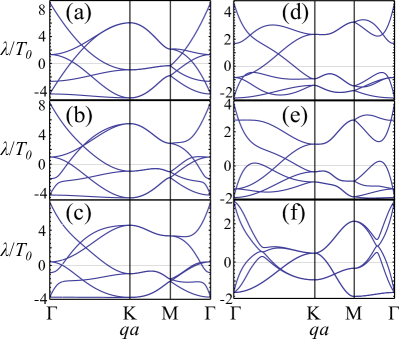
Figure 3: Eigenvalues, $\lambda_{i}(\mathbf{q})$, of the dipolar tensor, $J_{nn^{\prime}}^{\alpha\beta}$, for the square lattice as functions of the wave vector $\mathbf{q}$ along symmetric directions in the Brillouin zone (see Fig.1(a)) for a set of lattice displacements, $z$: (a) $z=0$; (b) $z=0.140a$; (c) $z=0.248a$; (d) $z=0.500a$; (e) $z=0.707a$; (f) $z=2.120a$.

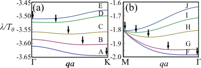
Figure 4: The minimal eigenvalues $\lambda_{0}$ vs. $\mathbf{q}$ along symmetric directions in the Brillouin zone for incommensurate phases: (a) ISW1 and (b) ISW2 for a representative set of $z$: (A) $z=0.245a$; (B) $z=0.250a$; (C) $z=0.255a$; (D) $z=0.260a$; (E) $z=0.262a$; (F) $z=0.629a$; (G) $z=0.651a$; (H) $z=0.743a$; (I) $z=0.849a$; (J) $z=1.061a$. Arrows show the positions of the minima, $\mathbf{q}_{0}$, of $\lambda$. The ordering vector, $\mathbf{q}_{0}$ continuously moves along the straight lines connecting the K- and $\Gamma$- points (a) and $\Gamma$- and M-points (b), as $z$ increases.

Table 1: Order parameter for each of the commensurate phases of a dipolar gas on bipartite square and triangular lattices.

Lattice	Phase	$\mathbf{S}\equiv\langle\mathbf{s}(\mathbf{r}_{i}^{n})\rangle/|\langle\mathbf{s}(\mathbf{r}_{i}^{n})\rangle|$	$\mathbf{q}_{0}$	$\theta_{0}$
Square	$\mathrm{AF_{K}}$	$(\cos(\mathbf{K}\cdot\mathbf{r}_{i}^{n}+\theta),p\sin(\mathbf{K}\cdot\mathbf{r}_{i}^{n}+\theta))$, $p=\pm 1$ for A/B	$\mathbf{K}=(0,\frac{\sqrt{2}\pi}{a})$	$\frac{\pi k}{2}$, $k\in\mathbb{Z}$
$n=A,B$	F	$(\cos\theta,\sin\theta)$	$0$	$\frac{\pi k}{2}$, $k\in\mathbb{Z}$
	$\mathrm{AF_{M}}$	$(\cos(\mathbf{M}\cdot\mathbf{r}_{i}^{n}\pm\theta_{n}+\pi/4),\sin(\mathbf{M}\cdot\mathbf{r}_{i}^{n}\pm\theta_{n}+\pi/4))$ AB	$\mathbf{M}=(\frac{\sqrt{2}\pi}{2a},\frac{\sqrt{2}\pi}{2a})$	$\frac{\pi k}{2}$, $k\in\mathbb{Z}$
Triangular	$\mathrm{H_{K}}$	$(\cos(\mathbf{K}\cdot\mathbf{r}_{i}^{n}+\theta),p\sin(\mathbf{K}\cdot\mathbf{r}_{i}^{n}+\theta))$	$\mathbf{K}=(0,\frac{4\sqrt{3}\pi}{3a})$	$\frac{\pi k}{3}$, $k\in\mathbb{Z}$
$n=A,B$	$\mathrm{AF_{M}}$	$(\sin(\mathbf{M}\cdot\mathbf{r}_{i}^{n}),\cos(\mathbf{M}\cdot\mathbf{r}_{i}^{n}))$	$\mathbf{M}=(\frac{2\pi}{\sqrt{3}a},0)$	—
	F	$(\cos\theta,\sin\theta)$	$0$	$\frac{\pi k}{3}$, $k\in\mathbb{Z}$

The above analysis of magnetic phases of dipolar gases on square and triangular bipartite lattices, limited to the quadratic terms in the Landau theory, is formally valid at $T\rightarrow T_{c}$. To extend the phase diagrams in Figs. 1 and 2 to low temperatures, we investigate the stability of the ordering patterns described in Table 1 near $T=0$ using the linear spin-wave theory Palmer and Chalker (2000). That is, we expand the interaction energy in small deviations of on-site magnetic moments from the ground-state value $\langle\mathbf{s}(\mathbf{r}_{i}^{k})\rangle$,

$$E=E(\mathbf{S})+\frac{N_{M}}{2}\sum_{\mathbf{q}}\mathbf{\sigma}^{\dagger}(\mathbf{q})\hat{\mathrm{A}}(\mathbf{q})\mathbf{\sigma}(\mathbf{q}).$$ (8)

Such deviations have to respect the constraint $|\mathbf{s}(\mathbf{r}_{i}^{k})|^{2}=1$ and can be parametrized as

$$\mathbf{s}(\mathbf{r}_{i}^{k})=\langle\mathbf{s}(\mathbf{r}_{i}^{k})\rangle+\hat{\mathbf{z}}\sigma_{z}(\mathbf{r}_{i}^{k})+(\hat{\mathbf{z}}\times\langle\mathbf{s}(\mathbf{r}_{i}^{k}))\rangle\sigma_{||}(\mathbf{r}_{i}^{k})$$

$$-(1/2)\langle\mathbf{s}(\mathbf{r}_{i}^{k})\rangle[(\sigma_{||}(\mathbf{r}_{i}^{k}))^{2}+(\sigma_{z}(\mathbf{r}_{i}^{k}))^{2}].$$

Here we use the Fourier transform, $\mathbf{\sigma}(\mathbf{q})^{\mathrm{T}}=(\sigma^{1}_{||}(\mathbf{q}),\sigma^{1}_{z}(\mathbf{q}),...,\sigma^{k}_{||}(\mathbf{q}),\sigma^{k}_{z}(\mathbf{q}),...)$ of $\sigma_{\alpha}(\mathbf{r}_{i}^{k})$, index $k=1,...,M$ labels sites within the magnetic unit cell of a commensurate phase, so that the Fourier transform of $\langle\mathbf{s}(\mathbf{r}_{i}^{k})\rangle$ is $\mathbf{S}_{k}(\mathbf{q})=\mathbf{S}_{k}\delta(\mathbf{q})$ and $N_{M}$ is the number of magnetic unit cells. The $2M\times 2M$ matrix $\hat{\mathrm{A}}(\mathbf{q})$ has elements $A_{kk^{\prime}}^{||,||}(\mathbf{q})=\sum_{\alpha\beta}(\hat{\mathbf{z}}\times\mathbf{S}_{k})^{\alpha}J_{kk^{\prime}}^{\alpha\beta}(\mathbf{q})(\hat{\mathbf{z}}\times\mathbf{S}_{k^{\prime}})^{\beta}+f(0)$, $A_{kk^{\prime}}^{||,z}(\mathbf{q})=\sum_{\alpha}(\hat{\mathbf{z}}\times\mathbf{S}_{k})^{\alpha}J_{kk^{\prime}}^{\alpha z}(\mathbf{q})$, $A_{kk^{\prime}}^{z,||}(\mathbf{q})=\sum_{\beta}J_{kk^{\prime}}^{z\beta}(\mathbf{q})(\hat{\mathbf{z}}\times\mathbf{S}_{k^{\prime}})^{\beta}$, $A_{kk^{\prime}}^{zz}(\mathbf{q})=J_{kk^{\prime}}^{zz}(\mathbf{q})+f(0)$, where $f(0)=(-1/2)\sum_{\alpha\beta}S_{k}^{\alpha}J_{kk^{\prime}}^{\alpha\beta}(0)S_{k^{\prime}}^{\beta}$. We find that all eigenvalues of $\hat{\mathrm{A}}(\mathbf{q})$ are positive for $\mathbf{q}\neq 0$ within the same intervals $z_{i}<z<z_{i+1}$ , whereas at the edges of the intervals, the lowest eigenvalue of $\hat{\mathrm{A}}(\mathbf{q})$ acquires negative values reflecting a tendency towards incommensurate textures.

For most of the phases in Table 1, the interaction is degenerate in angle $\theta$ (Figs. 1 and 2). This degeneracy is lifted Prakash and Henley (1990) by thermal fluctuations leading to the higher-order expansion terms in the Landau theory. To find, at least for $T\ll T_{c}$, such symmetry breaking contributions, we take into account fluctuations $\mathbf{\sigma}(\mathbf{q})$ of the order parameter following Prakash and Henley (1990) and calculate the entropy part of the free energy

$$\delta F_{s}=-T\ln\prod_{\mathbf{q}}\int D\mathbf{\sigma}(\mathbf{q})\exp[-\frac{1}{2T}\mathbf{\sigma}^{\dagger}(\mathbf{q})\hat{\mathrm{A}}(\mathbf{q})\mathbf{\sigma}(\mathbf{q})]$$

$$\approx\frac{N_{M}T}{2}\sum_{\mathbf{q}\in BZ}\ln(\det\hat{\mathrm{A}}(\mathbf{q})).$$ (9)

We evaluate the dominant contribution from the fluctuations lifting the degeneracy with respect to angle $\theta$:

$$\delta F_{s}\approx TA_{0}-TA_{1}\cos(m\theta),A_{0},A_{1}>0,$$ (10)

where $m=4$ for square and $m=6$ for triangular lattice AB . This determines the optimal choice $\theta_{0}$ shown in Table 1. For $T\rightarrow T_{c}$, such entropy terms give rise to the crystalline anisotropy contribution $F^{(m)}\propto T_{c}|\mathbf{S}|^{m}\cos m\theta$ in Eq. (2).

For magnetic dipolar gases in deep bipartite (bilayer) square and triangular optical lattices, the predicted phase diagram may appear very much within the experimentally accessible range of controlled parameters. For deep optical lattices with $a\sim 1\mathrm{\mu m}$ and optical field trapping mini-condensates of $10^{3}$ spin-aligned ${}^{87}\mathrm{Rb}$ atoms per unit cell, we estimate $T_{c}\sim 50\mathrm{\mu K}$ in the phase diagram in Figs. 1 and 2. Moreover, as the electric and magnetic dipole interactions are mathematically equivalent, the phase diagram in Figs. 1 and 2 should be applicable to the electric dipolar systems, where we estimate $T_{c}\sim 100\mathrm{nK}$ for ferro- and antiferroelectric transitions in molecules with a dipole moment $d\sim 1\mathrm{D}$.

References

(1)
A. Chotia,
B. Neyenhuis,
S. A. Moses,
B. Yan,
J. P. Covey,
M. Foss-Feig,
A. M. Rey,
D. S. Jin, and
J. Ye,
arXiv:1110.4420 (2011).
Weinstein et al. (1998)
J. Weinstein,
R. deCarvalho,
T. Guillet,
B. Friedrich,
and J. Doyle,
Nature 395,
148 (1998).
Santos et al. (2000)
L. Santos,
G. V. Shlyapnikov,
P. Zoller, and
M. Lewenstein,
Phys. Rev. Lett. 85,
1791 (2000).
Micheli et al. (2007)
A. Micheli,
G. Pupillo,
H. P. Büchler,
and P. Zoller,
Phys. Rev. A 76,
043604 (2007).
Ni et al. (2008)
K.-K. Ni,
S. Ospelkaus,
M. H. G. de Miranda,
A. Pe’er,
B. Neyenhuis,
J. J. Zirbel,
S. Kotochigova,
P. S. Julienne,
D. S. Jin, and
J. Ye,
Science 322,
231 (2008).
Deiglmayr et al. (2008)
J. Deiglmayr,
A. Grochola,
M. Repp,
K. Mörtlbauer,
C. Glück,
J. Lange,
O. Dulieu,
R. Wester, and
M. Weidemüller,
Phys. Rev. Lett. 101,
133004 (2008).
Aikawa et al. (2009)
K. Aikawa,
D. Akamatsu,
J. Kobayashi,
M. Ueda,
T. Kishimoto,
and S. Inouye,
New J. Phys. 11,
055035 (2009).
Baranov (2008)
M. Baranov,
Phys. Rep. 464,
71 (2008).
Lahaye et al. (2009)
T. Lahaye,
C. Menotti,
L. Santos,
M. Lewenstein,
and T. Pfau,
Rep. Prog. Phys. 72,
126401 (2009).
De’Bell et al. (2000)
K. De’Bell,
A. B. MacIsaac,
and J. P.
Whitehead, Rev. Mod. Phys.
72, 225 (2000).
Lines and Glass (2001)
M. E. Lines and
A. M. Glass,
Principles and applications of ferroelectrics and
related materials (Oxford University Press,
2001).
Oja and Lounasmaa (1997)
A. S. Oja and
O. V. Lounasmaa,
Rev. Mod. Phys. 69,
1 (1997).
Wang et al. (2006)
R. F. Wang,
C. Nisoli,
R. S. Freitas,
J. Li,
W. McConville,
B. J. Cooley,
M. S. Lund,
N. Samarth,
C. Leighton,
V. H. Crespi,
et al., Nature
439, 303 (2006).
Möller and Moessner (2006)
G. Möller and
R. Moessner,
Phys. Rev. Lett. 96,
237202 (2006).
(15)
The presence of the trapping potential can have an important
effect on the ordering patterns discussed here because of light-induced
dipole-dipole interaction. However, this effect can be neglected for
blue-detuned lattices, where atoms are located in the nodes Zhang et al. (2002).
Henderson et al. (2009)
K. Henderson,
C. Ryu, and
C. MacCormick,
New J. Phys. 11,
043030 (2009).
Weidemüller et al. (1995)
M. Weidemüller,
A. Hemmerich,
A. Görlitz,
T. Esslinger,
and T. W.
Hänsch, Phys. Rev. Lett.
75, 4583 (1995).
Birkl et al. (1995)
G. Birkl,
M. Gatzke,
I. H. Deutsch,
S. L. Rolston,
and W. D.
Phillips, Phys. Rev. Lett.
75, 2823 (1995).
Corcovilos et al. (2010)
T. A. Corcovilos,
S. K. Baur,
J. M. Hitchcock,
E. J. Mueller,
and R. G. Hulet,
Phys. Rev. A 81,
013415 (2010).
Rozenbaum (1996)
V. M. Rozenbaum,
Phys. Rev. B 53,
6240 (1996).
Gross et al. (2002)
K. Gross,
C. P. Search,
H. Pu,
W. Zhang, and
P. Meystre,
Phys. Rev. A 66,
033603 (2002).
(22)
Similar phase has been recently predicted in Varney et al. (2011) for
an XY- spin model on a honeycomb lattice with next-to-nearest neighbors
interactiion.
Palmer and Chalker (2000)
S. E. Palmer and
J. T. Chalker,
Phys. Rev. B 62,
488 (2000).
(24)
For the phase of the dipolar gas in the square
lattice the interaction energy is degenerate in two parameters,
and (see Fig. 1). This degeneracy is lifted by
thermal fluctuations leading to , and the anisotropy term of the Landau theory
is . The
optimal choice of these degeneracy parameters is given in Table
1.
Prakash and Henley (1990)
S. Prakash and
C. L. Henley,
Phys. Rev. B 42,
6574 (1990).
Zhang et al. (2002)
W. Zhang,
H. Pu,
C. Search, and
P. Meystre,
Phys. Rev. Lett. 88,
060401 (2002).
Varney et al. (2011)
C. N. Varney,
K. Sun,
V. Galitski, and
M. Rigol,
Phys. Rev. Lett. 107,
077201 (2011).