Coherent control of atomic spin currents in a double well

Abstract

We propose a method for controlling the atomic currents of a two-component Bose-Einstein condensate in a double well by applying an external field to the atoms in one of the potential wells. We study the ground-state properties of the system and show that the directions of spin currents and net-particle tunneling can be manipulated by adiabatically varying the coupling strength between the atoms and the field. This system can be used for studying spin and tunneling phenomena across a wide range of interaction parameters. In addition, spin-squeezed states can be generated. It is useful for quantum information processing and quantum metrology.

I Introduction

Spin and tunneling phenomena are of fundamental interests in understanding quantum behaviors of particles. They are also important in the applications using solid-state devices such as sensors and data storage Fert . In addition, manipulation of the quantum state of a single spin is essential in implementing quantum information processing Nielsen .

Recently, the tunneling dynamics of ultracold atoms has been observed in a double well Albiez and optical lattices Folling , where the experimental parameters can be widely tuned. Moreover, high-fidelity single-spin detection of an atom has been realized in an optical lattice Bakr ; Weitenberg and atom-chip Volz , respectively. Such sophisticated techniques of manipulating ultracold atoms open up the possibilities for the study of intriguing quantum phenomena never possible before.

In this paper, we propose a method to control the tunneling dynamics of a two-component Bose-Einstein condensate (BEC) in a double well Ng by applying an external field to the atoms in one of the potential wells. In fact, the methods for controlling of tunneling in a double-well BEC have been suggested by driving the double-well potentials Holthaus and by applying a symmetry-breaking field MMolina , respectively. Besides, a number of methods for manipulating the atomic motions in an an optical lattice have been proposed such as using external fields for vibrational transitions between adjacent sites Forster , tilting the lattice potential DFrazer and periodic modulation of the lattice parameters Creffield .

Here we show that the spin and tunneling dynamics of atoms can be manipulated by adiabatically changing the coupling strength of the field. This approach can be used for studying the spin and tunneling related phenomena in a controllable manner. For example, the directions of “spin currents” such as parallel- and counter-flows can be controlled by appropriately adjusting the interaction parameters. Here the “spin currents” refer to the two atomic currents of a condensate of ⁸⁷Rb atoms with the two different hyperfine levels Harber . Apart from changing the internal states of atoms, the external field gives rise to net-particle tunneling. It is different to the situation of co-tunneling of the two component condensates in a double well Ng ; Kuklov in which the number difference of atoms between the wells is equal during the tunneling process.

In addition, the tunnel behaviors are totally different in the limits of weak and strong atomic interactions. In the regime of weak atomic interactions, the atoms smoothly tunnel through the other well. On the contrary, the discrete steps of tunneling are shown in the limit of strong atomic interactions. The coherent control of single-atom tunneling can thus be achieved. This method can be utilized for atomic transport.

Furthermore, we investigate the production of spin squeezing Kitagawa ; Wineland in this system. The occurrence of spin-squeezing can indicate multi-particle entanglement Sorensen . We show that spin-squeezed states can be dynamically generated by slowly changing the coupling strength of the field. This can be used for preparing entangled states and quantum metrology Esteve .

This paper is organized as follows: In Sec. II, we introduce the system of a two-component BEC in a double well, where the atoms in the left potential well are coupled to the laser field. In Sec. III, we study the ground-state properties of the system. In Sec. IV, we propose a method to adiabatically transfer the atoms to the other well. In Sec. V, we investigate the generation of multi-particle entanglement using this method. We provide a summary in Sec. VI. In the Appendix, we derive an effective Hamiltonian describing the coupling between the two internal states with the lasers.

II System

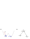
Figure 1: (Color online) (a) Schematic of a two-component Bose-Einstein condensate in a double well. An external field is applied to the atoms in the left potential well. (b) Energy levels for the atoms. The two internal states $|e\rangle$ and $|g\rangle$ are coupled via the upper state $|r\rangle$.

We consider a condensate of ⁸⁷Rb atoms with two hyperfine levels $|e\rangle=|F=2,m_{F}=1\rangle$ and $|g\rangle=|F=1,m_{F}=-1\rangle$ of the $5S_{1/2}$ ground state Harber confined in a symmetric double-well potential Ng . An external field is applied to the atoms in one of the potential wells. The schematic of the system is shown in Fig. 1(a). This system can be described by the total Hamiltonian $H_{\rm tot}=H_{0}+H_{1}$, where $H_{0}$ and $H_{1}$ are the Hamiltonians describing the external and internal degrees of atoms.

We adopt the two-mode approximation to describe the atoms in deep potential wells Ng . Since the scattering lengths of the different hyperfine states of ⁸⁷Rb are very similar Matthews , we assume that the intra- and inter-component interactions are nearly the same. The Hamiltonian $H_{0}$ can be written as ($\hbar=1$)

$$H_{0} = -J(e^{{\dagger}}_{L}e_{R}+e^{\dagger}_{R}e_{L}+g^{{\dagger}}_{L}g_{R}+g^{\dagger}_{R}g_{L})$$ (1)

$$+U[({n}_{eL}+n_{gL})^{2}+(n_{eR}+n_{gR})^{2}],$$

where $\alpha_{L}(\alpha_{R})$ and $n_{\alpha_{L}}(n_{\alpha_{R}})$ are annihilation operator of an atom and number operator in the left(right) potential well, for $\alpha=e,g$. The total number $N$ of atoms is conserved in this system. To ensure the validity of two-mode approximation, we assume that the trapping energy is much larger than the atomic interaction energy Milburn ; Holthaus , i.e., $\omega_{0}\gg{UN}$, where $\omega_{0}$ is the effective trapping frequency of the potential well.

We can make a rough estimation of the experimental parameters within the two-mode approximation. For ⁸⁷Rb, the scattering length $a$ is about 5 nm. We take the frequencies $\omega_{y}$ and $\omega_{z}$ of the transervse trapping potentials to be about $2\pi{\times}1$ kHz. Indeed, the barrier height and the separation between the two potential minima can be varied Maussang by appropriately splitting the potential. We consider that the barrier height $V_{b}$ can be tuned Maussang from $2\pi\times 50$ to $2\pi\times 250$ Hz and the separation $2x_{0}$ between two wells are 2 and 4 $\mu$m. The effective frequency $\omega_{0}=\sqrt{8V_{b}/(mx^{2}_{0})}$ Milburn is related to the barrier height $V_{b}$ and the separation $2x_{0}$. This gives the effective frequency $\omega_{0}$ ranging from $2\pi\times{220}$ to $2\pi\times{350}$ Hz, and the interaction strength $U$ ranges between $2\pi\times 2.7$ and $2\pi{\times}3.4$ Hz. From these estimations, the number $N$ of atoms must be less than 100 to maintain the validity of two-mode approximation Milburn ; Holthaus . We also estimate the ratio $U/J$ of the atomic strength and tunneling strength which ranges from 0.05 to 300.

Without loss of generality, we consider an external field to be applied to the atoms in the left potential well. The two internal states can be coupled via the upper transition of the ${\rm D}_{2}$ line of ⁸⁷Rb Steck by using the two laser beams with different circular polarizations as shown in Fig. 1(b). This upper state $|r\rangle$ can be adiabatically eliminated due to the large detuning. In the Appendix A, we derive an effective Hamiltonian for describing the interaction between the two internal states and the lasers. In the interaction picture, the Hamiltonian $H_{1}$ is given by Barnett

$$H_{1} = {\Delta}(n_{eL}+n_{eR})+{\hbar}\Omega(e^{\dagger}_{L}g_{L}+{\rm H.c.}),$$ (2)

where $\Delta$ is the detuning between the atomic transition ($|r\rangle$ and $|e\rangle$) and the laser field, and $\Omega$ is the effective coupling strength between the atoms and external field. A tightly focused laser can be applied to the atoms in one of the potential well. In fact, a tightly focused laser has been used for addressing a single atom in an optical lattice Weitenberg , where the full-width at half-maximum (FWHM) of the diameter of laser beam is within 1 $\mu$m Weitenberg . The separation between the two potential wells is about several $\mu$m in the experiment Albiez . Therefore, the effects of the external lasers on the atoms in the other well are small.

III Ground-state properties of the coupled atom-laser system

Now we study how the ground state properties of the BEC affected by the local external field. In Fig. 2, we plot the population differences $(\langle{n_{\alpha{L}}}\rangle-\langle{n_{\alpha_{R}}}\rangle)$ versus the coupling strengths $\Omega$ for the atoms in the two different internal states $|\alpha\rangle$ and $\alpha=e,g$. For the cases of even number $N$ of atoms, there is an equal number of atoms in the two wells in the absence of the external field, i.e., $\Omega=0$. The external field causes the energy bias between the two wells. Thus, the population difference becomes larger when the coupling strength increases.

Moreover, the system exhibits totally different behaviors in the regimes of weak and strong atomic interactions. For weak atomic interactions, the population differences smoothly vary as a function of the coupling strength as shown in Figs. 2(a) and (c). Also, a larger number of atoms are in the state $|g\rangle$ due to the larger detuning $\Delta$.

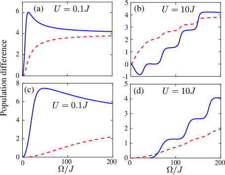
Figure 2: (Color online) Population differences are plotted as a function of $\Omega/J$ for the ground state of the system and $N=8$. The parameters are shown: (a) and (b) $\Delta=20J$; (c) and (d) $\Delta=200J$. The ground state $|g\rangle$ and excited state $|e\rangle$ of atoms are denoted by blue-solid and red-dotted lines, respectively.

In Figs. 2(b) and (d), we plot the population differences versus the coupling strengths $\Omega$ in the regime of strong atomic interactions. We can see that discrete steps of the population difference for atoms in the state $|g\rangle$ are shown when the coupling strength increases. However, the discrete feature is not obvious for the atoms in the state $|e\rangle$. In Fig. 2(b), the atoms, in the two different internal states, distribute in the opposite potential wells for small $\Omega$. When $\Omega$ becomes larger, both component of atoms populate in the left potential well. This result shows that the population difference of atoms in the two internal states depends on the coupling strength and also the detuning between the atoms and field.

To proceed, we investigate the relationship between the total population difference of atoms ($\langle{n_{eL}}+{n_{gL}}-{n_{eR}}-n_{gR}\rangle$) and the coupling strength $\Omega$. In Fig. 3, we plot the total population differences as a function of the coupling strength $\Omega$ for different strengths $U$ of atomic interactions. The external field leads to the population imbalance between two wells in both regimes of weak and strong atomic interactions. For weak atomic interactions, the population difference smoothly increases with $\Omega$. When the atomic interactions become strong, the discrete steps of population differences are shown in Fig. 3. The sharper discrete steps are shown for larger $U$. In this case, a single atom is only allowed to tunnel through the other well for the specific coupling strengths.

III.1 Tunneling condition in the limit of strong atomic interactions

We now discuss the tunneling condition in the limit of strong atomic interactions. Since the tunnel couplings are negligible in this regime, the numbers of atoms in the two wells are conserved. We assume that there are $N/2+n$ and $N/2-n$ atoms in the left and right wells. For convenience, we define the angular momentum operators: $S_{jx}=(g_{j}e^{\dagger}_{j}+e_{j}g^{\dagger}_{j})/2$, $S_{jy}=(g_{j}e^{\dagger}_{j}-e_{j}g^{\dagger}_{j})/2i$ and $S_{jz}=(e^{\dagger}_{j}e_{j}-g^{\dagger}_{j}g_{j})/2$, and $j=L,R$.

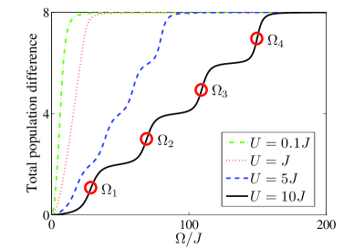
Figure 3: (Color online) Plot of the total population difference versus $\Omega/J$ for the ground state with the different strengths $U$ of atomic interactions. The parameters are used: $N=8$ and $\Delta=20J$. The values of $\Omega_{n}$ in Eq. (6) are marked with the red empty circles.

To diagonalize the Hamiltonian $H_{\rm tot}$, we apply the transformation as

$$S_{Lx} = \cos\theta{S_{Lx}^{\prime}}-\sin\theta{S_{Lz}^{\prime}},$$ (3)

$$S_{Lz} = \cos\theta{S_{Lz}^{\prime}}+\sin\theta{S_{Lx}^{\prime}}.$$ (4)

By setting the term, $\Delta\sin\theta+2\Omega\cos\theta$, to zero, the total Hamiltonian can be diagonalized as

$$H_{\rm tot}^{\prime} = {\Delta}S_{Rz}+\hbar\sqrt{\Delta^{2}+4\Omega^{2}}S_{Lz}^{\prime}+U(N^{2}/2+2n^{2})$$ (5)

$$+\hbar\Delta{N}/2,$$

and its ground-state energy $E^{G}_{n}$ is given by

$$E^{\rm G}_{n} = -\Delta(N/2-n)/2-\sqrt{\Delta^{2}+4\Omega^{2}}(N/2+n)/2$$ (6)

$$+2{U}n^{2}+UN^{2}/2+\Delta{N}/2.$$

The tunneling of atoms occurs when the energies $E^{\rm G}_{n}$ and $E^{\rm G}_{n-1}$ are equal to each other. In this situation, a single atom tunnels through the other well. It is analogous to the resonant tunneling in quantum dots due to the Coulomb blockade Beenakker . By setting $E^{\rm G}_{n}=E^{\rm G}_{n-1}$ in Eq. (6), the tunneling condition for the coupling strength $\Omega_{n}$ can be obtained as

$$\Omega_{n} = \frac{1}{2}\{[4U(2n-1)+\Delta]^{2}-\Delta^{2}\}^{\frac{1}{2}}.$$ (7)

In Fig. 3, the values of $\Omega_{n}$ are marked with the red empty circles. This shows that the tunneling condition in Eq. (7) agrees with the exact numerical solution.

IV Adiabatic transport

We have studied the ground-state properties of the coupled atom-laser system in the previous section. We have shown that the directions of atomic currents and the population difference depend on the coupling strength $\Omega$. Now we study the adiabatic transport of atoms by slowly increasing the coupling strength $\Omega$. According to the adiabatic theorem Messiah , the system can evolve as its instantaneous ground state if the changing rate of the parameter $\Omega$ is sufficiently slow. Therefore, this method can be used for adiabatically transferring the atoms to the other potential well.

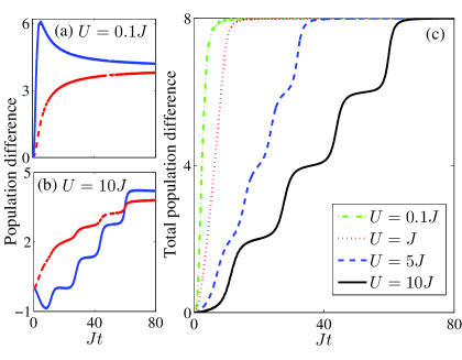
Figure 4: (Color online) The population differences for the two different component condensates are plotted against the time $Jt$ for $U=0.1J$ and $10J$ in (a) and (b). The atoms in ground and excited states are denoted by blue-solid and red-dashed lines, respectively. (c) Plot of the total population difference versus the time $Jt$ for different strengths of atomic interactions. The parameters are used: $N=8$, $\Delta=20J$ and $v=2.5J$.

We consider the coupling strength $\Omega(t)$ as a linear function of time $t$, i.e.,

$$\Omega(t) = v{t},$$ (8)

where $v$ is a positive number. Here the detuning $\Delta$ is kept as a constant during the time evolution. Initially, the system is prepared in its ground state of the Hamiltonian $H_{0}$ in Eq. (1) and setting $\Omega=0$. The coupling strength $\Omega(t)$ in Eq. (8) is adiabatically increased. In Figs. 4(a) and (b), the population differences are plotted versus the time for the atoms in the different internal states. We can see that the two results in Figs. 2 and 4 reach a good agreement. This shows that the tunneling dynamics of atoms can be controlled by using an external field.

In the regime of weak atomic interactions, the two different component condensates smoothly tunnel through the other well in the same direction in Fig. 4(a). In the opposite interaction limit, the discrete steps are shown in Fig. 4(b). Note that the counter-flow is shown in a short time in figure (b). The flows of atomic spin currents become parallel afterward. This shows that the direction of spin flows can be controlled by appropriately adjusting the parameters $\Omega$ and $\Delta$.

Then, we study the time evolution of total population difference of atoms. In Fig. 4(c), we examine the tunneling dynamics for a wide range of interaction parameters. In both regimes, the atoms tunnel to the left potential well when the coupling strength slowly increases with time. The total population differences smoothly increases as a function of time for weak atomic interactions. The discrete steps of the tunneling are shown when the strength of atomic interactions becomes strong. The single-atom tunneling can thus be achieved in the limit of strong atomic interactions.

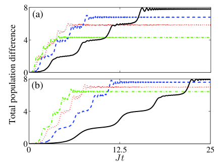
Figure 5: (Color online) The total population differences are plotted versus the time $Jt$ for the different detunings $\Delta=20J$ and $200J$ in (a) and (b), respectively. The different rates of change are denoted: $v=10J$ (black-solid line), $v=20J$ (blue-dashed line), $v=30J$ (red-dotted line) and $v=40J$ (green-dashed-dotted line), respectively. The parameters are used: $N=8$ and $U=10J$.

IV.1 Efficiency of the population difference

Next, we investigate the efficiency of the population transfer by increasing the coupling strength of the external field. In Figs. 5(a) and (b), the population differences are plotted versus the time for the two different detunings $\Delta=20J$ and $200J$. The full population transfer can be achieved if the parameters $v$ are small enough in both cases. When the parameters $v$ become larger, the rates of population transfer increase. However, the smaller population of atoms can be transferred in both cases. It is because they have gone beyond the adiabatic limit. By comparing the figures 5(a) and (b), we find that the larger numbers of atoms can be transported with the same rate $v$ of change for the case using a larger detuning.

IV.2 Effects of the coupling between the laser and the atoms in the neighboring well

Since the separation between the two wells is small Albiez ; Maussang , the lasers may also couple the atoms in the other potential well. Now we examine a very small coupling between the laser and the atoms in the right potential well. The Hamiltonian, describes the coupling between the laser and the atoms in the right potential well, can be written as

$$H^{\rm R}_{1}=\Omega^{\prime}(e^{\dagger}_{R}g_{R}+g^{\dagger}_{R}e_{R}),$$ (9)

where $\Omega^{\prime}$ is the coupling strength between the laser and atoms.

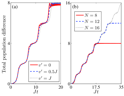
Figure 6: (Color online) Time evolution of the total population difference. The effect of a small coupling between the laser and the atoms in the right potential well is investigated. In (a), the total population differences are plotted versus the time $Jt$ for different rates of changing $v^{\prime}$ and $N=8$. In (b), the total population differences are plotted versus the time $Jt$ for different numbers of atoms and $v^{\prime}=J$. The parameters are used: $U=10J$, $\Delta=20J$ and $v=10J$.

Here we consider that the coupling strength $\Omega^{\prime}$ linearly increases with time as

$$\Omega^{\prime}(t)=v^{\prime}t.$$ (10)

We assume that the parameter $v^{\prime}$ is much smaller than $v$ in Eq. (8).

In Fig. 6(a), the total population differences are plotted versus the time for the different rates of changing $v^{\prime}$. The atoms can be efficiently transferred from the left to right potential well. The results show slightly different tunneling behaviors for small $v^{\prime}$. We then examine the population transfer with small $v^{\prime}$ for larger number of atoms. In Fig. 6(b), we plot the total population difference as a function of time for different numbers of atoms. The discrete steps of tunneling can be clearly shown. This shows that this method works even if there is a very small coupling between the laser and the atoms in the neighboring well.

V Multi-particle entanglement

Having discussed the tunneling dynamics of atoms, we study the generation of spin-squeezed states by adiabatically changing the coupling strength of the field. To indicate the occurrence of spin squeezing, a parameter $\xi^{2}$ can be defined as Wineland

$$\xi^{2} = \frac{N(\Delta{S_{n_{1}}})^{2}}{\langle{S_{n_{2}}}\rangle^{2}+\langle{S_{n_{3}}}\rangle^{2}},$$ (11)

where $n_{i}$ is the $i$-th component of an angular momentum system, and $i=1,2$ and 3. If $\xi$ is less than one, then the system is said to be spin-squeezed Wineland . In addition, the parameter $\xi$ can be used for indicating multi-particle entanglement Sorensen .

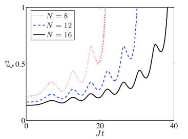
Figure 7: (Color online) The spin-squeezing parameters $\xi^{2}$ are plotted versus the time $Jt$ for different number $N$ of atoms. The parameters are used: $\Delta=200J$, $U=10J$ and $v=10J$.

Let us define the angular momentum operators as: $S_{x}=(e^{\dagger}_{L}e_{R}+g^{\dagger}_{L}g_{R}+e^{\dagger}_{R}e_{L}+g^{\dagger}_{R}g_{L})/2$, $S_{y}=(e^{\dagger}_{L}e_{R}+g^{\dagger}_{L}g_{R}-e^{\dagger}_{R}e_{L}-g^{\dagger}_{R}g_{L})/2i$, and $S_{z}=(e^{\dagger}_{L}e_{R}+g^{\dagger}_{L}g_{L}-e^{\dagger}_{R}e_{R}-g^{\dagger}_{R}g_{R})/2$. The angular momentum operators obey the standard commutation rule. We study the parameter as

$$\xi^{2} = \frac{N(\Delta{S_{z}})^{2}}{\langle{S_{x}}\rangle^{2}}.$$ (12)

Physically speaking, the quantity $(\Delta{S}_{z})^{2}$ is the variance of the total population difference of atoms between the wells, and $\langle{S}_{x}\rangle$ is the sum of the phase coherences between the two wells for the two component condensates.

In Fig. 7, we plot the spin-squeezing parameter $\xi^{2}$ versus the time for different number of atoms. Initially, the parameter $\xi^{2}$ is below one when $\Omega=0$. This means that the initial ground state is a spin-squeezed state. As $\Omega$ in Eq. (7) slowly increases with time, spin squeezing can be dynamically produced. This result indicates that the system is spin-squeezed for a wide range of $\Omega$. Besides, a higher degree of spin squeezing can be produced with a larger number of atoms $N$.

VI Conclusions

In summary, we have studied how the ground state of a two-component condensate in a double well affected by a local external field. We have shown that the flows of spin currents and particle-tunneling dynamics can be controlled by slowly varying the coupling strength of the external field and appropriately adjusting the detuning. This can be used for studying spin and tunneling phenomena and also the potential applications of atomic devices in atomtronics Pepino . In addition, spin-squeezed states can be dynamical generated. It is an important resource for precision measurement Wineland ; Kitagawa ; Sorensen .

Appendix A Derivation of the effective Hamiltonian for coupling between two internal states and the lasers

The two internal states of an atom can be coupled via pumping to the upper state by two lasers as shown in Fig. 1(b). The Hamiltonian, describes the interaction between the two internal states and the lasers, can be written as

$$H = \omega_{rg}|r\rangle\langle{r}|+\omega_{eg}|e\rangle\langle{e}|+\Omega_{g}[\exp{(-i\omega_{g}{t})}|r\rangle\langle{g}|+{\rm H.c.}]$$ (13)

$$+\Omega_{e}[\exp{(-i\omega_{e}{t})}|r\rangle\langle{e}|+{\rm H.c.}],$$

By performing the unitary transformation as,

$$U(t) = \exp\{-i[\omega_{g}|r\rangle\langle{r}|+(\omega_{g}+\omega_{e})|e\rangle\langle{e}|]t\},$$ (14)

the Hamiltonian can be transformed as Barnett

$$H^{\prime} = i\dot{U}^{{\dagger}}U+U^{\dagger}{H}U,$$

$$= \Delta_{r}|r\rangle\langle{r}|+\Delta_{e}|e\rangle\langle{e}|+(\Omega_{g}|r\rangle\langle{g}|+\Omega_{e}|r\rangle\langle{e}|+{\rm H.c.}),$$

where $\Delta_{r}=\omega_{rg}-\omega_{g}$ and $\Delta_{e}=\omega_{eg}-\omega_{g}+\omega_{e}$.

We write the state $|\Psi(t)\rangle$ as,

$$|\Psi(t)\rangle=c_{g}|g\rangle+c_{e}|e\rangle+c_{r}|r\rangle.$$ (17)

From the Schrödinger equation, we can obtain

$$i\dot{c}_{g} = \Omega_{g}c_{r},$$ (18)

$$i\dot{c}_{e} = \Delta_{e}c_{e}+\Omega_{e}c_{r},$$ (19)

$$i\dot{c}_{r} = \Delta_{r}c_{r}+\Omega_{g}c_{g}+\Omega_{e}c_{e}.$$ (20)

We assume that $\Omega_{e}$ and $\Omega_{g}$ are real numbers.

If the detuning $\Delta$ is much greater than the coupling strengths $\Omega_{e},\Omega_{g}$, then the upper state can be adiabatically eliminated. We can obtain

$$c_{r}\approx-\frac{\Omega_{g}}{\Delta_{r}}c_{g}-\frac{\Omega_{e}}{\Delta_{r}}c_{e}.$$ (21)

The effective Hamiltonian can thus be obtained as

$$H_{\rm eff}=-\frac{\Omega^{2}_{g}}{\Delta_{r}}|g\rangle\langle{g}|+\Big{(}\Delta_{e}-\frac{\Omega^{2}_{e}}{\Delta_{r}}\Big{)}|e\rangle\langle{e}|+\Omega(|g\rangle{\langle}e|+{\rm H.c.}),$$ (22)

where $\Omega=-\Omega_{e}\Omega_{g}/{\Delta_{r}}$ is the effective coupling strength between the two internal states $|g\rangle$ and $|e\rangle$. We assume that $\Omega_{g}$ and $\Omega_{e}$ are approximately equal and let $\Delta_{e}=\Delta$ in Eq. (2).

References

- (1) A. Fert, Rev. Mod. Phys. 80, 1517 (2008).
- (2) M. A. Nielsen and I. L. Chuang, Quantum Computation and Quantum Information (Cambridge University Press, Cambridge, 2000).
- (3) M. Albiez, et al., Phys. Rev. Lett. 95, 010402 (2005).
- (4) S. Fölling, et al., Nature 448, 1029 (2007).
- (5) W. S. Bakr et al., Nature 462 74 (2009)
- (6) C. Weitenberg et al., Nature 471, 319 (2011).
- (7) J. Volz et al., Nature 475, 210 (2011).
- (8) H. T. Ng, C. K. Law, and P. T. Leung, Phys. Rev. A 68, 013604 (2003).
- (9) M. Holthaus, Phys. Rev. A, 64, 011601(R) (2001); C. Weiss and T. Jinasundera, Phys. Rev. A 72, 053626 (2005); T. Jinasundera, C. Weiss, M. Holthaus, Chem. Phys. 322, 118 (2006).
- (10) L. Morales-Molina and J. Gong, Phys. Rev. A 78, 041403(R) (2008).
- (11) L. Forster, et al., Phys. Rev. Lett. 103, 233001 (2009); Q. Beaufils et al., ibid. 106, 213002 (2011).
- (12) D. R. Dounas-Frazer, A. M. Hermundstad and L. D. Carr, Phys. Rev. Lett. 99 200402 (2007); P. Cheinet et al., ibid. 101, 090404 (2008).
- (13) C. E. Creffield, Phys. Rev. Lett. 99, 110501 (2007); O. Romero-Isart and J. J. García-Ripoll, Phys. Rev. A 76, 052304 (2007); Y. Qian, Ming Gong and C. Zhang, ibid. 84, 013608 (2011).
- (14) D. M. Harber et al., Phys. Rev. A 66, 053616 (2002).
- (15) A. B. Kuklov and B. V. Svistunov, Phys. Rev. Lett. 90, 100401 (2003).
- (16) M. Kitagawa and M. Ueda, Phys. Rev. A 47, 5138 (1993).
- (17) D. J. Wineland, J. J. Bollinger, W. M. Itano and D. J. Heinzen, Phys. Rev. A 50, 67 (1994).
- (18) A. Sorensen, L.-M. Duan, I. Cirac, P. Zoller, Nature 409, 63 (2001).
- (19) J. Estève et al., Nature 455, 1216 (2008); M. F. Riedel et al., ibid. 464, 1170 (2010).
- (20) M. R. Matthews et al., Phys. Rev. Lett. 81, 243 (1998).
- (21) G. J. Milburn, J. Corney, E. M. Wright and D. F. Walls, Phys. Rev. A 55, 4318 (1997).
- (22) K. Maussang et al., arXiv:1005.1922..
- (23) D. A. Steck, Rubidium 87 D line data, http://steck.us/alkalidata/ (2010)
- (24) S. M. Barnett and P. M. Radmore, Methods in Theoretical Quantum Optics (Oxford University Press, Oxford, 2002).
- (25) C. W. J. Beenakker, Phys. Rev. B 44, 1646 (1991).
- (26) A. Messiah, Quantum Mechanics (Dover, New York, 1999).
- (27) R. A. Pepino, J. Cooper, D. Z. Anderson and M. J. Holland, Phys. Rev. Lett. 103, 140405 (2009).