Joint $k$-step analysis of Orthogonal Matching Pursuit and Orthogonal Least Squares

Abstract

Tropp’s analysis of Orthogonal Matching Pursuit (OMP) using the Exact Recovery Condition (ERC) [1] is extended to a first exact recovery analysis of Orthogonal Least Squares (OLS). We show that when the ERC is met, OLS is guaranteed to exactly recover the unknown support in at most $k$ iterations. Moreover, we provide a closer look at the analysis of both OMP and OLS when the ERC is not fulfilled. The existence of dictionaries for which some subsets are never recovered by OMP is proved. This phenomenon also appears with basis pursuit where support recovery depends on the sign patterns, but it does not occur for OLS. Finally, numerical experiments show that none of the considered algorithms is uniformly better than the other but for correlated dictionaries, guaranteed exact recovery may be obtained after fewer iterations for OLS than for OMP.

I Introduction

Classical greedy subset selection algorithms include, by increasing order of complexity: Matching Pursuit (MP) [2], Orthogonal Matching Pursuit (OMP) [3] and Orthogonal Least Squares (OLS) [4, 5]. OLS is indeed relatively expensive in comparison with OMP since OMP performs one linear inversion per iteration whereas OLS performs as many linear inversions as there are non-active atoms. We refer the reader to the technical report [6] for a comprehensive review on the difference between OMP and OLS.

OLS is referred to using many other names in the literature. It is known as forward selection in statistical regression [7] and as the greedy algorithm [5], Order Recursive Matching Pursuit (ORMP) [8] and Optimized Orthogonal Matching Pursuit (OOMP) [9] in the signal processing literature, all these algorithms being actually the same. It is worth noticing that the above-mentioned algorithms were introduced by following either an optimization [4, 7] or an orthogonal projection methodology [5], or both [8, 9]. In the optimization viewpoint, the atom yielding the largest decrease of the approximation error is selected. This leads to a greedy sub-optimal algorithm dedicated to the minimization of the approximation error. In the orthogonal projection viewpoint, the atom selection rule is defined as an extension of the OMP rule: the data vector and the dictionary atoms are being projected onto the subspace that is orthogonal to the span of the active atoms, and the normalized projected atom having the largest inner product with the data residual is selected. As the number of active atoms increases by one at any iteration, the projections are done on a subspace whose dimension is decreasing.

I-A Main objective of the paper

Our primary goal is to address the OLS exact recovery analysis from noise-free data and to investigate the connection between the OMP and OLS exact recovery conditions. In the literature, much attention was paid to the exact recovery analysis of sparse algorithms that are faster than OLS, e.g., thresholding algorithms and simpler greedy algorithms like OMP [10]. But to the best of our knowledge, no exact recovery result is available for OLS. In their recent paper [11], Davies and Eldar mention this issue and state that the relation between OMP and OLS remains unclear.

I-B Existing results for OMP

Our starting point is the existing $k$-step analysis of OMP whose structure is somewhat close to OLS. The notion of $k$-step solution property was defined in [12]: “any vector with at most $k$ nonzeros can be recovered from the related noise-free observation in at most $k$ iterations.” The $k$-step property will also be referred to as the “exact support recovery” in the following. Exact recovery studies of OMP rely on alternate methodologies.

Tropp’s Exact Recovery Condition (ERC) [1] is a necessary and sufficient condition of exact support recovery in a worst case analysis. On the one hand, if a subset of $k$ atoms satisfies the ERC, then it can be recovered from any linear combination of the $k$ atoms in at most $k$ steps. On the other hand, when the ERC is not satisfied, one can generate a counterexample (i.e., a specific combination of the $k$ atoms) for which OMP fails, i.e., OMP selects a wrong atom during its first $k$ iterations. Specifically, the atom selected in the first iteration is a wrong one.

Davenport and Wakin [13] used another analysis to show that OMP yields exact support recovery under certain Restricted Isometry Property (RIP) assumptions, and several improvements of their condition were proposed more recently [14, 15]. Actually, the ERC necessarily holds when the latter conditions are fulfilled since the ERC is a sufficient and worst case necessary condition of exact recovery.

I-C Generalization of Tropp’s condition

We propose to extend Tropp’s condition to OLS. We remark that the very first iteration of OLS is identical to that of OMP: the first selected atom is the one whose inner product with the input vector is maximal. Therefore, when the ERC does not hold, the counterexample for which the first iteration of OMP fails also yields a failure of the first iteration of OLS. Hence one cannot expect to derive an exact recovery condition for OLS that would be weaker than the ERC at the first iteration. We show that the ERC indeed ensures the success of OLS.

We further address the case where the ERC does not hold, i.e., the first iteration of OMP/OLS is not guaranteed to always succeed but nevertheless succeeds for a given vector. In practice, even for non random dictionaries, this phenomenon is likely to occur since the ERC is a worst case necessary condition. The purpose of a large part of the paper is specifically to analyze what is going on in the remaining iterations for these vectors. With $\ell_{1}$ minimization, the situation is clearer because support recovery depends on the sign patterns [16, Theorem 2] and one can predict whether a specific vector will be recovered independently of the support amplitudes. For greedy algorithms, things are more tricky and it is one of the purpose of the paper to analyze this. We introduce weaker conditions than the ERC which guarantee that an exact support recovery will occur in the subsequent iterations. These extended recovery conditions coincide with the ERC at the first iteration but differ from it afterwards.

Our main results state that:

• The ERC is a sufficient condition of exact recovery for OLS in at most $k$ steps (Theorem 2).

• When the early iterations of OMP/OLS have all succeeded, we derive two sufficient conditions, named ERC-OMP and ERC-OLS, for the recovery of the remaining true atoms (Theorem 3). This result is a ($k-q$)-step property, where $q$ stands for the number of iterations which have been already performed.

• Moreover, we show that our conditions are, in some sense, necessary (Theorems 4 and 5).

The criteria we provide might not necessarily be directly useful for practitioners working in the field. In fact, just as many other theoretical success guarantees, they are rather “motivational”: by proving that the considered algorithms are guaranteed to perform well in a restricted regime, they strengthen our confidence that the heuristics behind the algorithms are reasonably grounded. Practitioners know that the algorithms indeed work much beyond the considered restricted regime, but proving this fact would typically require probabilistic arguments, based on models of random dictionary or random input signals [17, 18]. Despite their potential interest, the theoretical results that can be foreseen in this spirit would be highly dependent on the adequacy of such models to the actual distribution of data from the real world.

I-D Organization of the paper

In Section II, we recall the principle of OMP and OLS and their interpretation in terms of orthogonal projections. Then, we properly define the notions of successful support recovery and support recovery failure. Section III is dedicated to the analysis of OMP and OLS at any iteration where the most technical developments and proofs are omitted for readability reasons. These important elements can be found in the appendix section A. In Section IV, we show using Monte Carlo simulations that there is no systematic implication between the ERC-OMP and ERC-OLS conditions but we exhibit some elements of discrimination in favor of OLS.

II Notations and prerequisites

The following notations will be used in this paper. $\langle\,.\,,\,.\,\rangle$ refers to the inner product between vectors, and $\|\,.\,\|$ and $\|\,.\,\|_{1}$ stand for the Euclidean norm and the $\ell_{1}$ norm, respectively. $.^{\dagger}$ denotes the pseudo-inverse of a matrix. For a full rank and undercomplete matrix, we have ${\mathb{X}}^{\dagger}=({\mathb{X}}^{t}{\mathb{X}})^{-1}{\mathb{X}}^{t}$ where $.^{t}$ stands for the matrix transposition. When $\mathb{X}$ is overcomplete, ${\mathrm{spark}}({\mathb{X}})$ denotes the minimum number of columns from $\mathb{X}$ that are linearly dependent [19]. The letter $\mathcal{Q}$ denotes some subset of the column indices, and ${\mathb{X}}_{{\mathcal{Q}}}$ is the submatrix of $\mathb{X}$ gathering the columns indexed by $\mathcal{Q}$. Finally, ${\mathb{P}}_{\mathcal{Q}}={\mathb{X}}_{\mathcal{Q}}{\mathb{X}}_{\mathcal{Q}}^{\dagger}$ and ${\mathb{P}}_{\mathcal{Q}}^{\perp}={\mathb{I}}-{\mathb{P}}_{\mathcal{Q}}$ denote the orthogonal projection operators on ${\mathrm{span}}({\mathb{X}}_{\mathcal{Q}})$ and ${\mathrm{span}}({\mathb{X}}_{\mathcal{Q}})^{\perp}$, where ${\mathrm{span}}({\mathb{X}})$ stands for the column span of $\mathb{X}$, ${\mathrm{span}}({\mathb{X}})^{\perp}$ is the orthogonal complement of ${\mathrm{span}}({\mathb{X}})$ and $\mathb{I}$ is the identity matrix whose dimension is equal to the number of rows in $\mathb{X}$.

II-A Subset selection

Let ${\mathb{A}}=[{\mathb{a}}_{1},\ldots,{\mathb{a}}_{n}]$ denote the dictionary gathering normalized atoms ${\mathb{a}}_{i}\in{\mathbbm{R}}^{m}$. $\mathb{A}$ is a matrix of size $m\times n$. Assuming that the atoms are normalized is actually not necessary for OLS as the behavior of OLS is unchanged whether the atoms are normalized or not [6]. On the contrary, OMP is highly sensitive to the normalization of atoms since its selection rule involves the inner products between the current residual and the non-selected atoms.

We consider a subset ${\mathcal{Q}}^{\star}$ of $\{1,\ldots,n\}$ of cardinality $k\triangleq{\mathrm{Card}}\left[{\mathcal{Q}}^{\star}\right]<\min(m,n)$ and study the behavior of OMP and OLS for all inputs ${\mathb{y}}\in{\mathrm{span}}({\mathb{A}}_{{\mathcal{Q}}^{\star}})$, i.e., for any combination ${\mathb{y}}={\mathb{A}}_{{\mathcal{Q}}^{\star}}{\mathb{t}}$ where the submatrix ${\mathb{A}}_{{\mathcal{Q}}^{\star}}$ is of size $m\times k$ and the weight vector ${\mathb{t}}\in{\mathbbm{R}}^{k}$. The $k$ atoms $\{{\mathb{a}}_{i},\,i\in{\mathcal{Q}}^{\star}\}$ indexed by ${\mathcal{Q}}^{\star}$ will be referred to as the “true” atoms while for the remaining (“wrong”) atoms $\{{\mathb{a}}_{j},\,j\notin{\mathcal{Q}}^{\star}\}$, we will use the subscript notation $j$. The forward greedy algorithms considered in this paper start from the empty support and select a new atom per iteration. At intermediate iterations $q\in\{0,\ldots,k-1\}$, we denote by $\mathcal{Q}$ the current support (with ${\mathrm{Card}}\left[{\mathcal{Q}}\right]=q$).

Throughout the paper, we make the general assumption that ${\mathb{A}}_{{\mathcal{Q}}^{\star}}$ is full rank. Note that the representation ${\mathb{y}}={\mathb{A}}_{{\mathcal{Q}}^{\star}}{\mathb{t}}$ is not guaranteed to be unique under this assumption: there may be another $k$-term representation ${\mathb{y}}={\mathb{A}}_{{\mathcal{Q}}^{\prime}}{\mathb{t}}^{\prime}$ where ${\mathb{A}}_{{\mathcal{Q}}^{\prime}}$ includes some wrong atoms ${\mathb{a}}_{j}$. The stronger assumption ${\mathrm{spark}}({\mathb{A}})>2k$ is a necessary and sufficient condition for uniqueness of any $k$-term representation [19]. Therefore, when ${\mathrm{spark}}({\mathb{A}})>2k$, the selection of a wrong atom by a greedy algorithm disables a $k$-term representation of $\mathb{y}$ in $k$ steps [1]. We make the weak assumption that ${\mathb{A}}_{{\mathcal{Q}}^{\star}}$ is full rank because it is sufficient to elaborate our exact recovery conditions under which no wrong atom is selected in the first $k$ iterations.

II-B OMP and OLS algorithms

The common feature between OMP and OLS is that they both perform an orthogonal projection whenever the support $\mathcal{Q}$ is updated: the data approximation reads ${\mathb{P}}_{\mathcal{Q}}{\mathb{y}}$ and the residual error is defined by

$${\mathb{r}}_{\mathcal{Q}}\triangleq{\mathb{y}}-{\mathb{P}}_{\mathcal{Q}}{\mathb{y}}={\mathb{P}}_{{\mathcal{Q}}}^{\perp}{\mathb{y}}.$$

Let us now recall how the selection rule of OLS differs from that of OMP.

At each iteration of OLS, the atom ${\mathb{a}}_{\ell}$ yielding the minimum least-square error $\|{\mathb{r}}_{{\mathcal{Q}}\cup\{\ell\}}\|^{2}$ is selected:

$$\ell^{\textrm{OLS}}\in\mathop{\mathrm{arg\,min}}_{i\notin{\mathcal{Q}}}\|{\mathb{r}}_{{\mathcal{Q}}\cup\{i\}}\|^{2}$$

and $n-{\mathrm{Card}}\left[{\mathcal{Q}}\right]$ least-square problems are being solved to compute $\|{\mathb{r}}_{{\mathcal{Q}}\cup\{i\}}\|^{2}$ for all $i\notin{\mathcal{Q}}$ () [4]. On the contrary, OMP adopts the simpler rule

$$\ell^{\textrm{OMP}}\in\mathop{\mathrm{arg\,max}}_{i\notin{\mathcal{Q}}}|\langle{\mathb{r}}_{\mathcal{Q}},{\mathb{a}}_{i}\rangle|$$

to select the new atom ${\mathb{a}}_{\ell}$ and then solves only one least-square problem to update ${\mathb{r}}_{{\mathcal{Q}}\cup\{\ell\}}$ [6]. Depending on the application, the OMP and OLS stopping rules can involve a maximum number of atoms and/or a residual threshold. Note that when the data are noise-free (they read as ${\mathb{y}}={\mathb{A}}_{{\mathcal{Q}}^{\star}}{\mathb{t}}$) and no wrong atom is selected, the squared error $\|{\mathb{r}}_{{\mathcal{Q}}}\|^{2}$ is equal to 0 after at most $k$ iterations. Therefore, we will consider no more than $k$ iterations in the following.

II-C Geometric interpretation

A geometric interpretation in terms of orthogonal projections will be useful for deriving recovery conditions. It is essentially inspired by the technical report of Blumensath and Davies [6] and by Davenport and Wakin’s analysis of OMP under the RIP assumption [13].

We introduce the notation $\tilde{{\mathb{a}}}_{i}={\mathb{P}}_{{\mathcal{Q}}}^{\perp}{\mathb{a}}_{i}$ for the projected atoms onto ${\mathrm{span}}({\mathb{A}}_{\mathcal{Q}})^{\perp}$ where for simplicity, the dependence upon $\mathcal{Q}$ is omitted. When there is a risk of confusion, we will use $\tilde{{\mathb{a}}}_{i}^{{\mathcal{Q}}}$ instead of $\tilde{{\mathb{a}}}_{i}$. Notice that $\tilde{{\mathb{a}}}_{i}={\mathbf{0}}$ if and only if ${\mathb{a}}_{i}\in{\mathrm{span}}({\mathb{A}}_{\mathcal{Q}})$. In particular, $\tilde{{\mathb{a}}}_{i}={\mathbf{0}}$ for $i\in{\mathcal{Q}}$. Finally, we define the normalized vectors

$$\tilde{{\mathb{b}}}_{i}=\left\{\begin{array}[]{cl}{\tilde{{\mathb{a}}}_{i}/\|\tilde{{\mathb{a}}}_{i}\|}&\textrm{if}~{}\tilde{{\mathb{a}}}_{i}\neq{\mathbf{0}},\\ {\mathbf{0}}&\textrm{otherwise}.\end{array}\right.$$

Again, we will use $\tilde{{\mathb{b}}}_{i}^{{\mathcal{Q}}}$ when there is a risk of confusion.

We now emphasize that the projected atoms $\tilde{{\mathb{a}}}_{i}$ (or $\tilde{{\mathb{b}}}_{i}$) play a central role in the analysis of both OMP and OLS. Because the residual ${\mathb{r}}_{\mathcal{Q}}={\mathb{P}}_{{\mathcal{Q}}}^{\perp}{\mathb{y}}$ lays in ${\mathrm{span}}({\mathb{A}}_{\mathcal{Q}})^{\perp}$, $\langle{\mathb{r}}_{\mathcal{Q}},{\mathb{a}}_{i}\rangle=\langle{\mathb{r}}_{\mathcal{Q}},\tilde{{\mathb{a}}}_{i}\rangle$ and the OMP selection rule rereads:

$$\ell^{\textrm{OMP}}\in\mathop{\mathrm{arg\,max}}_{i\notin{\mathcal{Q}}}|\langle{\mathb{r}}_{\mathcal{Q}},\tilde{{\mathb{a}}}_{i}\rangle|$$ (1)

whereas for OLS, minimizing $\|{\mathb{r}}_{{\mathcal{Q}}\cup\{i\}}\|^{2}$ with respect to $i\notin{\mathcal{Q}}$ is equivalent to maximizing $\|{\mathb{r}}_{{\mathcal{Q}}}\|^{2}-\|{\mathb{r}}_{{\mathcal{Q}}\cup\{i\}}\|^{2}=\langle{\mathb{r}}_{\mathcal{Q}},\tilde{{\mathb{b}}}_{i}\rangle^{2}$ (see e.g., [9] for a complete calculation):

$$\ell^{\textrm{OLS}}\in\mathop{\mathrm{arg\,max}}_{i\notin{\mathcal{Q}}}|\langle{\mathb{r}}_{\mathcal{Q}},\tilde{{\mathb{b}}}_{i}\rangle|.$$ (2)

We notice that (1) and (2) only rely on the vectors ${\mathb{r}}_{\mathcal{Q}}$ and $\tilde{{\mathb{a}}}_{i}$ belonging to the subspace ${\mathrm{span}}({\mathb{A}}_{\mathcal{Q}})^{\perp}$. OMP maximizes the inner product $|\langle{\mathb{r}}_{\mathcal{Q}},\tilde{{\mathb{a}}}_{i}\rangle|$ whereas OLS minimizes the angle between ${\mathb{r}}_{\mathcal{Q}}$ and $\tilde{{\mathb{a}}}_{i}$ (this difference was already stressed and graphically illustrated in [6]). When the dictionary is close to orthogonal, e.g., for dictionaries satisfying the RIP assumption, this does not make a strong difference since $\|\tilde{{\mathb{a}}}_{i}\|$ is close to 1 for all atoms [13]. But in the general case, $\|\tilde{{\mathb{a}}}_{i}\|$ may have wider variations between 0 and 1 leading to substantial differences between the behavior of OMP and OLS.

II-D Definition of successful recovery and failure

Throughout the paper, we will use the common acronym Oxx in statements that apply to both OMP and OLS. Moreover, we define the unifying notation:

$$\tilde{{\mathb{c}}}_{i}\triangleq\left\{\begin{array}[]{ll}\tilde{{\mathb{a}}}_{i}&\textrm{for OMP},\\ \tilde{{\mathb{b}}}_{i}&\textrm{for OLS}.\end{array}\right.$$

We first stress that in special cases where the Oxx selection rule yields multiple solutions including a wrong atom, i.e., when

$$\max_{i\in{\mathcal{Q}}^{\star}\backslash{\mathcal{Q}}}|\langle{\mathb{r}}_{\mathcal{Q}},\tilde{{\mathb{c}}}_{i}\rangle| =\max_{j\notin{\mathcal{Q}}^{\star}}|\langle{\mathb{r}}_{\mathcal{Q}},\tilde{{\mathb{c}}}_{j}\rangle|,$$ (3)

we consider that Oxx automatically makes the wrong decision. Tropp used this convention for OMP and showed that when the upper bound on his ERC condition (see Section III-A) is reached, the limit situation (3) occurs, hence a wrong atom is selected at the first iteration [1]. Let us now properly define the $k$-step property for successful support recovery.

Definition 1

Oxx with ${\mathb{y}}\in{\mathrm{span}}({\mathb{A}}_{{\mathcal{Q}}^{\star}})$ as input succeeds if and only if no wrong atom is selected and the residual ${\mathb{r}}_{\mathcal{Q}}$ is equal to $\mathbf{0}$ after at most $k$ iterations.

When a successful recovery occurs, the subset $\mathcal{Q}$ yielded by Oxx satisfies ${\mathcal{Q}}_{\mathb{y}}\subseteq{\mathcal{Q}}\subseteq{\mathcal{Q}}^{\star}$ where ${\mathcal{Q}}_{\mathb{y}}$ is the subset indexed by the nonzero weights $t_{i}$’s in the decomposition ${\mathb{y}}={\mathb{A}}_{{\mathcal{Q}}^{\star}}{\mathb{t}}$. When all $t_{i}$’s are nonzero, ${\mathcal{Q}}_{\mathb{y}}$ identifies with ${\mathcal{Q}}^{\star}$ and a successful recovery cannot occur in less than $k$ iterations.

The word “failure” refers to the exact contrary of successful recovery.

Definition 2

Oxx with ${\mathb{y}}\in{\mathrm{span}}({\mathb{A}}_{{\mathcal{Q}}^{\star}})$ as input fails when at least one wrong atom is selected during the first $k$ iterations. In particular, Oxx fails when (3) occurs with ${\mathb{r}}_{\mathcal{Q}}\neq{\mathbf{0}}$.

The notion of successful recovery may be defined in a weaker sense: Plumbley [16, Corollary 4] pointed out that there exist problems for which the ERC fails but nevertheless, a “delayed recovery” occurs after more than $k$ steps, in that a larger support including ${\mathcal{Q}}^{\star}$ is found, but all atoms which do not belong to ${\mathcal{Q}}^{\star}$ are weighted by 0 in the solution vector. Recently, a delayed recovery analysis of OMP using RIP assumptions was proposed in [20], and then extended to the weak OMP algorithm [21]. In the present paper, no more than $k$ steps are performed, thus delayed recovery is considered as a recovery failure.

III Overview of our recovery analysis of OMP and OLS

In this section, we present our main concepts and results regarding the sparse recovery guarantees with OLS, their connection with the existing OMP results and the new results regarding OMP. For clarity reasons, we place the technical analysis including most of the proofs in the main appendix section A. Let us first recall Tropp’s ERC condition for OMP which is our starting point.

III-A Tropp’s ERC condition for OMP

Theorem 1

[ERC is a sufficient recovery condition for OMP and a necessary condition at the first iteration [1, Theorems 3.1 and 3.10]] If ${\mathb{A}}_{{\mathcal{Q}}^{\star}}$ is full rank and

$$\max_{j\notin{\mathcal{Q}}^{\star}}\{F_{{\mathcal{Q}}^{\star}}({\mathb{a}}_{j})\triangleq\bigl{\|}{\mathb{A}}_{{\mathcal{Q}}^{\star}}^{\dagger}{\mathb{a}}_{j}\bigr{\|}_{1}\}<1, {\mathb{A}},{\mathcal{Q}}^{\star}$$ ERC()

then OMP succeeds for any input ${\mathb{y}}\in{\mathrm{span}}({\mathb{A}}_{{\mathcal{Q}}^{\star}})$. Furthermore, when ERC(${\mathb{A}},{\mathcal{Q}}^{\star}$) does not hold, there exists ${\mathb{y}}\in{\mathrm{span}}({\mathb{A}}_{{\mathcal{Q}}^{\star}})$ for which some wrong atom is selected at the first iteration of OMP. When ${\mathrm{spark}}({\mathb{A}})>2k$, this implies that OMP cannot recover the (unique) $k$-term representation of $\mathb{y}$.

Note that ERC(${\mathb{A}},{\mathcal{Q}}^{\star}$) involves the dictionary atoms but not their weights as it results from a worst case analysis: if ERC(${\mathb{A}},{\mathcal{Q}}^{\star}$) holds, then a successful recovery occurs with ${\mathb{y}}={\mathb{A}}_{{\mathcal{Q}}^{\star}}{\mathb{t}}$ whatever ${\mathb{t}}\in{\mathbbm{R}}^{k}$.

III-B Main theorem

A theorem similar to Theorem 1 applies to OLS.

Theorem 2

[ERC is a sufficient recovery condition for OLS and a necessary condition at the first iteration] If ${\mathb{A}}_{{\mathcal{Q}}^{\star}}$ is full rank and ERC(${\mathb{A}},{\mathcal{Q}}^{\star}$) holds, then OLS succeeds for any input ${\mathb{y}}\in{\mathrm{span}}({\mathb{A}}_{{\mathcal{Q}}^{\star}})$. Furthermore, when ERC(${\mathb{A}},{\mathcal{Q}}^{\star}$) does not hold, there exists ${\mathb{y}}\in{\mathrm{span}}({\mathb{A}}_{{\mathcal{Q}}^{\star}})$ for which some wrong atom is selected at the first iteration of OLS. When ${\mathrm{spark}}({\mathb{A}})>2k$, this implies that OLS cannot recover the (unique) $k$-term representation of $\mathb{y}$.

The necessary condition result is obvious since the very first iteration of OLS coincides with that of OMP and the ERC is a worst case necessary condition for OMP. The core of our contribution is the sufficient condition result for OLS. We now introduce the main concepts on which our analysis relies. They also lead to a more precise analysis of OMP from the second iteration.

III-C Main concepts

Let us keep in mind that the ERC is a worst case necessary condition at the first iteration. But what happens when the ERC is not met but nevertheless, the first $q$ iterations of Oxx select $q$ true atoms ($q<k$)? Can we characterize the exact recovery conditions at the $(q+1)$-th iteration? We will answer to these questions and provide:

1. an extension of the ERC condition to the $q$-th iteration of OMP;

2. a new necessary and sufficient condition dedicated to the $q$-th iteration of OLS.

This will allow us to prove Theorem 2 as a special case of the latter condition when $q=0$.

In the following two paragraphs, we introduce useful notations for a single wrong atom ${\mathb{a}}_{j}$ and then define our new exact recovery conditions by considering all wrong atoms together. $\mathcal{Q}$ plays the role of the subset found by Oxx after the first $q$ iterations.

III-C1 Notations related to a single wrong atom

For ${\mathcal{Q}}\subsetneq{\mathcal{Q}}^{\star}$ and $j\notin{\mathcal{Q}}^{\star}$, we define:

$$F_{{\mathcal{Q}}^{\star},{\mathcal{Q}}}^{\mathrm{OMP}}({\mathb{a}}_{j}) \triangleq\sum_{i\in{\mathcal{Q}}^{\star}\backslash{\mathcal{Q}}}\,\bigl{|}\bigl{(}{\mathb{A}}_{{\mathcal{Q}}^{\star}}^{\dagger}{\mathb{a}}_{j}\bigr{)}(i)\bigr{|}$$ (4)

$$F_{{\mathcal{Q}}^{\star},{\mathcal{Q}}}^{\mathrm{OLS}}({\mathb{a}}_{j}) \triangleq\sum_{i\in{\mathcal{Q}}^{\star}\backslash{\mathcal{Q}}}\frac{\|\tilde{{\mathb{a}}}_{i}\|}{\|\tilde{{\mathb{a}}}_{j}\|}\,\bigl{|}\bigl{(}{\mathb{A}}_{{\mathcal{Q}}^{\star}}^{\dagger}{\mathb{a}}_{j}\bigr{)}(i)\bigr{|}$$ (5)

when $\tilde{{\mathb{a}}}_{j}\neq{\mathbf{0}}$ and $F_{{\mathcal{Q}}^{\star},{\mathcal{Q}}}^{\mathrm{Oxx}}({\mathb{a}}_{j})=0$ when $\tilde{{\mathb{a}}}_{j}={\mathbf{0}}$ (we recall that $\tilde{{\mathb{a}}}_{i}={\mathb{P}}_{{\mathcal{Q}}}^{\perp}{\mathb{a}}_{i}$ and $\tilde{{\mathb{a}}}_{j}={\mathb{P}}_{{\mathcal{Q}}}^{\perp}{\mathb{a}}_{j}$ depend on $\mathcal{Q}$). Up to some manipulations on orthogonal projections, (4) and (5) can be rewritten as follows.

Lemma 1

Assume that ${\mathb{A}}_{{\mathcal{Q}}^{\star}}$ is full rank. For ${\mathcal{Q}}\subsetneq{\mathcal{Q}}^{\star}$ and $j\notin{\mathcal{Q}}^{\star}$, $F_{{\mathcal{Q}}^{\star},{\mathcal{Q}}}^{\mathrm{OMP}}({\mathb{a}}_{j})$ and $F_{{\mathcal{Q}}^{\star},{\mathcal{Q}}}^{\mathrm{OLS}}({\mathb{a}}_{j})$ also read

$$F_{{\mathcal{Q}}^{\star},{\mathcal{Q}}}^{\mathrm{OMP}}({\mathb{a}}_{j}) =\|\tilde{{\mathb{A}}}_{{\mathcal{Q}}^{\star}\backslash{\mathcal{Q}}}^{\dagger}\tilde{{\mathb{a}}}_{j}\|_{1}$$ (6)

$$F_{{\mathcal{Q}}^{\star},{\mathcal{Q}}}^{\mathrm{OLS}}({\mathb{a}}_{j}) =\|\tilde{{\mathb{B}}}_{{\mathcal{Q}}^{\star}\backslash{\mathcal{Q}}}^{\dagger}\tilde{{\mathb{b}}}_{j}\|_{1}$$ (7)

where the matrices $\tilde{{\mathb{A}}}_{{\mathcal{Q}}^{\star}\backslash{\mathcal{Q}}}=\{\tilde{{\mathb{a}}}_{i},\,i\in{\mathcal{Q}}^{\star}\backslash{\mathcal{Q}}\}$ and $\tilde{{\mathb{B}}}_{{\mathcal{Q}}^{\star}\backslash{\mathcal{Q}}}=\{\tilde{{\mathb{b}}}_{i},\,i\in{\mathcal{Q}}^{\star}\backslash{\mathcal{Q}}\}$ of size $m\times(k-q)$ are full rank.

Lemma 1 is proved in Appendix B.

III-C2 ERC-Oxx conditions for the whole dictionary

We define four binary conditions by considering all the wrong atoms together:

$$\max_{j\notin{\mathcal{Q}}^{\star}} \,F_{{\mathcal{Q}}^{\star},{\mathcal{Q}}}^{\mathrm{OMP}}({\mathb{a}}_{j})<1 {\mathb{A}},{\mathcal{Q}}^{\star},{\mathcal{Q}}$$ ERC-OMP()

$$\max_{j\notin{\mathcal{Q}}^{\star}} \,F_{{\mathcal{Q}}^{\star},{\mathcal{Q}}}^{\mathrm{OLS}}({\mathb{a}}_{j})<1 {\mathb{A}},{\mathcal{Q}}^{\star},{\mathcal{Q}}$$ ERC-OLS()

$$\max_{\begin{subarray}{c}{\mathcal{Q}}\subsetneq{\mathcal{Q}}^{\star}\\ {\mathrm{Card}}\left[{\mathcal{Q}}\right]=q\end{subarray}} \max_{j\notin{\mathcal{Q}}^{\star}}F_{{\mathcal{Q}}^{\star},{\mathcal{Q}}}^{\mathrm{OMP}}({\mathb{a}}_{j})<1 {\mathb{A}},{\mathcal{Q}}^{\star},q$$ ERC-OMP()

$$\max_{\begin{subarray}{c}{\mathcal{Q}}\subsetneq{\mathcal{Q}}^{\star}\\ {\mathrm{Card}}\left[{\mathcal{Q}}\right]=q\end{subarray}} \max_{j\notin{\mathcal{Q}}^{\star}}F_{{\mathcal{Q}}^{\star},{\mathcal{Q}}}^{\mathrm{OLS}}({\mathb{a}}_{j})<1 {\mathb{A}},{\mathcal{Q}}^{\star},q$$ ERC-OLS()

We will use the common notations $F_{{\mathcal{Q}}^{\star},{\mathcal{Q}}}^{\mathrm{Oxx}}({\mathb{a}}_{j})$, ERC-Oxx(${\mathb{A}},{\mathcal{Q}}^{\star},{\mathcal{Q}}$) and ERC-Oxx(${\mathb{A}},{\mathcal{Q}}^{\star},q$) for statements that are common to both OMP and OLS.

Remark 1

$F_{{\mathcal{Q}}^{\star},\emptyset}^{\mathrm{OMP}}({\mathb{a}}_{j})$ and $F_{{\mathcal{Q}}^{\star},\emptyset}^{\mathrm{OLS}}({\mathb{a}}_{j})$ both reread $F_{{\mathcal{Q}}^{\star}}({\mathb{a}}_{j})=\bigl{\|}{\mathb{A}}_{{\mathcal{Q}}^{\star}}^{\dagger}{\mathb{a}}_{j}\bigr{\|}_{1}$ since $\tilde{{\mathb{a}}}_{i}^{\emptyset}$ reduces to ${\mathb{a}}_{i}$ which is of unit norm. Thus, ERC-Oxx(${\mathb{A}},{\mathcal{Q}}^{\star},\emptyset$) and ERC-Oxx(${\mathb{A}},{\mathcal{Q}}^{\star},0$) all identify with ERC(${\mathb{A}},{\mathcal{Q}}^{\star}$).

III-D Sufficient conditions of exact recovery at any iteration

The sufficient conditions of Theorems 1 and 2 reread as special cases of the following theorem where ${\mathcal{Q}}=\emptyset$.

Theorem 3

[Sufficient recovery condition for Oxx after $q$ successful iterations] Assume that ${\mathb{A}}_{{\mathcal{Q}}^{\star}}$ is full rank. If Oxx with ${\mathb{y}}\in{\mathrm{span}}({\mathb{A}}_{{\mathcal{Q}}^{\star}})$ as input selects ${\mathcal{Q}}\subsetneq{\mathcal{Q}}^{\star}$ and ERC-Oxx(${\mathb{A}},{\mathcal{Q}}^{\star},{\mathcal{Q}}$) holds, then Oxx succeeds in at most $k$ steps.

The following corollary is a straightforward adaptation of Theorem 3 to ERC-Oxx(${\mathb{A}},{\mathcal{Q}}^{\star},q$).

Corollary 1

Assume that ${\mathb{A}}_{{\mathcal{Q}}^{\star}}$ is full rank. If Oxx with ${\mathb{y}}\in{\mathrm{span}}({\mathb{A}}_{{\mathcal{Q}}^{\star}})$ as input selects true atoms during the first $q<k$ iterations and ERC-Oxx(${\mathb{A}},{\mathcal{Q}}^{\star},q$) holds, then Oxx succeeds in at most $k$ iterations.

The key element which enables us to establish Theorem 3 is a recursive relation linking $F_{{\mathcal{Q}}^{\star},{\mathcal{Q}}}^{\mathrm{Oxx}}({\mathb{a}}_{j})$ with $F_{{\mathcal{Q}}^{\star},{\mathcal{Q}}^{\prime}}^{\mathrm{Oxx}}({\mathb{a}}_{j})$ when $\mathcal{Q}$ is increased by one element of ${\mathcal{Q}}^{\star}\backslash{\mathcal{Q}}$, resulting in subset ${\mathcal{Q}}^{\prime}$. This leads to the main technical novelty of the paper, stated in Lemma 7 (see Appendix A-A). From the thorough analysis of this recursive relation, we elaborate the following lemma which guarantees the monotonic decrease of $F_{{\mathcal{Q}}^{\star},{\mathcal{Q}}}^{\mathrm{Oxx}}({\mathb{a}}_{j})$ when ${\mathcal{Q}}\subsetneq{\mathcal{Q}}^{\star}$ is growing.

Lemma 2

Assume that ${\mathb{A}}_{{\mathcal{Q}}^{\star}}$ is full rank. Let ${\mathcal{Q}}\subsetneq{\mathcal{Q}}^{\prime}\subsetneq{\mathcal{Q}}^{\star}$. For any $j\notin{\mathcal{Q}}^{\star}$,

$$F_{{\mathcal{Q}}^{\star},{\mathcal{Q}}^{\prime}}^{\mathrm{OMP}}({\mathb{a}}_{j})\leqslant F_{{\mathcal{Q}}^{\star},{\mathcal{Q}}}^{\mathrm{OMP}}({\mathb{a}}_{j})$$ (8)

$$F_{{\mathcal{Q}}^{\star},{\mathcal{Q}}}^{\mathrm{OLS}}({\mathb{a}}_{j})<1\Rightarrow F_{{\mathcal{Q}}^{\star},{\mathcal{Q}}^{\prime}}^{\mathrm{OLS}}({\mathb{a}}_{j})\leqslant F_{{\mathcal{Q}}^{\star},{\mathcal{Q}}}^{\mathrm{OLS}}({\mathb{a}}_{j})$$ (9)

We refer the reader to Appendix A-A for the proofs of Lemmas 7 and 2, and then Theorem 3.

III-E Necessary conditions of exact recovery at any iteration

We recall that the ERC is a worst case necessary condition guaranteed for the selection of a true atom by OMP and OLS in their very first iteration. We provide extended results stating that ERC-Oxx are worst case necessary conditions when the first iterations of Oxx have succeeded, up to a “reachability assumption” defined hereafter, for OMP.

Definition 3

[Reachability] $\mathcal{Q}$ is reachable if and only if there exists an input ${\mathb{y}}={\mathb{A}}_{\mathcal{Q}}{\mathb{t}}$ where $t_{i}\neq 0$ for all $i$, for which Oxx recovers $\mathcal{Q}$ in ${\mathrm{Card}}\left[{\mathcal{Q}}\right]$ iterations. Specifically, the selection rule (1)-(2) always yields a unique maximum.

We start with the OLS condition which is simpler.

III-E1 OLS necessary condition

Theorem 4

[Necessary condition for OLS after $q$ iterations] Let ${\mathcal{Q}}\subsetneq{\mathcal{Q}}^{\star}$ be a subset of cardinality $q$. Assume that ${\mathb{A}}_{{\mathcal{Q}}^{\star}}$ is full rank and ${\mathrm{spark}}({\mathb{A}})\geqslant(q+2)$. If ERC-OLS(${\mathb{A}},{\mathcal{Q}}^{\star},{\mathcal{Q}}$) does not hold, then there exists ${\mathb{y}}\in{\mathrm{span}}({\mathb{A}}_{{\mathcal{Q}}^{\star}})$ for which OLS selects $\mathcal{Q}$ in the first $q$ iterations and then a wrong atom $j\notin{\mathcal{Q}}^{\star}$ at iteration $(q+1)$.

Theorem 4 is proved in Appendix A-B. An obvious corollary can be obtained by replacing $\mathcal{Q}$ with $q$ akin to the derivation of Corollary 1 from Theorem 3. From now on, such obvious corollaries will not be explicitly stated.

III-E2 Reachability issues

The reader may have noticed that Theorem 4 implies that $\mathcal{Q}$ can be reached by OLS at least for some input ${\mathb{y}}\in{\mathrm{span}}({\mathb{A}}_{{\mathcal{Q}}^{\star}})$. In Appendix A-B, we establish a stronger result:

Lemma 3 (Reachability by OLS)

Any subset $\mathcal{Q}$ with ${\mathrm{Card}}\left[{\mathcal{Q}}\right]\leqslant{\mathrm{spark}}({\mathb{A}})-2$ can be reached by OLS with some input ${\mathb{y}}\in{\mathrm{span}}({\mathb{A}}_{\mathcal{Q}})$.

Perhaps surprisingly, this result does not remain valid for OMP although it holds under certain RIP assumptions [13, Theorem 4.1]. We refer the reader to subsection IV-C for a simple counterexample where $\mathcal{Q}$ cannot be reached by OMP not only for ${\mathb{y}}\in{\mathrm{span}}({\mathb{A}}_{\mathcal{Q}})$ but also for any ${\mathb{y}}\in{\mathbbm{R}}^{m}$.

The same somewhat surprising phenomenon of non-reachability may also occur with $\ell_{1}$ minimization, associated to certain $k$-faces of the $\ell_{1}$ ball in ${\mathbbm{R}}^{n}$ whose projection through $\mathb{A}$ yields interior faces [22]. Specifically, for a given $\mathb{x}$ supported by $\mathcal{Q}$, Fuchs’ necessary and sufficient condition for exact support recovery from ${\mathb{y}}={\mathb{A}}{\mathb{x}}$ [23, 16] involves the signs of the nonzero amplitudes (denoted by ${\boldsymbol{\varepsilon}}\triangleq{\mathrm{sgn}}({\mathb{x}})\in\{-1,1\}^{q}$) but not their values. Either Fuchs’ condition is met for any vector having support $\mathcal{Q}$ and signs $\boldsymbol{\varepsilon}$, thus all these vectors will be correctly recovered, or no vector $\mathb{x}$ having support ${\mathcal{Q}}$ and signs ${\boldsymbol{\varepsilon}}$ can be recovered. It follows that $\mathcal{Q}$ is non-reachable with $\ell_{1}$ minimization when Fuchs’ condition is simultaneously false for all possible signs $\boldsymbol{\varepsilon}$. We refer the reader to Appendix E for further details.

III-E3 OMP necessary condition including reachability assumptions

Our necessary condition for OMP is somewhat tricky because we must assume that $\mathcal{Q}$ is reachable by OMP using some input in ${\mathrm{span}}({\mathb{A}}_{{\mathcal{Q}}})$.

Theorem 5

[Necessary condition for OMP after $q$ iterations] Assume that ${\mathb{A}}_{{\mathcal{Q}}^{\star}}$ is full rank and ${\mathcal{Q}}\subsetneq{\mathcal{Q}}^{\star}$ is reachable. If ERC-OMP(${\mathb{A}},{\mathcal{Q}}^{\star},{\mathcal{Q}}$) does not hold, then there exists ${\mathb{y}}\in{\mathrm{span}}({\mathb{A}}_{{\mathcal{Q}}^{\star}})$ for which OMP selects $\mathcal{Q}$ in the first $q$ iterations and then a wrong atom $j\notin{\mathcal{Q}}^{\star}$ at iteration $(q+1)$.

Theorem 5 is proved together with Theorem 4 in Appendix A-B. Setting aside the reachability issues, the principle of the proof is common to OMP and OLS. We proceed the proof of the sufficient condition (Theorem 3) backwards, as was done in [1, Theorem 3.10] in the case ${\mathcal{Q}}=\emptyset$.

In the special case where $q=1$, Theorem 5 simplifies to a corollary similar to the OLS necessary condition (Theorem 4) because any subset $\mathcal{Q}$ of cardinality 1 is obviously reachable using the atom indexed by $\mathcal{Q}$ as input vector.

Corollary 2

[Necessary condition for OMP in the second iteration] Assume that ${\mathb{A}}_{{\mathcal{Q}}^{\star}}$ is full rank and let $i\in{\mathcal{Q}}^{\star}$. If ERC-OMP(${\mathb{A}},{\mathcal{Q}}^{\star},\{i\}$) does not hold, then there exists ${\mathb{y}}\in{\mathrm{span}}({\mathb{A}}_{{\mathcal{Q}}^{\star}})$ for which OMP selects ${\mathb{a}}_{i}$ and then a wrong atom in the first two iterations.

III-E4 Discrimination between OMP and OLS at the $k$-th iteration

We provide an element of discrimination between OMP and OLS when their first $k-1$ iterations have selected true atoms, so that there is one remaining true atom which has not been chosen.

Theorem 6

[Guaranteed success of the $k$-th iteration of OLS] If $[{\mathb{A}}_{{\mathcal{Q}}^{\star}},{\mathb{a}}_{j}]$ is full rank for any $j\notin{\mathcal{Q}}^{\star}$, then ERC-OLS(${\mathb{A}},{\mathcal{Q}}^{\star},k-1$) is true. Thus, if the first $k-1$ iterations of OLS select true atoms, the last true atom is necessarily selected in the $k$-th iteration.

This result is straightforward from the definition of OLS in the optimization viewpoint: “OLS selects the new atom yielding the least possible residual” and because in the $k$-th iteration, the last true atom yields a zero valued residual. Another (analytical) proof of Theorem 6, given below, is based on the definition of ERC-OLS(${\mathb{A}},{\mathcal{Q}}^{\star},k-1$). It will enable us to understand why the statement of Theorem 6 is not valid for OMP.

Proof:

Assume that OLS yields a subset ${\mathcal{Q}}\subsetneq{\mathcal{Q}}^{\star}$ after $k-1$ iterations. Let ${\mathb{a}}_{\mathrm{last}}$ denote the last true atom so that ${\mathb{A}}_{{\mathcal{Q}}^{\star}}=[{\mathb{A}}_{\mathcal{Q}},{\mathb{a}}_{\mathrm{last}}]$ up to some column permutation. Since $\tilde{{\mathb{B}}}_{{\mathcal{Q}}^{\star}\backslash{\mathcal{Q}}}$ reduces to $\tilde{{\mathb{b}}}^{\mathcal{Q}}_{\mathrm{last}}$ which is of unit norm, the pseudo-inverse $\tilde{{\mathb{B}}}_{{\mathcal{Q}}^{\star}\backslash{\mathcal{Q}}}^{\dagger}$ takes the form $\bigl{[}\tilde{{\mathb{b}}}^{\mathcal{Q}}_{\mathrm{last}}\bigr{]}^{t}$. Finally, (7) simplifies to:

$$F_{{\mathcal{Q}}^{\star},{\mathcal{Q}}}^{\mathrm{OLS}}({\mathb{a}}_{j})=|\langle\tilde{{\mathb{b}}}^{\mathcal{Q}}_{\mathrm{last}},\tilde{{\mathb{b}}}^{\mathcal{Q}}_{j}\rangle|\leqslant 1$$ (10)

since both vectors in the inner product are either of unit norm or equal to $\mathbf{0}$. Apply Lemma 8 in Appendix B: since for $j\notin{\mathcal{Q}}^{\star}$, $[{\mathb{A}}_{{\mathcal{Q}}^{\star}},{\mathb{a}}_{j}]$ is full rank, $\bigl{[}\tilde{{\mathb{b}}}_{\mathrm{last}}^{\mathcal{Q}},\tilde{{\mathb{b}}}_{j}^{\mathcal{Q}}\bigr{]}$ is full rank, thus (10) is a strict inequality. ∎

Similar to the calculation in the proof above, we rewrite $F_{{\mathcal{Q}}^{\star},{\mathcal{Q}}}^{\mathrm{OMP}}({\mathb{a}}_{j})$ defined in (6):

$$F_{{\mathcal{Q}}^{\star},{\mathcal{Q}}}^{\mathrm{OMP}}({\mathb{a}}_{j})=\frac{|\langle\tilde{{\mathb{a}}}^{\mathcal{Q}}_{\mathrm{last}},\tilde{{\mathb{a}}}^{\mathcal{Q}}_{j}\rangle|}{\|\tilde{{\mathb{a}}}^{\mathcal{Q}}_{\mathrm{last}}\|^{2}}.$$ (11)

However, we cannot ensure that $F_{{\mathcal{Q}}^{\star},{\mathcal{Q}}}^{\mathrm{OMP}}({\mathb{a}}_{j})\leqslant 1$ since $\tilde{{\mathb{a}}}^{\mathcal{Q}}_{j}$ and $\tilde{{\mathb{a}}}^{\mathcal{Q}}_{\mathrm{last}}$ are not unit norm vectors. We refer the reader to subsection IV-C for a simple example with four atoms and two true atoms in which OMP is not guaranteed to select the second true atom when the first has already been chosen.

To further distinguish OMP and OLS, we elaborate a “bad recovery condition” under which OMP is guaranteed to fail in the sense that ${\mathcal{Q}}^{\star}$ is not reachable.

Theorem 7

[Sufficient condition for bad recovery with OMP] Assume that ${\mathb{A}}_{{\mathcal{Q}}^{\star}}$ is full rank. If

$$\min_{\begin{subarray}{c}{\mathcal{Q}}\subsetneq{\mathcal{Q}}^{\star}\\ {\mathrm{Card}}\left[{\mathcal{Q}}\right]=k-1\end{subarray}}\Bigl{[}\max_{j\notin{\mathcal{Q}}^{\star}}F_{{\mathcal{Q}}^{\star},{\mathcal{Q}}}^{\mathrm{OMP}}({\mathb{a}}_{j})\Bigr{]}\geqslant 1, {\mathb{A}},{\mathcal{Q}}^{\star}$$ BRC-OMP()

then ${\mathcal{Q}}^{\star}$ cannot be reached by OMP using any input in ${\mathrm{span}}({\mathb{A}}_{{\mathcal{Q}}^{\star}})$.

Specifically, BRC-OMP(${\mathb{A}},{\mathcal{Q}}^{\star}$) guarantees that a wrong selection occurs at the $k$-th iteration when the previous iterations have succeeded.

Proof:

Assume that for some ${\mathb{y}}\in{\mathrm{span}}({\mathb{A}}_{{\mathcal{Q}}^{\star}})$, the first $k-1$ iterations of OMP succeed, i.e., they select ${\mathcal{Q}}\subsetneq{\mathcal{Q}}^{\star}$ of cardinality $k-1$. Let ${\mathb{a}}_{\mathrm{last}}$ denote the last true atom (${\mathb{A}}_{{\mathcal{Q}}^{\star}}=[{\mathb{A}}_{{\mathcal{Q}}},{\mathb{a}}_{\mathrm{last}}]$ up to some permutation of columns). The residual ${\mathb{r}}_{\mathcal{Q}}$ yielded by OMP after $k-1$ iterations is obviously proportional to $\tilde{{\mathb{a}}}^{\mathcal{Q}}_{\mathrm{last}}$.

BRC-OMP(${\mathb{A}},{\mathcal{Q}}^{\star}$) implies that ERC-OMP(${\mathb{A}},{\mathcal{Q}}^{\star},{\mathcal{Q}}$) is false, thus there exists $j\notin{\mathcal{Q}}^{\star}$ such that $F_{{\mathcal{Q}}^{\star},{\mathcal{Q}}}^{\mathrm{OMP}}({\mathb{a}}_{j})\geqslant 1$. According to (11), $|\langle\tilde{{\mathb{a}}}^{\mathcal{Q}}_{\mathrm{last}},\tilde{{\mathb{a}}}^{\mathcal{Q}}_{j}\rangle|\geqslant\|\tilde{{\mathb{a}}}^{\mathcal{Q}}_{\mathrm{last}}\|^{2}$ thus $|\langle{\mathb{r}}_{\mathcal{Q}},\tilde{{\mathb{a}}}^{\mathcal{Q}}_{j}\rangle|\geqslant|\langle{\mathb{r}}_{\mathcal{Q}},\tilde{{\mathb{a}}}^{\mathcal{Q}}_{\mathrm{last}}\rangle|$. We conclude that ${\mathb{a}}_{\mathrm{last}}$ cannot be chosen in the $k$-th iteration of OMP. ∎

Although BRC-OMP(${\mathb{A}},{\mathcal{Q}}^{\star}$) may appear restrictive (as a minimum is involved in the left-hand side), we will see in Section IV that it may be frequently met, especially when the atoms of $\mathb{A}$ are strongly correlated.

IV Empirical evaluation of the OMP and OLS recovery conditions

The purpose of this section is twofold. In subsection IV-B, we evaluate and compare the ERC-OMP and ERC-OLS conditions for several kinds of dictionaries. In particular, we study the dependence of $F_{{\mathcal{Q}}^{\star},{\mathcal{Q}}}^{\mathrm{Oxx}}\triangleq\max_{j\notin{\mathcal{Q}}^{\star}}F_{{\mathcal{Q}}^{\star},{\mathcal{Q}}}^{\mathrm{Oxx}}({\mathb{a}}_{j})$ with respect to the dimensions $m,n$ of the dictionary and the subset cardinalities $k={\mathrm{Card}}\left[{\mathcal{Q}}^{\star}\right]$ and $q={\mathrm{Card}}\left[{\mathcal{Q}}\right]$. This allows us to analyze, for random and deterministic dictionaries, from which iteration $q$ the ERC-Oxx(${\mathb{A}},{\mathcal{Q}}^{\star},{\mathcal{Q}}$) condition may be met, i.e., $F_{{\mathcal{Q}}^{\star},{\mathcal{Q}}}^{\mathrm{Oxx}}<1$. In subsection IV-C, we emphasize the distinction between OMP and OLS by showing that the bad recovery condition for OMP may be frequently met, especially when some dictionary atoms are strongly correlated.

IV-A Dictionaries under consideration

Our recovery conditions will be evaluated for three kinds of dictionaries.

We consider first randomly Gaussian dictionaries whose entries obey the standard Gaussian distribution. Once the dictionary elements are drawn, we normalize each atom in such a way that $\|{\mathb{a}}_{i}\|=1$.

“Hybrid” dictionaries are also studied, whose atoms result from an additive mixture of a deterministic (constant) and a random component. Specifically, we set ${\mathb{a}}_{i}=\alpha_{i}({\mathb{g}}_{i}+t_{i}{\mathbf{1}})$ where ${\mathb{g}}_{i}$ is drawn according to the standard Gaussian distribution, ${\mathbf{1}}$ is the (deterministic) vector whose entries are all equal to 1, and the scalar $t_{i}$ obeys the uniform distribution on $[0,T]$, with $T>0$. Once ${\mathb{g}}_{i}$ and $t_{i}$ are drawn, $\alpha_{i}$ is set in such a way that $\|{\mathb{a}}_{i}\|=1$. In this simulation, the mutual coherence is increased in comparison to the case $T=0$ (i.e., for randomly Gaussian dictionaries). The random vector ${\mathb{g}}_{i}$ plays the role of a noise process added to the deterministic signal $t_{i}{\mathbf{1}}$. When $T$ is large, the atom normalization makes the noise level very low in comparison with the deterministic component, thus the atoms are almost deterministic, and look alike each other.

Finally, we consider a sparse spike train deconvolution problem of the form ${\mathb{y}}={\mathb{h}}\ast{\mathb{x}}$, where $\mathb{h}$ is a Gaussian impulse response of variance $\sigma^{2}$ (for simplicity, the smallest values in $\mathb{h}$ are thresholded so that $\mathb{h}$ has a finite support of width $\lceil 6\sigma\rceil$). This is a typical inverse problem in which the dictionary coherence is large. This problem is known to be a challenging one since both OMP and OLS are likely to yield false support recovery in practice [24, 25, 26]. This is also true for basis pursuit [27]. The problem can be reformulated as ${\mathb{y}}={\mathb{A}}{\mathb{x}}$ where the dictionary $\mathb{A}$ gathers shifted versions of the impulse response $\mathb{h}$. To be more specific, we first consider a convolution operator with the same sampling rate for the input and output signals ${\mathb{x}}$ and ${\mathb{y}}$, and we set boundary conditions so that the convoluted signal ${\mathb{h}}\ast{\mathb{x}}$ resulting from $\mathb{x}$ can be fully observed without truncation. Thus, $\mathb{A}$ is a slightly undercomplete ($m>n$ with $m\approx n$) Toeplitz matrix. Alternately, we perform simulations in which the sampling rate of the input signal $\mathb{x}$ is higher than that of $\mathb{y}$ (i.e., $\mathb{y}$ results from a down-sampling of ${\mathb{h}}\ast{\mathb{x}}$), leading to an overcomplete dictionary $\mathb{A}$ which does not have a Toeplitz structure anymore.

Regarding the last two problems, we found that the ERC factor $F_{{\mathcal{Q}}^{\star}}\triangleq F_{{\mathcal{Q}}^{\star},\emptyset}^{\mathrm{Oxx}}$ which is the left hand-side in the ERC(${\mathb{A}},{\mathcal{Q}}^{\star}$) condition can become huge when $T$ (respectively, $\sigma$) is increased. For instance, when $T$ is equal to 10, 100 and 1000, the average value of $F_{{\mathcal{Q}}^{\star}}$ is equal to 7, 54 and 322, respectively, for a dictionary of size $100\times 1000$ and for $k=10$.

IV-B Evaluation of the ERC-Oxx conditions

We first show that for randomly Gaussian dictionaries, there is no systematic implication between the ERC-OMP(${\mathb{A}},{\mathcal{Q}}^{\star},{\mathcal{Q}}$) and ERC-OLS(${\mathb{A}},{\mathcal{Q}}^{\star},{\mathcal{Q}}$) conditions, nor between ERC-OMP(${\mathb{A}},{\mathcal{Q}}^{\star},q$) and ERC-OLS(${\mathb{A}},{\mathcal{Q}}^{\star},q$). Then, we perform more complete numerical simulations to assess the dependence of $F_{{\mathcal{Q}}^{\star},{\mathcal{Q}}}^{\mathrm{Oxx}}$ with respect to the size $(m,n)$ of the dictionary and the subset cardinalities $k$ and $q$ for the three kinds of dictionaries. We will build “phase transition diagrams” (in a sense to be defined below) to compare the OMP and OLS recovery conditions. The general principle of our simulations is 1) to draw the dictionary $\mathb{A}$ and the subset ${\mathcal{Q}}^{\star}$; and 2) to gradually increase ${\mathcal{Q}}\subsetneq{\mathcal{Q}}^{\star}$ by one element until ERC-Oxx(${\mathb{A}},{\mathcal{Q}}^{\star},{\mathcal{Q}}$) is met.

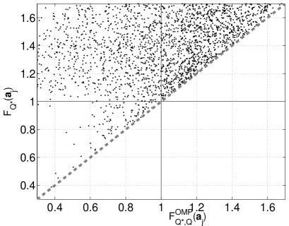
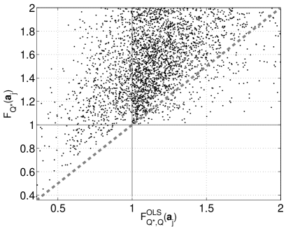
(a) $F_{{\mathcal{Q}}^{\star}}({\mathb{a}}_{j})$ vs $F_{{\mathcal{Q}}^{\star},{\mathcal{Q}}}^{\mathrm{OMP}}({\mathb{a}}_{j})$.	(b) $F_{{\mathcal{Q}}^{\star}}({\mathb{a}}_{j})$ vs $F_{{\mathcal{Q}}^{\star},{\mathcal{Q}}}^{\mathrm{OLS}}({\mathb{a}}_{j})$.
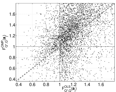
(c) $F_{{\mathcal{Q}}^{\star},{\mathcal{Q}}}^{\mathrm{OMP}}({\mathb{a}}_{j})$ vs $F_{{\mathcal{Q}}^{\star},{\mathcal{Q}}}^{\mathrm{OLS}}({\mathb{a}}_{j})$.

Figure 1: Comparison of the OMP and OLS exact recovery conditions. We draw 10.000 Gaussian dictionaries of size $100\times 11$ and set $k=10$ so that there is only one wrong atom ${\mathb{a}}_{j}$. $\mathcal{Q}$ is always set to the first atom (${\mathrm{Card}}\left[{\mathcal{Q}}\right]=1$). Plot of (a) $F_{{\mathcal{Q}}^{\star}}({\mathb{a}}_{j})$ vs $F_{{\mathcal{Q}}^{\star},{\mathcal{Q}}}^{\mathrm{OMP}}({\mathb{a}}_{j})$; (b) $F_{{\mathcal{Q}}^{\star}}({\mathb{a}}_{j})$ vs $F_{{\mathcal{Q}}^{\star},{\mathcal{Q}}}^{\mathrm{OLS}}({\mathb{a}}_{j})$; (c) $F_{{\mathcal{Q}}^{\star},{\mathcal{Q}}}^{\mathrm{OMP}}({\mathb{a}}_{j})$ vs $F_{{\mathcal{Q}}^{\star},{\mathcal{Q}}}^{\mathrm{OLS}}({\mathb{a}}_{j})$. For the last subfigure, we keep the trials for which $F_{{\mathcal{Q}}^{\star}}({\mathb{a}}_{j})\geqslant 1$.

IV-B1 There is no logical implication between the ERC-OMP and ERC-OLS conditions

We first investigate what is going on after the first iteration ($q=1$). We compare ERC-OMP(${\mathb{A}},{\mathcal{Q}}^{\star},{\mathcal{Q}}$) and ERC-OLS(${\mathb{A}},{\mathcal{Q}}^{\star},{\mathcal{Q}}$) for a common dictionary and given subsets ${\mathcal{Q}}\subsetneq{\mathcal{Q}}^{\star}$ with $q=1$. As the recovery conditions take the form “for all $j\notin{\mathcal{Q}}^{\star}$, $F_{{\mathcal{Q}}^{\star},{\mathcal{Q}}}^{\mathrm{Oxx}}({\mathb{a}}_{j})<1$”, it is sufficient to just consider the case where there is one wrong atom ${\mathb{a}}_{j}$ to study the logical implication between the ERC-OMP and ERC-OLS conditions. Therefore, in this paragraph, we consider undercomplete dictionaries $\mathb{A}$ with $k+1$ atoms. Testing ERC(${\mathb{A}},{\mathcal{Q}}^{\star}$), ERC-OMP(${\mathb{A}},{\mathcal{Q}}^{\star},{\mathcal{Q}}$) and ERC-OLS(${\mathb{A}},{\mathcal{Q}}^{\star},{\mathcal{Q}}$) amounts to evaluating $F_{{\mathcal{Q}}^{\star}}({\mathb{a}}_{j})$, $F_{{\mathcal{Q}}^{\star},{\mathcal{Q}}}^{\mathrm{OMP}}({\mathb{a}}_{j})$ and $F_{{\mathcal{Q}}^{\star},{\mathcal{Q}}}^{\mathrm{OLS}}({\mathb{a}}_{j})$ and comparing them to 1.

Fig. 1 is a scatter plot of the three criteria for 10.000 randomly Gaussian dictionaries $\mathb{A}$ of size $100\times 11$. The subset ${\mathcal{Q}}=\{1\}$ is systematically chosen as the first atom of $\mathb{A}$. Figs. 1(a,b) are in good agreement with Lemma 2: we verify that $F_{{\mathcal{Q}}^{\star},{\mathcal{Q}}}^{\mathrm{OMP}}({\mathb{a}}_{j})\leqslant F_{{\mathcal{Q}}^{\star}}({\mathb{a}}_{j})$ whether the ERC holds or not, and that $F_{{\mathcal{Q}}^{\star},{\mathcal{Q}}}^{\mathrm{OLS}}({\mathb{a}}_{j})\leqslant F_{{\mathcal{Q}}^{\star}}({\mathb{a}}_{j})$ systematically occurs only when $F_{{\mathcal{Q}}^{\star}}({\mathb{a}}_{j})<1$. On Fig. 1(c) displaying $F_{{\mathcal{Q}}^{\star},{\mathcal{Q}}}^{\mathrm{OMP}}({\mathb{a}}_{j})$ versus $F_{{\mathcal{Q}}^{\star},{\mathcal{Q}}}^{\mathrm{OLS}}({\mathb{a}}_{j})$, we only keep the trials for which $F_{{\mathcal{Q}}^{\star}}({\mathb{a}}_{j})\geqslant 1$, i.e., ERC(${\mathb{A}},{\mathcal{Q}}^{\star}$) does not hold. Since both south-east and north-west quarter planes are populated, we conclude that neither OMP nor OLS is uniformly better. To be more specific, when ERC-OMP(${\mathb{A}},{\mathcal{Q}}^{\star},{\mathcal{Q}}$) holds but ERC-OLS(${\mathb{A}},{\mathcal{Q}}^{\star},{\mathcal{Q}}$) does not, there exists an input ${\mathb{y}}\in{\mathrm{span}}({\mathb{A}}_{{\mathcal{Q}}^{\star}})$ for which OLS selects ${\mathcal{Q}}=\{1\}$ and then a wrong atom in the second iteration (Theorem 4). On the contrary, OMP is guaranteed to exactly recover this input according to Theorem 3. The same situation can occur when inverting the roles of OMP and OLS according to Corollary 2 and Theorem 3 (note that this analysis becomes more complex when ${\mathrm{Card}}\left[{\mathcal{Q}}\right]\geqslant 2$ since ERC-OMP(${\mathb{A}},{\mathcal{Q}}^{\star},{\mathcal{Q}}$) alone is not a necessary condition for OMP anymore; Theorem 5 also involves the assumption that $\mathcal{Q}$ is reachable).

We have compared ERC-OMP(${\mathb{A}},{\mathcal{Q}}^{\star},1$) and ERC-OLS(${\mathb{A}},{\mathcal{Q}}^{\star},1$), which take into account all the possible subsets of ${\mathcal{Q}}^{\star}$ of cardinality $1$. Again, we found that when ERC(${\mathb{A}},{\mathcal{Q}}^{\star}$) is not met, it can occur that ERC-OMP(${\mathb{A}},{\mathcal{Q}}^{\star},1$) holds while ERC-OLS(${\mathb{A}},{\mathcal{Q}}^{\star},1$) does not and vice versa.

IV-B2 Phase transition analysis for overcomplete random dictionaries

We now address the case of overcomplete dictionaries. Moreover, we study the dependence of the ERC-Oxx conditions with respect to the cardinalities $k$ and $q$ for $k>q\geqslant 2$ and we compare them for common problems (${\mathb{A}},{\mathcal{Q}}^{\star},{\mathcal{Q}}$).

Let us start with simple preliminary remarks. Because the ERC-Oxx(${\mathb{A}},{\mathcal{Q}}^{\star},{\mathcal{Q}}$) conditions take the form “for all $j\notin{\mathcal{Q}}^{\star}$, $F_{{\mathcal{Q}}^{\star},{\mathcal{Q}}}^{\mathrm{Oxx}}({\mathb{a}}_{j})<1$”, they are more often met when the dictionary is undercomplete (or when $m\approx n$) than in the overcomplete case: when the submatrix ${\mathb{A}}_{{\mathcal{Q}}^{\star}}$ gathering the true atoms is given, $\max_{j\notin{\mathcal{Q}}^{\star}}F_{{\mathcal{Q}}^{\star},{\mathcal{Q}}}^{\mathrm{Oxx}}({\mathb{a}}_{j})$ is obviously increasing when additional wrong atoms ${\mathb{a}}_{j}$ are incorporated, i.e., when $n$ is increasing. Additionally, we notice that for given $\mathb{A}$ and ${\mathcal{Q}}^{\star}$, $F_{{\mathcal{Q}}^{\star},{\mathcal{Q}}}^{\mathrm{OMP}}$ always decreases when ${\mathcal{Q}}$ is growing by definition of $F_{{\mathcal{Q}}^{\star},{\mathcal{Q}}}^{\mathrm{OMP}}$. This might not be the case of $F_{{\mathcal{Q}}^{\star},{\mathcal{Q}}}^{\mathrm{OLS}}$ for specific settings but it happens to be true in average for random dictionaries.

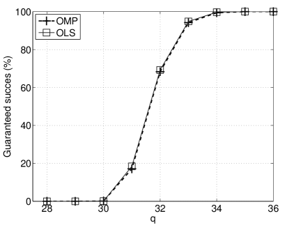
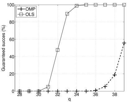
(a) Random dictionaries ($T=0$)	(b) Hybrid dictionaries ($T=10$)

Figure 2: Phase transition curves: for each $q<k$, we count the rate of trials where ERC-Oxx(${\mathb{A}},{\mathcal{Q}}^{\star},{\mathcal{Q}})$ is true, with ${\mathrm{Card}}\left[{\mathcal{Q}}\right]=q$. The dictionaries are of size $200\times 600$, $k$ is set to 40 and 1,000 Monte Carlo trials are performed.  (a) Randomly Gaussian dictionaries;  (b) Hybrid dictionaries with $T=10$.

In the following experiments, ${\mathcal{Q}}\subsetneq{\mathcal{Q}}^{\star}$ is gradually increased for fixed $\mathb{A}$ and ${\mathcal{Q}}^{\star}$, and we search for the first cardinality $q={\mathrm{Card}}\left[{\mathcal{Q}}\right]$ for which ERC-Oxx(${\mathb{A}},{\mathcal{Q}}^{\star},{\mathcal{Q}}$) is met. This allows us to define a “phase transition curve” [17, 28] which separates the $q$-values for which ERC-Oxx(${\mathb{A}},{\mathcal{Q}}^{\star},{\mathcal{Q}}$) is never met, and is always met. Examples of phase transition curves are given on Fig. 2 for random ($T=0$) and hybrid dictionaries ($T=10$). Fig. 2(a) shows that for $T=0$, the phase transition regime occurs in the same interval $q\in\{30,\ldots,34\}$ for both OMP and OLS and that the OMP and OLS curves are superimposed. On the contrary, for hybrid dictionaries (Fig. 2(b)), the mutual coherence increases and the OLS curve is significantly above the OMP curve. Thus, the guaranteed success for OLS occurs (in average) for an earlier iteration than for OMP. For larger values of $T$ (e.g., for $T=100$), the ERC-OMP condition is never met before $q=k-1$, and even for $q=k-1$, it is met for only $4~{}\%$ of trials.

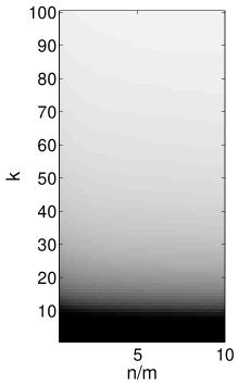
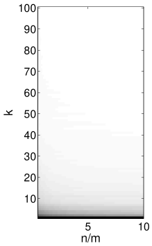
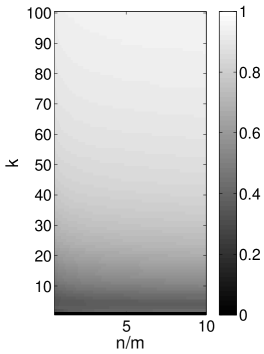
(a) OMP, $T=0$	(b) OLS, $T=0$	(c) OMP, $T=10$	(d) OLS, $T=10$

Figure 3: Phase transition diagrams for the ERC-Oxx(${\mathb{A}},{\mathcal{Q}}^{\star},{\mathcal{Q}}$) condition. The gray levels represent the ratio $[q]^{\mathrm{Oxx}}(m,n,k)/k\in[0,1]$. Averaging is done over 200 draws of dictionary $\mathb{A}$ and subset ${\mathcal{Q}}^{\star}$.   (a,b) Randomly Gaussian dictionaries of size $200\times n$ with $n\leqslant 2000$; (c,d) Hybrid dictionaries of same size, with $T=10$.

The experiment of Fig. 2 is repeated for many values of $k$ and dictionary sizes $m\times n$. For given $\mathb{A}$ and ${\mathcal{Q}}^{\star}$, let $q^{\mathrm{Oxx}}(m,n,k)$ denote the lowest value of $q={\mathrm{Card}}\left[{\mathcal{Q}}\right]$ for which ERC-Oxx(${\mathb{A}},{\mathcal{Q}}^{\star},{\mathcal{Q}})$ is true. For random and hybrid dictionaries, we perform 200 Monte Carlo simulations in which random matrices $\mathb{A}$ and subsets $({\mathcal{Q}}^{\star},{\mathcal{Q}})$ are drawn and we compute the average values of $q^{\mathrm{Oxx}}$, denoted by $[q]^{\mathrm{Oxx}}(m,n,k)$. This yields a phase transition diagram [12, 29] with the dictionary size (e.g., $n/m$) and the sparsity level $k$ in $x$- and $y$-axes, respectively. In this image, the gray levels represent the ratio $[q]^{\mathrm{Oxx}}(m,n,k)/k$ (see Fig. 3). Note that our phase transition diagrams are related to worst case recovery conditions, so better performance may be achieved by actually running Oxx for some simulated data $({\mathb{y}},{\mathb{A}})$ and testing whether the support ${\mathcal{Q}}^{\star}$ is found, where ${\mathb{y}}={\mathb{A}}{\mathb{x}}^{\star}$ and the unknown nonzero amplitudes in ${\mathb{x}}^{\star}$ are drawn according to a specific distribution.

A general comment regarding the results of Fig. 3 is that the ERC-Oxx conditions are satisfied early (for low values of $q/k$) when the unknown signal is highly sparse ($k$ is low) or when $n/m$ is low, i.e., when the dictionary is not highly overcomplete. The ratio $[q]^{\mathrm{Oxx}}(m,n,k)/k$ gradually grows with $k$ and $n/m$. Regarding the OMP vs OLS comparison, the phase diagrams obtained for OMP and OLS look very much alike for Gaussian dictionaries ($T=0$). On the contrary, we observe drastic differences in favor of OLS for hybrid dictionaries (Fig. 3(c,d)): $F_{{\mathcal{Q}}^{\star},{\mathcal{Q}}}^{\mathrm{OLS}}$ is significantly lower than $F_{{\mathcal{Q}}^{\star},{\mathcal{Q}}}^{\mathrm{OMP}}$.

We have performed similar tests for randomly uniform dictionaries (and hybrid dictionaries based on a randomly uniform process) and we draw conclusions similar to the Gaussian case. We have not encountered any situation where $F_{{\mathcal{Q}}^{\star},{\mathcal{Q}}}^{\mathrm{OMP}}$ is (in average) significantly lower than $F_{{\mathcal{Q}}^{\star},{\mathcal{Q}}}^{\mathrm{OLS}}$.

IV-B3 ERC-Oxx evaluation for sparse spike train deconvolution dictionaries

We reproduced the above experiments for the convolutive dictionary introduced in subsection IV-A. Since the dictionary is deterministic, only one trial is performed per cardinality ($m,n,k$). In each of the simulations hereafter, we set ${\mathcal{Q}}$ and ${\mathcal{Q}}^{\star}$ to contiguous atoms. This is the worst situation because contiguous atoms are the most highly correlated and exact support recovery may be more easily achieved if we impose a minimum distance between true atoms [30, 24]. The curves of Fig. 4 represent $F_{{\mathcal{Q}}^{\star},{\mathcal{Q}}}^{\mathrm{Oxx}}$ with respect to $q$ for some given $({\mathb{A}},{\mathcal{Q}}^{\star})$. It is noticeable that the OLS curve decreases much faster than the OMP curve, and that $F_{{\mathcal{Q}}^{\star},{\mathcal{Q}}}^{\mathrm{OMP}}$ remains huge even after a number of iterations. For all our trials where the true atoms strongly overlap, the ERC-OMP(${\mathb{A}},{\mathcal{Q}}^{\star},{\mathcal{Q}}$) condition is not met while ERC-OLS(${\mathb{A}},{\mathcal{Q}}^{\star},{\mathcal{Q}}$) may be fulfilled after a number of iterations which is, however, close to $k$. Moreover, we found that when $\sigma$ is large enough, $F_{{\mathcal{Q}}^{\star},{\mathcal{Q}}}^{\mathrm{OMP}}$ remains larger than 1 even for $q=k-1$, whereas the ERC-OLS condition is always met for $q=k-1$.

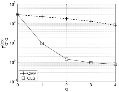
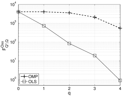
(a)	(b)

Figure 4: Curve representing $F_{{\mathcal{Q}}^{\star},{\mathcal{Q}}}^{\mathrm{Oxx}}$ as a function of $q={\mathrm{Card}}\left[{\mathcal{Q}}\right]$ for the Gaussian deconvolution problem. ${\mathcal{Q}}^{\star}$ is fixed and ${\mathcal{Q}}\subsetneq{\mathcal{Q}}^{\star}$ is gradually growing. ${\mathcal{Q}}^{\star}$ and ${\mathcal{Q}}$ are formed of the first $k=5$ and the first $q$ atoms, respectively with $q<k$.  (a) The Gaussian impulse response is of width $\sigma=50$ and the dictionary is of size $3000\times 2710$.   (b) $\sigma$ is set to 10, and the dictionary is of size $1000\times 4940$.

Empirical evaluations of the ERC condition for sparse spike train deconvolution was already done in [27]. In [27, 30, 24], a stronger sufficient condition than the ERC is evaluated for convolutive dictionaries. It is a sufficient (but not necessary) exact recovery condition that is easier to compute than the ERC because it does not require any matrix inversion, and only relies on inner products between the dictionary atoms (see [31, Lemma 3] for further details). In [27, 30], it was pointed out that the ERC condition is usually not fulfilled for convolutive dictionaries, but when the true atoms are enough spaced, successful recovery is guaranteed to occur. Our study can be seen as an alternative analysis to [27, 30, 24] in which no minimal distance constraint is imposed.

IV-C Examples where the bad recovery condition of OMP is met

We exhibit several situations in which the BRC-OMP(${\mathb{A}},{\mathcal{Q}}^{\star}$) condition may be fulfilled. This allows us to distinguish OMP from OLS as we know that under regular conditions, any subset ${\mathcal{Q}}^{\star}$ is reachable using OLS at least for some input in ${\mathrm{span}}({\mathb{A}}_{{\mathcal{Q}}^{\star}})$ (Lemma 3). The first situation is a simple dictionary with four atoms, some of which being strongly correlated. For this example, we show a stronger result than the BRC: there exists a subset ${\mathcal{Q}}^{\star}$ which is not reachable for any ${\mathb{y}}\in{\mathrm{span}}({\mathb{A}}_{{\mathcal{Q}}^{\star}})$, but not even for any ${\mathb{y}}\in{\mathbbm{R}}^{m}$. The other examples involve the random, hybrid and deterministic dictionaries introduced in subsection IV-A.

IV-C1 Example with four atoms

Example 1

Consider the simple dictionary

$${\mathb{A}} =\left[{\begin{array}[]{rrrr}\cos\theta_{1}&\cos\theta_{1}&0&0\\ -\sin\theta_{1}&\sin\theta_{1}&\cos\theta_{2}&\cos\theta_{2}\\ 0&0&\sin\theta_{2}&-\sin\theta_{2}\end{array}}\right]$$

with ${\mathcal{Q}}^{\star}=\{1,2\}$. Set $\theta_{2}$ to an arbitrary value in $(0,\pi/2)$. When $\theta_{1}\neq 0$ is close enough to 0, BRC-OMP(${\mathb{A}},{\mathcal{Q}}^{\star}$) is met. Moreover, OMP cannot reach ${\mathcal{Q}}^{\star}$ in two iterations for any ${\mathb{y}}\in{\mathbbm{R}}^{3}$ (specifically, when ${\mathb{y}}\in{\mathbbm{R}}^{3}$ is proportional to neither ${\mathb{a}}_{1}$ nor ${\mathb{a}}_{2}$, ${\mathb{a}}_{3}$ or ${\mathb{a}}_{4}$ is selected in the first two iterations).

Proof:

We first prove that the BRC condition is met by calculating the factors $F_{{\mathcal{Q}}^{\star},\{1\}}^{\mathrm{OMP}}({\mathb{a}}_{j})$ and $F_{{\mathcal{Q}}^{\star},\{2\}}^{\mathrm{OMP}}({\mathb{a}}_{j})$ for $j\in\{3,4\}$. Let us start with $F_{{\mathcal{Q}}^{\star},\{1\}}^{\mathrm{OMP}}({\mathb{a}}_{j})$.

The simple projection calculation $\tilde{{\mathb{a}}}_{i}={\mathb{a}}_{i}-\langle{\mathb{a}}_{i},{\mathb{a}}_{1}\rangle{\mathb{a}}_{1}$ (the tilde notation implicitly refers to ${\mathcal{Q}}=\{1\}$) leads to:

$$\tilde{{\mathb{a}}}_{2}=\sin(2\theta_{1})\left[\begin{array}[]{@{}c@{}}\sin\theta_{1}\\ \cos\theta_{1}\\ 0\end{array}\right],\;\;\tilde{{\mathb{a}}}_{3}=\left[\begin{array}[]{@{}c@{}}\sin\theta_{1}\cos\theta_{1}\cos\theta_{2}\\ \cos^{2}\theta_{1}\cos\theta_{2}\\ \sin\theta_{2}\end{array}\right]\;\;\textrm{and}\;\;\tilde{{\mathb{a}}}_{4}=\left[\begin{array}[]{@{}c@{}}\sin\theta_{1}\cos\theta_{1}\cos\theta_{2}\\ \cos^{2}\theta_{1}\cos\theta_{2}\\ -\sin\theta_{2}\end{array}\right].$$

According to (11), the OMP recovery factor reads for $j\in\{3,4\}$:

$$F_{{\mathcal{Q}}^{\star},\{1\}}^{\mathrm{OMP}}({\mathb{a}}_{j}) =\frac{|\langle\tilde{{\mathb{a}}}_{2},\tilde{{\mathb{a}}}_{j}\rangle|}{\|\tilde{{\mathb{a}}}_{2}\|^{2}}=\frac{|\cos\theta_{1}\cos\theta_{2}|}{|\sin(2\theta_{1})|}$$ (12)

given that $\|\tilde{{\mathb{a}}}_{2}\|=|\sin(2\theta_{1})|$ and $|\langle\tilde{{\mathb{a}}}_{2},\tilde{{\mathb{a}}}_{3}\rangle|=|\langle\tilde{{\mathb{a}}}_{2},\tilde{{\mathb{a}}}_{4}\rangle|=\|\tilde{{\mathb{a}}}_{2}\|\,|\cos\theta_{1}\cos\theta_{2}|$. $F_{{\mathcal{Q}}^{\star},\{2\}}^{\mathrm{OMP}}({\mathb{a}}_{j})$ can be obtained symmetrically by replacing $\theta_{1}$ by $-\theta_{1}$ in (12). Thus, we have $F_{{\mathcal{Q}}^{\star},\{2\}}^{\mathrm{OMP}}({\mathb{a}}_{j})=F_{{\mathcal{Q}}^{\star},\{1\}}^{\mathrm{OMP}}({\mathb{a}}_{j})$. It follows that the left hand-side of the BRC-OMP(${\mathb{A}},{\mathcal{Q}}^{\star}$) condition reads (12) and tends towards $+\infty$ when $\theta_{1}$ tends towards 0. Therefore, BRC-OMP(${\mathb{A}},{\mathcal{Q}}^{\star}$) is met when $|\theta_{1}|$ is small enough.

Figure 5: Example 1: drawing of the plane ${\mathrm{span}}({\mathb{a}}_{1})^{\perp}$. The tilde notation refers to the subset ${\mathcal{Q}}=\{1\}$. When $\theta_{1}$ is close to 0, $\tilde{{\mathb{a}}}_{2}$ is of very small norm since ${\mathb{a}}_{2}$ is almost equal to ${\mathb{a}}_{1}$, while ${\mathb{a}}_{3}$ and ${\mathb{a}}_{4}$, which are almost orthogonal to ${\mathb{a}}_{1}$, yield projections $\tilde{{\mathb{a}}}_{3}$ and $\tilde{{\mathb{a}}}_{4}$ that are almost of unit norm. The angles $(\tilde{{\mathb{a}}}_{2},\tilde{{\mathb{a}}}_{3})$ and $(\tilde{{\mathb{a}}}_{2},\tilde{{\mathb{a}}}_{4})$ tend to $\theta_{2}$ and $-\theta_{2}$ when $\theta_{1}\rightarrow 0$. The bullet and square points correspond to positions $\mathb{r}$ satisfying $|\langle{\mathb{r}},\tilde{{\mathb{a}}}_{2}\rangle|\geqslant|\langle{\mathb{r}},\tilde{{\mathb{a}}}_{3}\rangle|$ and $|\langle{\mathb{r}},\tilde{{\mathb{a}}}_{2}\rangle|\geqslant|\langle{\mathb{r}},\tilde{{\mathb{a}}}_{4}\rangle|$, respectively. The central directions of these two cones are orthogonal to $\tilde{{\mathb{a}}}_{3}$ and $\tilde{{\mathb{a}}}_{4}$, respectively (dashed lines). Both cones only intersect at ${\mathb{r}}={\mathbf{0}}$, therefore OMP cannot successively select ${\mathb{a}}_{1}$ and ${\mathb{a}}_{2}$ in the first two iterations.

To show that ${\mathcal{Q}}^{\star}$ is not reachable for any ${\mathb{y}}\in{\mathbbm{R}}^{3}$, let us assume that OMP selects a true atom in the first iteration. Because there is a symmetry between ${\mathb{a}}_{1}$ and ${\mathb{a}}_{2}$, we can assume without loss of generality that ${\mathb{a}}_{1}$ is selected. Then, the data residual ${\mathb{r}}$ after the first iteration lies in ${\mathrm{span}}({\mathb{a}}_{1})^{\perp}$ which is of dimension 2. We show using geometrical arguments, that ${\mathb{a}}_{2}$ cannot be selected in the second iteration for any ${\mathb{r}}\in{\mathrm{span}}({\mathb{a}}_{1})^{\perp}\backslash\{{\mathbf{0}}\}$. We refer the reader to Fig. 5 for a 2D display of the projected atoms in the plane ${\mathrm{span}}({\mathb{a}}_{1})^{\perp}$.

Let $\mathcal{C}$ denote the set of points ${\mathb{r}}\in{\mathbbm{R}}^{2}$ satisfying $|\langle{\mathb{r}},\tilde{{\mathb{a}}}_{2}\rangle|\geqslant|\langle{\mathb{r}},\tilde{{\mathb{a}}}_{3}\rangle|$. ${\mathb{r}}\in{\mathcal{C}}$ if and only if there exist $(\varepsilon_{2},\varepsilon_{3})\in\{-1,1\}^{2}$ such that $\varepsilon_{2}\langle{\mathb{r}},\tilde{{\mathb{a}}}_{2}\rangle\geqslant\varepsilon_{3}\langle{\mathb{r}},\tilde{{\mathb{a}}}_{3}\rangle\geqslant 0$, i.e.,

$$\langle{\mathb{r}},\varepsilon_{2}\tilde{{\mathb{a}}}_{2}-\varepsilon_{3}\tilde{{\mathb{a}}}_{3}\rangle\geqslant 0\;\;\mathrm{and}\;\;\langle{\mathb{r}},\varepsilon_{3}\tilde{{\mathb{a}}}_{3}\rangle\geqslant 0.$$ (13)

For each sign pattern $(\varepsilon_{2},\varepsilon_{3})$, (13) yields a 2D half cone defined as the intersection of two half-planes delimited by the directions which are orthogonal to $\tilde{{\mathb{a}}}_{3}$ and $\varepsilon_{2}\tilde{{\mathb{a}}}_{2}-\varepsilon_{3}\tilde{{\mathb{a}}}_{3}$. Moreover, the opposite sign pattern $(-\varepsilon_{2},-\varepsilon_{3})$ yields the remaining part of the same 2D cone. Consequently, the four possible sign patterns $(\varepsilon_{2},\varepsilon_{3})\in\{-1,1\}^{2}$ yield both cones delimited by the orthogonal directions to $\tilde{{\mathb{a}}}_{3}$ and $\tilde{{\mathb{a}}}_{2}+\tilde{{\mathb{a}}}_{3}$, and to $\tilde{{\mathb{a}}}_{3}$ and $-\tilde{{\mathb{a}}}_{2}+\tilde{{\mathb{a}}}_{3}$, respectively. Because these cones are adjacent, their union $\mathcal{C}$ is the cone delimited by the orthogonal directions to $\tilde{{\mathb{a}}}_{3}+\tilde{{\mathb{a}}}_{2}$ and $\tilde{{\mathb{a}}}_{3}-\tilde{{\mathb{a}}}_{2}$ (plain lines in the south-east and north-west directions in Fig. 5). Similarly, the condition $|\langle{\mathb{r}},\tilde{{\mathb{a}}}_{2}\rangle|\geqslant|\langle{\mathb{r}},\tilde{{\mathb{a}}}_{4}\rangle|$ yields another 2D cone whose central direction is orthogonal to $\tilde{{\mathb{a}}}_{4}$. When $\theta_{1}$ is close to 0, both cones only intersect at ${\mathb{r}}={\mathbf{0}}$ (since their inner angle tends towards 0), thus

$$\forall{\mathb{r}}\in{\mathbbm{R}}^{2}\backslash\{{\mathbf{0}}\},\;|\langle{\mathb{r}},\tilde{{\mathb{a}}}_{2}\rangle|<\max(|\langle{\mathb{r}},\tilde{{\mathb{a}}}_{3}\rangle|,|\langle{\mathb{r}},\tilde{{\mathb{a}}}_{4}\rangle|).$$

We conclude that ${\mathb{a}}_{2}$ cannot be selected in the second iteration according to the OMP rule (1). ∎

IV-C2 Numerical simulation of the BRC condition

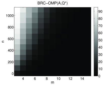
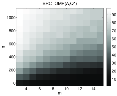
(a) Gaussian dictionaries	(b) Hybrid dictionaries ($T=10$)

Figure 6: Evaluation of the bad recovery condition BRC-OMP(${\mathb{A}},{\mathcal{Q}}^{\star}$) for randomly Gaussian (a) and hybrid (b) dictionaries of various sizes $(m,n)$. 1,000 trials are performed per dictionary size, and ${\mathcal{Q}}^{\star}$ is always set to the first two atoms ($k=2$). The gray levels correspond to the rate of guaranteed failure, i.e., the proportion of trials where BRC-OMP(${\mathb{A}},{\mathcal{Q}}^{\star}$) holds.

We test the BRC-OMP condition for various dictionary sizes ($m,n$) for the random, hybrid and convolutive dictionaries introduced in subsection IV-A. The average results related to the random and hybrid dictionaries are gathered in Fig. 6 in the case $k=2$. For randomly Gaussian dictionaries, we observe that the BRC-OMP condition may be met for strongly overcomplete dictionaries, i.e., when $n\gg m$ (Fig. 6 (a)). In the special case $k=2$, it is noticeable that OLS performs at least as well as OMP whether the BRC condition if fulfilled or not: when the first iteration (common to both algorithms) has succeeded, OLS cannot fail according to Theorem 6 while OMP is guaranteed to fail in cases where the BRC holds. For the hybrid dictionaries, the BRC condition is more frequently met when the dictionary is moderately overcomplete, i.e., for large values of $m/n$. This result is in coherence with our evaluations of the ERC-Oxx condition (see, e.g., Fig. 3(c)) which are more rarely met for hybrid dictionary than for random dictionaries.

We performed similar tests for the sparse spike train deconvolution problem with a Gaussian impulse response of width $\sigma$, and with $k=2$ (the true atoms are contiguous, thus they are strongly correlated). We repeated the simulation of Fig. 6 for various sizes $m\approx n$ and various widths $\sigma$, and we found that whatever $(m,n)$, the BRC condition is always met for $\sigma\geqslant 1.5$ and never met when $\sigma\leqslant 1.4$. The images of Fig. 6 thus become uniformly white and uniformly black, respectively. To be more specific, the value of the left hand-side of the BRC-OMP(${\mathb{A}},{\mathcal{Q}}^{\star}$) condition gradually increases with $\sigma$, e.g., this value reaches 10, 35 and 48 for $\sigma=10$, 20 and 50, respectively for dictionaries of size $m\approx n$, with $m=3000$. This result is in coherence with that of Fig. 4 which already indicated that the $F_{{\mathcal{Q}}^{\star},{\mathcal{Q}}}^{\mathrm{OMP}}$ factor becomes huge for convolutive problems with strongly correlated atoms.

Note that when ${\mathcal{Q}}^{\star}$ does not involve contiguous atoms but “spaced atoms” which are less correlated, the bad recovery condition are met for larger values of $\sigma$: denoting by $\Delta$ the minimum distance between two true atoms, the lowest $\Delta$ value for which the BRC is met turns out to be an increasing affine function of $\sigma$. Similar empirical studies were done in [27] for the exact recovery condition for spaced atoms, and in [27, 24] for the weak exact recovery condition of [31, Lemma 3]. In particular, the numerical simulations in [24] for the Gaussian deconvolution problem demonstrate that the latter condition is met for larger $\sigma$’s when the minimum distance between true atoms is increased and the limit $\Delta$ value corresponding to the phase transition is also an affine function of $\sigma$. Our bad recovery condition results are thus a complement to those of [24].

V Conclusions

Our first contribution is an original analysis of OLS based on the extension of the ERC condition. We showed that when the ERC holds, OLS is guaranteed to yield an exact support recovery. Although OLS has been acknowledged in several communities for two decades, such a theoretical analysis was lacking. Our second contribution is a parallel study of OMP and OLS when a number of iterations have been performed and true atoms have been selected. We found that neither OMP nor OLS is uniformly better. In particular, we showed using randomly Gaussian dictionaries that when the ERC is not met but the first iteration (which is common to OMP and OLS) selects a true atom, there are counter-examples for which OMP is guaranteed to yield an exact support recovery while OLS does not, and vice versa.

Finally, several elements of analysis suggest that OLS behaves better than OMP. First, any subset $\mathcal{Q}$ can be reached by OLS using some input in ${\mathrm{span}}({\mathb{A}}_{\mathcal{Q}})$ while for some dictionaries, it may occur that some subsets are never reached by OMP for any ${\mathb{y}}\in{\mathbbm{R}}^{m}$. In other words, OLS has a stronger capability of exploration. Secondly, when all true atoms except one have been found by OLS and no wrong selection occurred, OLS is guaranteed to find the last true atom in the following iteration while OMP may fail.

For problems in which the dictionary is far from orthogonal and some dictionary atoms are strongly correlated, we found in our experiments that the OLS recovery condition might be met after some iterations while the OMP recovery condition is rarely met. We did not encounter the opposite situation where the OMP recovery condition is frequently met after fewer iterations than the OLS condition. Moreover, guaranteed failure of OMP may occur more often when the dictionary coherence is large. These results are in coherence with empirical studies reporting that OLS usually outperforms OMP at the price of a larger numerical cost [9, 11]. In our experience, OLS yields a residual error which may be by far lower than that of OMP after the same number of iterations [25]. Moreover, it performs better support recoveries in terms of ratio between the number of good detections and of false alarms [26].

Appendix A Necessary and sufficient conditions of exact recovery for OMP and OLS

This appendix includes the complete analysis of our OMP and OLS recovery conditions.

A-A Sufficient conditions

We show that when Oxx happens to select true atoms during its early iterations, it is guaranteed to recover the whole unknown support in the subsequent iterations when the ERC-Oxx(${\mathb{A}},{\mathcal{Q}}^{\star},{\mathcal{Q}}$) condition is fulfilled. We establish Theorem 3 whose direct consequence is Theorem 2 stating that when ERC(${\mathb{A}},{\mathcal{Q}}^{\star}$) holds, OLS is guaranteed to succeed.

A-A1 ERC-Oxx are sufficient recovery conditions at a given iteration

We follow the analysis of [1, Theorem 3.1] to extend Tropp’s exact recovery condition to a sufficient condition dedicated to the $(q+1)$-th iteration of Oxx.

Lemma 4

Assume that ${\mathb{A}}_{{\mathcal{Q}}^{\star}}$ is full rank. If Oxx with ${\mathb{y}}\in{\mathrm{span}}({\mathb{A}}_{{\mathcal{Q}}^{\star}})$ as input selects $q$ true atoms ${\mathcal{Q}}\subsetneq{\mathcal{Q}}^{\star}$ and ERC-Oxx(${\mathb{A}},{\mathcal{Q}}^{\star},{\mathcal{Q}}$) holds, then the $(q+1)$-th iteration of Oxx selects a true atom.

Proof:

According to the selection rule (1)-(2), Oxx selects a true atom at iteration $(q+1)$ if and only if

$$\phi({\mathb{r}}_{\mathcal{Q}})\triangleq\frac{\max_{i\notin{\mathcal{Q}}^{\star}}|\langle{\mathb{r}}_{\mathcal{Q}},\tilde{{\mathb{c}}}_{i}\rangle|}{\max_{i\in{\mathcal{Q}}^{\star}\backslash{\mathcal{Q}}}|\langle{\mathb{r}}_{\mathcal{Q}},\tilde{{\mathb{c}}}_{i}\rangle|}<1.$$ (14)

Let us gather the vectors $\tilde{{\mathb{c}}}_{i}$ indexed by $i\notin{\mathcal{Q}}^{\star}$ and $i\in{\mathcal{Q}}^{\star}\backslash{\mathcal{Q}}$ in two matrices $\tilde{{\mathb{C}}}_{\bullet\backslash{\mathcal{Q}}^{\star}}$ and $\tilde{{\mathb{C}}}_{{\mathcal{Q}}^{\star}\backslash{\mathcal{Q}}}$ of dimensions $m\times(n-k)$ and $m\times(k-q)$, respectively where the notation $\bullet$ stands for all indices $i\in\{1,\ldots,n\}$. The condition (14) rereads:

$$\phi({\mathb{r}}_{\mathcal{Q}})=\frac{\|\tilde{{\mathb{C}}}_{\bullet\backslash{\mathcal{Q}}^{\star}}^{t}{\mathb{r}}_{\mathcal{Q}}\|_{\infty}}{\|\tilde{{\mathb{C}}}_{{\mathcal{Q}}^{\star}\backslash{\mathcal{Q}}}^{t}{\mathb{r}}_{\mathcal{Q}}\|_{\infty}}<1.$$

Following Tropp’s analysis, we re-arrange the vector ${\mathb{r}}_{\mathcal{Q}}$ occurring in the numerator. Since ${\mathb{r}}_{\mathcal{Q}}={\mathb{P}}_{{\mathcal{Q}}}^{\perp}{\mathb{y}}$ and ${\mathb{y}}\in{\mathrm{span}}({\mathb{A}}_{{\mathcal{Q}}^{\star}})$, ${\mathb{r}}_{\mathcal{Q}}\in{\mathrm{span}}(\tilde{{\mathb{A}}}_{{\mathcal{Q}}^{\star}\backslash{\mathcal{Q}}})={\mathrm{span}}(\tilde{{\mathb{C}}}_{{\mathcal{Q}}^{\star}\backslash{\mathcal{Q}}})$. We rewrite ${\mathb{r}}_{\mathcal{Q}}$ as $\tilde{{\mathb{P}}}_{{\mathcal{Q}}^{\star}\backslash{\mathcal{Q}}}{\mathb{r}}_{\mathcal{Q}}$ where $\tilde{{\mathb{P}}}_{{\mathcal{Q}}^{\star}\backslash{\mathcal{Q}}}$ stands for the orthogonal projector on ${\mathrm{span}}(\tilde{{\mathb{C}}}_{{\mathcal{Q}}^{\star}\backslash{\mathcal{Q}}})$: $\tilde{{\mathb{P}}}_{{\mathcal{Q}}^{\star}\backslash{\mathcal{Q}}}=\tilde{{\mathb{P}}}_{{\mathcal{Q}}^{\star}\backslash{\mathcal{Q}}}^{t}=\bigl{(}\tilde{{\mathb{C}}}_{{\mathcal{Q}}^{\star}\backslash{\mathcal{Q}}}\tilde{{\mathb{C}}}_{{\mathcal{Q}}^{\star}\backslash{\mathcal{Q}}}^{\dagger}\bigr{)}^{t}$. $\phi({\mathb{r}}_{\mathcal{Q}})$ rereads

$$\phi({\mathb{r}}_{\mathcal{Q}})=\frac{\|\bigl{(}\tilde{{\mathb{C}}}_{{\mathcal{Q}}^{\star}\backslash{\mathcal{Q}}}^{\dagger}\tilde{{\mathb{C}}}_{\bullet\backslash{\mathcal{Q}}^{\star}}\bigr{)}^{t}\tilde{{\mathb{C}}}_{{\mathcal{Q}}^{\star}\backslash{\mathcal{Q}}}^{t}{\mathb{r}}_{\mathcal{Q}}\|_{\infty}}{\|\tilde{{\mathb{C}}}_{{\mathcal{Q}}^{\star}\backslash{\mathcal{Q}}}^{t}{\mathb{r}}_{\mathcal{Q}}\|_{\infty}}.$$

This expression can obviously be majorized using the matrix norm:

$$\phi({\mathb{r}}_{\mathcal{Q}})\leqslant\|\bigl{(}\tilde{{\mathb{C}}}_{{\mathcal{Q}}^{\star}\backslash{\mathcal{Q}}}^{\dagger}\tilde{{\mathb{C}}}_{\bullet\backslash{\mathcal{Q}}^{\star}}\bigr{)}^{t}\|_{\infty,\infty}.$$ (15)

Since the $\ell_{\infty}$ norm of a matrix is equal to the $\ell_{1}$ norm of its transpose and $\|\,.\,\|_{1,1}$ equals the maximum column sum of the absolute value of its argument [1, Theorem 3.1], the upper bound of (15) rereads

$$\max_{j\notin{\mathcal{Q}}^{\star}}\|\tilde{{\mathb{C}}}_{{\mathcal{Q}}^{\star}\backslash{\mathcal{Q}}}^{\dagger}\tilde{{\mathb{c}}}_{j}\|_{1}=\max_{j\notin{\mathcal{Q}}^{\star}}F_{{\mathcal{Q}}^{\star},{\mathcal{Q}}}^{\mathrm{Oxx}}({\mathb{a}}_{j})$$

according to Lemma 1. By definition of ERC-Oxx(${\mathb{A}},{\mathcal{Q}}^{\star},{\mathcal{Q}}$), this upper bound is lower than 1 thus $\phi({\mathb{r}}_{\mathcal{Q}})<1$. ∎

A-A2 Recursive expression of the ERC-Oxx formulas

We elaborate recursive expressions of $F_{{\mathcal{Q}}^{\star},{\mathcal{Q}}}^{\mathrm{Oxx}}({\mathb{a}}_{j})$ when $\mathcal{Q}$ is increased by one element resulting in the new subset ${\mathcal{Q}}^{\prime}\subsetneq{\mathcal{Q}}^{\star}$ (here, we do not consider the case where ${\mathcal{Q}}^{\prime}={\mathcal{Q}}^{\star}$ since $F_{{\mathcal{Q}}^{\star},{\mathcal{Q}}^{\star}}^{\mathrm{Oxx}}({\mathb{a}}_{j})$ is not properly defined, (4) and (5) being empty sums). We will use the notation ${\mathcal{Q}}^{\prime}={\mathcal{Q}}\cup\{\ell\}$ where $\ell\in{\mathcal{Q}}^{\star}\backslash{\mathcal{Q}}$. To avoid any confusion, $\tilde{{\mathb{a}}}_{i}$ will be systematically replaced by $\tilde{{\mathb{a}}}_{i}^{{\mathcal{Q}}}$ and $\tilde{{\mathb{a}}}_{i}^{{\mathcal{Q}}^{\prime}}$ to express the dependence upon $\mathcal{Q}$ and ${\mathcal{Q}}^{\prime}$, respectively. In the same way, $\tilde{{\mathb{b}}}_{i}$ will be replaced by $\tilde{{\mathb{b}}}_{i}^{{\mathcal{Q}}}$ or $\tilde{{\mathb{b}}}_{i}^{{\mathcal{Q}}^{\prime}}$ but for simplicity, we will keep the matrix notations $\tilde{{\mathb{B}}}_{{\mathcal{Q}}^{\star}\backslash{\mathcal{Q}}}$ and $\tilde{{\mathb{B}}}_{{\mathcal{Q}}^{\star}\backslash{\mathcal{Q}}^{\prime}}$ without superscript, $\tilde{}$ referring to $\mathcal{Q}$ and ${\mathcal{Q}}^{\prime}$, respectively.

Let us first link $\tilde{{\mathb{b}}}_{i}^{{\mathcal{Q}}}$ to $\tilde{{\mathb{b}}}_{i}^{{\mathcal{Q}}^{\prime}}$ when $\tilde{{\mathb{a}}}_{i}^{{\mathcal{Q}}^{\prime}}\neq{\mathbf{0}}$.

Lemma 5

Assume that ${\mathb{A}}_{{\mathcal{Q}}^{\prime}}$ is full rank and ${\mathcal{Q}}^{\prime}={\mathcal{Q}}\cup\{\ell\}\subsetneq{\mathcal{Q}}^{\star}$. Then, ${\mathrm{span}}({\mathb{A}}_{{\mathcal{Q}}})^{\perp}$ is the orthogonal direct sum of the subspaces ${\mathrm{span}}({\mathb{A}}_{{\mathcal{Q}}^{\prime}})^{\perp}$ and ${\mathrm{span}}(\tilde{{\mathb{a}}}_{\ell}^{\mathcal{Q}})$, and the normalized projection of any atom ${\mathb{a}}_{i}\notin{\mathrm{span}}({\mathb{A}}_{{\mathcal{Q}}^{\prime}})$ takes the form:

$$\tilde{{\mathb{b}}}_{i}^{{\mathcal{Q}}} =\eta_{i}^{{\mathcal{Q}},{\mathcal{Q}}^{\prime}}\tilde{{\mathb{b}}}_{i}^{{\mathcal{Q}}^{\prime}}+\chi_{i}^{{\mathcal{Q}},{\mathcal{Q}}^{\prime}}\tilde{{\mathb{b}}}_{\ell}^{{\mathcal{Q}}}$$ (16)

where

$$\eta_{i}^{{\mathcal{Q}},{\mathcal{Q}}^{\prime}} =\frac{\bigl{\|}\tilde{{\mathb{a}}}_{i}^{{\mathcal{Q}}^{\prime}}\bigr{\|}}{\bigl{\|}\tilde{{\mathb{a}}}_{i}^{{\mathcal{Q}}}\bigr{\|}}\,\in(0,1],$$ (17)

$$\chi_{i}^{{\mathcal{Q}},{\mathcal{Q}}^{\prime}} =\langle\tilde{{\mathb{b}}}_{i}^{{\mathcal{Q}}},\tilde{{\mathb{b}}}_{\ell}^{{\mathcal{Q}}}\rangle,$$ (18)

$$\bigl{(}\eta_{i}^{{\mathcal{Q}},{\mathcal{Q}}^{\prime}}\bigr{)}^{2} +\bigl{(}\chi_{i}^{{\mathcal{Q}},{\mathcal{Q}}^{\prime}}\bigr{)}^{2}=1.$$ (19)

Proof:

Since ${\mathcal{Q}}\subsetneq{\mathcal{Q}}^{\prime}$, we have ${\mathrm{span}}({\mathb{A}}_{{\mathcal{Q}}^{\prime}})^{\perp}\subseteq{\mathrm{span}}({\mathb{A}}_{{\mathcal{Q}}})^{\perp}$. Because ${\mathb{A}}_{{\mathcal{Q}}^{\prime}}$ is full rank, ${\mathrm{span}}({\mathb{A}}_{{\mathcal{Q}}^{\prime}})^{\perp}$ and ${\mathrm{span}}({\mathb{A}}_{{\mathcal{Q}}})^{\perp}$ are of consecutive dimensions. Moreover, $\tilde{{\mathb{a}}}_{\ell}^{\mathcal{Q}}={\mathb{a}}_{\ell}-{\mathb{P}}_{{\mathcal{Q}}}{\mathb{a}}_{\ell}\in{\mathrm{span}}({\mathb{A}}_{{\mathcal{Q}}^{\prime}})\cap{\mathrm{span}}({\mathb{A}}_{{\mathcal{Q}}})^{\perp}$, and $\tilde{{\mathb{a}}}_{\ell}^{\mathcal{Q}}\neq{\mathbf{0}}$ since ${\mathb{A}}_{{\mathcal{Q}}^{\prime}}$ is full rank. As a vector of ${\mathrm{span}}({\mathb{A}}_{{\mathcal{Q}}^{\prime}})$, $\tilde{{\mathb{a}}}_{\ell}^{\mathcal{Q}}$ is orthogonal to ${\mathrm{span}}({\mathb{A}}_{{\mathcal{Q}}^{\prime}})^{\perp}$. It follows that ${\mathrm{span}}(\tilde{{\mathb{a}}}_{\ell}^{\mathcal{Q}})$ is the orthogonal complement of ${\mathrm{span}}({\mathb{A}}_{{\mathcal{Q}}^{\prime}})^{\perp}$ in ${\mathrm{span}}({\mathb{A}}_{{\mathcal{Q}}})^{\perp}$.

The orthogonal decomposition of $\tilde{{\mathb{a}}}_{i}={\mathb{P}}_{{\mathcal{Q}}}^{\perp}{\mathb{a}}_{i}$ reads:

$$\tilde{{\mathb{a}}}_{i}^{{\mathcal{Q}}} =\tilde{{\mathb{a}}}_{i}^{{\mathcal{Q}}^{\prime}}+\langle\tilde{{\mathb{a}}}_{i}^{{\mathcal{Q}}},\tilde{{\mathb{b}}}_{\ell}^{\mathcal{Q}}\rangle\tilde{{\mathb{b}}}_{\ell}^{\mathcal{Q}}$$

since $\tilde{{\mathb{b}}}_{\ell}^{\mathcal{Q}}$ is of unit norm. Replacing $\tilde{{\mathb{a}}}_{i}^{{\mathcal{Q}}}=\|\tilde{{\mathb{a}}}_{i}^{{\mathcal{Q}}}\|\,\tilde{{\mathb{b}}}_{i}^{{\mathcal{Q}}}$ and $\tilde{{\mathb{a}}}_{i}^{{\mathcal{Q}}^{\prime}}=\|\tilde{{\mathb{a}}}_{i}^{{\mathcal{Q}}^{\prime}}\|\,\tilde{{\mathb{b}}}_{i}^{{\mathcal{Q}}^{\prime}}$ yields (16)-(18). Pythagoras’ theorem yields (19). The assumption ${\mathb{a}}_{i}\notin{\mathrm{span}}({\mathb{A}}_{{\mathcal{Q}}^{\prime}})$ implies that $\tilde{{\mathb{a}}}_{i}^{{\mathcal{Q}}^{\prime}}\neq{\mathbf{0}}$, then $\eta_{i}^{{\mathcal{Q}},{\mathcal{Q}}^{\prime}}>0$. ∎

Lemma 6

Assume that ${\mathb{A}}_{{\mathcal{Q}}^{\star}}$ is full rank. Let ${\mathcal{Q}}\subsetneq{\mathcal{Q}}^{\prime}\subsetneq{\mathcal{Q}}^{\star}$ with ${\mathcal{Q}}^{\prime}={\mathcal{Q}}\cup\{\ell\}$. Then, ${\mathrm{span}}(\tilde{{\mathb{B}}}_{{\mathcal{Q}}^{\star}\backslash{\mathcal{Q}}})$ is the orthogonal direct sum of ${\mathrm{span}}(\tilde{{\mathb{B}}}_{{\mathcal{Q}}^{\star}\backslash{\mathcal{Q}}^{\prime}})$ and ${\mathrm{span}}(\tilde{{\mathb{b}}}_{\ell}^{\mathcal{Q}})$.

Proof:

According to Corollary 3 in Appendix B, $\tilde{{\mathb{B}}}_{{\mathcal{Q}}^{\star}\backslash{\mathcal{Q}}}$ and $\tilde{{\mathb{B}}}_{{\mathcal{Q}}^{\star}\backslash{\mathcal{Q}}^{\prime}}$ are full rank matrices, thus their column spans are of consecutive cardinalities. Lemma 5 states that $\tilde{{\mathb{b}}}_{\ell}^{\mathcal{Q}}$ is orthogonal to ${\mathrm{span}}({\mathb{A}}_{{\mathcal{Q}}^{\prime}})^{\perp}$, thus it is orthogonal to $\tilde{{\mathb{b}}}_{i}^{{\mathcal{Q}}^{\prime}}\in{\mathrm{span}}({\mathb{A}}_{{\mathcal{Q}}^{\prime}})^{\perp}$ for all $i\in{\mathcal{Q}}^{\star}\backslash{\mathcal{Q}}^{\prime}$. ∎

We finally establish a link between $F_{{\mathcal{Q}}^{\star},{\mathcal{Q}}}^{\mathrm{Oxx}}({\mathb{a}}_{j})$ and $F_{{\mathcal{Q}}^{\star},{\mathcal{Q}}^{\prime}}^{\mathrm{Oxx}}({\mathb{a}}_{j})$. It is a simple recursive relation in the case of OMP. For OLS, we cannot directly relate the two quantities but we express $F_{{\mathcal{Q}}^{\star},{\mathcal{Q}}}^{\mathrm{OLS}}({\mathb{a}}_{j})=\bigl{\|}\tilde{{\mathb{B}}}_{{\mathcal{Q}}^{\star}\backslash{\mathcal{Q}}}^{\dagger}\tilde{{\mathb{b}}}_{j}^{\mathcal{Q}}\bigr{\|}_{1}$ with respect to $\tilde{{\mathb{B}}}_{{\mathcal{Q}}^{\star}\backslash{\mathcal{Q}}^{\prime}}^{\dagger}\tilde{{\mathb{b}}}_{j}^{{\mathcal{Q}}^{\prime}}$.

Lemma 7

Assume that ${\mathb{A}}_{{\mathcal{Q}}^{\star}}$ is full rank. Let ${\mathcal{Q}}\subsetneq{\mathcal{Q}}^{\prime}\subsetneq{\mathcal{Q}}^{\star}$ with ${\mathcal{Q}}^{\prime}={\mathcal{Q}}\cup\{\ell\}$ and let $j\notin{\mathcal{Q}}^{\star}$. If ${\mathb{a}}_{j}\notin{\mathrm{span}}({\mathb{A}}_{{\mathcal{Q}}^{\prime}})$, then

$$F_{{\mathcal{Q}}^{\star},{\mathcal{Q}}}^{\mathrm{OMP}}({\mathb{a}}_{j}) =F_{{\mathcal{Q}}^{\star},{\mathcal{Q}}^{\prime}}^{\mathrm{OMP}}({\mathb{a}}_{j})+\,\bigl{|}\bigl{(}{\mathb{A}}_{{\mathcal{Q}}^{\star}}^{\dagger}{\mathb{a}}_{j}\bigr{)}(\ell)\bigr{|}$$ (20)

$$F_{{\mathcal{Q}}^{\star},{\mathcal{Q}}}^{\mathrm{OLS}}({\mathb{a}}_{j}) =\Biggl{|}\chi_{j}^{{\mathcal{Q}},{\mathcal{Q}}^{\prime}}-\eta_{j}^{{\mathcal{Q}},{\mathcal{Q}}^{\prime}}\sum_{i\in{\mathcal{Q}}^{\star}\backslash{\mathcal{Q}}^{\prime}}\frac{{\boldsymbol{\beta}}_{j}^{{\mathcal{Q}}^{\star}\backslash{\mathcal{Q}}^{\prime}}(i)\chi_{i}^{{\mathcal{Q}},{\mathcal{Q}}^{\prime}}}{\eta_{i}^{{\mathcal{Q}},{\mathcal{Q}}^{\prime}}}\Biggr{|}+\eta_{j}^{{\mathcal{Q}},{\mathcal{Q}}^{\prime}}\sum_{i\in{\mathcal{Q}}^{\star}\backslash{\mathcal{Q}}^{\prime}}\frac{\bigl{|}{\boldsymbol{\beta}}_{j}^{{\mathcal{Q}}^{\star}\backslash{\mathcal{Q}}^{\prime}}(i)\bigr{|}}{\eta_{i}^{{\mathcal{Q}},{\mathcal{Q}}^{\prime}}}$$ (21)

where $\eta_{i}^{{\mathcal{Q}},{\mathcal{Q}}^{\prime}}$ and $\chi_{i}^{{\mathcal{Q}},{\mathcal{Q}}^{\prime}}$ are defined in (17)-(18) and ${\boldsymbol{\beta}}^{{\mathcal{Q}}^{\star}\backslash{\mathcal{Q}}^{\prime}}_{j}\triangleq\tilde{{\mathb{B}}}_{{\mathcal{Q}}^{\star}\backslash{\mathcal{Q}}^{\prime}}^{\dagger}\tilde{{\mathb{b}}}_{j}^{{\mathcal{Q}}^{\prime}}$.

Proof:

(20) straightforwardly follows from the definition (4) of $F_{{\mathcal{Q}}^{\star},{\mathcal{Q}}}^{\mathrm{OMP}}({\mathb{a}}_{j})$.

Let us now establish (21). We denote by $\tilde{{\mathb{P}}}_{{\mathcal{Q}}^{\star}\backslash{\mathcal{Q}}}$ and $\tilde{{\mathb{P}}}_{{\mathcal{Q}}^{\star}\backslash{\mathcal{Q}}^{\prime}}$ the orthogonal projectors on ${\mathrm{span}}(\tilde{{\mathb{B}}}_{{\mathcal{Q}}^{\star}\backslash{\mathcal{Q}}})$ and ${\mathrm{span}}(\tilde{{\mathb{B}}}_{{\mathcal{Q}}^{\star}\backslash{\mathcal{Q}}^{\prime}})$. Because ${\mathrm{span}}(\tilde{{\mathb{B}}}_{{\mathcal{Q}}^{\star}\backslash{\mathcal{Q}}})$ is the orthogonal direct sum of ${\mathrm{span}}(\tilde{{\mathb{B}}}_{{\mathcal{Q}}^{\star}\backslash{\mathcal{Q}}^{\prime}})$ and ${\mathrm{span}}(\tilde{{\mathb{b}}}_{\ell}^{\mathcal{Q}})$ (Lemma 6), we have the orthogonal decomposition:

$$\tilde{{\mathb{P}}}_{{\mathcal{Q}}^{\star}\backslash{\mathcal{Q}}}\tilde{{\mathb{b}}}_{j}^{{\mathcal{Q}}} =\tilde{{\mathb{P}}}_{{\mathcal{Q}}^{\star}\backslash{\mathcal{Q}}^{\prime}}\tilde{{\mathb{b}}}_{j}^{{\mathcal{Q}}}+\chi_{j}^{{\mathcal{Q}},{\mathcal{Q}}^{\prime}}\tilde{{\mathb{b}}}_{\ell}^{{\mathcal{Q}}}.$$

(16) yields

$$\tilde{{\mathb{P}}}_{{\mathcal{Q}}^{\star}\backslash{\mathcal{Q}}}\tilde{{\mathb{b}}}_{j}^{{\mathcal{Q}}} =\eta_{j}^{{\mathcal{Q}},{\mathcal{Q}}^{\prime}}\tilde{{\mathb{P}}}_{{\mathcal{Q}}^{\star}\backslash{\mathcal{Q}}^{\prime}}\tilde{{\mathb{b}}}_{j}^{{\mathcal{Q}}^{\prime}}+\chi_{j}^{{\mathcal{Q}},{\mathcal{Q}}^{\prime}}\tilde{{\mathb{b}}}_{\ell}^{{\mathcal{Q}}}$$

($\tilde{{\mathb{P}}}_{{\mathcal{Q}}^{\star}\backslash{\mathcal{Q}}^{\prime}}\tilde{{\mathb{b}}}_{\ell}^{{\mathcal{Q}}}={\mathbf{0}}$ according to Lemma 6) and then

$$\tilde{{\mathb{P}}}_{{\mathcal{Q}}^{\star}\backslash{\mathcal{Q}}}\tilde{{\mathb{b}}}_{j}^{{\mathcal{Q}}} =\eta_{j}^{{\mathcal{Q}},{\mathcal{Q}}^{\prime}}\sum_{i\in{\mathcal{Q}}^{\star}\backslash{\mathcal{Q}}^{\prime}}{\boldsymbol{\beta}}^{{\mathcal{Q}}^{\star}\backslash{\mathcal{Q}}^{\prime}}_{j}(i)\tilde{{\mathb{b}}}_{i}^{{\mathcal{Q}}^{\prime}}+\chi_{j}^{{\mathcal{Q}},{\mathcal{Q}}^{\prime}}\tilde{{\mathb{b}}}_{\ell}^{{\mathcal{Q}}}$$

by definition of ${\boldsymbol{\beta}}^{{\mathcal{Q}}^{\star}\backslash{\mathcal{Q}}^{\prime}}_{j}$. In the latter equation, we re-express $\tilde{{\mathb{b}}}_{i}^{{\mathcal{Q}}^{\prime}}$ with respect to $\tilde{{\mathb{b}}}_{i}^{{\mathcal{Q}}}$ using (16):

$$\tilde{{\mathb{P}}}_{{\mathcal{Q}}^{\star}\backslash{\mathcal{Q}}} \tilde{{\mathb{b}}}_{j}^{{\mathcal{Q}}}=\eta_{j}^{{\mathcal{Q}},{\mathcal{Q}}^{\prime}}\sum_{i\in{\mathcal{Q}}^{\star}\backslash{\mathcal{Q}}^{\prime}}\frac{{\boldsymbol{\beta}}^{{\mathcal{Q}}^{\star}\backslash{\mathcal{Q}}^{\prime}}_{j}(i)}{\eta_{i}^{{\mathcal{Q}},{\mathcal{Q}}^{\prime}}}\,\tilde{{\mathb{b}}}_{i}^{{\mathcal{Q}}}+\Biggl{\{}\chi_{j}^{{\mathcal{Q}},{\mathcal{Q}}^{\prime}}-\eta_{j}^{{\mathcal{Q}},{\mathcal{Q}}^{\prime}}\sum_{i\in{\mathcal{Q}}^{\star}\backslash{\mathcal{Q}}^{\prime}}\frac{{\boldsymbol{\beta}}^{{\mathcal{Q}}^{\star}\backslash{\mathcal{Q}}^{\prime}}_{j}(i)\chi_{i}^{{\mathcal{Q}},{\mathcal{Q}}^{\prime}}}{\eta_{i}^{{\mathcal{Q}},{\mathcal{Q}}^{\prime}}}\Biggr{\}}\tilde{{\mathb{b}}}_{\ell}^{{\mathcal{Q}}}.$$

Thus, $F_{{\mathcal{Q}}^{\star},{\mathcal{Q}}}^{\mathrm{OLS}}({\mathb{a}}_{j})=\bigl{\|}\tilde{{\mathb{B}}}_{{\mathcal{Q}}^{\star}\backslash{\mathcal{Q}}}^{\dagger}\tilde{{\mathb{b}}}_{j}^{\mathcal{Q}}\bigr{\|}_{1}$ reads (21). ∎

A-A3 The ERC is a sufficient recovery condition for OLS

The key result of Lemma 2 (see Section III-D) states that when $j\notin{\mathcal{Q}}^{\star}$, $F_{{\mathcal{Q}}^{\star},{\mathcal{Q}}}^{\mathrm{OLS}}({\mathb{a}}_{j})$ is decreasing when ${\mathcal{Q}}\subsetneq{\mathcal{Q}}^{\star}$ is growing provided that $F_{{\mathcal{Q}}^{\star},{\mathcal{Q}}}^{\mathrm{OLS}}({\mathb{a}}_{j})<1$, and that $F_{{\mathcal{Q}}^{\star},{\mathcal{Q}}}^{\mathrm{OMP}}({\mathb{a}}_{j})$ is always decreasing.

Proof:

It is sufficient to prove the result when ${\mathrm{Card}}\left[{\mathcal{Q}}^{\prime}\right]={\mathrm{Card}}\left[{\mathcal{Q}}\right]+1$. The case ${\mathrm{Card}}\left[{\mathcal{Q}}^{\prime}\right]>{\mathrm{Card}}\left[{\mathcal{Q}}\right]+1$ obviously deduces from the former case by recursion.

Let ${\mathcal{Q}}\subsetneq{\mathcal{Q}}^{\prime}\subsetneq{\mathcal{Q}}^{\star}$ with ${\mathrm{Card}}\left[{\mathcal{Q}}^{\prime}\right]={\mathrm{Card}}\left[{\mathcal{Q}}\right]+1$. The result is obvious when ${\mathb{a}}_{j}\in{\mathrm{span}}({\mathb{A}}_{{\mathcal{Q}}^{\prime}})$: $\tilde{{\mathb{a}}}_{j}={\mathbf{0}}$ then $F_{{\mathcal{Q}}^{\star},{\mathcal{Q}}^{\prime}}^{\mathrm{Oxx}}({\mathb{a}}_{j})=0$. When ${\mathb{a}}_{j}\notin{\mathrm{span}}({\mathb{A}}_{{\mathcal{Q}}^{\prime}})$, (8) obviously deduces from (20). The proof of (9) relies on the study of function $\varphi(\eta)=|\sqrt{1-\eta^{2}}-C\eta|+D\eta$ which is fully defined in (27), (28) and (29) in Appendix C. Because this study is rather technical, we place it in Appendix C.

We notice that $F_{{\mathcal{Q}}^{\star},{\mathcal{Q}}}^{\mathrm{OLS}}({\mathb{a}}_{j})$ given in (21) takes the form $\varphi\bigl{(}\eta_{j}^{{\mathcal{Q}},{\mathcal{Q}}^{\prime}}\bigr{)}$ where the variables occurring in $C$ and $D$ (see (28) and (29)) are set to $N\leftarrow{\mathrm{Card}}\left[{\mathcal{Q}}^{\star}\backslash{\mathcal{Q}}^{\prime}\right]$, $\eta_{i}\leftarrow\eta_{i}^{{\mathcal{Q}},{\mathcal{Q}}^{\prime}}$, $\chi_{i}\leftarrow\chi_{i}^{{\mathcal{Q}},{\mathcal{Q}}^{\prime}}$, and ${\boldsymbol{\beta}}\leftarrow{\mathrm{sgn}}\bigl{(}\chi_{j}^{{\mathcal{Q}},{\mathcal{Q}}^{\prime}}\bigr{)}{\boldsymbol{\beta}}_{j}^{{\mathcal{Q}}^{\star}\backslash{\mathcal{Q}}^{\prime}}$. Now, we invoke Lemma 14 in Appendix C: as $F_{{\mathcal{Q}}^{\star},{\mathcal{Q}}^{\prime}}^{\mathrm{OLS}}({\mathb{a}}_{j})=\bigl{\|}{\boldsymbol{\beta}}_{j}^{{\mathcal{Q}}^{\star}\backslash{\mathcal{Q}}^{\prime}}\bigr{\|}_{1}$ plays the role of $\|{\boldsymbol{\beta}}\|_{1}$, $F_{{\mathcal{Q}}^{\star},{\mathcal{Q}}}^{\mathrm{OLS}}({\mathb{a}}_{j})<1$ implies that $F_{{\mathcal{Q}}^{\star},{\mathcal{Q}}^{\prime}}^{\mathrm{OLS}}({\mathb{a}}_{j})\leqslant F_{{\mathcal{Q}}^{\star},{\mathcal{Q}}}^{\mathrm{OLS}}({\mathb{a}}_{j})$. ∎

We deduce from Lemmas 2 and 4 that ERC-Oxx(${\mathb{A}},{\mathcal{Q}}^{\star},{\mathcal{Q}}$) are sufficient recovery conditions when ${\mathcal{Q}}\subsetneq{\mathcal{Q}}^{\star}$ has been reached (Theorem 3).

Proof:

Apply Lemma 4 at each iteration $q,\ldots,k-1$ until the increased subset ${\mathcal{Q}}^{\prime}$ matches ${\mathcal{Q}}^{\star}$. The ERC-Oxx(${\mathb{A}},{\mathcal{Q}}^{\star},\,.\,$) assumption of Lemma 4 is always fulfilled according to Lemma 2. ∎

Finally, we prove that ERC(${\mathb{A}},{\mathcal{Q}}^{\star}$) is a necessary and sufficient condition of successful recovery for OLS (Theorem 2).

Proof:

The sufficient condition is a special case of Theorem 3 for ${\mathcal{Q}}=\emptyset$. The necessary condition identifies with that of Theorem 1 since ERC-OLS(${\mathb{A}},{\mathcal{Q}}^{\star},\emptyset$) simplifies to ERC(${\mathb{A}},{\mathcal{Q}}^{\star}$). ∎

A-B Necessary conditions

We provide the technical analysis to prove that ERC-Oxx(${\mathb{A}},{\mathcal{Q}}^{\star},{\mathcal{Q}}$) is not only a sufficient condition of exact recovery when ${\mathcal{Q}}\subsetneq{\mathcal{Q}}^{\star}$ has been reached, but also a necessary condition in the worst case. We will prove Theorems 4 and 5 (see Section III) generalizing Tropp’s necessary condition [1, Theorem 3.10] to any iteration of OMP and OLS.

We will first assume that Oxx exactly recovers ${\mathcal{Q}}\subsetneq{\mathcal{Q}}^{\star}$ in $q={\mathrm{Card}}\left[{\mathcal{Q}}\right]$ iterations with some input vector in ${\mathrm{span}}({\mathb{A}}_{\mathcal{Q}})$. This reachability assumption allows us to carry out a parallel analysis of OMP and OLS (subsection A-B1) leading to the following proposition.

Proposition 1

[Necessary condition for Oxx after $q$ iterations] Assume that ${\mathb{A}}_{{\mathcal{Q}}^{\star}}$ is full rank and ${\mathcal{Q}}\subsetneq{\mathcal{Q}}^{\star}$ is reachable from an input in ${\mathrm{span}}({\mathb{A}}_{\mathcal{Q}})$ by Oxx. If ERC-Oxx(${\mathb{A}},{\mathcal{Q}}^{\star},{\mathcal{Q}}$) does not hold, then there exists ${\mathb{y}}\in{\mathrm{span}}({\mathb{A}}_{{\mathcal{Q}}^{\star}})$ for which Oxx selects $\mathcal{Q}$ in the first $q$ iterations and then a wrong atom at iteration $(q+1)$.

This proposition coincides with Theorem 5 in the case of OMP whereas for OLS, Theorem 4 does not require the assumption that $\mathcal{Q}$ is reachable (subsection A-B2).

A-B1 Parallel analysis of OMP and OLS

Proof:

We proceed the proof of Lemma 4 backwards. By assumption, the right hand-side of inequality (15) is equal to

$$\|\bigl{(}\tilde{{\mathb{C}}}_{{\mathcal{Q}}^{\star}\backslash{\mathcal{Q}}}^{\dagger}\tilde{{\mathb{C}}}_{\bullet\backslash{\mathcal{Q}}^{\star}}\bigr{)}^{t}\|_{\infty,\infty}=\max_{j\notin{\mathcal{Q}}^{\star}}F_{{\mathcal{Q}}^{\star},{\mathcal{Q}}}^{\mathrm{Oxx}}({\mathb{a}}_{j})\geqslant 1.$$

By definition of induced norms, there exists a vector ${\mathb{v}}\in{\mathbbm{R}}^{k-q}$ satisfying ${\mathb{v}}\neq{\mathbf{0}}$ and

$$\frac{\|\bigl{(}\tilde{{\mathb{C}}}_{{\mathcal{Q}}^{\star}\backslash{\mathcal{Q}}}^{\dagger}\tilde{{\mathb{C}}}_{\bullet\backslash{\mathcal{Q}}^{\star}}\bigr{)}^{t}{\mathb{v}}\|_{\infty}}{\|{\mathb{v}}\|_{\infty}}=\|\bigl{(}\tilde{{\mathb{C}}}_{{\mathcal{Q}}^{\star}\backslash{\mathcal{Q}}}^{\dagger}\tilde{{\mathb{C}}}_{\bullet\backslash{\mathcal{Q}}^{\star}}\bigr{)}^{t}\|_{\infty,\infty}\geqslant 1.$$ (22)

Define

$$\hat{{\mathb{y}}} ={\mathb{A}}_{{\mathcal{Q}}^{\star}\backslash{\mathcal{Q}}}(\tilde{{\mathb{C}}}_{{\mathcal{Q}}^{\star}\backslash{\mathcal{Q}}}^{t}\tilde{{\mathb{A}}}_{{\mathcal{Q}}^{\star}\backslash{\mathcal{Q}}})^{-1}{\mathb{v}}.$$ (23)

The matrix inversion in (23) is well defined since $\tilde{{\mathb{A}}}_{{\mathcal{Q}}^{\star}\backslash{\mathcal{Q}}}$ is full rank (Corollary 3 in Appendix B) and $\tilde{{\mathb{C}}}_{{\mathcal{Q}}^{\star}\backslash{\mathcal{Q}}}=\tilde{{\mathb{A}}}_{{\mathcal{Q}}^{\star}\backslash{\mathcal{Q}}}$ or $\tilde{{\mathb{B}}}_{{\mathcal{Q}}^{\star}\backslash{\mathcal{Q}}}$ reads as the right product of $\tilde{{\mathb{A}}}_{{\mathcal{Q}}^{\star}\backslash{\mathcal{Q}}}$ with a nondegenerate diagonal matrix. By taking into account that $\tilde{{\mathb{A}}}_{{\mathcal{Q}}^{\star}\backslash{\mathcal{Q}}}={\mathb{P}}_{{\mathcal{Q}}}^{\perp}{{\mathb{A}}}_{{\mathcal{Q}}^{\star}\backslash{\mathcal{Q}}}$, we obtain that

$${\mathb{v}}=\tilde{{\mathb{C}}}_{{\mathcal{Q}}^{\star}\backslash{\mathcal{Q}}}^{t}{\mathb{P}}_{{\mathcal{Q}}}^{\perp}\hat{{\mathb{y}}}.$$ (24)

Since the left hand-side of (22) identifies with $\phi({\mathb{P}}_{{\mathcal{Q}}}^{\perp}\hat{{\mathb{y}}})$ where $\phi$ is defined in (14), (22) yields:

$$\max_{j\notin{\mathcal{Q}}^{\star}}|\langle{\mathb{P}}_{{\mathcal{Q}}}^{\perp}\hat{{\mathb{y}}},\tilde{{\mathb{c}}}_{j}\rangle|\geqslant\max_{i\in{\mathcal{Q}}^{\star}\backslash{\mathcal{Q}}}|\langle{\mathb{P}}_{{\mathcal{Q}}}^{\perp}\hat{{\mathb{y}}},\tilde{{\mathb{c}}}_{i}\rangle|.$$ (25)

Moreover, we have ${\mathb{P}}_{{\mathcal{Q}}}^{\perp}\hat{{\mathb{y}}}\neq{\mathbf{0}}$ according to (24) and ${\mathb{v}}\neq{\mathbf{0}}$.

Now, let ${\mathb{z}}\in{\mathrm{span}}({\mathb{A}}_{\mathcal{Q}})$ denote the input for which Oxx recovers $\mathcal{Q}$. According to Lemma 15 in Appendix D, the first $q$ iterations of Oxx with the modified input ${\mathb{y}}={\mathb{z}}+\varepsilon\hat{{\mathb{y}}}$ also select $\mathcal{Q}$ when $\varepsilon>0$ is sufficiently small. Because ${\mathb{P}}_{{\mathcal{Q}}}^{\perp}{\mathb{y}}=\varepsilon{\mathb{P}}_{{\mathcal{Q}}}^{\perp}\hat{{\mathb{y}}}$ and (25) holds, the $(q+1)$-th iteration of Oxx necessarily selects a wrong atom. ∎

At this point, we have proved Theorem 5 which is relative to OMP.

A-B2 OLS ability to reach any subset

In order to prove Theorem 4, we establish that any subset $\mathcal{Q}$ can be reached using OLS with some input ${\mathb{y}}\in{\mathrm{span}}({\mathb{A}}_{\mathcal{Q}})$ (Lemma 3). To generate $\mathb{y}$, we assign decreasing weight coefficients to the atoms $\{{\mathb{a}}_{i},\,i\in{\mathcal{Q}}\}$ with a rate of decrease which is high enough.

Proof:

Without loss of generality, we assume that the elements of $\mathcal{Q}$ correspond to the first $q$ atoms. For arbitrary values of $\varepsilon_{2},\ldots,\varepsilon_{q}>0$, we define the following recursive construction:

• ${\mathb{y}}_{1}={\mathb{a}}_{1}$,

• ${\mathb{y}}_{p}={\mathb{y}}_{p-1}+\varepsilon_{p}{\mathb{a}}_{p}$ for $p\in\{2,\ldots,q\}$.

(${\mathb{y}}_{p}$ implicitly depends on $\varepsilon_{2},\ldots,\varepsilon_{p}$) and set ${\mathb{y}}\triangleq{\mathb{y}}_{q}$. We show by recursion that there exist $\varepsilon_{2},\ldots,\varepsilon_{p}>0$ such that OLS with ${\mathb{y}}_{p}$ as input successively selects ${\mathb{a}}_{1},\ldots,{\mathb{a}}_{p}$ during the first $p$ iterations (in particular, the selection rule (2) always yields a unique maximum).

The statement is obviously true for ${\mathb{y}}_{1}={\mathb{a}}_{1}$. Assume that it is true for ${\mathb{y}}_{p-1}$ with some $\varepsilon_{2},\ldots,\varepsilon_{p-1}>0$ (these parameters will remain fixed in the following). According to Lemma 15 in Appendix D, there exists $\varepsilon_{p}>0$ such that OLS with ${\mathb{y}}_{p}={\mathb{y}}_{p-1}+\varepsilon_{p}{\mathb{a}}_{p}$ as input selects the same atoms as with ${\mathb{y}}_{p-1}$ during the first $p-1$ iterations, i.e., ${\mathb{a}}_{1},\ldots,{\mathb{a}}_{p-1}$ are successively chosen. At iteration $p$, the current active set thus reads ${\mathcal{Q}}^{\prime}=\{1,\dots,p-1\}$ and the OLS residual corresponding to ${\mathb{y}}_{p}$ takes the form

$${\mathb{r}}_{{\mathcal{Q}}^{\prime}} ={\mathb{P}}_{{\mathcal{Q}}^{\prime}}^{\perp}{\mathb{y}}_{p-1}+\varepsilon_{i}{\mathb{P}}_{{\mathcal{Q}}^{\prime}}^{\perp}{\mathb{a}}_{p}\,=\,\varepsilon_{p}\tilde{{\mathb{a}}}_{p}^{{\mathcal{Q}}^{\prime}}$$

since ${\mathb{y}}_{p-1}\in{\mathrm{span}}({\mathb{A}}_{{\mathcal{Q}}^{\prime}})$. Thus, ${\mathb{r}}_{{\mathcal{Q}}^{\prime}}$ is proportional to $\tilde{{\mathb{a}}}_{p}^{{\mathcal{Q}}^{\prime}}$ and then to $\tilde{{\mathb{b}}}_{p}^{{\mathcal{Q}}^{\prime}}$. Finally, the OLS criterion (2) is maximum for the atom ${\mathb{a}}_{p}$ and the maximum value is equal to $|\langle{\mathb{r}}_{{\mathcal{Q}}^{\prime}},\tilde{{\mathb{b}}}_{p}^{{\mathcal{Q}}^{\prime}}\rangle|=\|{\mathb{r}}_{{\mathcal{Q}}^{\prime}}\|$ since $\tilde{{\mathb{b}}}_{p}^{{\mathcal{Q}}^{\prime}}$ is of unit norm.

Finally, we show that no other atom ${\mathb{a}}_{i}$ yields this maximum value. Apply Lemma 8 in Appendix B: the full rankness of ${\mathb{A}}_{{\mathcal{Q}}^{\prime}\cup\{p,i\}}$ (as a family of less than ${\mathrm{spark}}({\mathb{A}})$ atoms) implies that $\bigl{[}\tilde{{\mathb{b}}}_{p}^{{\mathcal{Q}}^{\prime}},\tilde{{\mathb{b}}}_{i}^{{\mathcal{Q}}^{\prime}}\bigr{]}$ is full rank, thus $\tilde{{\mathb{b}}}_{p}^{{\mathcal{Q}}^{\prime}}$ and $\tilde{{\mathb{b}}}_{i}^{{\mathcal{Q}}^{\prime}}$ cannot be collinear. ∎

Using Lemma 3, Proposition 1 simplifies to Theorem 4 in which the assumption that $\mathcal{Q}$ is reachable by OLS is omitted.

Appendix B Re-expression of the ERC-Oxx formulas

In this appendix, we prove Lemma 1 by successively re-expressing $\tilde{{\mathb{A}}}_{{\mathcal{Q}}^{\star}\backslash{\mathcal{Q}}}^{\dagger}\tilde{{\mathb{a}}}_{j}$ and $\tilde{{\mathb{B}}}_{{\mathcal{Q}}^{\star}\backslash{\mathcal{Q}}}^{\dagger}\tilde{{\mathb{b}}}_{j}$. Let us first show that when ${\mathb{A}}_{{\mathcal{Q}}^{\star}}$ is full rank, the matrices $\tilde{{\mathb{A}}}_{{\mathcal{Q}}^{\star}\backslash{\mathcal{Q}}}$ and $\tilde{{\mathb{B}}}_{{\mathcal{Q}}^{\star}\backslash{\mathcal{Q}}}$ are full rank. This result is stated below as a corollary of Lemma 8.

Lemma 8

If ${\mathcal{Q}}\cap{\mathcal{Q}}^{\prime}=\emptyset$ and ${\mathb{A}}_{{\mathcal{Q}}\cup{\mathcal{Q}}^{\prime}}$ is full rank, then $\tilde{{\mathb{A}}}_{{\mathcal{Q}}^{\prime}}^{\mathcal{Q}}$ and $\tilde{{\mathb{B}}}_{{\mathcal{Q}}^{\prime}}^{\mathcal{Q}}$ are full rank.

Proof:

To prove that $\tilde{{\mathb{A}}}_{{\mathcal{Q}}^{\prime}}^{\mathcal{Q}}$ is full rank, we assume that $\sum_{i\in{\mathcal{Q}}^{\prime}}\alpha_{i}\tilde{{\mathb{a}}}_{i}^{\mathcal{Q}}={\mathbf{0}}$ with $\alpha_{i}\in{\mathbbm{R}}$. By definition of $\tilde{{\mathb{a}}}_{i}^{\mathcal{Q}}={\mathb{P}}_{\mathcal{Q}}^{\perp}{\mathb{a}}_{i}={\mathb{a}}_{i}-{\mathb{P}}_{\mathcal{Q}}{\mathb{a}}_{i}$, it follows that $\sum_{i\in{\mathcal{Q}}^{\prime}}\alpha_{i}{\mathb{a}}_{i}\in{\mathrm{span}}({\mathb{A}}_{\mathcal{Q}})$. Since ${\mathb{A}}_{{\mathcal{Q}}\cup{\mathcal{Q}}^{\prime}}$ is full rank, we conclude that all $\alpha_{i}$’s are 0.

The full rankness of $\tilde{{\mathb{B}}}_{{\mathcal{Q}}^{\prime}}^{\mathcal{Q}}$ follows from that of $\tilde{{\mathb{A}}}_{{\mathcal{Q}}^{\prime}}^{\mathcal{Q}}$ since for all $i\in{\mathcal{Q}}^{\prime}$, $\tilde{{\mathb{b}}}_{i}^{\mathcal{Q}}=\tilde{{\mathb{a}}}_{i}^{\mathcal{Q}}/\|\tilde{{\mathb{a}}}_{i}^{\mathcal{Q}}\|$ is collinear to $\tilde{{\mathb{a}}}_{i}^{\mathcal{Q}}$. ∎

The application of Lemma 8 to ${\mathcal{Q}}^{\prime}={\mathcal{Q}}^{\star}\backslash{\mathcal{Q}}$ leads to the following corollary.

Corollary 3

Assume that ${\mathb{A}}_{{\mathcal{Q}}^{\star}}$ is full rank. For ${\mathcal{Q}}\subsetneq{\mathcal{Q}}^{\star}$, $\tilde{{\mathb{A}}}_{{\mathcal{Q}}^{\star}\backslash{\mathcal{Q}}}$ and $\tilde{{\mathb{B}}}_{{\mathcal{Q}}^{\star}\backslash{\mathcal{Q}}}$ are full rank.

Lemma 9

Assume that ${\mathb{A}}_{{\mathcal{Q}}^{\star}}$ is full rank. For ${\mathcal{Q}}\subsetneq{\mathcal{Q}}^{\star}$ and $j\notin{\mathcal{Q}}^{\star}$, $\tilde{{\mathb{A}}}_{{\mathcal{Q}}^{\star}\backslash{\mathcal{Q}}}^{\dagger}\tilde{{\mathb{a}}}_{j}=\bigl{(}{\mathb{A}}_{{\mathcal{Q}}^{\star}}^{\dagger}{{\mathb{a}}}_{j}\bigr{)}_{|({\mathcal{Q}}^{\star}\backslash{\mathcal{Q}})}$ where $|$ denotes the restriction of a vector to a subset of its coefficients.

Proof:

The orthogonal decomposition of ${\mathb{a}}_{j}$ on ${\mathrm{span}}({\mathb{A}}_{{\mathcal{Q}}^{\star}})$ takes the form:

$${\mathb{a}}_{j}={\mathb{A}}_{{\mathcal{Q}}^{\star}}\bigl{(}{\mathb{A}}_{{\mathcal{Q}}^{\star}}^{\dagger}{{\mathb{a}}}_{j}\bigr{)}+{\mathb{P}}_{{\mathcal{Q}}^{\star}}^{\perp}{\mathb{a}}_{j}.$$

Projecting onto ${\mathrm{span}}({\mathb{A}}_{\mathcal{Q}})^{\perp}$, we obtain

$$\tilde{{\mathb{a}}}_{j}=\tilde{{\mathb{A}}}_{{\mathcal{Q}}^{\star}\backslash{\mathcal{Q}}}\bigl{(}{\mathb{A}}_{{\mathcal{Q}}^{\star}}^{\dagger}{{\mathb{a}}}_{j}\bigr{)}_{|({\mathcal{Q}}^{\star}\backslash{\mathcal{Q}})}+{\mathb{P}}_{{\mathcal{Q}}^{\star}}^{\perp}{\mathb{a}}_{j}$$ (26)

(${\mathb{P}}_{{\mathcal{Q}}}^{\perp}{\mathb{P}}_{{\mathcal{Q}}^{\star}}^{\perp}={\mathb{P}}_{{\mathcal{Q}}^{\star}}^{\perp}$ because ${\mathrm{span}}({\mathb{A}}_{{\mathcal{Q}}^{\star}})^{\perp}\subseteq{\mathrm{span}}({\mathb{A}}_{{\mathcal{Q}}})^{\perp}$). For $i\in{\mathcal{Q}}^{\star}\backslash{\mathcal{Q}}$, $\tilde{{\mathb{a}}}_{i}={\mathb{a}}_{i}-{\mathb{P}}_{{\mathcal{Q}}}{\mathb{a}}_{i}\in{\mathrm{span}}({\mathb{A}}_{{\mathcal{Q}}^{\star}})$. Thus, we have ${\mathrm{span}}(\tilde{{\mathb{A}}}_{{\mathcal{Q}}^{\star}\backslash{\mathcal{Q}}})\subseteq{\mathrm{span}}({\mathb{A}}_{{\mathcal{Q}}^{\star}})$, and ${\mathb{P}}_{{\mathcal{Q}}^{\star}}^{\perp}{\mathb{a}}_{j}$ is orthogonal to ${\mathrm{span}}(\tilde{{\mathb{A}}}_{{\mathcal{Q}}^{\star}\backslash{\mathcal{Q}}})$. According to Corollary 3, $\tilde{{\mathb{A}}}_{{\mathcal{Q}}^{\star}\backslash{\mathcal{Q}}}$ is full rank. It follows from (26) that $\tilde{{\mathb{A}}}_{{\mathcal{Q}}^{\star}\backslash{\mathcal{Q}}}^{\dagger}\tilde{{\mathb{a}}}_{j}=\bigl{(}{\mathb{A}}_{{\mathcal{Q}}^{\star}}^{\dagger}{\mathb{a}}_{j}\bigr{)}_{|({\mathcal{Q}}^{\star}\backslash{\mathcal{Q}})}$. ∎

Lemma 10

Assume that ${\mathb{A}}_{{\mathcal{Q}}^{\star}}$ is full rank. For ${\mathcal{Q}}\subsetneq{\mathcal{Q}}^{\star}$ and $j\notin{\mathcal{Q}}^{\star}$,

$$\|\tilde{{\mathb{a}}}_{j}\|\,\tilde{{\mathb{B}}}_{{\mathcal{Q}}^{\star}\backslash{\mathcal{Q}}}^{\dagger}\tilde{{\mathb{b}}}_{j} ={\boldsymbol{\Delta}}_{\|\tilde{{\mathb{a}}}_{i}\|}\,\bigl{(}{\mathb{A}}_{{\mathcal{Q}}^{\star}}^{\dagger}{{\mathb{a}}}_{j}\bigr{)}_{|({\mathcal{Q}}^{\star}\backslash{\mathcal{Q}})}$$

where ${\boldsymbol{\Delta}}_{\|\tilde{{\mathb{a}}}_{i}\|}$ stands for the diagonal matrix whose diagonal elements are $\{\|\tilde{{\mathb{a}}}_{i}\|,\,i\in{\mathcal{Q}}^{\star}\backslash{\mathcal{Q}}\}$.

Proof:

The result directly follows from $\tilde{{\mathb{a}}}_{j}=\|\tilde{{\mathb{a}}}_{j}\|\,\tilde{{\mathb{b}}}_{j}$, $\tilde{{\mathb{b}}}_{i}=\tilde{{\mathb{a}}}_{i}/\|\tilde{{\mathb{a}}}_{i}\|$ for $i\in{\mathcal{Q}}^{\star}\backslash{\mathcal{Q}}$, and from Lemma 9. ∎

Proof:

The result is obvious when $\tilde{{\mathb{a}}}_{j}={\mathbf{0}}$. It follows from Lemmas 9 and 10 when $\tilde{{\mathb{a}}}_{j}\neq{\mathbf{0}}$. ∎

Appendix C Technical results needed for the proof of Lemma 2

With simplified notations, the expression (21) of $F_{{\mathcal{Q}}^{\star},{\mathcal{Q}}}^{\mathrm{OLS}}({\mathb{a}}_{j})$ reads

$$\varphi(\eta) \triangleq|\sqrt{1-\eta^{2}}-C\eta|+D\eta$$ (27)

where $\eta\in(0,1]$ and $C$ and $D$ take the form

$$C =\sum_{i=1}^{N}\frac{\beta_{i}\chi_{i}}{\eta_{i}}$$ (28)

$$D =\sum_{i=1}^{N}\frac{|\beta_{i}|}{\eta_{i}}$$ (29)

with $N\geqslant 1$, ${\boldsymbol{\beta}}=[\beta_{1},\ldots,\beta_{N}]\in{\mathbbm{R}}^{N}$, and for all $i$, $\eta_{i}\in(0,1]$ and $\chi_{i}\in[-1,1]$ satisfy $\eta_{i}^{2}+\chi_{i}^{2}=1$. Note that we can freely assume from (21) that $\chi_{j}^{{\mathcal{Q}},{\mathcal{Q}}^{\prime}}=\pm\sqrt{1-\bigl{(}\eta_{j}^{{\mathcal{Q}},{\mathcal{Q}}^{\prime}}\bigr{)}^{2}}\geqslant 0$. When $\chi_{j}^{{\mathcal{Q}},{\mathcal{Q}}^{\prime}}<0$, one just needs to replace $\boldsymbol{\beta}$ by $-{\boldsymbol{\beta}}$ in (28) and (29).

The succession of small lemmas hereafter aims at minorizing $\varphi(\eta)$ for arbitrary values of $\eta,\,\eta_{i},\,\chi_{i}$ and ${\boldsymbol{\beta}}$. They lead to the main minoration result of Lemma 14.

Lemma 11

Let ${\boldsymbol{\beta}}\in{\mathbbm{R}}^{N}$.

$$\textrm{If}\;C\leqslant 0, \,\forall\eta\in[0,1],\,\varphi(\eta)\geqslant 1+(\|{\boldsymbol{\beta}}\|_{1}-1)\eta.$$ (30)

$$\textrm{If}\;C>0, \,\min_{\eta\in[0,1]}\varphi(\eta)=\min\Bigl{(}1,{D/\sqrt{1+C^{2}}}\Bigr{)}.$$ (31)

Proof:

We first study the function $f(\eta)\triangleq\sqrt{1-\eta^{2}}-C\eta$. We have $f(0)=1,\,f(1)=-C$, and $f$ is concave on $[0,1]$. To minorize $\varphi(\eta)=\left|f(\eta)\right|+D\eta$, we distinguish two cases depending on the sign of $C$.

When $C\leqslant 0$, $f(\eta)\geqslant 0$ for all $\eta$. Since $|f|=f$ is concave, it can be minorized by the secant line joining $f(0)$ and $f(1)$, therefore, $\left|f(\eta)\right|\geqslant 1-(C+1)\eta\geqslant 1-\eta$. (30) follows from $\varphi(\eta)=\left|f(\eta)\right|+D\eta$ and $D\geqslant\|{\boldsymbol{\beta}}\|_{1}$ (because $\eta_{i}$ are all in $(0,1]$).

When $C>0$, $f(\eta)\geqslant 0$ for $\eta\in[0,z]$ and $<0$ in $(z,1]$, with $z\triangleq 1/\sqrt{1+C^{2}}$. $D\geqslant 0$ and $f(z)=0$ imply that for $\eta>z$, $\varphi(\eta)\geqslant\varphi(z)$, thus the minimum of $\varphi$ is reached for $\eta\in[0,z]$. On $[0,z]$, $\varphi(\eta)=f(\eta)+D\eta$ is concave, therefore the minimum value is either $\varphi(0)=1$ or $\varphi(z)=Dz$. ∎

The following two lemmas are simple inequalities linking $C$, $D$, and $\|{\boldsymbol{\beta}}\|_{1}$.

Lemma 12

$\forall{\boldsymbol{\beta}}\in{\mathbbm{R}}^{N},\,D^{2}-C^{2}\geqslant\|{\boldsymbol{\beta}}\|_{1}^{2}$.

Proof:

By developing $C^{2}$ and $D^{2}$ from (28) and (29), we get

$$C^{2} =\sum_{i}\frac{\beta_{i}^{2}\chi_{i}^{2}}{\eta_{i}^{2}}+\sum_{i\neq j}\frac{\beta_{i}\beta_{j}\chi_{i}\chi_{j}}{\eta_{i}\eta_{j}}$$

$$D^{2} =\sum_{i}\frac{\beta_{i}^{2}}{\eta_{i}^{2}}+\sum_{i\neq j}\frac{|\beta_{i}\beta_{j}|}{\eta_{i}\eta_{j}}$$

Since $\forall i,\,\eta_{i}^{2}+\chi_{i}^{2}=1$, we have:

$$D^{2}-C^{2} =\sum_{i}\beta_{i}^{2}+\sum_{i\neq j}\frac{|\beta_{i}\beta_{j}|}{\eta_{i}\eta_{j}}\,(1-\sigma_{i}\sigma_{j}\chi_{i}\chi_{j})$$

$$=\biggl{[}\sum_{i}|\beta_{i}|\biggr{]}^{2}+\sum_{i\neq j}|\beta_{i}\beta_{j}|\biggl{[}\frac{1-\sigma_{i}\sigma_{j}\chi_{i}\chi_{j}}{\eta_{i}\eta_{j}}-1\biggr{]}$$ (32)

with $\sigma_{i}={\mathrm{sgn}}(\beta_{i})=\pm 1$ if $\beta_{i}\neq 0$, and $\sigma_{i}=1$ otherwise. Because $\eta_{i}$ and $\chi_{i}$ satisfy $\eta_{i}^{2}+\chi_{i}^{2}=1$, they reread $\eta_{i}=\cos\theta_{i}$ and $\chi_{i}=\sin\theta_{i}$, so $\eta_{i}\eta_{j}+\sigma_{i}\sigma_{j}\chi_{i}\chi_{j}=\cos(\theta_{i}\pm\theta_{j})\leqslant 1$ which proves that the last bracketed expression in (32) is non-negative. (32) yields $D^{2}-C^{2}\geqslant\|{\boldsymbol{\beta}}\|_{1}^{2}$. ∎

Lemma 13

$\forall{\boldsymbol{\beta}}\in{\mathbbm{R}}^{N},\,$ $\|{\boldsymbol{\beta}}\|_{1}\leqslant 1$ implies that $\|{\boldsymbol{\beta}}\|_{1}\leqslant{D/\sqrt{1+C^{2}}}$.

Proof:

$(1+C^{2})\|{\boldsymbol{\beta}}\|_{1}^{2}\leqslant\|{\boldsymbol{\beta}}\|_{1}^{2}+C^{2}\leqslant D^{2}$ according to Lemma 12. ∎

We can now establish the main lemma that will enable us to conclude that if $F_{{\mathcal{Q}}^{\star},{\mathcal{Q}}}^{\mathrm{OLS}}({\mathb{a}}_{j})<1$, $F_{{\mathcal{Q}}^{\star},{\mathcal{Q}}^{\prime}}^{\mathrm{OLS}}({\mathb{a}}_{j})$ is monotonically nonincreasing when ${\mathcal{Q}}^{\prime}\supsetneq{\mathcal{Q}}$ is growing.

Lemma 14

$\forall{\boldsymbol{\beta}}\in{\mathbbm{R}}^{N},\,\forall\eta\in[0,1]$, $\varphi(\eta)<1$ implies that $\|{\boldsymbol{\beta}}\|_{1}\leqslant\varphi(\eta)$.

Proof:

Apply Lemma 11.

When $C\leqslant 0$, (30) and $\varphi(\eta)<1$ imply that $(\|{\boldsymbol{\beta}}\|_{1}-1)<0$. Since $\eta\leqslant 1$, the lower bound of (30) is larger than $1+(\|{\boldsymbol{\beta}}\|_{1}-1)=\|{\boldsymbol{\beta}}\|_{1}$.

When $C>0$, (31) and $\varphi(\eta)<1$ imply that the minimum value of $\varphi$ on $[0,1]$ is $D/\sqrt{1+C^{2}}<1$, then $D^{2}-C^{2}<1$. Lemmas 12 and 13 imply that $\|{\boldsymbol{\beta}}\|_{1}\leqslant 1$ and then $\|{\boldsymbol{\beta}}\|_{1}\leqslant D/\sqrt{1+C^{2}}\leqslant\varphi(\eta)$. ∎

Appendix D Behavior of Oxx when the input vector is slightly modified

Lemma 15

Let ${\mathb{y}}_{1}$ and ${\mathb{y}}_{2}\in{\mathbbm{R}}^{m}$. Assume that the selection rule (1)-(2) of Oxx with ${\mathb{y}}_{1}$ as input is strict in the first $q>0$ iterations (the maximizer is unique). Then, when $\varepsilon>0$ is sufficiently small, Oxx selects the same atoms with ${\mathb{y}}(\varepsilon)={\mathb{y}}_{1}+\varepsilon{\mathb{y}}_{2}$ as with ${\mathb{y}}_{1}$ in the first $q$ iterations.

Proof:

We show by recursion that there exists $\varepsilon_{p}>0$ such that the first $p$ iterations of Oxx ($p=1,\ldots,q$) with ${\mathb{y}}(\varepsilon)$ and ${\mathb{y}}_{1}$ as inputs yield the same atoms whenever $\varepsilon<\varepsilon_{p}$.

Let $p\geqslant 1$. We denote by $\mathcal{Q}$ the subset of cardinality $p-1$ delivered by Oxx with ${\mathb{y}}_{1}$ as input after $p-1$ iterations. By assumption, $\mathcal{Q}$ is also yielded with ${\mathb{y}}(\varepsilon)$ when $\varepsilon<\varepsilon_{p-1}$. Since ${\mathb{y}}(\varepsilon)={\mathb{y}}_{1}+\varepsilon{\mathb{y}}_{2}$, the Oxx residual takes the form ${\mathb{r}}_{\mathcal{Q}}={\mathb{r}}_{1}+\varepsilon{\mathb{r}}_{2}$ where ${\mathb{r}}_{\mathcal{Q}},\,{\mathb{r}}_{1}$ and ${\mathb{r}}_{2}$ are obtained by projecting ${\mathb{y}}(\varepsilon)$, ${\mathb{y}}_{1}$, and ${\mathb{y}}_{2}$, respectively onto ${\mathrm{span}}({\mathb{A}}_{{\mathcal{Q}}})^{\perp}$. Hence, for $i\notin{\mathcal{Q}}$,

$$\langle{\mathb{r}}_{\mathcal{Q}},\tilde{{\mathb{c}}}_{i}\rangle =\langle{\mathb{r}}_{1},\tilde{{\mathb{c}}}_{i}\rangle+\varepsilon\langle{\mathb{r}}_{2},\tilde{{\mathb{c}}}_{i}\rangle.$$ (33)

Let ${\mathb{a}}_{\ell}$ denote the new atom selected by Oxx in the $p$-th iteration with ${\mathb{y}}_{1}$ as input. By assumption, the atom selection is strict, i.e.,

$$|\langle{\mathb{r}}_{1},\tilde{{\mathb{c}}}_{\ell}\rangle| >\max_{i\neq\ell}|\langle{\mathb{r}}_{1},\tilde{{\mathb{c}}}_{i}\rangle|.$$ (34)

Taking the limit of (33) when $\varepsilon\rightarrow 0$, we obtain that for any $i$, $|\langle{\mathb{r}}_{\mathcal{Q}},\tilde{{\mathb{c}}}_{i}\rangle|$ tends toward $|\langle{\mathb{r}}_{1},\tilde{{\mathb{c}}}_{i}\rangle|$. (34) implies that when $\varepsilon<\varepsilon_{p-1}$ is sufficiently small,

$$|\langle{\mathb{r}}_{\mathcal{Q}},\tilde{{\mathb{c}}}_{\ell}\rangle| >\max_{i\neq\ell}|\langle{\mathb{r}}_{\mathcal{Q}},\tilde{{\mathb{c}}}_{i}\rangle|$$

by continuity of $|\langle{\mathb{r}}_{\mathcal{Q}},\tilde{{\mathb{c}}}_{i}\rangle|$ ($i\neq\ell$) and $|\langle{\mathb{r}}_{\mathcal{Q}},\tilde{{\mathb{c}}}_{\ell}\rangle|$ with respect to $\varepsilon$. Thus, Oxx with ${\mathb{y}}(\varepsilon)$ as input selects ${\mathb{a}}_{\ell}$ in the $p$-th iteration. ∎

Appendix E Bad recovery condition for basis pursuit

Contrary to the OMP analysis, the bad recovery analysis of basis pursuit is closely connected to the exact recovery analysis: in § III-E2, we argued that both analyses depend on the sign of the nonzero amplitudes, but not on the amplitude values [23, 16]. Here, we provide a more formal characterization of bad recovery for basis pursuit which is based on the Null Space Property (NSP) given in [32, Lemma 1]. The NSP is a sufficient and worst case necessary condition of exact recovery dedicated to all vectors whose support is equal to ${\mathcal{Q}}^{\star}$:

$$\forall{\mathb{x}}\in{\mathcal{N}}({\mathb{A}})\backslash\{{\mathbf{0}}\},\,\sum_{i\in{\mathcal{Q}}^{\star}}|x_{i}| <\sum_{i\notin{\mathcal{Q}}^{\star}}|x_{i}| {\mathb{A}},{\mathcal{Q}}^{\star}$$ NSP()

where ${\mathcal{N}}({\mathb{A}})=\{{\mathb{x}}:\,{\mathb{A}}{\mathb{x}}={\mathbf{0}}\}$ is the null space of $\mathb{A}$.

Adapting the analysis of [32, Lemma 1], we introduce the following bad recovery condition.

Proposition 2

$$\forall{\boldsymbol{\varepsilon}}\in\{-1,1\}^{k},\,\exists{\mathb{x}}\in{\mathcal{N}}({\mathb{A}}),\,\sum_{i\in{\mathcal{Q}}^{\star}}\varepsilon_{i}x_{i} >\sum_{i\notin{\mathcal{Q}}^{\star}}|x_{i}| {\mathb{A}},{\mathcal{Q}}^{\star}$$ BRC-BP()

is a necessary and sufficient condition of bad recovery by basis pursuit for any ${\mathb{x}}^{\star}$ supported by ${\mathcal{Q}}^{\star}$.

This bad recovery condition reads as the intersection of as many conditions as possibilities for the sign vector ${\boldsymbol{\varepsilon}}\in\{-1,1\}^{k}$. We will see in the proof below that ${\boldsymbol{\varepsilon}}$ plays the role of the sign of the nonzero amplitudes, denoted by ${\mathrm{sgn}}({\mathb{x}}^{\star})\in\{-1,1\}^{k}$. Therefore, the bad recovery condition is defined independently on each orthant related to some sign pattern ${\boldsymbol{\varepsilon}}\in\{-1,1\}^{k}$.

Proof:

We first prove that BRC-BP is a sufficient condition for bad recovery for any ${\mathb{x}}^{\star}$ supported by ${\mathcal{Q}}^{\star}$. For such a vector ${\mathb{x}}^{\star}$, let ${\mathb{y}}={\mathb{A}}{\mathb{x}}^{\star}$. Apply the BRC-BP condition for ${\boldsymbol{\varepsilon}}^{\star}\triangleq{\mathrm{sgn}}({\mathb{x}}^{\star})$: there exists ${\mathb{x}}\in{\mathcal{N}}({\mathb{A}})$ such that $\sum_{i\in{\mathcal{Q}}^{\star}}\varepsilon_{i}^{\star}x_{i}>\sum_{i\notin{\mathcal{Q}}^{\star}}|x_{i}|$. Because this inequality still holds when $\mathb{x}$ is replaced by $\alpha{\mathb{x}}$ (with $\alpha\neq 0$), we can freely re-scale $\mathb{x}$ (i.e., choose $\alpha$ small enough) so that for all $i\in{\mathcal{Q}}^{\star},\,{\mathrm{sgn}}(x_{i}^{\star}-x_{i})={\mathrm{sgn}}(x_{i}^{\star})$. Then, we have $|x_{i}^{\star}|=\varepsilon_{i}^{\star}x_{i}^{\star}=\varepsilon_{i}^{\star}(x_{i}^{\star}-x_{i})+\varepsilon_{i}^{\star}x_{i}=|x_{i}^{\star}-x_{i}|+\varepsilon_{i}^{\star}x_{i}$ and

$$\|{\mathb{x}}^{\star}\|_{1} =\sum_{i\in{\mathcal{Q}}^{\star}}|x_{i}^{\star}-x_{i}|+\sum_{i\in{\mathcal{Q}}^{\star}}\varepsilon_{i}^{\star}x_{i}>\sum_{i\in{\mathcal{Q}}^{\star}}|x_{i}^{\star}-x_{i}|+\sum_{i\notin{\mathcal{Q}}^{\star}}|x_{i}|=\|{\mathb{x}}^{\star}-{\mathb{x}}\|_{1}.$$

Thus, ${\mathb{x}}^{\star}$ cannot be a minimum $\ell_{1}$ norm solution to ${\mathb{y}}={\mathb{A}}{\mathb{x}}$.

Now, let us prove that BRC-BP is also a necessary condition for bad recovery. Assume that ${\mathb{x}}^{\star}$ is supported by ${\mathcal{Q}}^{\star}$ and basis pursuit with input ${\mathb{y}}={\mathb{A}}{\mathb{x}}^{\star}$ yields output ${\mathb{x}}^{\star}$. Because basis pursuit yields a minimum $\ell_{1}$ norm solution to ${\mathb{y}}={\mathb{A}}{\mathb{x}}$, we have for all ${\mathb{x}}\in{\mathcal{N}}({\mathb{A}})$, $\|{\mathb{x}}^{\star}-{\mathb{x}}\|_{1}\geqslant\|{\mathb{x}}^{\star}\|_{1}$, i.e.,

$$\forall{\mathb{x}}\in{\mathcal{N}}({\mathb{A}}),\,\sum_{i\notin{\mathcal{Q}}^{\star}}|x_{i}| \geqslant\sum_{i\in{\mathcal{Q}}^{\star}}|x_{i}^{\star}|-\sum_{i\in{\mathcal{Q}}^{\star}}|x_{i}^{\star}-x_{i}|.$$ (35)

Let ${\boldsymbol{\varepsilon}}^{\star}={\mathrm{sgn}}({\mathb{x}}^{\star})$ and $\rho=\min_{i\in{\mathcal{Q}}^{\star}}|x_{i}^{\star}|$. When $\|{\mathb{x}}\|_{\infty}<\rho$, $x_{i}^{\star}-x_{i}$ and $x_{i}^{\star}$ are both of sign $\varepsilon_{i}^{\star}$ when $i\in{\mathcal{Q}}^{\star}$. Then, (35) yields:

$$\forall{\mathb{x}}\in{\mathcal{N}}({\mathb{A}}),\,\|{\mathb{x}}\|_{\infty}<\rho\,\Rightarrow\sum_{i\notin{\mathcal{Q}}^{\star}}|x_{i}| \geqslant\sum_{i\in{\mathcal{Q}}^{\star}}\varepsilon_{i}^{\star}x_{i}.$$

This condition also holds when $\|{\mathb{x}}\|_{\infty}\geqslant\rho$ because it applies to $\rho{\mathb{x}}/(2\|{\mathb{x}}\|_{\infty})$ whose $\ell_{\infty}$ norm is lower than $\rho$. We have shown the contrapositive of BRC-BP(${\mathb{A}},{\mathcal{Q}}^{\star}$), i.e., that BRC-BP(${\mathb{A}},{\mathcal{Q}}^{\star}$) does not hold. ∎

We performed empirical tests for specific dictionaries of dimension ($m=3,n=5$) where ${\mathcal{N}}({\mathb{A}})$ is of dimension 2 and can be fully characterized. We checked that the BRC-BP property may indeed be fulfilled for ${\mathrm{Card}}\left[{\mathcal{Q}}^{\star}\right]=2$.

References

- [1] J. A. Tropp, “Greed is good: Algorithmic results for sparse approximation”, IEEE Trans. Inf. Theory, vol. 50, no. 10, pp. 2231–2242, Oct. 2004.
- [2] S. Mallat and Z. Zhang, “Matching pursuits with time-frequency dictionaries”, IEEE Trans. Signal Process., vol. 41, no. 12, pp. 3397–3415, Dec. 1993.
- [3] Y. C. Pati, R. Rezaiifar, and P. S. Krishnaprasad, “Orthogonal matching pursuit: Recursive function approximation with applications to wavelet decomposition”, in Proc. 27th Asilomar Conf. on Signals, Systems and Computers, Nov. 1993, vol. 1, pp. 40–44.
- [4] S. Chen, S. A. Billings, and W. Luo, “Orthogonal least squares methods and their application to non-linear system identification”, Int. J. Control, vol. 50, no. 5, pp. 1873–1896, Nov. 1989.
- [5] B. K. Natarajan, “Sparse approximate solutions to linear systems”, SIAM J. Comput., vol. 24, no. 2, pp. 227–234, Apr. 1995.
- [6] T. Blumensath and M. E. Davies, “On the difference between Orthogonal Matching Pursuit and Orthogonal Least Squares”, Tech. Rep., University of Edinburgh, Mar. 2007.
- [7] A. J. Miller, Subset Selection in Regression, Chapman and Hall, London, UK, 2nd edition, Apr. 2002.
- [8] S. F. Cotter, J. Adler, B. D. Rao, and K. Kreutz-Delgado, “Forward sequential algorithms for best basis selection”, IEE Proc. Vision, Image and Signal Processing, vol. 146, no. 5, pp. 235–244, Oct. 1999.
- [9] L. Rebollo-Neira and D. Lowe, “Optimized orthogonal matching pursuit approach”, IEEE Signal Process. Lett., vol. 9, no. 4, pp. 137–140, Apr. 2002.
- [10] J. A. Tropp and S. J. Wright, “Computational methods for sparse solution of linear inverse problems”, Proc. IEEE, invited paper (Special Issue ”Applications of sparse representation and compressive sensing”), vol. 98, no. 5, pp. 948–958, June 2010.
- [11] M. E. Davies and Y. C. Eldar, “Rank awareness in joint sparse recovery”, IEEE Trans. Inf. Theory, vol. 58, no. 2, pp. 1135–1146, Feb. 2012.
- [12] D. L. Donoho and Y. Tsaig, “Fast solution of -norm minimization problems when the solution may be sparse”, IEEE Trans. Inf. Theory, vol. 54, no. 11, pp. 4789–4812, Nov. 2008.
- [13] M. A. Davenport and M. B. Wakin, “Analysis of orthogonal matching pursuit using the restricted isometry property”, IEEE Trans. Inf. Theory, vol. 56, no. 9, pp. 4395–4401, Sept. 2010.
- [14] E. Liu and V. N. Temlyakov, “The orthogonal super greedy algorithm and applications in compressed sensing”, IEEE Trans. Inf. Theory, vol. 58, no. 4, pp. 2040–2047, Apr. 2012.
- [15] Q. Mo and Y. Shen, “A remark on the restricted isometry property in orthogonal matching pursuit”, IEEE Trans. Inf. Theory, vol. 58, no. 6, pp. 3654–3656, June 2012.
- [16] M. D. Plumbley, “On polar polytopes and the recovery of sparse representations”, IEEE Trans. Inf. Theory, vol. 53, no. 9, pp. 3188–3195, Sept. 2007.
- [17] J. A. Tropp and A. C. Gilbert, “Signal recovery from random measurements via orthogonal matching pursuit”, IEEE Trans. Inf. Theory, vol. 53, no. 12, pp. 4655–4666, Dec. 2007.
- [18] A. K. Fletcher and S. Rangan, “Orthogonal matching pursuit from noisy measurements: A new analysis”, in Neural Information Processing Systems, Y. Bengio, D. Schuurmans, J. Lafferty, C. K. I. Williams, and A. Culotta, Eds. 2009, vol. 22, pp. 540–548, MIT Press.
- [19] D. Donoho and M. Elad, “Optimally sparse representation in general (non-orthogonal) dictionaries via minimization”, Proc. Natl. Acad. Sci. USA, vol. 100, no. 5, pp. 2197–2202, Mar. 2003.
- [20] T. Zhang, “Sparse recovery with orthogonal matching pursuit under RIP”, IEEE Trans. Inf. Theory, vol. 57, no. 9, pp. 6215–6221, Sept. 2011.
- [21] S. Foucart, “Stability and robustness of weak orthogonal matching pursuits”, in AMS Spring, Southeastern Conference. 2011, Springer Proceedings in Mathematics.
- [22] D. L. Donoho, “Neighborly polytopes and sparse solutions of underdetermined linear equations”, Research Report, Stanford University, Stanford, CA, Dec. 2004.
- [23] J.-J. Fuchs, “On sparse representations in arbitrary redundant bases”, IEEE Trans. Inf. Theory, vol. 50, no. 6, pp. 1341–1344, June 2004.
- [24] D. A. Lorenz and D. Trede, “Greedy deconvolution of point-like objects”, in Signal Processing with Adaptive Sparse Structured Representations (SPARS workshop), Saint-Malo, France, Apr. 2009, pp. 1–6.
- [25] C. Soussen, J. Idier, D. Brie, and J. Duan, “From Bernoulli-Gaussian deconvolution to sparse signal restoration”, IEEE Trans. Signal Process., vol. 59, no. 10, pp. 4572–4584, Oct. 2011.
- [26] S. Bourguignon, C. Soussen, H. Carfantan, and J. Idier, “Sparse deconvolution: Comparison of statistical and deterministic approaches”, in IEEE Workshop Stat. Sig. Proc., Nice, France, June 2011.
- [27] C. Dossal, Estimation de fonctions géométriques et déconvolution, Phd thesis, École Polytechnique, Palaiseau, France, Dec. 2005.
- [28] D. L. Donoho, A. Maleki, and A. Montanari, “Message-passing algorithms for compressed sensing”, Proceedings of the National Academy of Sciences of the USA, pp. 1–6, Sept. 2009.
- [29] D. L. Donoho, Y. Tsaig, I. Drori, and J.-L. Starck, “Sparse solution of underdetermined systems of linear equations by stagewise orthogonal matching pursuit”, IEEE Trans. Inf. Theory, vol. 58, no. 2, pp. 1094–1121, Feb. 2012.
- [30] C. Dossal and S. Mallat, “Sparse spike deconvolution with minimum scale”, in Signal Processing with Adaptive Sparse Structured Representations (SPARS workshop), Rennes, France, Apr. 2005, pp. 1–4.
- [31] R. Gribonval and M. Nielsen, “Beyond sparsity: Recovering structured representations by minimization and greedy algorithms”, Adv. Comput. Math., vol. 28, no. 1, pp. 23–41, 2008.
- [32] R. Gribonval and M. Nielsen, “Sparse representations in unions of bases”, IEEE Trans. Inf. Theory, vol. 49, no. 12, pp. 3320–3325, Dec. 2003.