Water emission from the chemically rich outflow L1157

In the framework of the Herschel-WISH key program, several ortho–H₂O and para–H₂O emission lines, in the frequency range from 500 to 1700 GHz, were observed with the HIFI instrument in two bow-shock regions (B2 and R) of the L1157 cloud, which hosts what is considered to be the prototypical chemically-rich outflow.

The primary aim is to analyse water emission lines as a diagnostic of the physical conditions in the blue (B2) and red-shifted (R) lobes to compare the excitation conditions.

For this purpose, we ran the non-LTE RADEX model for a plane-parallel geometry to constrain the physical parameters (T_kin, N${}_{\rm H_{2}O}$ and n${}_{\rm H_{2}}$) of the water emission lines detected.

A total of 5 ortho- and para-H₂¹⁶O plus one o$\--$H₂¹⁸O transitions were observed in B2 and R with a wide range of excitation energies (27 K$\leq$$E_{\rm u}$$\leq$215 K). The H₂O spectra, observed in the two shocked regions, show that the H₂O profiles are markedly different in the two regions. In particular, at the bow-shock R, we observed broad ($\sim$30 km s^-1 with respect to the ambient velocity) red-shifted wings where lines at different excitation peak at different red-shifted velocities. The B2 spectra are associated with a narrower velocity range ($\sim$6 km s^-1), peaking at the systemic velocity. The excitation analysis suggests, for B2, low values of column density N${}_{\rm H_{2}O}$ $\leq$5x10¹³ cm^-2, a density range of 10⁵$\leq$n${}_{\rm H_{2}}$$\leq$10⁷ cm^-3, and warm temperatures ($\geq$300 K). The presence of the broad red-shifted wings and multiple peaks in the spectra of the R region, prompted the modelling of two components. High velocities are associated with relatively low temperatures ($\sim$ 100 K), N${}_{\rm H_{2}O}$$\simeq$5x10¹²–5x10¹³ cm^-2 and densities n${}_{\rm H_{2}}$$\simeq$10⁶–10⁸ cm^-3. Lower velocities are associated with higher excitation conditions with T_kin$\geq$300 K, very dense gas (n${}_{\rm H_{2}}$$\sim$10⁸ cm^-3) and low column density (N${}_{\rm H_{2}O}$$<$5$\times$10¹³ cm^-2).

The overall analysis suggests that the emission in B2 comes from an extended ($\geq$15$\arcsec$) region, whilst we cannot rule out the possibility that the emission in R arises from a smaller ($>$3$\arcsec$) region. In this context, H₂O seems to be important in tracing different gas components with respect to other molecules, e.g. such as a classical jet tracer like SiO. We have compared a grid of C- and J-type shocks spanning different velocities (10 to 40 km s^-1) and two pre-shock densities (2$\times$10⁴ and 2$\times$10⁵ cm^-3), with the observed intensities. Although none of these models seem to be able to reproduce the absolute intensities of the water emissions observed, it appears that the occurrence of J-shocks, which can compress the gas to very high densities, cannot be ruled out in these environments.

1 Introduction

Water controls the chemistry of many other species, whether in gas or solid phase and it is recognised to be a unique diagnostic of warm gas and energetic processes occurring in region of star formation (e.g., van Dishoeck et al. Dish (2011)). H₂O is a powerful probe of the physical variations and the temporal evolution of outflowing material, which is processed by shocks produced by fast protostellar jets impacting against high-density material. Water, unlike most molecules, cannot routinely be observed with ground-based facilities. However, space instruments, such as SWAS and Odin, have provided the first detection of the ground state line ortho-H₂O line at 557 GHz (e.g., Franklin et al. franco (2008), Bjerkeli et al. bj (2009)). The profile of this ground state line has been compared to that of CO line. This comparison is a direct testament to the H₂O abundance being enhanced by many orders of magnitude in the shock (Kristensen et al. cristen (2010)). ISO was also capable of detecting a number of water transitions excited in gas warmer than $\sim$80 K (e.g., Liseau et al. lise (1996)), but with spectrally unresolved data.

The L1157 bipolar outflow is the archetypical of the so-called chemically rich outflows (Bachiller & Pérez Gutiérrez bp97 (1997), hereafter BP97, Bachiller et al. bach01 (2001)). At a distance of 250 pc, and being favorably oriented in the plane of the sky, the L1157 outflow is an ideal laboratory for observations of shocks chemistry. This outflow is known to be driven by a low-luminosity ($\sim$ 4 $L_{\odot}$) Class 0 protostar and it is associated with several blue-shifted (B0, B1, B2) and red-shifted (R0, R1, R, R2) lobes seen in CO (Gueth et al. fred98 (1998)), and in IR H₂ images (e.g. Neufeld et al. neufeld (1994), Nisini et al. nisi (2010)).

The projected velocity of the northern (red-shifted) lobe is about 65$\%$ higher than that of the southern (blue-shifted) lobe (BP97) (see Fig. 1).

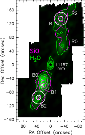
Figure 1: PACS image of L1157 of the integrated H₂O emission at 1669 GHz (from Nisini et al. nisi (2010)). Offsets are with respect to the L1157-mm source, at coordinates $\alpha_{\rm J2000}$ = 20^h 39^m 06$\aas@@fstack{s}$2, $\delta_{\rm J2000}$ = +68$\degr$ 02$\arcmin$ 16$\aas@@fstack{\prime\prime}$0. The contours of the SiO 3-2 integrated intensity is superimposed to the water map with a spatial resolution of 18$\arcsec$ (Bachiller et al. bach01 (2001)). The positions chosen for the HIFI observations (R and B2) are marked by two white circles, which correspond to the largest and the smallest HIFI beam sizes.

However, the red-shifted lobe is more extended than the blue-shifted one and the kinematical ages of the two lobes are found to be the same (15000 yr) indicating that both lobes were created simultaneously. Each outflow lobe shows a clumpy structure and it seems that for each blue clump there is a corresponding red clump symmetrically located with respect to the central source. The symmetry in the individual clumps suggests that the outflow has undergone periods of enhanced ejection and the curved shape suggests that there have been variations in the direction of the driving wind. In addition, the morphology is clearly S-shaped indicating the presence of an underlying precessing jet. The brightest blue-shifted bow-shock, B1, has been imaged at high-angular resolution revealing a clumpy arch-shape structure located at the top of an opened cavity (Tafalla & Bachiller TF95 (1995); Gueth et al. fred98 (1998); Benedettini et al. milena07 (2007); Codella et al. code09 (2009)). L1157-B1 is well traced by species released by dust mantles such as H₂CO, CH₃OH, and NH₃, complex molecules (Arce et al. arce (2008)), and by SiO, which is the standard tracer of high-speed shocks (e.g., Gusdorf et al. gus08b (2008)). In addition, L1157-B1 has been observed with HIFI and PACS spectrometers onboard the Herschel Space Observatory (Codella et al. code10 (2010), Lefloch et al. letter2 (2010)): the preliminary results confirm the rich chemistry associated with the B1 position, also showing bright H₂O emission.

The other bow-shocks have been less studied. As a consequence, it is still unclear how the physical and chemical properties vary along the axis of the L1157 outflow as well as between the blue- and red-shifted lobes.

We present the analysis of various water emission lines observed with HIFI towards two shocked regions in the L1157 outflow, which is observed as part of the the key program WISH (Water In Star-forming-regions with Herschel, van Dishoeck et al. Dish (2011)). The main aim of this paper is to constrain the physical parameters of the gas traced by water lines at the selected B2 and R positions of L1157. We investigate the different excitation conditions of H₂O in this shocked ambient gas in order to compare these conditions with other shock tracers. Since the abundance of water can be strongly affected by shocks, we may thus infer which type of shocks exist in the outflow regions traced by water emission.

2 Observations

Figure 1 presents the PACS map of the water emission at 1669 GHz (from Nisini et al. nisi (2010)). The H₂O map (green contour) is overlaid with contours of the emission from SiO (3-2) (magenta contour) (Bachiller et al. bach01 (2001)) transitions. The water map exhibits several emission peaks corresponding to the positions of previously-known shocked knots, labelled as B0-B1-B2 for the south east blue-shifted lobe, and R0-R-R2 for the north west red-shifted lobe. For our water line observations we selected the shock positions B2 and R because they have different physical and chemical characteristics as shown in many previous works (e.g. Bachiller et al. bach01 (2001)). Observations, from 500 to 1700 GHz, were carried out between May and November 2010 with the use of the HIFI instrument (de Graauw et al. hifi (2010)) in dual-beam switch mode with a nod of 3^′ using fast chopping. The HIFI receivers are double sideband with a sideband ratio close to unity. The data were processed with the ESA-supported package HIPE 5.1 (Herschel Interactive Processing Environment, Ott et al. ott (2010)) for baseline subtraction and then exported after level 2 as FITS files in the CLASS90/GILDAS format. Two polarizations, H and V, were measured simultaneously and then averaged together to improve the signal-to-noise. We checked individual exposures for bad spectra, summed exposures, fitted a low-order polynomial baseline, and integrated line intensities as appropriate. The main beam efficiency ($\eta_{\rm mb}$) depends on frequency and is calculated as described in Roelfsema et al. (Roes (2011)), ranging from to 0.75 to 0.71 in the 535–1670 GHz range. The absolute calibration uncertainty was estimated to be $\sim$10$\%$. At a velocity resolution of 1 km s^-1, the rms noise is 2–20 mK ($T$_A scale) for frequencies less than 1113 GHz and 60 mK at 1669 GHz.

Table 1: List of molecular species and transitions observed with HIFI in L1157 B2 and R. Peak velocity, intensity (in $T$_A scale), integrated intensity (not corrected for beam efficiency, $F_{\rm int}$), minimum and maximum velocities (V_min, V_max), and linewidth (FWHM) are reported.

Transition	$\nu_{\rm 0}$a	$E_{\rm u}$a,b	$HPBW$	$T_{\rm peak}$	rmsc	$V_{\rm peak}$	$V_{\rm max}$	$V_{\rm min}$	$FWHM$	$F_{\rm int}$
	(MHz)	(K)	($\arcsec$)	(mK)	(mK)	(km s-1)	(km s-1)	(km s-1)	(km s-1)	(mK km s-1)
B2 ($\alpha_{\rm J2000}$ = 20h 39m 12$\aas@@fstack{s}$50, $\delta_{\rm J2000}$ = +68$\degr$ 00$\arcmin$ 41$\aas@@fstack{\prime\prime}$0)
o$\--$H218O ($1_{10}$$\--$$1_{01}$)	547676.44	27	38	10.3(2)d	3	+1.8(0.3)d	+7	–4	5.4(0.6)d	59(7)d
o$\--$H2O ($1_{10}$$\--$$1_{01}$)	556936.01	27	38	200(13)e	13	+2.7(1)e	+12	–9	–	8360(40)
p$\--$H2O ($2_{11}$$\--$$2_{02}$)	752033.23	137	28	270(14)d	16	+2.4(0.2)d	+7	–7	4.8(0.2)d	1368(55)d
o$\--$H2O ($3_{12}$$\--$$3_{03}$)	1097364.79	215	19	125(17)d	19	+1.6(0.2)d	+13	–3	4.4(0.4)d	583(61)d
p$\--$H2O ($1_{11}$$\--$$0_{00}$)	1113342.96	53	19	75(20)e	20	+2.6(1.0)e	+12	–9	–	4510(33)
o$\--$H2O ($2_{12}$$\--$$1_{01}$)	1669904.77	80	13	47(60)e	60	+2.6(1.0)e	+11	–11	–	4221(120)
R ($\alpha_{\rm J2000}$ = 20h 39m 01$\aas@@fstack{s}$00, $\delta_{\rm J2000}$ = +68$\degr$ 04$\arcmin$ 31$\aas@@fstack{\prime\prime}$0)
o$\--$H2O ($1_{10}$$\--$$1_{01}$)	556936.01	27	38	256(5)	5	+19.6(1.0)	+35	–3	–	5027(31)
p$\--$H2O ($2_{11}$$\--$$2_{02}$)	752033.23	137	28	176(13)	13	+7.7(1.0)	+30	+7	–	2103(60)
o$\--$H2O ($3_{12}$$\--$$3_{03}$)	1097364.79	215	19	154(22)e	22	+6.4(1.0)e	+21	–2	–	1633(99)
p$\--$H2O ($1_{11}$$\--$$0_{00}$)	1113342.96	53	19	228(15)	15	+19.6(1.0)	+27	–5	–	2555(74)
o$\--$H2O ($2_{12}$$\--$$1_{01}$)	1669904.77	80	13	–	$<$222	–	–	–	–	–

^a Frequencies and spectroscopic parameters have been extracted from the Jet Propulsion Laboratory molecular database (Pickett et al. pickett (1998)).

^b With respect to the ground H₂O level $1_{01}$ for the ortho-H₂O level and $0_{00}$ for the para-H₂O level, respectively.

^c At a spectral resolution of 1 km s^-1.

^dGaussian fit when the observed profile is a gaussian-like.

^eMeasurements taken at the dip of the emission line.

3 Results

A total of 17 emission lines were detected. Table 1 lists the observed H₂O lines, associated with a wide range of excitation energies (27 K$\leq$$E_{\rm u}$$\leq$215 K). In addition, a detection of o$\--$H₂¹⁸O $1_{10}$$\--$$1_{01}$ in B2 will help us to constrain the optical depth. Also, in the observed spectral bands, additional molecular transitions have been detected in the B2 bow-shock, such as NH₃ ($1_{0}$–$0_{0}$), HCO⁺(6–5), CH₃OH–E ($11_{1,10}$–$10_{1,9}$), and C¹⁸O (5–4). On the other hand, the ¹³CO (10–9) line has been observed but not detected (see Table 2).

3.1 Water profiles

The B2 and R water spectra shown in Fig. 2 (here in units of antenna temperature, $T$_A) were smoothed to a velocity resolution of 1 km s^-1, to allow comparisons between all water transitions.

Figure 2: Molecular line profiles observed towards L1157-B2 and R: species and transitions are reported in the panels. The vertical dashed line indicates the ambient LSR velocity (+ 2.6 km s^-1 from C¹⁸O emission; BP97)

The spectra measured in R are consistently fainter than those measured in B2 and the water transition at 1669 GHz appears to be barely detected at R. In the B2 spectra the profiles show a weak red emission and those lines with $E$_u$\leq$80 K show absorption at ambient velocity. The B2 spectra also show bright emission and peaks close to the systemic velocity while the bulk of the R emission is definitely red-shifted. The B2 spectra have a narrower velocity range than those observed at the R position. This could reflect a different shock velocity or simply be a consequence of a different inclination on the plane of sky.

Interestingly, the 557 GHz profile observed at B2 is associated with a much narrower wing (highest blue-shifted velocity, -9 km s^-1) than that observed in B1 (-25 km s${}^{-}1$), studied in the framework of the CHESS GT Key Project (see Fig. 3; Codella et al. code10 (2010), Lefloch et al. letter2 (2010)). This could be an indication of lower shock velocities at B2. On the other hand, B2 has a broader red wing than B1, supporting the idea that the profiles are strongly affected by geometrical effects. Further comparison of H₂O profiles from observations obtained in B1 and B2, would be instructive and will be performed when the full set of CHESS water data will be available.

We note that the profiles in B2 narrow with increasing line excitation, while the line widths (FWZI) in R remain almost constant. In particular, the emission produced by transitions to the ground state level are those that appear broader (see Fig. 2). These spectra are also those affected by the absorption dip and whit a higher $S/N$ level. However, we cannot say if the narrow feature is a real trend.

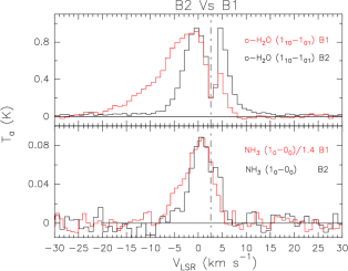
Figure 3: Comparison of water emission lines at 557 GHz and NH₃ ($1_{0}$–$0_{0}$) observed at L1157-B1 (red profiles) and B2 (black profiles). The vertical dashed line indicates the ambient LSR velocity (+ 2.6 km s^-1 from C¹⁸O emission; BP97)

It is also notable that the spectra in R show multiple peaks that present a clear dichotomy with one peak at $\sim$+20 km s^-1 associated with transitions with $E$_u$\leq$60 K and a lower velocity peak at $\sim$+10 km s^-1 associated with transitions with $E$_u$\geq$136 K. Surprisingly the high velocity emission, usually assumed to be emitted from regions close to the fast jet driving the shocks, is associated with the low excitation emission lines. The dichotomy observed in the R bow shock has not been detected in any of the molecules observed so far in L1157. However, as already observed in B2, the difference in the line profiles at various excitation energies could be caused by a large amount of self-absorption in the low velocity range of those lines connecting with the ground state level. In fact, we actually observe a dip in the water emission line at 557 GHz at the systemic velocity. To explain such a striking difference (over 10$\--$20 km s^-1) between the line shapes, as that observed in R, the absorption would have to be caused by outflowing gas. It is evident that further multiline analysis is required to test this assumption. It should also be noted that the same dichotomy has been observed in L1148 at the R4 position by Santangelo et al. (santa (2011)), where they clearly show that this trend is real.

Figure 4 shows the intensity ratio measured towards B2 and R of transitions selected to have different excitation but observed within similar HPBW, in order to minimise effects due to beam dilution. The ratios are plotted only at those velocities at which both lines have $S/N$ $>$3. We note that, besides the obvious effects due to the presence of the absorption dip, the o$\--$H₂O (2₁₂–1₀₁)/p–H₂O (1₁₁–0₀₀) water ratio seems to increase with velocity, while in R it is clear that the p–H₂O (2₁₁–2₀₂)/p–H₂O (1₁₁–0₀₀) water ratio decreases in both the low and high velocity components with respect to the peak at $\sim$8 km s^-1. This effect, with an estimated line ratio error $\leq$30$\%$, reflects the distinctive dichotomy that was observed in the R bow-shock where water transitions with different energy excitations peak at two different velocities.

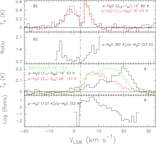
Figure 4: Line temperature water ratios and water profiles in R and B2. Line temperature ratios, as function of velocity, are only shown where the S/N is larger than 3 in both emissions.

In B2, the o–H₂O (1₁₀–1₀₁)/o–H₂¹⁸O (1₁₀–1₀₁) ratio is used to estimate the H₂O optical depth, $\tau_{\rm 16}$, assuming that the two water isotopologues are tracing the same material with the same excitation temperature. To derive the o–H${}_{2}^{16}$O opacity, we need to use the ¹⁶O/¹⁸O ratio for which we take the assumed local ISM value of 560 (Wilson & Rood wilson (1994)). The measured $\tau_{\rm 16}$ value in the low velocity line wings is about 2, which is in agreement with our non-LTE excitation analysis. However, as it cannot be confirmed that the o–H${}_{2}^{16}$O line and the o–H${}_{2}^{18}$O line are associated with the same excitation temperatures, any constraints placed on this value of opacity to infer the column density at B2 would be highly uncertain.

3.2 Other line profiles

Finally, the spectral set-up allowed us to observe also the NH₃ ($1_{0}$–$0_{0}$) fundamental line: a tentative detection (3$\sigma$) of NH₃ is found at R, while relatively bright emission is detected at B2 as found in the nearby blue shock B1 (see Fig 3, Codella et al. code10 (2010)). The ammonia emission, in the L1157 outflow, will be analysed in a forthcoming paper. Table 2 lists the serendipitous detections observed at the B2 bow-shock, HCO⁺ (6$\--$5), CH₃OH-E ($11_{1,10}$$\--$$10_{1,9}$), ¹³CO (10$\--$9) and C¹⁸O (5$\--$4), used to infer the water abundances. The B2 additional spectra are shown in Fig. 5 (here in terms of antenna temperature, $T$_a). Spectra were smoothed to a velocity resolution of 1 km s^-1; they all peak at the systemic velocity and are all associated with a relatively narrow line width ($\leq$ 6 km s^-1) with respect to the water spectra.

Figure 5: Additional emission lines (beside the H₂O and NH₃ profiles reported in Fig. 2) observed at L1157-B2.

Table 2: List of molecular species and transitions observed with HIFI in L1157 B2 and R. Peak velocity, intensity (in $T$_A scale), integrated intensity (not corrected for beam efficiency, $F_{\rm int}$), minimum and maximum velocities (V_min, V_max), and linewidth (FWHM) are reported.

Transition	$\nu_{\rm 0}$a	$E_{\rm u}$a	$HPBW$	$T_{\rm peak}$	rmsb	$V_{\rm peak}$	$V_{\rm max}$	$V_{\rm min}$	$FWHM$	$F_{\rm int}$
	(MHz)	(K)	($\arcsec$)	(mK)	(mK)	(km s-1)	(km s-1)	(km s-1)	(km s-1)	(mK km s-1)
Bow-shock B2
HCO+ (6$\--$5)	535061.40	90	37	19(2)c	3	+2.2(0.1)c	+7	–2	3.3(0.3)c	67(6)c
CH3OH-E ($11_{1,10}$$\--$$10_{1,9}$)	536191.07	169	37	10(2)c	3	+1.6(0.3)c	+7	–4	4.3(0.7)c	48(6)c
C18O (5$\--$4)	548830.97	79	37	24.3(2)c	3	+2.4(0.1)c	+5	–0	2.5(0.3)c	66(3)c
NH3 ($1_{0}$$\--$$0_{0}$)	572498.07	28	38	83.6(8)	8	+0.9(0.2)b	+7	–6	6.2(0.4)b	549(31)c
13CO (10$\--$9)	1101349.65	291	21	–	20	–	–	–	–	–
Bow-shock R
NH3 ($1_{0}$$\--$$0_{0}$)	572498.07	28	38	28(8)	8	+6.6(1.0)	+9	–0	–	105(9)

^a Frequencies and spectroscopic parameters have been extracted from the Jet Propulsion Laboratory molecular database (Pickett et al. pickett (1998)).

^b At a spectral resolution of 1 km s^-1.

^cGaussian fit when the observed profile is a gaussian-like.

4 Excitation Analysis

We ran the RADEX non-LTE model (van der Tak et al. van (2007)) with collisional rate coefficients by Faure et al. (rates (2007)) using the escape probability method for a plane parallel geometry in order to constrain the physical parameters ($T$_kin, $N$${}_{\rm H_{2}O}$ and $n$${}_{\rm H_{2}}$) of water emission. An ortho/para=3 ratio was assumed, equal to the high temperature equilibrium value. To place some constraints on the unknown size of the emitting region, we assumed three different sizes (3$\arcsec$, 15$\arcsec$ and 30$\arcsec$). RADEX does not take into account the near-IR pumping of the H₂O lines where the radiation field is relatively strong and has some impact on the excitation conditions of the emitting gas. However, since both B2 and R position are relatively far from the central source, we expect no continuum to affect our results.

4.1 L1157 B2

At B2, given the presence of the absorption dip and the relatively narrow velocity range, we model the physical parameters of water emission by integrating the H₂O intensity over the whole spectral profile (i.e. neglecting the absorption dip). We will consider the measurements of water transitions with an absorption dip as upper limits. In Fig. 6 we overplot non-LTE RADEX model predictions against integrated flux water ratios. For this analysis, we conservatively assumed an uncertainty of 20$\%$. Coloured triangles with uncertainties are the observed values corrected for beam filling and assuming three different sizes as mentioned in the insert of the plots. The top panel of Fig. 6 shows a plot of the o$\--$H₂O ($3_{12}$$\--$$3_{03}$)/p$\--$H₂O ($1_{11}$$\--$$0_{00}$) ratio versus o$\--$H₂O ($3_{12}$$\--$$3_{03}$), the middle panel shows a plot of the o$\--$H₂O ($2_{12}$$\--$$1_{01}$)/o$\--$H₂O ($1_{10}$$\--$$1_{01}$) ratio versus o$\--$H₂O ($2_{12}$$\--$$1_{01}$), while the bottom panel shows a plot of the o$\--$H₂O ($3_{12}$$\--$$3_{03}$)/o$\--$H₂O ($2_{12}$$\--$$1_{01}$) versus o$\--$H₂O ($3_{12}$$\--$$3_{03}$)/o$\--$H₂O ($1_{10}$$\--$$1_{01}$) ratios.

Some general conclusions can be drawn from the inspection of Fig. 6. The observations are consistent with model predictions only assuming an emission size $>$3$\arcsec$ (black triangle). In particular, a size closer to 15$\arcsec$–30$\arcsec$ in agreement with the L1157 map of the o$\--$H₂O ($2_{12}$$\--$$1_{01}$) line published by Nisini et al. (nisi (2010)) is suggested (see bottom panel). The observed water ratio appears to be well constrained from low values of column density N${}_{\rm H_{2}O}$ $\leq$5x10¹³ cm^-2 (see the top panel), while a density range of 10⁵$\leq$n${}_{\rm H_{2}}$$\leq$10⁷ cm^-3, and temperatures T_kin$\geq$300 K are inferred from all panels. However, because of the presence of the absorption dip in both water transitions plotted in the middle panel, the inferred physical conditions can be only considered as upper limit. In fact, the absorption dip could affect our analysis, which would shift observations towards lower excitation conditions.

With regards to the absorption dip observed in the water ground state transition, if we assume that the absorption is due to foreground gas unrelated to L1157-B2, we estimate, from the standard radiative transfer equation, a 8 K$\leq$$T$_ex$\leq$13 K adopting a 0.1$\leq$$\tau_{16}$$\leq$10. This low value of $T$_ex usually implies low densities or low kinetic temperatures. No other constraints can be inferred due to the uncertainties in the measurements and too many free parameters to fit simultaneously with the RADEX code.

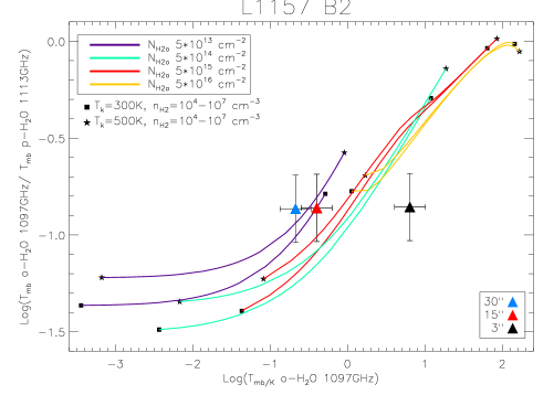
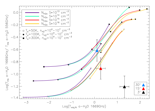
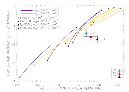
Figure 6: Analysis of the water line emissions in L1157 B2. o$\--$H₂O ($3_{12}$$\--$$3_{03}$)/p$\--$H₂O ($1_{11}$$\--$$0_{00}$) ratio versus o$\--$H₂O ($3_{12}$$\--$$3_{03}$) (in logarithmic scale, top panel), o$\--$H₂O ($2_{12}$$\--$$1_{01}$)/o$\--$H₂O ($1_{10}$$\--$$1_{01}$) ratio versus o$\--$H₂O ($2_{12}$$\--$$1_{01}$) (middle panel), and o$\--$H₂O ($3_{12}$$\--$$3_{03}$)/o$\--$H₂O ($1_{10}$$\--$$1_{01}$) versus o$\--$H₂O ($3_{12}$$\--$$3_{03}$)/o$\--$H₂O ($2_{12}$$\--$$1_{01}$) ratios (bottom panel), for non-LTE (RADEX) plane parallel models at the labelled temperatures. A linewidth of 5.5 km s^-1 has been assumed, according to the observed spectra. Each coloured curve corresponds to the labelled $N$${}_{\rm H_{2}O}$ (see insert at the top-left corner). H₂ density increases from left to right as the labelled values. Triangles with error bars indicate the size of the emitting region (30$\arcsec$, 15$\arcsec$, 3$\arcsec$).

4.2 L1157 R

In the water profiles of the bow-shock R, Fig. 2 shows an evident dichotomy at different excitations where two emission peaks at different velocities clearly displaying different excitation conditions. Thus, we modelled the emission by splitting the lines into two components (hereafter called LV, at $\sim$+10 km s^-1, and HV, at $\sim$+20 km s^-1). In Fig. 7 we overplotted non-LTE RADEX model predictions against the observed LV and HV $T$_mb water ratios. The top panel of Fig. 7 shows a plot of the o$\--$H₂O ($3_{12}$$\--$$3_{03}$)/o$\--$H₂O ($1_{10}$$\--$$1_{01}$) ratio versus o$\--$H₂O ($3_{12}$$\--$$3_{03}$), while the bottom panel of Fig 7 shows a plot of the p$\--$H₂O ($1_{11}$$\--$$0_{00}$)/o$\--$H₂O ($3_{12}$$\--$$3_{03}$) ratio versus p$\--$H₂O ($1_{11}$$\--$$0_{00}$).

A first conclusion that can be drawn is that the LV component appears to be associated with higher excitation conditions than the HV component and we can exclude a point-like source (i.e. the 3$\arcsec$ case) based on the inconsistency of column density, which can be derived from the two panels. For the low excitation HV, we have standard kinetic temperatures $\geq$100 K and a degeneracy between column density and hydrogen density: either N${}_{\rm H_{2}O}$$\sim$5x10¹³ cm^-2 and n${}_{\rm H_{2}}$$\sim$10⁶ cm^-3 or N${}_{\rm H_{2}O}$$\sim$5x10¹² cm^-2 and n${}_{\rm H_{2}}$$\sim$10⁷ cm^-3. On the other hand, for the high excitation LV emission the observed water ratio traces temperatures T_kin$\geq$300 K, as well as surprisingly dense gas with n${}_{\rm H_{2}}$$\sim$10⁸ cm^-3 and low column density, N${}_{\rm H_{2}O}$$<$5$\times$10¹³ cm^-2. The tentative detection of NH₃ ($1_{0}$$\--$$0_{0}$) emission at these velocities seems to support a very high density solution.

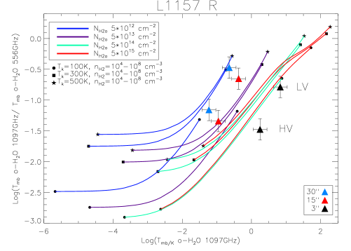
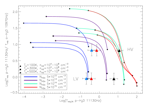
Figure 7: Analysis of the water line emission in L1157 R. o$\--$H₂O ($3_{12}$$\--$$3_{03}$)/o$\--$H₂O ($1_{10}$$\--$$1_{01}$) ratio versus o$\--$H₂O ($3_{12}$$\--$$3_{03}$) (in logarithmic scale, top panel), and p$\--$H₂O ($1_{11}$$\--$$0_{00}$)/o$\--$H₂O ($3_{12}$$\--$$3_{03}$) ratio versus p$\--$H₂O ($1_{11}$$\--$$0_{00}$) (bottom panel), for non-LTE (RADEX) plane parallel models at the labelled temperatures. A linewidth of 10 km s^-1 has been assumed, consistent with the observed spectra. Each coloured curve corresponds to the labelled $N$${}_{\rm H_{2}O}$ (see insert). H₂ density increases from left to right as the labelled values. Triangles with error bars indicate the size of the emitting region (30$\arcsec$, 15$\arcsec$, 3$\arcsec$).

5 On the origin of water emission in L1157

In summary, Table  3 outlines the physical conditions traced by water that we constrain from our analysis.

Table 3: Physical conditions traced by water lines.

B2	R-LV	R-HV
Tkin$\geq$300 K	Tkin$\geq$300 K	Tkin$\geq$100 K
105$\leq$n${}_{\rm H_{2}}$$\leq$ 107 cm-3	n${}_{\rm H_{2}}$ $\sim$ 108 cm-3	N${}_{\rm H_{2}O}$ $\sim$5x1013 cm-2, n${}_{\rm H_{2}}$$\sim$106 cm-3
N${}_{\rm H_{2}O}$$\leq$5x1013 cm-2	N${}_{\rm H_{2}O}$$<$5x1013 cm-2	N${}_{\rm H_{2}O}$ $\sim$5x1012 cm-2, n${}_{\rm H_{2}}$$\sim$107 cm-3
Inferred size 15$\arcsec$–30$\arcsec$	Inferred size $>$3$\arcsec$	Inferred size $\geq$15$\arcsec$

The water at B2 traces lower density environments than that at R-LV and R-HV. In addition, the main difference between R-LV and R-HV is that H₂O at R-HV traces lower temperatures and densities with respect to R-LV. The physical parameters derived in B2 and R-HV are in reasonable agreement with those measured by Nisini et al. (nisi7 (2007)), using multi transitions observations of a classical jet tracer like SiO. On the other hand, the density inferred for R-LV (n${}_{\rm H_{2}}$$\sim$10⁸ cm^-3) is higher with respect to that derived from SiO emission by two orders of magnitude. Actually, the SiO profiles as observed at the R position (see Fig. 4) cast serious doubts on the theory that emission from these species has a common physical origin. In addition, our results strongly support the conclusion of Nisini et al. (nisi (2010)) that water emission seems to follow quite closely the distribution of H₂ emission. In fact, the general physical conditions inferred in the R bow shock (T_kin$\geq$300 K, n${}_{\rm H_{2}}$$\sim$10⁶–10⁷ cm^-3) are consistent with those derived for the H₂ in Nisini et al. (nisiApj (2010)).

5.1 Water abundances

We derive, at the R bow shock position, the H₂O abundance, with respect to H₂, using the $N$(H₂) estimated by Nisini et al. (nisi7 (2007)) and in B2 using the C¹⁸O (5-4) line emission detected in the present survey (see Fig. 5 and Tab. 2). The velocity averaged H₂O abundance for R is $\sim$10^-6–10^-7.
The H₂O abundance for B2 is estimated to be $\sim$10^-6 assuming [C¹⁸O]/[H₂]=2$\times$10^-7 (Wilson $\&$ Rood wilson (1994)) in the temperature range from 300 to 500 K (see Table  3). This result is consistent with the water abundance found at B1 at low velocities (Lefloch et al. letter2 (2010)). On the other hand, the X(H₂O) measured at the highest velocities in B1 is 2 orders of magnitude greater than in B2 ($\sim$10^-4). These differences could provide evidence for an older shock in B2 compared to the one in B1.
The results found in R are comparable with those obtained by Santangelo et al. (santa (2011)) in the L1448 outflow. These low water abundances could support the possibility of having a J-shock instead of a C-shock where the H₂O abundance is expected to be $\sim$10^-4 relative to H₂. Alternatively, the low water abundances measured could also be evidence of either an old shock where the water in the gas phase has had time to be depleted on grains or of UV dissociation of H₂O (see Bergin et al. bergi98 (1998)).

5.2 Comparison with shocks models

Theoretical studies indicated that, under typical interstellar conditions, shocks faster than $\sim$20 km s^-1 are efficient enough to free much of the water ice frozen on grain surfaces (Draine et al. Draine (1983)), while shocks faster than $\sim$15 km s^-1, through gas-phase chemical reactions, produce large quantities of water (Kaufman & Neufeld Kau (1996)). After the shocked gas has cooled enhanced water abundances of $\sim$10^-4 relative to H₂ can endure for as long as 10⁵ yr (Bergin et al. bergi98 (1998)). Sub-millimeter and far-infrared water emission lines are very efficient coolers, therefore large interstellar water abundances produced by the shock processing are relevant for the thermal evolution of the gas (e.g., Neufeld et al. neu95 (1995)). Observations of a number of excited molecular transitions in L1157 clearly indicate that shocks are present in both lobes. The present dataset deserves a more detailed comparison with shock models. In this present paper we only discuss our data using models provided by literature.

We have compared a grid of C- and J-type shocks spanning different velocities (10 to 40 km s^-1) and two pre-shock densities (2$\times$10⁴ and 2$\times$10⁵ cm^-3) provided by Flower $\&$ Pineau des For$\hat{\rm e}$ts (fiore10 (2010)), with the observed intensities. Figure 8 shows the observed line ratios with respect to the high energy ($E$_u=215 K) 1097 GHz line for different sizes of B2, R-LV and R-HV against the predicted shock line ratios. From our analysis, none of these models seem to be able to properly reproduce the absolute intensities of the water emissions observed.

Particularly in the case of the R-HV component, a degeneracy is noticeable because, for an emitting region of size 30$\arcsec$, both a speed of 10 km s^-1 with a pre-shock density of 2$\times$10⁵ cm^-3 and a speed of 30 km s^-1 with a pre-shock density of 2$\times$10⁴ cm^-3 can be inferred for both types of shock. This is consistent with the analysis made in the water diagnostic plots (Fig. 7). The same sort of degeneracy can be drawn for the R-LV component, where we do not find a satisfactory solution that matches the full sample of water transitions. The most plausible explanation is given by, in agreement with Fig. 7, a size of 3$\arcsec$ for a C-type shock with a speed of 30 km s^-1 and pre-shock density of 2$\times$10⁴ cm^-3, and for a J-type shock with a speed of 20 km s^-1 and pre-shock density of 2$\times$10⁵ cm^-3.

Regarding the B2 position, a lower speed of J-shocks around 10 km s^-1 is inferred. Two different solutions are found: (i) a pre-shock density of 2$\times$10⁴ and 3$\arcsec$ of size, or (ii) a pre-shock density of 2$\times$10⁵ and 15$\arcsec$ of size. According to our previous water analysis an emitting size of 15$\arcsec$ looks more plausible. These preliminary results call for detailed modelling for a more complete analysis. Note, for instance, that UV H₂O dissociation is not taken into account in the grid of shock models used.

C-shocks have been recently invoked by Flower $\&$ Pineau des For$\hat{\rm e}$ts (fiore10 (2010)) and Viti et al. (viti (2011)) modelling L1157 B1. On the other hand, recent results obtained with PACS in the course of the CHESS spectral survey key-program (Benedettini et al. in prep.) required J-shocks to explain the CO excitation conditions in L1157 B1. This scenario could also provide a possible explanation of our analysis in B2 and R where both C- and J -type shocks seem to be required.

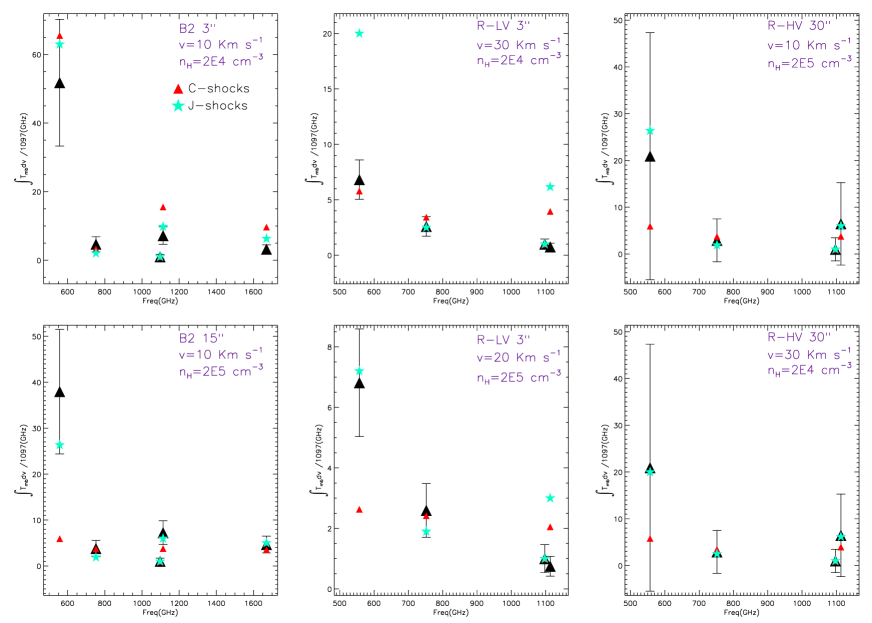
Figure 8: Comparison between the observed HIFI H₂O line ratios of the two velocity components in R and B2 for different sizes (black triangles) and those predicted by C-type (red triangle) and J-type (cyan triangles) shock models from Flower $\&$ Pineau des For$\hat{\rm e}$ts (fiore10 (2010)).

6 Conclusions

We have presented a water emission observed in the 500–1700 GHz band towards the two bow-shocks B2 and R, of the L1157 proto-stellar outflow. The main conclusions are the following:

1. The comparison between H₂O and SiO profiles, and their physical characteristics casts serious doubt on the assumption that emission from these species has a similar physical origin.

2. We derive H₂O abundances for R $\sim$10^-6–10^-7 and for B2 $\sim$10^-6. This result is consistent with the water abundance found at B1 at low velocities. On the other hand, the X(H₂O) measured at the highest velocities in B1 is 2 orders of magnitude greater than in B2 ($\sim$10^-4). These differences could provide evidence for an older shock in B2 compared to that in B1.

3. The emerging scenario highlights the importance of J-shocks, expected to be associated with a thin layer and very densely compressed material in these environments. The results found in R are comparable with those obtained by Santangelo et al. (submitted) in the L1448 outflow. These low water abundances could support the possibility of having a J-shock instead of a C-shock.

4. Interestingly, the highest excitation conditions are observed at low velocities. However, if we assume that high excitation is tracing portions of gas near the shock, we could solve this apparent contradiction by assuming that we are observing a very collimated region located along the plane of the sky. In this case the fast collimated gas should be reprojected and thus have lower radial velocities. On the other hand, a less excited region could be more extended, which would result in a wider velocity range due to the geometry.

- (1) Arce H.G, Santiago-García J., Jørgensen J. K., et al. ApJ 681, L21-L24
- (2) Bachiller R., & Peréz Gutiérrez M., 1997, ApJ 487, L93 (BP97)
- (3) Bachiller R., Peréz Gutiérrez M., Kumar M. S. N., et al. 2001, A&A 372, 899
- (4) Benedettini M., Viti S., Codella C., et al. 2007, MNRAS 381, 1127
- (5) Bergin, E. A., Neufeld, D. A., & Melnick, G. J., 1998, ApJ, 499, 777
- (6) Bjerkeli, P., Liseau, R., Olberg, M., et al. 2009, A&A, 507, 1455
- (7) Codella C., Benedettini M., Beltrán M. T., et al. 2009, A&A 507, L25
- (8) Codella C., Lefloch B., et al. 2010, A&A 518, L112
- (9) de Graauw Th., Helmich F.P., Phillips T. G., et al. 2010, A&A 518, L6
- (10) Draine, B. T., Roberge, W. G., & Dalgarno, A. 1983, ApJ, 264, 485
- (11) Faure, A., Crimier, N., Ceccarelli, C., et al. 2007, A&A, 472, 1029
- (12) Flower, D. R., & Pineau des Forts, G., 2010, MNRAS, 406, 1745
- (13) Franklin, J., Snell, R. L., Kaufman, M. J., et al. 2008, ApJ, 674, 1015
- (14) Gueth F., Guilloteau S., & Bachiller R., 1998, A&A 333, 287
- (15) Gusdorf A., Cabrit S., Flower D., et al. 2008, A&A, 482, 809
- (16) Kaufman, M. J., & Neufeld, D. A. 1996, ApJ, 456, 611
- (17) Kristensen, L.E., Visser, R., van Dishoeck, E.F. et al. 2010, A&A, 521, L30
- (18) Lefloch B., Cabrit S., Codella C., et al. 2010, A&A 518, L113
- (19) Liseau et al. 1996, A&A, 315, 181
- (20) Neufeld D.A., & Green S., 1994, ApJ 432, 158
- (21) Neufeld, D. A., Lepp, S., & Melnick, G. J. 1995, ApJS, 100, 132
- (22) Nisini B., Codella C., Giannini T., et al. 2007, A&A, 462, 163
- (23) Nisini B., Benedettini M., Codella C., et al. 2010, A&A, 518, L12
- (24) Nisini, B., Giannini, T., Neufeld, D. A., et al. 2010b, ApJ, 724, 69
- (25) Ott, S. 2010, in Astronomical Data Analysis Software and Systems XIX, ed. Y. Mizumoto, K.-I. Morita, & M. Ohishi, ASP Conf. Ser.
- (26) Pickett H. M., Poynter R.L., Cohen E. A., et al. 1998, JQSRT, 60, 883
- (27) Roelfsema, P. R., Helmich, F.P., Teyssier D., et al. 2011, A&A, submitted
- (28) Santangelo, G., Nisini, B., Giannini, T., et al. 2011, A&A, in press
- (29) Tafalla M., & Bachiller R., 1995, ApJ, 443, L37
- (30) Zhang Q., Ho P. T. P. & Wright M. C. H., 2000, ApJ, 119, 1345
- (31) van Dishoeck, E. F., Kristensen, L. E., Benz, A. O., et al. 2011, PASP, 123, 138
- (32) van der Tak F. F. S., Black, J. H., Schøier F. L., et al. 2007, A&A, 468, 627
- (33) Viti, S., Jimenez-Serra, I., Yates, J. A., Codella C., et al. 2011, ApJ, 740, L3
- (34) Wilson, T. L., & Rood, R. T., 1994, ARA&A, 32, 191