Heat exchanges in coarsening systems

Abstract

This paper is a contribution to the understanding of the thermal properties of aging systems where statistically independent degrees of freedom with largely separated timescales are expected to coexist. Focusing on the prototypical case of quenched ferromagnets, where fast and slow modes can be respectively associated to fluctuations in the bulk of the coarsening domains and to their interfaces, we perform a set of numerical experiments specifically designed to compute the heat exchanges between different degrees of freedom. Our studies promote a scenario with fast modes acting as an equilibrium reservoir to which interfaces may release heat through a mechanism that allows fast and slow degrees to maintain their statistical properties independent.

PACS:

I Introduction

When two equilibrium systems in contact with reservoirs at different temperatures $T_{1}$ and $T_{2}$ are put in contact, heat flows from the hotter to the colder and the usual equilibrium concept of temperature can be used to establish the average direction of heat fluxes. Deviations from the average are described by a fluctuation principle known as the Gallavotti-Cohen relation GC , namely

$$\ln\frac{P(Q_{1,2})}{P(-Q_{1,2})}=Q_{1,2}\left(\frac{1}{T_{2}}-\frac{1}{T_{1}}\right),$$ (1)

where $P(Q_{1,2})$ is the probability that the first system exchanges the heat $Q_{1,2}$ in a certain (sufficiently long) time with the other one and we have set to unity the Boltzmann constant.

In an attempt to generalize ideas of equilibrium thermodynamics to non-equilibrium systems, an effective temperature $T_{eff}$ has been introduced in 7dipeliti in the context of non-equilibrium stationary systems and in 89dipeliti for aging systems. In this formulation, $T_{eff}$ can be evinced from the relation

$$R(t,t_{w})=T_{eff}(t,t_{w})^{-1}\frac{\partial C(t,t_{w})}{\partial t_{w}}$$ (2)

between the auto-correlation function $C(t,t_{w})=\langle O(t)O(t_{w})\rangle-\langle O(t)\rangle\langle O(t_{w})\rangle$ of the observable $O$ at times $t$ and $t_{w}<t$ and the associated linear response function, $R(t,t_{w})=\lim_{h\to 0}\delta O(t)/\delta h(t_{w})$, where $h$ is a small perturbation introducing an extra term $-h(t)O$ in the Hamiltonian. In equilibrium states, due to the fluctuation-dissipation theorem, $T_{eff}=T$ is the usual temperature which is independent of the two times and on the chosen observable $O$. Out of equilibrium, in principle $T_{eff}$ may depend on $t,t_{w}$ and $O$ and is not necessarily related to the temperature of the reservoir. In peliti it was argued that $T_{eff}$ exhibits the properties of a temperature, in the sense that it regulates the direction of heat fluxes favouring thermalization. Specifically, if different degrees of freedom effectively interact on a given time scale, heat flows from those with higher $T_{eff}$ to those with a lower one. The concept of effective temperature is possibly relevant when thermal flows are small; in the context of aging systems this usually amounts to consider the large time regime. Generally, in this asymptotic domain one can identify fast and slow degrees of freedom whose typical timescales $t_{f}$ and $t_{s}$ become widely separated. Indeed, while $t_{f}$ is generally age-independent, $t_{s}$ is usually an increasing function of the age $t_{w}$ of the sample. When this happens, one can probe fast or slow degrees increasing the times $t,t_{w}$ along particular directions in the $t,t_{w}$ plane. Specifically, by letting $t_{w}\to\infty$ keeping $t-t_{w}$ finite, since $t-t_{w}\ll t_{s}$ the slow degrees act adiabatically and can be considered as static. In this time sector, denoted as the short time difference (or quasi-equilibrium) regime, one probes the dynamical behavior of fast modes. Conversely, letting again $t_{w}\to\infty$ but keeping $t/t_{w}$ (or some different combination of $t$ and $t_{w}$ in specific systems) finite one has $t-t_{w}\sim t_{w}\sim t_{s}$, focusing the analysis on the timescale of the slow (or aging) components. In this time sector, usually denoted as aging regime, the fast degrees act as a stationary background and the time evolution of the slow modes is probed. In a class of aging systems, among which mean field p-spin models and coarsening systems parisi , the effective temperature (here and in the following we simply quote the name for the quantity $T_{eff}$ defined through Eq. (2), without necessarily conforming to the debated interpretation of it as a thermodynamic temperature) takes two different well defined values in the short time and in the aging regime. In the former sector one has $T_{eff}=T$, the bath temperature, while in the aging regime $T_{eff}=T_{s}>T$. A major difference between mean field glassy models and phase-ordering systems is that $T_{s}$ is finite in the former, while it is infinite in the latter. This simple two-temperature scenario, as opposed to that of a continuously varying $T_{eff}$ displayed by models with full replica symmetry breaking, such as the Sherrington-Kirkpatrik spin glass, or some systems without local detailed balance detbal , is amenable of a simple interpretation in terms of fast and slow components: The former which are already at the equilibrium temperature and the latter retaining a self-generated higher temperature $T_{s}$. Generally, the existence of different effective temperatures in the asymptotic domain implies that thermalization among different degrees of freedom is suppressed. While on the whole the mechanism whereby thermalization is avoided is uncertain, in the case of coarsening systems, at least in the solvable large-$N$ model ($N$ being the number of components of the vector order parameter) fast and slow degrees can be explicitly exhibited and their statistical independence can be proved noilargen . This is consistent with two temperatures being sustained and coexist in the system. However, the issue of heat exchanges occurring between fast and slow modes has never carefully been analyzed so far.

In this paper we tackle this question numerically in the physical case of coarsening systems with $N=1$. We check to some extent the picture with slow and fast degrees, studying the heat exchanges between them, and suggesting a mechanism whereby statistical independence is preserved and effective thermalization does not occur. In particular, we will consider the two-dimensional Ising model quenched below $T_{c}$. This is perhaps the simplest case where the two-degrees/two-temperature scenario can be investigated. We mention that the Ising model in $d=1$ exhibits an anomalous coarsening behavior with a continuously varying $T_{eff}$ lippiello which, moreover, is found to depend on the particular observables $O$ entering $R$ and $C$ in the definition. These features, which are presumably related to the fact that the model is at the lower critical dimensionality $d_{L}$ claudio , make the interpretation of $T_{eff}$ as a genuine temperature doubtful. However, for $d>d_{L}$ these features disappear and the two-temperature scenario is more sound.

The paper is organized in five sections. In Sec. II we review the kinetics of binary systems in contact with a single thermal bath. In Sec. III we consider a system in contact with two reservoirs and introduce the method to compute heat exchanges. In Sec. IV we describe our numerical experiments to study heat flows in phase-ordering systems. In Sec. V we draw the conclusions and discuss the perspective of this work.

II Dynamics of binary systems in contact with a single heat bath

The dynamics of a non-disordered binary system (i.e. one that can be described by the ferromagnetic Ising model) in contact with a thermal bath, has been extensively studied since a long time. Although exact results are scarce, the overall phenomenology is nowadays quite well understood bray . Hereafter we recall some basic facts that will be needed in the following and specify our dynamical model, that will be later (in Sec. III) generalized to the case of a system in contact with two reservoirs.

In the high temperature disordered phase, for $T>T_{c}$, the system is ergodic and equilibrium is achieved on microscopic timescales (if not too close to $T_{c}$) starting from any configuration. On the other hand, the evolution below $T_{c}$ depends strongly on the initial state. In particular, if the sample is prepared in a broken symmetry configuration (for instance, with all spins up) the dynamics converges on a microscopic time to the broken symmetry equilibrium state. This is characterized by finite coherence length $\xi$ and relaxation time $t_{eq}\propto\xi^{z}_{eq}$, where $z_{eq}$ is the usual equilibrium dynamical exponent. $\xi$ and $t_{eq}$ can be interpreted as the spatial extent and the persistence of thermal islands of reversed spins in the sea of opposite magnetization. These fluctuations will be denoted as fast, because $t_{eq}$ is finite (and small if $T$ is sufficiently far from $T_{c}$). Conversely, starting from a typical high temperature equilibrium configuration, namely a disordered one, and quenching to a sub-critical temperature, a coarsening dynamics sets in where domains of the two magnetized phases with a typical size $L(t)$ grow in time. For the case of a dynamics with non-conserved order parameter considered in this paper one has $L(t)\propto t^{1/z}$, with $z=2$, for sufficiently long times. If an interface is present at time $t_{w}$ in some part of the system, it must move a distance of order $L(t_{w})$ in order to produce an effective decorrelation. Since this takes a time of order $t_{s}\propto L(t_{w})^{z}\propto t_{w}$, the characteristic decorrelation time due to interface motion is $t_{s}\propto t_{w}$. This is the essence of the aging phenomenon, where the evolution gets slower as time elapses and $t_{s}$ diverges. The interfacial degrees of freedom responsible for the aging process will be denoted as slow. However, these are not the only degrees contributing to the dynamics. Indeed, the interior of domains is basically in equilibrium in one of the broken symmetry phases described above. It is then characterized by the fast thermal fluctuations with characteristic timescale $t_{f}=t_{eq}$. In conclusion, in the late stage evolution of a coarsening system there are two dynamical components, fast and slow, whose timescales are widely separated in the large $t_{w}$ limit.

In this paper we will consider the two-dimensional Ising model, where $N$ discrete spin variables $\sigma_{i}=\pm 1$ defined on the sites $i$ of a square lattice are governed by the Hamiltonian $H(\sigma)=-J\sum_{\langle i,j\rangle}\sigma_{i}\sigma_{j}$. Here $\sigma$ denotes the whole spin configuration and the sum is running over all nearest neighbours couples $\langle i,j\rangle$. The critical temperature of the model is $T_{c}=2J[atanh(1/\sqrt{2})]^{-1}\simeq 2.269\,J$. In the following we will set $J=1$.

We introduce a dynamics where a single spin update is attempted in each timestep; time will be measured in Montecarlo steps (or sweeps), corresponding to $N$ timesteps. Metropolis single spin transition rates

$$w(\sigma)=min\left[\exp\left(\frac{-\delta E}{T}\right),1\right],$$ (3)

where $\delta E$ is the energy change due to the flip, will be used.

In order to study the evolution, let us consider the energy (per spin) $E(t)=(1/N)\langle H(t)\rangle$ whose equilibrium value is $E_{eq}$. Here $\langle\ldots\rangle$ means an average over thermal noise and initial conditions. Since the excess energy $\Delta E(t)=E(t)-E_{eq}$ is associated to the domain boundaries, in the coarsening stage one has

$$\Delta E(t)\propto L(t)^{-1}\propto t^{-1/2}.$$ (4)

This behavior lasts until $L(t)$ becomes comparable with the size of the system and the system either equilibrates or remains trapped (particularly at low temperatures) in long lived metastable states with one (or few) spanning interfaces. If the thermodynamic limit is taken from the beginning the system is free from finite size effects and coarsening lasts forever: Equilibration is then never observed.

Snapshots of the configurations of the system after a quench from a disordered state to a subcritical temperature $T<T_{c}$ are shown in Fig. (1), where the growing domains are visible. One can also see small regions of reversed spins inside the growing domains. These are the fast degrees of freedom, with the equilibrium behavior discussed above.

In Fig. (2) the time behavior of the excess energy $\Delta E$ is shown. In the case of a quench to $T=0$, after an initial transient, it starts decreasing with the expected power-law behavior up to a certain time where finite-size effects set in and saturation occurs. Increasing $N$ the finite-size effect is delayed, as expected. The same behaviour is observed in a quench to $T>0$, the main difference being a value of $z$ slightly larger than the expected one $z=2$ due to preasymptotic corrections, as discussed in isingt0 .

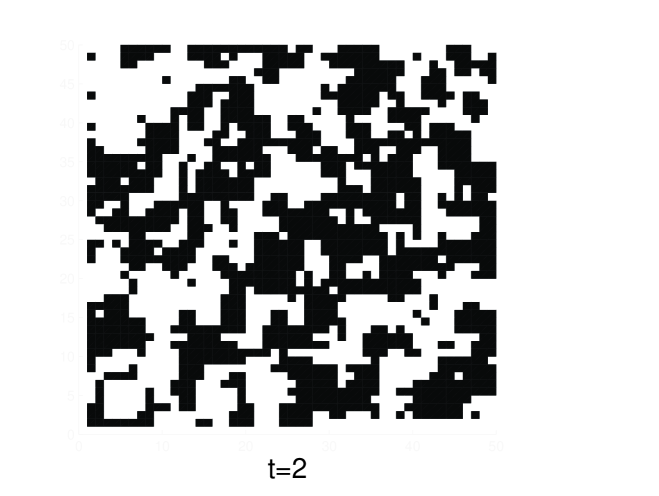
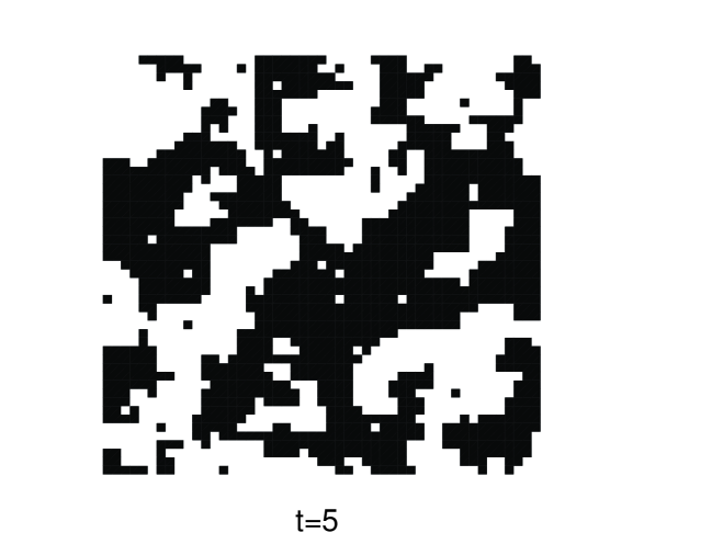
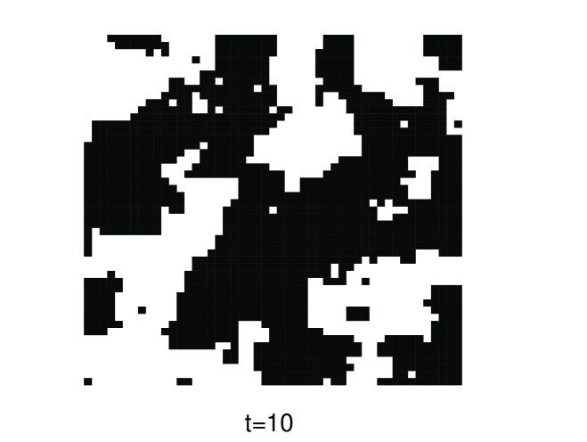
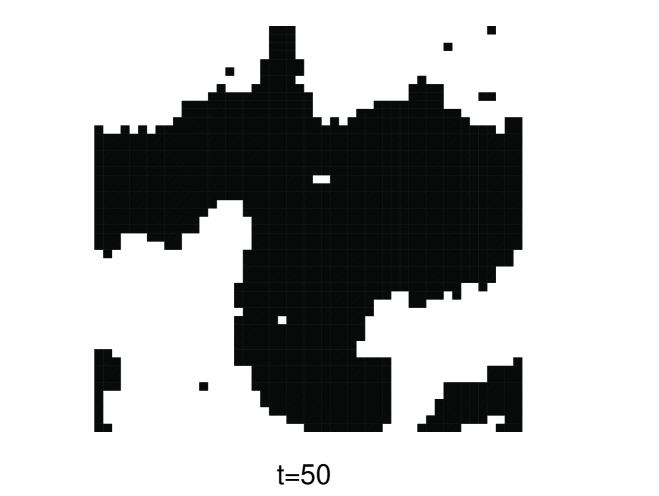
Figure 1: (Color online). Domain configurations at different times $t$ after a quench to $T=1.5$. Black and white regions correspond to up and down spins. The system size is $N=50$x$50$.

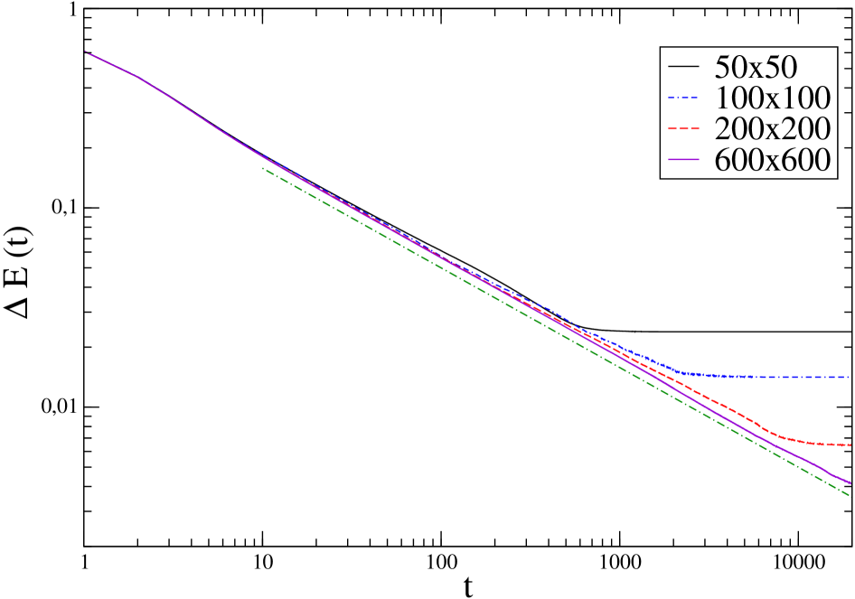
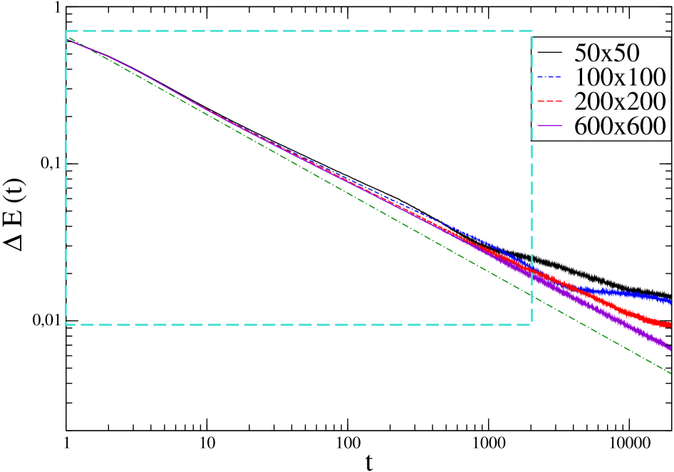
Figure 2: (Color online). The behavior of the excess energy $\Delta E(t)$ after a quench to $T=0$ (left panel) and to $T=1.5$ (right panel) is shown for different system sizes (see key). Averages are taken over $10^{3}$ realizations. The dashed line is the power law behavior $\Delta E\propto t^{-1/2}$ expected in the scaling regime. The area in the box corresponds to the time region where heat exchanges are computed (see Sec. (I)).

III The Ising model in contact with two heat baths

We consider now the case of two coupled binary systems (denoted simply as 1 and 2) interacting with thermostats $T_{1}$ and $T_{2}$ at different temperatures $T_{1}>T_{2}$ (for simplicity we use the same symbols for the temperature of the reservoirs and the reservoirs themselves). We denote with $Q_{T_{1},1}$ ($Q_{T_{2},2}$) the heat flowing in a time interval $I_{\tau}=[t_{w},t_{w}+\tau]$ from the system 1 (2) to the thermostat $T_{1}$ ($T_{2}$ ), and with $Q_{1,2}$ that passing from 1 to 2.

When $T_{1},T_{2}>T_{c}$, starting from any initial condition, the system attains a non-equilibrium stationary state after a certain (microscopic) time. The same behavior is observed if one (or both) the temperatures are below $T_{c}$, provided that the system(s) coupled to a sub-critical temperature is prepared in an initial state with broken symmetry, in order to avoid the coarsening dynamics. The statistics of the heats exchanged between the systems and the thermostats has been investigated analytically by a mean field approach in meanf and numerically in noi . The case where one or both the systems are interested by phase-ordering kinetics has not been studied yet, and will be considered in Sec. IV. This case poses the problem of a direct measurement of $Q_{1,2}$, as it is discussed below.

In general the heat exchanged between two parts of a system or between a part of a system and a thermostat in the time interval $I_{\tau}$ can be written as

$$Q=\sum_{s=t_{w}}^{t_{w}+\tau}\,\,\sum_{i=1}^{n(s)}q_{i}(s)$$ (5)

where $q_{i}(s)$ is the heat exchanged by a single degree (a spin, in the Ising model) in an unit time around time $s$ and $n(s)$ is the number of degrees of freedom which can effectively exchange the heat. Eq. (5) can be straightforwardly used for the computation of the heats $Q_{T_{1},1}$, $Q_{T_{2},2}$. In a numerical simulation the $q_{i}(s)$ are the energies $\delta E$ released by the thermostats in the flip of the $i-th$ spin (according to Eq. (3)) in the Montecarlo step occurring at time $s$.

When the system is stationary, a direct computation of $Q_{1,2}$ can be avoided because for $\tau$ large enough its value can be related to $Q_{T_{1},1}$ and $Q_{T_{2},2}$. Indeed, denoting with $\delta E_{1}^{(\tau)}$ the energy stored in the system 1 (and analogously for 2) in the time interval $I_{\tau}$ ($\delta E_{1}^{(\tau)}=E_{1}(t_{w}+\tau)-E_{1}(t_{w})$), one has $\delta E_{1}^{(\tau)}=Q_{T_{1},1}-Q_{1,2}$ and $\delta E_{2}^{(\tau)}=Q_{T_{2},2}+Q_{1,2}$. Combining these equations one has

$$Q_{1,2}=\frac{1}{2}\left[Q_{T_{1},1}-Q_{T_{2},2}\right]+\frac{1}{2}\left[\delta E_{2}^{(\tau)}-\delta E_{1}^{(\tau)}\right].$$ (6)

In a stationary state the quantities $n(t)$ and $q_{i}(t)$ of Eq. (5) fluctuate around a $t$-independent average value. Hence $\langle Q_{T_{1},1}\rangle$ and $\langle Q_{T_{2},2}\rangle$ grow proportionally to $\tau$. On the other hand the boundary term $\delta E_{2}^{(\tau)}-\delta E_{1}^{(\tau)}$ is finite (for a finite system). Hence, in the large-$\tau$ limit one can compute $Q_{1,2}$ as

$$Q_{1,2}\simeq\frac{1}{2}\left[Q_{T_{1},1}-Q_{T_{2},2}\right].$$ (7)

Therefore, in this case, it is sufficient to collect the statistics of the heats $Q_{T_{1},1}$ and $Q_{T_{2},2}$ exchanged with the thermostats and, from this, the distribution of $Q_{1,2}$ can be determined through Eq. (7), and Eq. (1) can be tested. This was made in noi with a numerical setup where a two-dimensional Ising model on a $L$ x $L$ square lattice was divided into two interacting halves of size $L/2$ x $L$ (system 1 and 2), in contact with the two heat baths.

In Sec. IV we will prepare the two systems as containing fast modes (system 1) and a mixture of fast and slow ones (system 2). Heat fluxes between different degrees will then be inferred from the knowledge of $Q_{1,2}$. However, in this case, since 2 is aging, it is no longer true that $n(t)$ and $q_{i}(t)$ fluctuate around time-independent values and, hence, Eq. (7) cannot be used. For this reason we need another operative definition of the quantity $Q_{1,2}$. This is the subject of the remaining of this section. In order to do that, it is first useful to understand the basic mechanisms whereby heat is transferred at stationarity. This can be better illustrated by considering first the case of two systems made by one single spin each. We also assume, for the moment, that the two spins are updated alternately with Metropolis transition rates. Denoting with $1_{\uparrow}$ and $1_{\downarrow}$ the two possible states of system 1 (and similarly for 2), let us consider the case of an initial state $1_{\uparrow},2_{\uparrow}$ which evolves in four steps as follows

$$1_{\uparrow},2_{\uparrow}\quad\Rightarrow\quad 1_{\downarrow},2_{\uparrow}\quad\Rightarrow\quad 1_{\downarrow},2_{\downarrow}\quad\Rightarrow\quad 1_{\uparrow},2_{\downarrow}\quad\Rightarrow\quad 1_{\uparrow},2_{\uparrow}$$ (8)

eventually returning to the initial state. In the initial state the system is in the lowest energy state. Since 1 is in contact with the higher temperature bath, it has a larger probability to be flipped first. If this happens, as in the first step in the scheme (8), the heat $Q_{T_{1},1}=2$ (equal to the energy increase $\delta E$ of the system) is transferred from the reservoir $T_{1}$ to 1. Now it is the turn of 2 to be updated. With Metropolis rates it flips with probability one, because in doing so the energy decreases. Then the heat $Q_{T_{2},2}=2$ is released by 2 to $T_{2}$ (step two). At this stage a heat $Q=2$ has been transferred between $T_{1}$ and $T_{2}$: Hence we conclude that the amount $Q_{1,2}=Q$ has flown between the two spins. Now the system is again in the lowest energy state and, as before, the most probable evolution is the reversal of 1, where a heat $Q_{T_{1},1}=2$ is again taken from the reservoir (step three). This move surely induces the flip of 2 (step four) with a heat $Q_{T_{2},2}=-2$ flowing to $T_{2}$ and another amount $Q_{1,2}=Q$ exchanged between the two systems. In conclusion, if this process happens, a heat $Q_{1,2}=4$ flows from 1 to 2. Clearly, one can analogously imagine a process where $Q_{1,2}=-4$, but this process implies that 2 flips first, which is less probable. This explains why, on average, $Q_{1,2}$ is positive, even if negative fluctuations (which in stationary states are regulated by Eq. (1)) are possible. The physical mechanism described above is such that heat is transferred from one system to the other whenever the flip of one spin triggers the flip of the other. It is then quite natural to introduce a direct measure of the heat flow as $Q_{1,2}(\tau)=\sum_{s=t_{w}}^{t_{w}+\tau}\delta E(s)\sum_{j}\epsilon_{j}\delta_{s,s^{trig}_{j}}$, where $\delta E(s)$ is the energy variation of the system in the $s$-th step belonging to the interval $I_{\tau}$, $s^{trig}_{j}$ is a subset of steps where a flip has been triggered by a previous reversal of the other spin, and $\epsilon_{j}=\pm 1$ depending on the direction of the heat flow. We state that the flip of (say) 2 in the $s_{j}$-th step has been triggered if 1 and 2 were not aligned before reversing 2, and 1 was the last spin flipped before $s_{j}$. In this case heat is flowing from 1 to 2 and hence $\epsilon_{j}=1$. In the opposite situation in which 1 is flipping at time $s_{j}$ and 2 was flipped previously one has $\epsilon_{j}=-1$.

The same definition is meaningful if a different sequence of updates (i.e. random) is assumed and/or different transition rates are considered (i.e. Glauber). The main difference in this case is that after the flip of 1, spin 2 is not forced to flip and it might happen that 1 recovers again its original value. However in this case there is no heat transfer between 1 and 2, and this process does not alter the computation of $Q_{1,2}$.

Let us now consider the case of systems with many degrees of freedom. The mechanism described in (8) is at work between any couple of spins on the interface between 1 and 2. Clearly, many other processes, involving also other spins away from the interface, may occur. However, they do not overrule our algorithm, since there is no heat transfer between 1 and 2 until the process arrives on the boundary between them. Therefore, we can adopt the same operative definition for the heat transferred between any couple of spins on the interface, and $Q_{1,2}$ is then obtained by summing all these contributions.

In order to test this method, we have prepared a system with the geometry discussed below Eq. (7) in a stationary state, and we have computed $Q_{1,2}$ with this technique and, independently, $Q_{T_{1},1}$ and $Q_{T_{2},2}$. If the method is reliable, the determination of $Q_{1,2}$ should verify Eq. (7) for large $\tau$, so the probability distributions $P_{a}(Q)=P(Q_{1,2}=Q)$ and $P_{s}(Q)=P([Q_{T_{1},1}-Q_{T_{2},2})/2]=Q)$ should obey $P_{a}(Q)=P_{s}(Q)$. These distributions are compared in Fig. 3. For small $\tau$ they are quite different. This is expected due to the presence of the boundary term in Eq. (6). Increasing $\tau$, however, the boundary term becomes comparably smaller and the two curves tend to merge. To be more quantitative we plot, in the inset of Fig. 3, the distance

$$d_{as}=\sqrt{\int_{-\infty}^{\infty}[P_{a}(Q)-P_{s}(Q)]^{2}dQ}$$ (9)

between the two probability densities, showing that it is a steadily decreasing function. This shows that the algorithm for the direct measurement of $Q_{1,2}$ is reliable. When one (or both) of the systems is aging, Eq. (7) is spoiled by the extra heat released to the baths because the system is lowering its energy due to relaxation. In these cases the direct computation of $Q_{1,2}$ according to the technique described above is mandatory. In the following, it will always be used to compute $Q_{1,2}$.

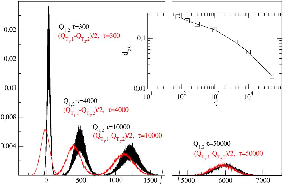
Figure 3: (Color online).Comparison between $P[(Q_{T_{1},1}-Q_{T_{2},2})/2]$ and $P(Q_{1,2})$ computed in a system of size $L=50$ in a stationary state with $T_{1}=2$ and $T_{2}=1.5$, for different values of $\tau$, as specified in the plot. The statistics is collected over $1.7\times 10^{6}$ realizations. In the inset the distance $d_{as}$ between the two distributions is plotted.

IV Heat exchanges in phase-ordering

In this section we study the heat exchanges in phase-ordering systems. We do this with the help of some numerical experiments designed to collect the statistics of the heat flowing between fast and slow degrees and among them and the reservoir. This will allow us to test the scenario with two statistically independent degrees coexisting at different (effective) temperatures and to discuss why such independence may be retained in the evolution.

In order to do that, the straightforward procedure would be to consider an aging system, to recognize and discriminate (at any time) fast and slow components, and hence to detect the heat they are exchanging. However, this is not easily realizable. Indeed, although in a coarsening system we have an idea of what slow and fast modes are, a precise definition and separation of degrees is to a large extent arbitrary. Moreover, if even one could find a technique suited to do that, this would be tuned to phase-ordering and the method would be restricted to coarsening systems. Instead, we propose a different approach where two systems are coupled. Preparing such systems so that the first is in equilibrium while the second coarsens, as will be detailed below, one may assume that slow degrees are confined in the second. As we shall discuss, this will allow us to proceed to the discussion of heat exchanges. In doing that, we adopt the same geometry as for the stationary case described in the previous section except that, in order to guarantee that the heat exchanged is small enough we have activated only two links, at distance $L/2$, between the two systems. In all the cases we have chosen the parameters in such a way that the system is free from finite-size effects. System 1 is prepared in equilibrium at the temperature $T_{1}$ while system 2 is in an infinite temperature disordered configuration. At time $t=0$, sample 2 is brought in contact with the thermostat at the temperature $T_{2}<T_{c}$ while 1 interacts with a bath at the same temperature $T_{1}$ of its initial equilibrium state. Then, from time $t$ onwards 2 ages via phase-ordering kinetics, while 1 remains in a stationary configuration. Precisely, 1 is not stationary in principle, due to the coupling with the non-stationary system 2, but this effect is negligible for large system sizes and few active links between the two sub-systems. Moreover the effect is further suppressed in the asymptotic time domain, due to the progressive decrease of the number of slow degrees in sample 2. Indeed our simulations did not show any deviation from stationarity in 1. The statistics of the heats is collected from some time $t_{w}$ to $t_{w}+\tau$ in a sample of size $L=100$. Notice that in the range of times considered in this simulation, represented by the dashed box in the right panel of Fig. 2, finite-size effects can be neglected.

Indicating with $F_{1}$, $F_{2}$ the fast degrees of freedom of the two coupled systems, with $S_{2}$ the slow ones, and with $Q_{F_{1},F_{2}}$ the heat exchanged between $F_{1}$ and $F_{2}$ (and similarly for the heat exchanged between fast and slow ones), the general scheme of all the possible heat exchanges is summarized in figure 4.

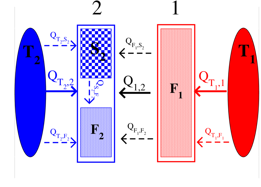
Figure 4: (Color online). Schematic description of the system according to the two-degrees scenario. Systems 1 and 2 are represented as blue and red boxes, and are in contact with the reservoirs $T_{1}$ and $T_{2}$, represented as ellipses. The heat exchanged between the two systems ($Q_{1,2}$), and between the systems and the respective reservoirs ($Q_{T_{1},1}$ and $Q_{T_{2},2}$) are represented as bold arrows (heats flowing in the direction of the arrows are considered positive). Fast and slow degrees are represented as separate subsystems by the boxes $F_{1}$, $F_{2}$ and $S_{2}$. All the possible heat exchanges among them and between them and the reservoirs are indicated with dashed arrows.

We start with the case in which the two baths are at the same temperature $T_{1}=T_{2}=1.5$. This will allow us to draw some conclusion on the possibility that, in a single coarsening system, heat is released directly from the slow modes to the fast ones. The probability distributions of $Q_{T_{1},1}$, $Q_{T_{2},2}$ and of $Q_{1,2}$ have been computed letting $x=\tau/t_{w}$ fixed while $t_{w}$ is increased (we used values of $t_{w}$ up to $t_{w}=1000$, for different choices of $x$). This will be referred to as the aging limit. For every choice of $t_{w}$ and $x$ we found a pattern of behaviors analogous to the one shown in Fig. 5, where $t_{w}=80$ and $x=1$. Here one sees that $\langle Q_{T_{2},2}\rangle<0$, because 2 is transferring the excess energy associated to the interfaces to the bath $T_{2}$. On the other hand the heat $\langle Q_{1,2}\rangle$ is very small. This happens because with the present geometry $Q_{1,2}$ can be exchanged only through two links and because we are working in the aging limit. Indeed, while $F_{1}$ and $F_{2}$ are equilibrated at the same temperature, and hence $\langle Q_{F_{1},F_{2}}\rangle=0$, $\langle Q_{F_{1},S_{2}}\rangle<0$ is the only contribution to $\langle Q_{1,2}\rangle$. However, in the aging limit since $\tau\propto t_{w}$ and the number of slow modes which contribute to $\langle Q_{1,2}\rangle$ is $\langle n(t_{w})\rangle\propto t_{w}^{-1/2}$, there is a number of order $t_{w}^{1/2}$ of terms in the double sum in Eq. (5). On the other hand, for the heats exchanged involving only fast degrees, such as $\langle Q_{F_{1},F_{2}}\rangle$, $\langle Q_{F_{1},T_{1}}\rangle$, and $\langle Q_{F_{2},T_{2}}\rangle$, $n(t_{w})$ is constant and hence there is a number of order $t_{w}$ of terms contributing in Eq. (5). Therefore, the heat $\langle Q_{1,2}\rangle$ is negligible with respect to the others. This shows that our experiments are performed in the limit of small average heat exchanged between the two systems. However, although small, $\langle Q_{1,2}\rangle$ is not strictly zero and its behavior parallels that of $Q_{T_{2},2}$. This can be seen in Fig. 6 where $\langle Q_{1,2}\rangle$, $\langle Q_{T_{2},2}\rangle$ and their ratio is plotted for different choices of $x$. In the inset of this figure one sees that, after an initial transient, $\langle Q_{T_{2},2}\rangle$ decays as $t_{w}^{-1/2}$. A similar behavior is found for $\langle Q_{1,2}\rangle$, the main difference being an oscillating behavior superimposed on the $t_{w}^{-1/2}$ decay. The origin of such oscillations is not completely clear and is probably related to the recurrent passage of interfaces across the boundary links. Their amplitude can be suppressed by increasing $x$, because collecting the heats on larger time windows effectively averages out the oscillating behavior. For $x\gtrsim 50$ the periodic behavior is basically washed away. Notice also that the curves tend to superimpose as $x$ increases. The ratio $\langle Q_{1,2}\rangle/\langle Q_{T_{2},2}\rangle$ is plotted in the main part of the figure, showing that for sufficiently large values of $t_{w}$ and $x$ it converges to a constant value, namely $\langle Q_{1,2}\rangle$ and $\langle Q_{T_{2},2}\rangle$ are proportional. This behavior supports the hypothesis that slow degrees transfer heat to the fast ones and to the reservoir basically in the same way. This is so because, since fast degrees are thermalized with the reservoirs they affect the slow ones similarly to what the thermal baths do, namely absorbing heat.

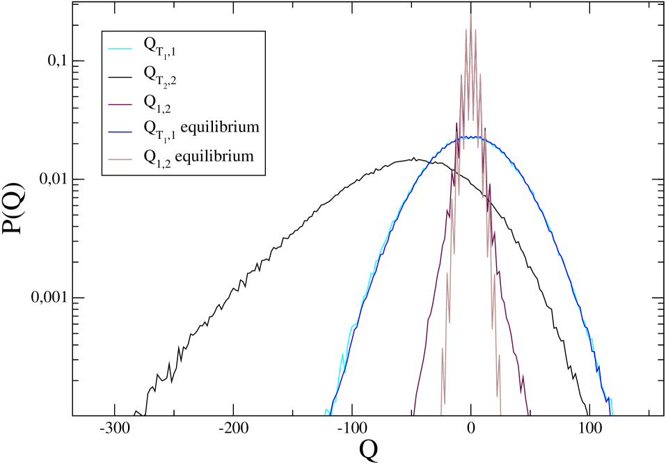
Figure 5: (color online). $P(Q_{T_{1},1})$, $P(Q_{T_{2},2})$ and $P(Q_{1,2})$ for an aging system coupled to a (quasi) stationary one in contact with baths at the same temperatures $T_{1}=T_{2}=1.5$, with $t_{w}=80$ and $x=\tau/t_{w}=1$. The distributions $P(Q_{T_{1},1})$ and $P(Q_{1,2})$ of the case where both sub-systems are in equilibrium at the same temperature $T_{1}=T_{2}=1.5$ are also shown. The statistics is collected over $2\times 10^{5}$ realizations.

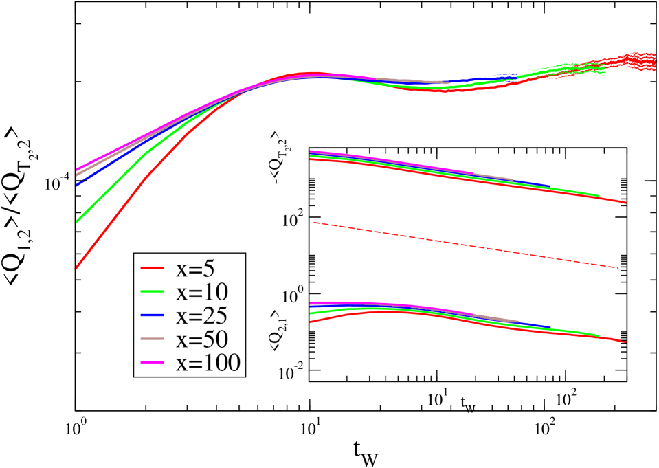
Figure 6: (color online). The ratio $\langle Q_{1,2}\rangle/\langle Q_{T_{2},2}\rangle$ is plotted against $t_{w}$ for different values of $x$ (see key). Data are averaged over $3.6\times 10^{7}$ realizations. The clouds around the bold curves represent the error bars. In the inset $\langle Q_{1,2}\rangle$ and $\langle Q_{T_{2},2}\rangle$ are plotted separately. The dashed line is the power law $t_{w}^{-1/2}$.

Let us see how these findings fit into the scenario with two degrees coexisting at different (effective) temperatures. This framework implies that statistical independence is retained and thermalization does not occur between them. The question is why. The most obvious explanation would be that slow and fast degrees do not effectively interact; they are insulated, in some sense. However, the above experiment has shown that this is not the case, since heat is transferred from slow degrees to the fast ones and to the reservoir basically in the same way. Hence, statistical independence must have a different origin. A possible explanation is the following: Let us consider two separated domains at time $t_{1}$ (left part of Fig. (7)). They successively merge at the later time $t_{2}>t_{1}$, releasing some heat $Q$ to the fast degrees surrounding the coalescence event. This excess heat will outflow to the bath on the microscopic time $t_{eq}$. After the event the slow degrees which have originally released the heat are annihilated. The surviving ones are left unmodified by this process, and hence retain their original properties. In summary, if energy release is always accompanied by annihilation, the heat transferred between fast and slow components up to a certain time was provided by interfaces that do not exist any more, while those still surviving have never been involved. Notice that, writing $\Delta E(t)=\Delta E(t_{w})+Q(\tau)$, where $Q(\tau)$ is the heat released to the reservoir, from Eq. (4) one has $Q(\tau)\propto n_{s}(t)-n_{s}(t_{w})$, where $n_{s}$ is the number of slow degrees. This shows that $Q(\tau)$ is proportional to the decrease of $n_{s}$, and this is consistent with the hypotheses that heat release and annihilation are deeply related processes.

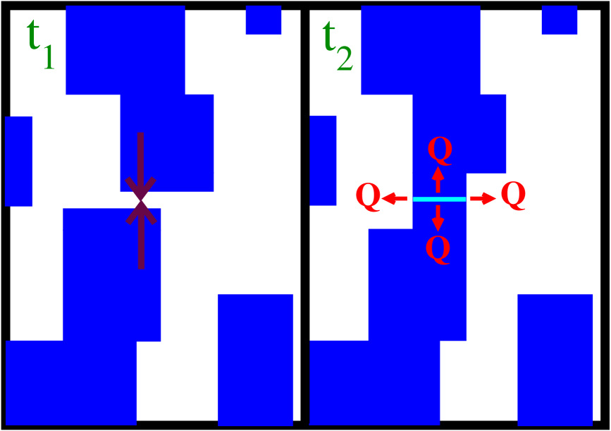
Figure 7: (Color online). Schematic description of the process of interface annihilation and subsequent heat release to the fast degrees.

Having shown that fast degrees absorb the excess heat released by the interfaces it remains to be shown that this process does not spoil the thermal properties of the fast degrees, preserving in this way the statistical independence. This is expected because bulk degrees are able to thermalize among themselves and with the reservoirs in a microscopic time $t_{eq}\ll t_{s}$, making their thermal properties irrespective of the presence of interfaces. If this is true, one might predict that when two coarsening systems quenched to different temperatures $T_{1}$, $T_{2}<T_{1}$ are put in contact, heat flows from the fast components of the hotter system to those of the colder. Moreover, fluctuations of heat exchanged between fast modes should be similar to those observed in stationary systems and, in particular, governed by the fluctuation principle (1). Strictly speaking, we should verify Eq. (1) but with $Q_{F_{1},F_{2}}$ in place of $Q_{1,2}$. However, we recall that Eq. (1) is supposed to hold in the large-$\tau$ domain where boundary terms can be neglected, similarly to what happens in Eq. (6). In this regime the number of bulk spins is much larger than that of the interfacial ones and so $Q_{F_{1},S_{2}}$ is negligible with respect to $Q_{F_{1},F_{2}}$. Then, if the thermal properties of fast degrees is unaffected by the presence of the slow ones one should be able to verify the FR (1) for the whole heat transferred $Q_{1,2}$.

In order to study this, we have designed an experiment similar to the one discussed above. However now we quench system 1 to $T=T_{1}=2<T_{c}$, while 2 is in equilibrium at $T_{2}=1.5$. In Fig. 8 we compare the probability distribution $P_{a}(Q_{1,2})$ of the heat $Q_{1,2}$ in this experiment, with the one $P_{s}(Q_{1,2})$ measured in the experiment described in Sec. (III) where the samples are again in contact with the same baths at $T_{1}=2,T_{2}=1.5$, but they are both stationary. The two distributions have a zig-zag shape. This is not due to a lack of statistics but is a genuine feature that we will discuss later. Notice that, at any finite time, the positive tail of $P_{a}(Q_{1,2})$ is fatter than that of $P_{s}(Q_{1,2})$. This is due to the extra heat flowing from the coarsening system 1 to the stationary sample 2, which is produced by the reduction of the interface density, similarly to the case with $T_{1}=T_{2}$ discussed above (see Fig. 5). Besides this, one observes that the two distributions tend to merge in the large time limit when all boundary terms become negligible and slow degrees are sufficiently few. We made this observation more quantitative by plotting, in one inset of Fig. 5, the distance $d_{as}$ between the two probability densities, defined in Eq. (9), which decreases in a power-law way. The merging of the two distributions indicates that the thermal properties of the fast degrees are left unchanged by the presence of the slow ones. As a further check we consider the validity of Eq. (1): After having verified that the l.h.s. of Eq. (1) is well fitted by $\ln[P(Q_{1,2})/P(-Q_{1,2})]=k(\tau)(1/T_{2}-1/T_{1})Q_{1,2}$ for all the values of $\tau$, we have plotted the slope $k(\tau)$ in the inset of the bottom-right panel of Fig. 8. One sees that $k(\tau)$ converges to $k(\tau)=1$ when $\tau$ is increased, as expected.

Let us now come back to the zig-zag feature of the distributions of Fig. 8. which can be explained as follows. Let us consider the 4-steps microscopic heat transfer process (8). According to our operative definition of $Q_{1,2}$, one measures $Q_{1,2}=2$ or $Q_{1,2}=4$ after the first or after the fourth step, respectively. This implies that $Q_{1,2}$ is always a multiple of 2, in this model. In the situations considered in this Section spin 2 is part of an extended system in contact with the reservoir at $T_{2}<T_{c}$. This system is in a coarsening stage, where the up-down symmetry is not globally broken. However locally, the neighborhood of spin 2 has almost surely a broken symmetry character, if time is large enough. Indeed, this spin will almost surely be located in the bulk of a magnetized domain. Suppose that symmetry is broken around the $\uparrow$ direction. In this situation the probability of finding the first or the last configuration of the process (8) is much higher than that of finding the other. Since the final time $t=t_{w}+\tau$ over which the heats are collected is not correlated to the spin configurations, one has a much higher probability that $Q_{1,2}$ is a multiple of 4 than that it is not. This explains the zig-zag behavior where values of $Q_{1,2}$ which are multiples of 4 are enhanced.

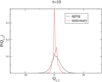
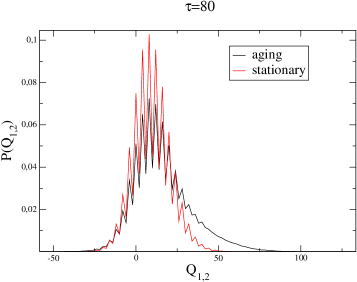
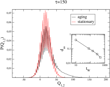
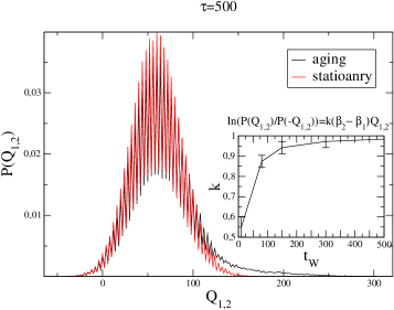
Figure 8: (Color online). Comparison between $P(Q_{1,2})$ computed in a stationary state with $T_{1}=2$, $T_{2}=1.5$ and in the setup where 2 is (quasi)-stationary at $T_{2}=1.5$ while 1 is aging after a quench to $T_{1}=2$. The system size is $L=50$. Different values of $\tau$ are shown, with $x=\tau/t_{w}=1$. The statistics is collected over $10^{6}$ realizations. In the inset of the left-bottom panel the distance $d_{as}$ is plotted against $t_{w}$. In the inset of the right-bottom panel the values of the slope $k$ obtained from the fluctuation-relation (see text) are plotted against $t_{w}$.

V Conclusions and perspectives

Coarsening systems are prototypical models which exhibit a non trivial aging behavior where two classes of degrees of freedom with different properties can be identified and studied to some extent. They are then particularly suited to understand the issue of thermal exchanges in aging states and the related concept of effective temperatures. In this perspective, in this paper we have studied numerically the heat flows occurring in an Ising model quenched below the critical temperature. In order to do that we have first developed an algorithm to quantify the heat transferred between two parts of a system, and we have subsequently used this tool in a series of numerical experiments designed as to detect the heat fluxes occurring between the two kinds of degrees existing in the coarsening system. Our results fit into a scenario where fast components thermalize with the reservoirs and act themselves as baths where interfaces can temporary store their excess energy when annihilation events occur. The mechanism is such that, after a microscopic time of order $t_{eq}$, the statistical properties of both fast and slow modes are left unchanged. This guarantees that the two kind of degrees may remain statistically independent, as shown analytically in a soluble limit in noilargen . Once a thermodynamic interpretation of the effective temperature (in the spirit of Ref. peliti ) is agreed upon (let us mention however that our results do not speak about the consistent interpretation of $T_{eff}$ as a genuine thermodynamic temperature) our results help to explain why a couple of different effective temperature can be sustained indefinitely. At variance to what is naively expected, this does not occur because the two classes of degrees are thermally insulated, or not effectively interacting. On the contrary, heat is exchanged between them much in the same way as it is exchanged with the baths. The mechanism whereby this occurs, nevertheless, is such to preserve the statistical properties of the two kind of modes. We have given support to this allegation by proving that the Gallavotti-Cohen FR (1) is obeyed in the asymptotic domain also when aging occurs in systems at different temperatures. Let us stress here that $T_{1}$ and $T_{2}$ entering Eq. (1) are in this case the temperatures of the thermal baths. The presence of $T_{eff}$ does not play an appreciable role in our experiments because slow degrees do not contribute significantly to the heat exchanged $Q_{1,2}$, which is dominated by the contribution of the fast spins. Interestingly, $T_{eff}$ might be expected to enter the FR cugzam if only the heat exchanged by slow degrees was considered, (namely subtracting away the dominant contribution provided by the fast ones in a specially designed experiment).

Acknowledgements.

F.C. acknowledges financial support from PRIN 2007JHLPEZ (Statistical Physics of Strongly correlated systems in Equilibrium and out of Equilibrium: Exact Results and Field Theory methods).

References

- (1) D.J. Evans , E.G.D. Cohen and G.P. Morriss G P, Phys. Rev. Lett. 71, 2401 (1993). D.J. Evans and D.J. Searles, Phys. Rev. E 50, 1645 (1994). G. Gallavotti and E.G.D. Cohen, J. Stat. Phys. 80, 931 (1995). Phys. Rev. Lett. 74, 2694 (1995).
- (2) P. C. Hohenberg and B. I. Shraiman, Physica D 37, 109 (1989). M. C. Cross and P. C. Hohenberg, Rev. Mod. Phys. 65, 851 (1993). M. S. Bourzutschky and M. C. Cross, Chaos 2, 173 (1992). M. Caponeri and S. Ciliberto, Physica D 58, 365 (1992).
- (3) L. F. Cugliandolo and J. Kurchan, Phys. Rev. Lett. 71, 173 (1993); Phil. Magaz. B 71, 50 (1995); J. Phys. A 27, 5749 (1994).
- (4) L. F. Cugliandolo, J. Kurchan, and L. Peliti, Phys. Rev. E 55, 3898 (1997).
- (5) G.Parisi, F.Ricci-Terzenghi and J.J.Ruiz-Lorenzo, Eur.Phys.J. B 11, (1999) 317.
- (6) F. Corberi, G. Gonnella, E. Lippiello, and M. Zannetti, Europhys. Lett. 60, 425 (2002); J. Phys. A 36, 4729 (2003). N. Andrenacci, F. Corberi, and E. Lippiello, Phys. Rev. E 73 046124 (2006).
- (7) F. Corberi, E. Lippiello, and M. Zannetti Phys. Rev. E 65, 046136 (2002).
- (8) C. Godrèche and J.M. Luck, J.Phys. A 33, 1151 (2000). E. Lippiello and M. Zannetti, Phys.Rev.E 61, 3369 (2000). F. Corberi, E. Lippiello, and M. Zannetti, Phys. Rev. E 63, 061506 (2001); Eur. Phys. J. B 24, 359 (2001); Jstat, P12007 (2004). F. Corberi, A. de Candia, E. Lippiello, and M. Zannetti, Phys. Rev. E 65, 046114 (2002).
- (9) F. Corberi, E. Lippiello, and M. Zannetti, J. Stat. Mech. P12007 (2004). F. Corberi, C. Castellano, E. Lippiello, and M. Zannetti, Phys. Rev. E 70, 017103 (2004). F. Corberi, C. Castellano, E. Lippiello, and M. Zannetti, Phys. Rev. E 65, 066114 (2002).
- (10) A.J. Bray, Adv. Phys. 43, 357 (1994).
- (11) G. Manoy and P. Ray, Phys. Rev. E 62, 7755 (2000). E. Lippiello, F. Corberi, and M. Zannetti, Phys.Rev.E 74, 041113 (2006). F.Corberi, E.Lippiello, and M.Zannetti, Phys.Rev.E 78, 011109 (2008).
- (12) V. Lecomte, Z. Racz, and F. van Wijland, J. Stat. Mech. P02008 (2005).
- (13) A. Piscitelli, F. Corberi, and G. Gonnella, J. Phys. A: Math. Theor. 41 332003 (2008). A. Piscitelli, F. Corberi, G. Gonnella, and A. Pelizzola, J. Stat. Mech. P01053 (2009).
- (14) M. Sellitto, cond-mat/9809186. F.Zamponi, F.Bonetto, L.F.Cugliandolo, and J.Kurchan, J.Stat.Mech. P09013 (2005). M. Sellitto, Phys. Rev. E 80, 011134 (2009).