Global GRMHD Simulations of Black Hole Accretion Flows: a Convergence Study

Abstract

Global, general relativistic magnetohydrodynamic (GRMHD) simulations of nonradiative, magnetized disks are widely used to model accreting black holes. We have performed a convergence study of GRMHD models computed with HARM3D. The models span a factor of $4$ in linear resolution, from $96\times 96\times 64$ to $384\times 384\times 256$. We consider three diagnostics of convergence: (1) dimensionless shell-averaged quantities such as plasma $\beta$; (2) the azimuthal correlation length of fluid variables; and (3) synthetic spectra of the source including synchrotron emission, absorption, and Compton scattering. Shell-averaged temperature is, except for the lowest resolution run, nearly independent of resolution; shell-averaged plasma $\beta$ decreases steadily with resolution but shows signs of convergence. The azimuthal correlation lengths of density, internal energy, and temperature decrease steadily with resolution but show signs of convergence. In contrast, the azimuthal correlation length of magnetic field decreases nearly linearly with grid size. We argue by analogy with local models, however, that convergence should be achieved with another factor of $2$ in resolution. Synthetic spectra are, except for the lowest resolution run, nearly independent of resolution. The convergence behavior is consistent with that of higher physical resolution local model (“shearing box”) calculations and with the recent nonrelativistic global convergence studies of Hawley et al. (2011).

1 Introduction

The numerical study of black hole accretion flows has advanced significantly in the last decade. The advent of techniques for numerically solving the equations of general relativistic magnetohydrodynamics (GRMHD) has enabled self-consistent global modeling of accretion driven by the magneto-rotational instability (MRI) (Balbus & Hawley, 1991; Gammie, 2004) onto rotating black holes. Qualitative aspects of these simulations are code independent (e.g. De Villiers & Hawley, 2003; Gammie et al., 2003; Anninos et al., 2005), but quantitative variations raise the question of numerical convergence. Recent work has shifted focus from dynamical properties of the accretion flow to simulated observations that can potentially constrain parameters for particular sources such as Sgr A* (Dolence et al., 2009; Moscibrodzka et al., 2010; Dexter et al., 2009, 2010), including polarized radiative transfer (Shcherbakov et al., 2010). To assess the credibility of these radiative models, it is necessary to assess quantitative convergence of the underlying GRMHD simulations.

Convergence studies of global accretion models are computationally expensive. An alternative is to use a local model with shearing box boundary conditions to study the dynamics of MRI driven turbulence. These are simpler in the sense that there are fewer free parameters, and cheaper in that numerical resolution can be focused on a few correlation volumes $\sim H^{3}$, where $H$ is the disk scale height. The local model has for decades been a key theoretical tool for probing astrophysical disks (e.g. Goldreich & Lynden-Bell, 1965; Goldreich & Tremaine, 1978; Narayan et al., 1987) coupled to the shearing box boundary conditions has been widely used for the study of magnetized disks (e.g. Hawley & Balbus, 1991, 1992; Hawley et al., 1995, 1996; Stone et al., 1996; Sano et al., 2004; Hirose et al., 2006; Fromang & Papaloizou, 2007; Fromang et al., 2007; Guan et al., 2009; Davis et al., 2010; Fromang, 2010; Guan & Gammie, 2011; Simon et al., 2011).

Shearing box models have been integrated (1) with or without a mean magnetic field; (2) with or without stratification; (3) with or without explicit dissipation; (4) with and without explicit treatment of energy transport. There are now dozens of shearing box studies that treat aspects of this problem. The only models that clearly do not converge are unstratified, zero-net field models without explicit dissipation (Fromang & Papaloizou, 2007). These models have a magnetic field correlation length that decreases proportional to the grid scale (Guan et al., 2009). But with explicit dissipation (Lesur & Longaretti, 2007; Fromang, 2010), a mean field (Hawley et al., 1995; Guan et al., 2009), or stratification (Davis et al., 2010; Simon et al., 2011), the models do converge. One of the best resolved studies is Davis et al. (2010), who convincingly demonstrate convergence of a stratified, isothermal, zero explicit dissipation model with the athena code at a physical resolution of up to $128$ zones per scale height $H$. These stratified local models are physically closest to global simulations (e.g. Hirose et al., 2004), which are dominated by toroidal magnetic field. Local studies have shown, therefore, that with sufficient resolution numerical studies of MRI-driven turbulence can converge.

Local models can focus on a few $H^{3}$, while global simulations must contain many $H^{3}$. Are any of the dozen or so global disk models (e.g. Brandenburg, 1996; Matsumoto et al., 1996; De Villiers & Hawley, 2003; Gammie et al., 2003; De Villiers et al., 2003; McKinney & Gammie, 2004; Gammie et al., 2004; McKinney, 2006; Fragile et al., 2007; Beckwith et al., 2008; Shafee et al., 2008; Beckwith et al., 2009; Fragile et al., 2009; Fragile & Meier, 2009; Noble et al., 2009, 2010; Penna et al., 2010; Beckwith et al., 2011; Flock et al., 2011; Hawley et al., 2011, and many others) converged? And are synthetic observations based on global models (e.g.Dexter & Fragile (2011); Hilburn et al. (2010); Moscibrodzka et al. (2010); Dexter et al. (2009); Noble et al. (2007); Schnittman et al. (2006); Dolence et al. 2011 in prep.) sensitive to resolution? While some authors have included limited resolution studies (e.g. Shafee et al., 2008; Noble et al., 2010; Penna et al., 2010), the answer is not yet clear.

The first systematic convergence test of a global black hole accretion simulation was done by Hawley et al. (2011, hereafter HGK), using a zeus type code to simulate an $H/R\approx 0.1$ disk in a pseudo-Newtonian potential. HKG simulate a $\pi/2$ wedge in azimuth, varying resolution around a fiducial $256\times 288\times 64$ (r, z, $\phi$ in cylindrical coordinate). After reviewing local model simulations and global nonrelativistic models HGK find that a minimum of $10$ cells per vertical characteristic MRI wavelength is required for convergence (HGK’s $Q_{z}$; e.g. Sano et al., 2004), and $20$ cells per azimuthal MRI wavelength (HGK’s $Q_{\phi}$). They conclude that most global simulations to date are far from resolved, except Noble et al. (2010) which used barely adequate poloidal resolution.

In this paper we study the same convergence problem considered by HGK, but (1) in relativistic MHD and (2) using slightly different diagnostics. We ask what resolution is required for convergence (if convergence can be achieved), and how the global resolution requirements are related to local models. We are also particularly interested in whether resolution influences the spectra calculated from the models in the weakly radiative limit. This requires a fully relativistic simulation since in weakly radiative accretion flows much of the emission arises from plasma near or even inside the innermost stable circular orbit (ISCO) of a spinning black hole. At these radii the relativistic models incorporate the dynamics of the plunging region and strong lensing effects on the radiation field.

A third contrast with HGK is that we simulate a full $2\pi$ in azimuth rather than $\pi/2$. Our experience suggests that there is structure in the disk in all azimuthal fourier components, with the most power in the $m=1$ component. Models with small azimuthal extent have reduced field strength and therefore require higher physical resolution by the HGK $Q$ criteria.

We proceed as follows. §2 describes the code and initial and boundary conditions. §3 describes convergence of radial profiles of non-dimensional variables. §4 describes convergence of azimuthal correlation lengths. §5 describes convergence of simulated spectra calculated with a Monte Carlo code. §6 gives a brief summary.

2 Simulations

Throughout the paper, we follow the standard notation of Misner et al. (1973) and set $GM=c=1$. We consider a test fluid (no self-gravity) in the Kerr metric with dimensionless spin $a^{*}=1-2^{-4}\approx 0.94$. The governing GRMHD equations express conservation of particle number

$$(\rho u^{\mu})_{;\mu}=0\quad\text{,}$$ (1)

and conservation of energy-momentum

$${T^{\mu}}_{\nu;\mu}=0\quad\text{,}$$ (2)

together with the source-free Maxwell equations

$$^{*}\!{F^{\mu\nu}}_{;\nu}=0\quad\text{,}$$ (3)

where $u^{\mu}$, $\rho$, $T^{\mu\nu}$, and ${}^{*}\!F^{\mu\nu}$ are the fluid’s four velocity, rest mass density, GRMHD stress-energy tensor, and dual of the electromagnetic field tensor, respectively. The equation of state is

$$p=(\gamma-1)u$$ (4)

where $\gamma=13/9$, appropriate for a collisionless plasma with relativistic electrons and non-relativistic protons.

We evolve the GRMHD equations using the HARM3D code (Noble et al., 2009, 2006; Gammie et al., 2003). HARM3D is a conservative high-resolution shock-capturing scheme demonstrated to have second order convergence in space and time for smooth flows. The zone-centered magnetic field is updated with flux-interpolated constrained transport (Gammie et al., 2003; Tóth, 2000) which preserves a particular numerical representation of $\nabla\cdot\mathbf{B}=0$. For this study, we use piecewise parabolic interpolation for both fluxes and EMFs.

The numerical grid is uniform in modified Kerr-Schild coordinates $x_{1}$, $x_{2}$, and $x_{3}$ (Gammie et al., 2003):

$$x_{1} =\ln r$$ (5)

$$\theta =\pi x_{2}+h\sin(2\pi x_{2})$$ (6)

$$x_{3} =\phi$$ (7)

where $r$, $\theta$, and $\phi$ are the Kerr-Schild radius, colatitude, and azimuth, respectively. We set $h=0.35$ to concentrate the grid near the equatorial plane. The grid extends from below the horizon to $r=40$, [0.017$\pi$, 0.983$\pi$] in colatitude, and [0, $2\pi$) in azimuth. HARM3D sets a “floor” for density and internal energy to avoid numerical problems that arise when those values are low: $\rho_{min}=10^{-4}r^{-3/2}$ and $u_{min}=10^{-6}r^{-5/2}$.

The initial condition is an equilibrium, prograde torus (Fishbone & Moncrief, 1976) with inner edge at $r=6$, pressure maximum at $12$, and outer edge at $40$. To make the torus unstable to MRI, it is seeded with weak poloidal magnetic field whose vector potential is

$$A_{\phi}=\begin{cases}C(\rho/\rho_{max}-0.2)&\text{if $A_{\phi}>0$ }\\ 0&\text{if $A_{\phi}\leq$ 0}\end{cases}$$ (8)

where C is a constant and $\rho_{max}$ is the maximum initial density. This gives dipole field line loops that run parallel to density contours. The field strength is normalized so that the ratio of the maximum gas pressure to maximum magnetic pressure $\beta$ is $100$. Small perturbations are introduced into the initial conditions to seed the MRI. The density and magnetic field lines are shown in Figure 1 for the initial conditions and for a later snapshot of the turbulent accretion flow.

The models have outflow boundary conditions at the inner and outer radial ($x_{1}$) boundaries and periodic boundary conditions in the azimuthal ($x_{3}$) direction. The remaining ($x_{2}$) boundaries are offset slightly from the pole, so the grid excludes a narrow cone around each pole. This avoids having the last polar zone control the timestep via the Courant condition because the polar zones become narrow in $x_{3}$ (the computational expense is proportional to $N_{x}^{5}$ if poles are included!). While this treatment is essential for a convergence study, it is difficult to implement an appropriate boundary condition on the cone. We consider two different polar boundary conditions.

The first, “hard” boundary is a solid reflective wall. We manually set the flux through the boundary to zero, and adjust the EMF in the flux-ct routine to make the cutout completely opaque to the magnetic field, since the field vectors are modified in the routine after setting the boundary condition. This boundary condition produces an unphysical relativistic flow in the grids along the polar cone, so in addition we force the poloidal velocity in the zones along the boundary to be zero.

The second, “soft” boundary also models a reflective wall. The variables in the ghost zones are all copied from the first physical zone. The $x_{2}$ components of the velocity and magnetic field are inverted across the boundary (as usual for reflecting boundaries), but this only zeros fluxes on the boundary to within truncation error. This version of the polar boundary condition permits some leakage of magnetic flux through the polar boundaries, but does not produce unphysical flows along the boundary.

We ran a low resolution simulation with no polar cutout to evaluate both boundary conditions. The results suggest that the difference between the boundary conditions does affect the evolution of the high latitude “funnel” region. The soft boundary condition, in particular, causes a steady drop in the funnel region magnetic flux. On the other hand, all three cases (hard, soft, and no cutout) exhibit remarkably similar disk evolution.

Table 1. List of Runs
Resolution Duration ($\frac{GM_{\textrm{BH}}}{c^{3}}$) Polar Boundary Type $96\times 96\times 64$ 16,000 Soft $128\times 128\times 96$ 12,000 Soft $192\times 192\times 128$ 10,000 Soft $384\times 384\times 256$ $\,\,6,000$ Soft $96\times 96\times 64$ 16,000 Hard $128\times 128\times 96$ 12,000 Hard $192\times 192\times 128$ 10,000 Hard

Our runs have numerical resolution $(N_{x_{1}},N_{x_{2}},N_{x_{3}})=$ (96, 96, 64), (144, 144, 96), (192, 192, 128), and (384, 384, 256). The runs last until $t_{f}=16,000$ for $96\times 96\times 64$, $12,000$ for $144\times 144\times 96$, $10,000$ for $192\times 192\times 128$, and $6,000$ for $384\times 384\times 256$. Each resolution is run for both the soft and hard polar-boundary conditions except the highest resolution case which is run only for the soft-polar boundary due to numerical expense. A list of runs is shown in Table 1. The runs required $\approx 10^{6}(N_{x_{1}}/384)^{4}(t_{f}/6,000)$ cpu hours on TACC ranger.

Each simulation’s initial data contains noise inserted in each zone with a random number generator. This noise seeds the growth of instabilities in the torus. Each run will therefore differ in the details of the evolution, but over long enough periods one expects the differences to average away. Nevertheless, because our runs have finite duration, we expect some “cosmic variance,” and this noise from run-to-run variations is present in every measurement we use to evaluate convergence.

To evaluate run-to-run variation, we have repeated each of the $N_{x_{1}}=96$ and $N_{x_{1}}=144$ runs 3 times, and have used the variance of these runs to attach error bars to our measurements. We find that large run-to-run variations are caused by “events” that last a non-negligible fraction of the simulation time. For example, the lowest resolution runs sometimes gather a large mass of plasma near the ISCO, then dumps it suddenly into the black hole. We have also observed a bundle of magnetic field directed opposite to the field in the funnel merge into the funnel, leading to a large fluctuation in the run with resolution $144\times 144\times 96$ and hard-polar-boundary. While the nature, frequency, and origin of these events is still unclear (we have only a handful of runs) it appears that run-to-run variation decreases at higher resolution.

3 Radial profiles of non-dimensional variables

We will compare poloidally, azimuthally, and time averaged radial profiles of the flow variables for the different resolution runs. We take a density-weighted average to focus on the accretion flow within $\sim\,H$ of the equatorial plane. The explicit expression for the averaged radial profile $F(x_{1})$ for a variable $f$ is

$$F(x_{1})=\frac{\int_{t_{1}}^{t_{2}}\bar{f}(t,x_{1})dt}{t_{2}-t_{1}}$$ (9)

where

$$\bar{f}(t,x_{1})=\frac{\int_{(x_{2})_{1}}^{(x_{2})_{2}}\int_{(x_{3})_{1}}^{(x_{3})_{2}}\sqrt{-g}\rho(t,\vec{x})f(t,\vec{x})dx_{2}dx_{3}}{\int_{(x_{2})_{1}}^{(x_{2})_{2}}\int_{(x_{3})_{1}}^{(x_{3})_{2}}\sqrt{-g}\rho(t,\vec{x})dx_{2}dx_{3}}$$ (10)

is the density weighted poloidally and azimuthally averaged radial profile of the variable $f$ and $g=g(\vec{x})$ is the determinant of the metric. For our case, $((x_{2})_{1},(x_{2})_{2})=(0.01,0.99)$ and $((x_{3})_{1},(x_{3})_{2})=(0,2\pi)$.

We compare only non-dimensional variables since dimensional variables depend on the accretion rate, which decreases in time as the initial torus is accreted by the black hole. Our choice of the non-dimensional variables are scaled electron temperature $\theta_{e}=kT_{e}/m_{e}$ ($=m_{p}p_{g}/(2m_{e}\rho$) if $T_{e}=T_{p}$), and $\beta\equiv p_{g}/p_{B}=(\Gamma-1)u/(b^{2}/2)$, where $b^{2}\equiv b^{\mu}b_{\mu}$,

$$b^{\mu} \equiv\frac{1}{\gamma}({g^{\mu}}_{\nu}+u^{\mu}u_{\nu})\mathcal{B}^{\nu}$$ (11)

$$\mathcal{B}^{\mu} \equiv-n_{\nu}{{}^{*}\!F}^{\mu\nu}\;\text{where}\;n_{\mu}=(-\sqrt{-1/g^{tt}},0,0,0)\;\text{,}$$ (12)

$\gamma$ is the Lorentz factor of the flow measured in the normal observer’s frame, and $\Gamma$, $k$, $m_{p}$ and $m_{e}$, and $T_{p}$ and $T_{e}$ are the adiabatic index, Boltzmann constant, proton and electron mass, and proton and electron temperature, respectively. When calculating $\beta$ we average $p_{g}$ and $p_{b}$ separately using equation 10 and take the ratio of the averages. This prevents zones with near-zero magnetic energy from dominating the average.

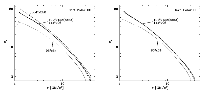
Figure 2: Radial profile of plasma $\beta$ (upper row) and electron temperature $\theta_{e}$ (lower row) for each resolution. The columns are for the soft-polar-boundary (left) and hard-polar-boundary (right).

Figure 2 shows the radial profile of $\beta$ and $\theta_{e}$ calculated using equation 9 for all the runs. All time averages run from $t=4000$ to the end of the run; at $t=4000$ the disk at $r\lesssim 10$ is in a steady state for all runs except for the lowest resolution model, which shows a clear upward trend in $\beta$ over the entire run. The lowest $(96\times 96\times 64)$ and medium $(144\times 144\times 96)$ resolution runs are averaged over 3 runs with different initial seeds to reduce run-to-run variation. The figure shows profiles for both the hard and the soft polar boundary conditions described in §2.

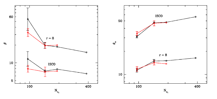
Figure 3: Plasma $\beta$ (left) and electron temperature $\theta_{e}$ (right) plotted as a function of resolution at the ISCO ($r=2.04$) and $r=8$. The black lines are for the soft-polar-boundary and the red lines are for the hard-polar-boundary.

Figure 3 shows $\beta$ and $\theta_{e}$ plotted against radial resolution $N_{x_{1}}$ for $r=2.04$ (ISCO) and $8$. The soft- and hard-polar boundary results are shown as solid black and red lines, respectively. Most quantities vary sharply from $N_{x_{1}}=96$ to $144$ and then far less at higher resolution. For example, the soft polar boundary models have $\beta(\text{ISCO})=(11.6,7.3,7.8,6.6)$, and $\theta_{e}(\text{ISCO})=(31,47,48,57)$ at the four resolutions.

Notice that at resolutions greater than $144\times 144\times 96$ there are only small quantitative differences between the hard- and soft-polar boundary conditions, as seen in Figure 2 and 3. We conclude that the effect of the polar boundary conditions on the main, equatorial flow is small for these dimensionless variables.

What part of the variations at $N_{x_{1}}\geq 144$ is real variation with resolution, and what part is run-to-run noise? The error bars in Figure 3 show standard deviation of the three runs performed for the lowest $(96\times 96\times 64)$ and medium $(144\times 144\times 96)$ data points with different initial seeds. Error bars are not available for the higher resolution data points due to computational expense. The size of the error bars is comparable to the differences between models run with different resolution. One might hope to gain additional information by measuring, e.g., $\beta$ at several radii and averaging the trend with resolution, but, interestingly, the entire radial profile varies in a correlated way. Nevertheless Figures 2 and 3 show a clear trend of decreasing $\beta$ and $\theta_{e}$ with increasing resolution. It seems likely, therefore, that there is a genuine but weak trend with resolution.

4 Correlation lengths

We have looked at one-point statistics for non-dimensional variables. What about two-point statistics, which measure the spatial structure of the turbulence, and in particular the correlation length? The correlation length is a natural measure of the outer scale of the turbulence, and should be resolved and independent of resolution in a converged simulation.

We consider only the azimuthal correlation length, as this is most straightforward to compute, and is most often under resolved in global simulations (HGK). The correlation function at radius $r$ on the equatorial plane is

$$R(\phi)=\int_{0}^{2\pi}\delta f(\phi_{0})\delta f(\phi_{0}+\phi)d\phi_{0}\;\text{,}$$ (13)

where $\delta f$ is deviation from average value of variable $f$ at r. In practice, we average $R$ in small area $r\Delta r\Delta\theta$ across the equatorial plane, normalize, and average in time:

$$\bar{R}(r,\phi,t) =\int_{r\pm\frac{\Delta r}{2},\;\pm\Delta\theta}R(r,\theta,\phi,t)rdrd\theta/(r\Delta r\Delta\theta)$$ (14)

$$\bar{R}(r,\phi) =\int_{t_{1}}^{t_{2}}R(r,\phi,t)/R(r,0,t)dt\;\text{.}$$ (15)

Note that the correlation function for magnetic field is defined as

$$R(\phi)=\int_{0}^{2\pi}\delta b^{\mu}(\phi_{0})\delta b_{\mu}(\phi_{0}+\phi)d\phi_{0}\;\text{,}$$ (16)

where $b^{\mu}$ is defined in §2. Then

$$\lambda:\bar{R}(r,\lambda)=\bar{R}(r,0)/e\;\text{.}$$ (17)

is the correlation length at radius $r$.

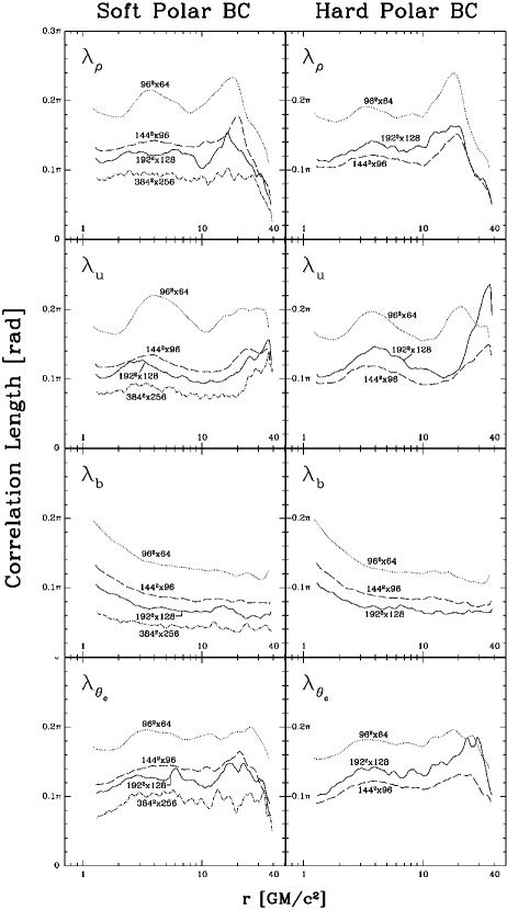
Figure 4: Azimuthal correlation length as a function of radius for each resolution. From the top panel, density ($\rho$), internal energy ($u$), magnetic field ($b$), and electron temperature ($\theta_{e}$). The left column is for the soft-polar-boundary and right column is for the hard-polar-boundary.

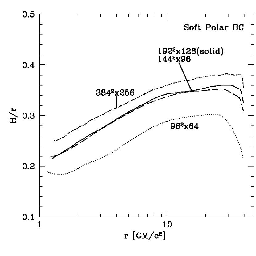
Figure 6: Radial profile of the scale height $H/r$ for the runs with the soft polar boundary. The runs with the hard polar boundary have similar profiles.

Figure 4 shows the azimuthal correlation length for density $\rho$, internal energy $u$, magnetic field $b$, and $\theta_{e}$ for all runs. Evidently the correlation lengths (angles) are nearly independent of $r$, except close to the outer boundary where the models are not in a steady state. The correlation length varies between about $0.2\pi$ at the lowest resolution to $0.1\pi$ at the highest resolution for all variables except $b$. Since $H/r\sim 0.3$ for all models over a wide range in radius (Figure 6), this corresponds (assuming flat space geometry) to $1$ to $2$ vertical scale heights.

The non-dimensional resolution $\lambda/\Delta\phi\simeq 12(\lambda/(H/r))(N_{x_{1}}/384)$ where $\Delta\phi=2\pi/N_{x_{3}}$, is marginal even for our highest resolution simulation. For $b$, the correlation length of the highest resolution is smaller than that for any other variable. The magnetic field structure is underresolved.

Figure 5 plots correlation length against resolution at the ISCO for the same variables as in Figure 4; here red is the hard polar boundary and black is the soft polar boundary. The dotted lines show how the correlation length would vary if it were fixed at $2,5$ and $10$ grid zones.

For $\rho$, $u$, and $\theta_{e}$ (the nonmagnetic variables) the correlation length is $\sim 5$ grid zones for the two lowest resolution simulations. At higher resolution– $N_{x_{1}}=192$ and $384$– the correlation length increases to $>10$ grid zones, and the slope of the change in correlation length with resolution decreases. This suggests that for the two highest resolution runs some structures in the turbulence are beginning to be resolved.

For $b$, on the other hand, the correlation length decreases nearly proportional to the grid scale, with the correlation length fixed at around $5$ grid zones per correlation length. There are small signs of an increase at the highest resolution, but in light of run-to-run variations the significance of this increase is marginal at best. The outer scale for the magnetic field is not resolved.

For all variables the correlation lengths for hard and soft boundary polar conditions are consistent. Evidently the polar boundary does not influence the structure of turbulence in the equatorial disk.

How do these correlation lengths correspond to those found in local model simulations? Guan et al. (2009) found in their unstratified shearing box model that the three dimensional correlation function was a triaxial ellipsoid elongated in the azimuthal direction and tilted into trailing orientation. The relationship between our azimuthal correlation length $\lambda_{b}$ and the Guan et al. (2009) results is

$$\lambda=\left(\frac{\cos^{2}\theta_{tilt}}{\lambda_{maj}^{2}}+\frac{\sin^{2}\theta_{tilt}}{\lambda_{min}^{2}}\right)^{-1/2}$$ (18)

where $\theta_{tilt}\approx 15\,\rm deg$ is the tilt angle of the correlation ellipse, and $\lambda_{maj}$, $\lambda_{min}$ are the major and minor axis of magnetic correlation lengths. For the best resolved net azimuthal field model in Guan et al. (2009) (y256b, which like our global models saturates at $\beta\simeq 20$), this implies $\lambda\simeq 0.17H\simeq 0.05\,\rm rad$, or $0.016\pi\,\rm rad$. Therefore, it is surprising that correlation length as large as $\simeq 0.3\,\rm rad\,\sim H$ are measured in our model for the nonmagnetic variables.

Davis et al. (2010) have computed correlation lengths in stratified, isothermal models with zero net flux. In a model run with athena at a resolution of 64 zones per scale height, the implied azimuthal correlation length (averaged over $-H<z<H$) for the magnetic field is slightly larger than in the unstratified models of Guan et al. (2009), about $0.23H$, or $0.02\pi\,\rm rad$. Guan & Gammie (2011) have also run stratified, isothermal models at lower resolution with a zeus type code. They find an implied azimuthal midplane correlation length (similarly averaged) for the magnetic field that is even larger, about $0.9H$, or $0.09\pi$ radians. Since correlation length decreases with increasing resolution it is possible that Guan & Gammie (2011) are not resolving the correlation length, and that at higher resolution the correlation length would be closer to that measured by Davis et al. (2010).

The correlation length of our highest resolution run spans $0.6(H/r)$ to $0.4(H/r)$ from ISCO to $r\sim 10$ where the corresponding $\beta$ is $7$ and $16$, respectively. This is larger than the stratified shearing box results of Davis et al. (2010) but smaller than that of Guan & Gammie (2011). To resolve the correlation length found in Davis et al. (2010) we would need another factor of $2$ in linear resolution. Note that recently Beckwith et al. (2011) found in their global thin disk MHD simulation that azimuthal correlation length to be about $1.3(H/r)$ by averaging $|z|<H$ and $5<r<11$. This is larger than our result but also falls between Davis et al. (2010) and Guan & Gammie (2011).

5 Spectra

An interesting application of GRMHD models is to simulate observations of sources such as Sgr A* (Dolence et al., 2009; Moscibrodzka et al., 2010; Hilburn et al., 2010; Dexter et al., 2009, 2010; Dexter & Fragile, 2011). Are the simulated spectra converged?

The dynamical models underlying the spectral models are run with zero cooling, and the spectra are produced in a post-processing step. This is self-consistent as long as the flows are advection dominated: the accretion timescale is much shorter than the cooling timescale. We calculate the emergent radiation using grmonty, a general relativistic Monte Carlo radiative transfer code (Dolence et al., 2009).

grmonty makes no symmetry assumptions and includes synchrotron emission, absorption, and Compton scattering. Using the rest-frame emissivity for a hot, thermal plasma (Leung et al., 2011) the code produces Monte Carlo samples of the emitted photons–“superphotons” that carry a “weight” representing the number of photons per superphoton. The superphotons follow geodesics, with weight varying continuously due to synchrotron absorption. They also Compton scatter and produce new, scattered superphotons with weight proportional to the scattering probability. We use a “fast light” approximation, where for each snapshot of simulation data a spectrum is created by treating the fluid variables as if they were time-independent. This approximation is excellent for the time-averaged spectra we consider here. Superphotons that reach large radius are collected in poloidally and azimuthally distributed bins, and each bin produces a spectrum. A complete description of the code is given in Dolence et al. (2009).

To compare runs we generate spectra for $200-1200$ time slices (depending on the length of the run) and time-average them. The spectrum of each time slice is produced from azimuthally averaged bins that extend from $0.12\pi<|\theta-\pi/2|<0.18\pi\,\rm rad$ with respect to the equatorial plane.

We modify the simulation-provided data in one respect before calculating the spectrum. The quality of the non-magnetic fluid variable integration in the funnel region is poor due to truncation error. In particular the temperature can be high ($\theta_{e}>10^{4}$) and the particle density is determined entirely by a density floor in HARM3D. We therefore zero the emissivity if $b^{2}/\rho>1$ to avoid contaminating the spectrum with possibly unphysical emission.

It is necessary to fix a mass, length, and time unit to generate a radiative model. The combination $GM_{BH}$ sets a length and time scale but not a mass scale because the mass of the accretion flow is negligible in comparison to the black hole. We set $M_{BH}=4.5\times 10^{6}M_{\odot}$, comparable to the mass of SgrA*. The mass unit for the torus $\mathcal{M}$ is still free; we set it so that the $1.3\,{\rm mm}$ flux matches the observed flux from Sgr A* of $\simeq 3.4\,{\rm Jy}$ (Marrone et al., 2006).

We want to model emission from a statistically stationary accretion flow. Because we start with a finite mass torus and it accretes over time, however, there is a steady decrease in density, field strength, accretion rate, etc., as the simulation progresses. We scale away this long term evolution using a smooth model, as follows. We set the mass unit $\mathcal{M}=M_{0}s(t)$ where $M_{0}$ is a constant and $s(t)$ is a two-parameter scaling function. Then

$$\rho_{unit}=\mathcal{M}/(\frac{GM_{\textrm{BH}}}{c^{2}})^{3}\quad\quad u_{unit}=\rho_{unit}c^{2}\quad\quad B_{unit}=c\sqrt{4\pi\rho_{unit}}\;\text{,}$$ (19)

or expressing with $s(t)$,

$$\rho_{unit}=\rho_{0}s(t)\quad\quad u_{unit}=u_{0}s(t)\quad\quad B_{unit}=B_{0}\sqrt{s(t)}$$ (20)

where they are the unit mass density, internal energy, and magnetic field strength, respectively, and $\rho_{0}$, $u_{0}$, and $B_{0}$ are constants. Conversion from the simulation unit to the cgs unit is, e.g. $\rho_{cgs}=\rho_{sim}\rho_{unit}$.

The scaling function we employ has a form

$$\frac{1}{s(t)}=At^{-5/3}\exp{\left(-\frac{t_{\nu}}{t}\right)}$$ (21)

where $A$ and $t_{\nu}$ are free parameters determined by a fit to the numerical evolution. The form comes from fitting 1-d relativistic viscous disk models (see Dolence et al. 2011 in prep. for more complete discussion). Notice that without this time-dependent scaling procedure, or with a different scaling procedure, the spectra would vary systematically over the course of the simulation. The spectra would also differ systematically with resolution because the plasma $\beta$ varies with resolution.

We fit for $A$ and the viscous timescale $t_{\nu}$ from simulation data after a quasi-steady state has been reached, typically from $t=2000$ onwards. A sample fit to $\dot{M}$, for the $192\times 192\times 128$ run, is shown in Figure 7. The variance of the normalized accretion rate decreases with resolution, that is, at higher resolution the fluctuations are smaller and equation 21 gives an increasingly good fit. The maximum of the normalized accretion rate is nearly independent of resolution, when models with different resolution are compared over the same time interval.

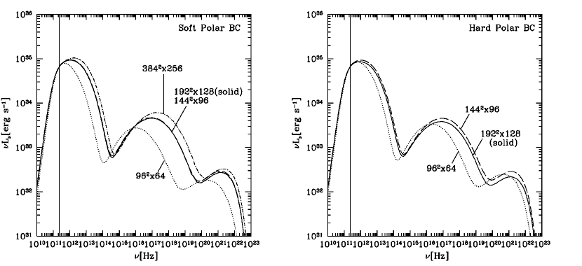
Figure 8: Spectra for each resolution. Flux is fixed to $3.4\,{\rm Jy}$ at $1.3\,{\rm mm}$ shown by the vertical solid line. The left plot is for the soft-polar-boundary and right plot is for the hard-polar-boundary.

Broadband, time-averaged synthetic spectra are shown in Figure 8. The mass unit of the torus is fixed by the condition that $f_{\nu}(230\,{\rm GHz})=3.4\,{\rm Jy}$ for a Sgr A* model measured at the solar circle. The shape of the spectrum is broadly similar at all resolutions for both polar boundary conditions.

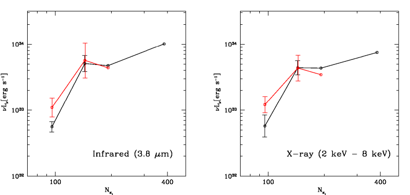
Figure 9: Infrared flux density ($3.8\,\rm\mu\rm m$, left) and X-ray flux (integrated from $2\,\rm keV$ to $8\,\rm keV$, right) as a function of resolution. The black lines are for the soft-polar-boundary and the red lines are for the hard-polar-boundary.

Figure 9 shows flux density plotted against resolution in the infrared ($3.8\,\rm\mu\rm m$) and X-ray (integrated from $2\,\rm keV$ to $8\,\rm keV$) where most of the emission is from direct synchrotron and single Compton scatterings, respectively. Some of the variation is likely due to run-to-run variation, as indicated by the error bars on the $N_{x_{1}}=96$ and $N_{x_{1}}=144$ models. The flux varies with resolution by less than about 50% at infrared and 30% at X-ray for $N_{x_{1}}>144$. The spectra therefore appear remarkably consistent and independent of resolution, at least for the $M$ and $\dot{M}$ appropriate to Sgr A*.

In a sense this is not surprising, because (1) our normalization procedure removes much of the variation that might arise from the decrease of $\beta$ with resolution, and (2) the temperature is very well converged. The combined effect of the fixed flux normalization and the variation with resolution is to strengthen the magnetic field slightly and move the synchrotron peak slightly further into the infrared. This is echoed in the first Compton bump in the X-ray, which is forced to slightly higher energy by the increase in infrared input photons. While we have demonstrated this for only a single set of the model parameters ($M$, $f_{\nu}(230\,{\rm GHz})$), exploration of slightly different models with similarly consistent results shows that this is not a unique case.

6 Summary

We have investigated convergence of global GRMHD simulations of hot accretion flows onto a black hole and the emergent spectrum. We have run GRMHD simulations for four different resolutions, $96\times 96\times 64$, $144\times 144\times 96$, $192\times 192\times 128$, $384\times 384\times 256$ in spherical-polar coordinates. We have probed convergence using three diagnostics: time-averaged radial profiles of nondimensional quantities (plasma $\beta$ and electron temperature $\theta_{e}$); azimuthal correlation lengths for several variables including the magnetic field; and artificial spectra generated with a Monte Carlo code.

For most of our diagnostics there are substantial differences between the lowest $(96\times 96\times 64)$ and next lowest $(144\times 144\times 96)$ resolution, and relative minor changes at higher resolution. Run-to-run variations in the lower resolution models tend to be larger than the differences between the higher resolution $(192\times 192\times 128$ and $384\times 384\times 256)$ models.

We find that the magnetic correlation length is not converged. It decreases nearly linearly with resolution, with the number of grid cells per magnetic correlation length fixed at $\sim 5$, although we do see a slight increase as resolution increases. Comparison with local model/shearing box simulations suggests that the turbulence does not change qualitatively at higher resolution. Such comparisons also suggest that another factor of $\approx 2$ in linear resolution (costing about $1.6\times 10^{7}$ cpu-hours) would resolve the azimuthal magnetic correlation length. None of the existing simulations (local or global) resolve scales more than a factor of $\approx 4$ smaller than the correlation length (particularly the minor axis correlation length, which is oriented nearly along the radial unit vector and which we have not investigated here). If we identify the correlation length with the outer scale of MRI driven turbulence, as seems reasonable, then none of these models have a resolved inertial range.

On the other hand, time-averaged synthetic spectra based on the GRMHD models, with parameters fixed to match Sgr A*, are remarkably reproducible from resolution to resolution. This suggests that simulated observations from existing simulations have some predictive power. We think it likely that the leading source of error in the high resolution radiative models is now related to the underlying physical model (particularly the fluid model treatment of the plasma, and the absence of conduction) rather than the finite resolution of the models.

A similar convergence study has been conducted by HGK for nonrelativistic global models. It is worth asking whether our models are converged according to the dimensionless resolution $Q$, the ratio of most unstable MRI wavelength to the grid cell size in the azimuthal and vertical direction. In the azimuthal direction,

$$Q_{3}= \frac{\lambda_{MRI}}{r\Delta\phi}\simeq 2\pi\left(\frac{H}{r}\right)\frac{|B_{3}|}{c_{s}\sqrt{2\rho}}\frac{1}{\Delta\phi}$$ (22)

$$\simeq 2\pi\left(\frac{H}{r}\right)\beta^{-1/2}\frac{1}{\Delta\phi}$$ (23)

($Q_{y}$ or $Q_{\phi}$ in HGK’s notation), where $c_{s}\sim H\Omega$ is the sound speed. This gives $Q_{3}\gtrsim 22$ and $\gtrsim 10$ for $N_{x_{1}}=384$ and $192$, respectively, for all radii less than $10$. In the vertical direction,

$$Q_{2}\simeq 2\pi\left(\frac{H}{r}\right)\frac{|B_{2}|}{c_{s}\sqrt{2\rho}}\frac{1}{\Delta\theta}=Q_{3}\frac{|B_{2}|}{|B_{3}|}$$ (24)

($Q_{z}$ in HGK’s notation) where $\Delta\theta$ is the zone size in Kerr-Schild coordinates at the midplane. Since $|B_{2}/B_{3}|$ is usually $\sim 3-10$, this gives $Q_{2}\gtrsim 70$ and $\gtrsim 30$ for $N_{x_{1}}=384$ and $192$, respectively, for all $r<10$. The required $Q$ values to resolve the characteristic wavelength are $Q_{2}\gtrsim 20-60$ and $Q_{3}\gtrsim 6$. Hence, MRI in the toroidal direction is resolved but not in the poloidal direction in these runs according to HGK’s $Q$ criterion.

To summarize our findings in the form of guidance for future simulators: (1) the resolution $96\times 96\times 64$ is too low. The convergence measurements differ by factors of several from the highest resolution runs, and the magnetic field weakens steadily in a relative sense ($\beta$ increases) over the course of the run; (2) the resolution $144\times 144\times 96$ shows early signs of convergence except for the correlation length of the magnetic field; (3) the resolution $192\times 192\times 128$ and $384\times 384\times 256$ differ relatively little from each other and show signs of convergence in the azimuthal correlation lengths, the temperature, and spectra, but not in the correlation length of magnetic field; (4) the observed trends with increasing resolution (to the extent that they are significant at the highest resolution) are that $\beta$ decreases, $\theta_{e}$ increases, correlation lengths decreases, and IR and X-ray fluxes increase relative to millimeter fluxes, which we use to normalize the spectrum.

Figure 1: Poloidal slices of the initial and turbulent state of the global simulation. The pseudo-color is showing scaled logarithmic density and black lines are the initial magnetic field lines.

Figure 5: At ISCO, azimuthal correlation length of density ($\lambda_{\rho}$), internal energy ($\lambda_{u}$), magnetic field ($\lambda_{b}$), and electron temperature ($\theta_{e}$) are plotted as a function of resolution. The black lines are for the soft-polar-boundary and the red lines are for the hard-polar-boundary. Black dotted lines show a correlation length of 2, 5, and 10 grid cells, to which correlation length size of 2, 5, and 10 grids correspond at each resolution in azimuthal direction.

Figure 7: Time evolution of accretion rate for the run $192\times 192\times 128$ with hard polar boundary. Dotted line is the actual accretion rate and the solid line is a fit of the form shown in equation (21).

References

- Anninos et al. (2005) Anninos, P., Fragile, P. C., & Salmonson, J. D. 2005, ApJ, 635, 723
- Balbus & Hawley (1991) Balbus, S. A., & Hawley, J. F. 1991, ApJ, 376, 214
- Beckwith et al. (2011) Beckwith, K., Armitage, P. J., & Simon, J. B. 2011, arXiv:1105.1789
- Beckwith et al. (2009) Beckwith, K., Hawley, J. F., & Krolik, J. H. 2009, ApJ, 707, 428
- Beckwith et al. (2008) Beckwith, K., Hawley, J. F., & Krolik, J. H. 2008, ApJ, 678, 1180
- Brandenburg (1996) Brandenburg, A. 1996, ApJ, 465, L115
- Davis et al. (2010) Davis, S. W., Stone, J. M., & Pessah, M. E. 2010, ApJ, 713, 52
- De Villiers & Hawley (2003) De Villiers, J.-P., & Hawley, J. F. 2003, ApJ, 592, 1060
- De Villiers et al. (2003) De Villiers, J.-P., Hawley, J. F., & Krolik, J. H. 2003, ApJ, 599, 1238
- Dexter et al. (2009) Dexter, J., Agol, E., & Fragile, P. C. 2009, ApJ, 703, L142
- Dexter et al. (2010) Dexter, J., Agol, E., Fragile, P. C., & McKinney, J. C. 2010, ApJ, 717, 1092
- Dexter & Fragile (2011) Dexter, J., & Fragile, P. C. 2011, ApJ, 730, 36
- Dolence et al. (2009) Dolence, J. C., Gammie, C. F., Mościbrodzka, M., & Leung, P. K. 2009, ApJS, 184, 387
- Fishbone & Moncrief (1976) Fishbone, L. G., & Moncrief, V. 1976, ApJ, 207, 962
- Flock et al. (2011) Flock, M., Dzyurkevich, N., Klahr, H., Turner, N. J., & Henning, T. 2011, arXiv:1104.4565
- Fragile et al. (2007) Fragile, P. C., Blaes, O. M., Anninos, P., & Salmonson, J. D. 2007, ApJ, 668, 417
- Fragile & Meier (2009) Fragile, P. C., & Meier, D. L. 2009, ApJ, 693, 771
- Fragile et al. (2009) Fragile, P. C., Lindner, C. C., Anninos, P., & Salmonson, J. D. 2009, ApJ, 691, 482
- Fromang & Papaloizou (2007) Fromang, S., & Papaloizou, J. 2007, A&A, 476, 1113
- Fromang et al. (2007) Fromang, S., Papaloizou, J., Lesur, G., & Heinemann, T. 2007, A&A, 476, 1123
- Fromang (2010) Fromang, S. 2010, A&A, 514, L5
- Gammie (2004) Gammie, C. F. 2004, ApJ, 614, 309
- Gammie et al. (2003) Gammie, C. F., McKinney, J. C., & Tóth, G. 2003, ApJ, 589, 444
- Gammie et al. (2004) Gammie, C. F., Shapiro, S. L., & McKinney, J. C. 2004, ApJ, 602, 312
- Goldreich & Lynden-Bell (1965) Goldreich, P., & Lynden-Bell, D. 1965, MNRAS, 130, 97
- Goldreich & Tremaine (1978) Goldreich, P., & Tremaine, S. 1978, ApJ, 222, 850
- Guan et al. (2009) Guan, X., Gammie, C. F., Simon, J. B., & Johnson, B. M. 2009, ApJ, 694, 1010
- Guan & Gammie (2011) Guan, X., & Gammie, C. F. 2011, ApJ, 728, 130
- Hawley & Balbus (1991) Hawley, J. F., & Balbus, S. A. 1991, ApJ, 376, 223
- Hawley & Balbus (1992) Hawley, J. F., & Balbus, S. A. 1992, ApJ, 400, 595
- Hawley et al. (1995) Hawley, J. F., Gammie, C. F., & Balbus, S. A. 1995, ApJ, 440, 742
- Hawley et al. (1996) Hawley, J. F., Gammie, C. F., & Balbus, S. A. 1996, ApJ, 464, 690
- Hawley et al. (2011) Hawley, J. F., Guan, X., & Krolik, J. H. 2011, arXiv:1103.5987
- Hilburn et al. (2010) Hilburn, G., Liang, E., Liu, S., & Li, H. 2010, MNRAS, 401, 1620
- Hirose et al. (2004) Hirose, S., Krolik, J. H., De Villiers, J.-P., & Hawley, J. F. 2004, ApJ, 606, 1083
- Hirose et al. (2006) Hirose, S., Krolik, J. H., & Stone, J. M. 2006, ApJ, 640, 901
- Leung et al. (2011) Leung, P. K., Gammie, C. F. & Noble, S. C. 2011
- Lesur & Longaretti (2007) Lesur, G., & Longaretti, P.-Y. 2007, MNRAS, 378, 1471
- Marrone et al. (2006) Marrone, D. P., Moran, J. M., Zhao, J.-H., & Rao, R. 2006, Journal of Physics Conference Series, 54, 354
- Matsumoto et al. (1996) Matsumoto, R., Uchida, Y., Hirose, S., Shibata, K., Hayashi, M. R., Ferrari, A., Bodo, G., & Norman, C. 1996, ApJ, 461, 115
- McKinney (2006) McKinney, J. C. 2006, MNRAS, 368, 1561
- McKinney & Gammie (2004) McKinney, J. C., & Gammie, C. F. 2004, ApJ, 611, 977
- Misner et al. (1973) Misner, C., Thorne, K., & Wheeler, J. 1973, Gravitation (NewYork: Freeman)
- Moscibrodzka et al. (2010) Moscibrodzka, M., Gammie, C. F., Dolence, J., Shiokawa, H., & Leung, P. K. 2010, arXiv:1002.1261
- Narayan et al. (1987) Narayan, R., Goldreich, P., & Goodman, J. 1987, MNRAS, 228, 1
- Noble et al. (2006) Noble, S. C., Gammie, C. F., McKinney, J. C., & Del Zanna, L. 2006, ApJ, 641, 626
- Noble et al. (2009) Noble, S. C., Krolik, J. H., & Hawley, J. F. 2009, ApJ, 692, 411
- Noble et al. (2010) Noble, S. C., Krolik, J. H., & Hawley, J. F. 2010, ApJ, 711, 959
- Noble et al. (2007) Noble, S. C., Leung, P. K., Gammie, C. F., & Book, L. G. 2007, Classical and Quantum Gravity, 24, 259
- Penna et al. (2010) Penna, R. F., McKinney, J. C., Narayan, R., Tchekhovskoy, A., Shafee, R., & McClintock, J. E. 2010, MNRAS, 408, 752
- Sano et al. (2004) Sano, T., Inutsuka, S.-i., Turner, N. J., & Stone, J. M. 2004, ApJ, 605, 321
- Schnittman et al. (2006) Schnittman, J. D., Krolik, J. H., & Hawley, J. F. 2006, ApJ, 651, 1031
- Shafee et al. (2008) Shafee, R., McKinney, J. C., Narayan, R., Tchekhovskoy, A., Gammie, C. F., & McClintock, J. E. 2008, ApJ, 687, L25
- Shcherbakov et al. (2010) Shcherbakov, R. V., Penna, R. F., & McKinney, J. C. 2010, arXiv:1007.4832
- Simon et al. (2011) Simon, J. B., Hawley, J. F., & Beckwith, K. 2011, ApJ, 730, 94
- Stone et al. (1996) Stone, J. M., Hawley, J. F., Gammie, C. F., & Balbus, S. A. 1996, ApJ, 463, 656
- Tóth (2000) Tóth, G. 2000, Journal of Computational Physics, 161, 605