Microscopic approach to large-amplitude deformation dynamics with local QRPA inertial masses

Abstract

We have developed a new method for determining microscopically the five-dimensional quadrupole collective Hamiltonian, on the basis of the adiabatic self-consistent collective coordinate method. This method consists of the constrained Hartree-Fock-Bogoliubov (HFB) equation and the local QRPA (LQRPA) equations, which are an extension of the usual QRPA (quasiparticle random phase approximation) to non-HFB-equilibrium points, on top of the CHFB states. One of the advantages of our method is that the inertial functions calculated with this method contain the contributions of the time-odd components of the mean field, which are ignored in the widely-used cranking formula. We illustrate usefulness of our method by applying to oblate-prolate shape coexistence in ⁷²Kr and shape phase transition in neutron-rich Cr isotopes around $N=40$.

1 Introduction

The five-dimensional (5D) quadrupole collective Hamiltonian is a powerful tool to describe large-amplitude deformation dynamics including triaxial shape degree of freedom as well as axially symmetric deformation. The 5D quadrupole collective Hamiltonian is characterized by seven functions: the collective potential, three vibrational and three rotational inertial functions (collective masses). To calculate the inertial functions, the Inglis-Belyaev (IB) cranking formula [1, 2] has been widely used. However, it is well known that IB cranking masses do not contain the contributions from the time-odd components of the mean field and underestimate the collective masses.

In this presentation, we introduce a new method of determining microscopically the collective potential and the inertial functions which can overcome the shortcoming of the IB cranking formula. This method is derived from the adiabatic self-consistent collective coordinate (ASCC) method [3, 4], which is based on the adiabatic time-dependent Hartree-Fock-Bogoliubov (TDHFB) theory and, with which one can extract the collective subspace (collective manifold) from the large-dimensional TDHFB configuration space. The method we employ in this study is the version of the ASCC method simplified by assuming the one-to-one correspondence between the collective manifold and the quadrupole deformation parameter space $(\beta,\gamma)$. The main concept of this method is the local normal modes on top of the constrained Hartree-Fock-Bogoliubov (CHFB) states at every point of the $(\beta,\gamma)$ plane. In this method, we first solve the CHFB equations imposing the constraints on the proton and neutron numbers and deformation parameters $(\beta,\gamma)$. Then, we solve local QRPA (quasiparticle random-phase approximation) equations, which are an extension of the usual QRPA to the non-HFB-equilibrium points. Hereafter, we call the method “the constrained HFB plus local QRPA (CHFB+LQRPA) method.”

We shall show some results of the applications of the CHFB+LQRPA method to the oblate-prolate shape coexistence in ⁷²Kr and to the shape phase transition in neutron-rich Cr isotopes around $N=40$.

2 Theoretical framework

Here, we briefly explain the theoretical framework of the CHFB+LQRPA method (see Ref. [5] for details). The 5D quadrupole collective Hamiltonian is written in terms of the magnitude $\beta$, the degree of triaxiality $\gamma$ of quadrupole deformation, three Euler angles, and their time derivatives as

$$\mathcal{H}_{\rm coll} =T_{\rm vib}+T_{\rm rot}+V(\beta,\gamma),$$ (1)

$$T_{\rm vib} =\frac{1}{2}D_{\beta\beta}(\beta,\gamma)\dot{\beta}^{2}+D_{\beta\gamma}(\beta,\gamma)\dot{\beta}\dot{\gamma}+\frac{1}{2}D_{\gamma\gamma}(\beta,\gamma)\dot{\gamma}^{2},$$ (2)

$$T_{\rm rot} =\frac{1}{2}\sum_{k=1}^{3}{\cal J}_{k}(\beta,\gamma)\omega^{2}_{k},$$ (3)

where $T_{\rm vib}$, $T_{\rm rot}$ and $V$ represent the vibrational, rotational and collective potential energies, respectively. We determine the three vibrational inertial masses, three rotational moments of inertia, and collective potential in the collective Hamiltonian, by solving the CHFB+LQRPA equations.

In the CHFB+LQRPA method, we first solve the CHFB equation to determine the collective potential $V(\beta,\gamma)$:

$$\delta\left\langle\phi(\beta,\gamma)\right|\hat{H}_{\rm CHFB}(\beta,\gamma)\left|\phi(\beta,\gamma)\right\rangle=0,$$ (4)

where $\hat{H}_{\rm CHFB}=\hat{H}-\sum_{\tau}\lambda^{(\tau)}\tilde{N}^{(\tau)}-\sum_{m}\mu^{(m)}\hat{D}_{2m}$. Then, we solve the LQRPA equations on top of the CHFB states obtained above,

$$\delta \left\langle\phi(\beta,\gamma)\right|[\hat{H}_{\rm CHFB}(\beta,\gamma),\hat{Q}^{i}(\beta,\gamma)]-\frac{1}{i}\hat{P}_{i}(\beta,\gamma)\left|\phi(\beta,\gamma)\right\rangle=0,$$ (5)

$$\delta \left\langle\phi(\beta,\gamma)\right|[\hat{H}_{\rm CHFB}(\beta,\gamma),\frac{1}{i}\hat{P}_{i}(\beta,\gamma)]-C_{i}(\beta,\gamma)\hat{Q}^{i}(\beta,\gamma)\left|\phi(\beta,\gamma)\right\rangle=0,\quad\quad(i=1,2).$$ (6)

The vibrational inertial functions are calculated by transforming two LQRPA modes to the $(\beta,\gamma)$ degrees of freedom. We also solve the LQRPA equations for rotation to determine the moments of inertia. In this work, we adopt a version of the pairing-plus-quadrupole (P+Q) interaction including the quadrupole pairing interaction as well as the monopole pairing interaction and take two major harmonic oscillator shells as a model space.

Finally, we solve the collective Schrödinger equation for the 5D quadrupole collective Hamiltonian quantized according to Pauli’s prescription to obtain the excitation energies and collective wave functions, with which the electric quadrupole transitions and moments are calculated.

3 Application to oblate-prolate shape coexistence in ⁷²Kr

In this section, we briefly show the numerical results of the application of the CHFB+LQRPA method to oblate-prolate shape coexistence in ⁷²Kr. The effective charges are adjusted to $(e^{(n)}_{\rm eff},e^{(p)}_{\rm eff})=(0.658,1.658)$ such that the calculated result of $B(E2;2_{1}^{+}\rightarrow 0_{1}^{+})$ reproduces the experimental value for ⁷⁴Kr [7]. The detailed results of this calculation are shown in Ref. [6] together with the results for ^74,76Kr.

Figure 1 shows the collective potential $V(\beta,\gamma)$, the vibrational inertial function $D_{\beta\beta}(\beta,\gamma)$, and the rotational moment of inertia $\mathcal{J}_{1}(\beta,\gamma)$ for ⁷²Kr. The collective potential has two local minima: the oblate minimum is lower than the prolate one. The spherical shape is a local maximum. One can see that $D_{\beta\beta}$ indicates strong $\beta-\gamma$ dependence and that the moment of inertia ${\cal J}_{1}$ deviates strongly from the irrotational moment of inertia. In Ref. [6], we have seen the collective wave function is localized on the oblate (prolate) side in the $(\beta,\gamma)$ plane in the ground (excited) band and that the localization of the wave function develops with increasing angular momentum. The development of the localization is strongly related to the $\beta-\gamma$ dependence of the moments of inertia seen in Fig. 1(c).

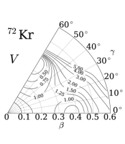
(a) $V(\beta,\gamma)$

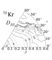
(b) $D_{\beta\beta}(\beta,\gamma)$

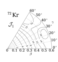
(c) ${\cal J}_{1}(\beta,\gamma)$

Figure 1: Collective potential energy surfaces $V(\beta,\gamma)$ in units of MeV, LQRPA vibrational inertial mass $D_{\beta\beta}(\beta,\gamma)$ and LQRPA rotational moment of inertia ${\cal J}_{1}(\beta,\gamma)$ in unit of MeV^-1 for ⁷²Kr.

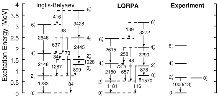
Figure 2: Excitation spectra and $B(E2)$ values calculated for ⁷²Kr by means of the CHFB+LQRPA method (denoted LQRPA) and experimental data [8, 9, 10]. For comparison, results calculated using the IB cranking masses (denoted Inglis-Belyaev) are also shown. Only $B(E2)$’s larger than 1 Weisskopf unit are shown in units of $e^{2}{\rm fm}^{4}$.

In Fig. 2, the excitation energies and $B(E2)$ values for ⁷²Kr are shown together with the experimental data. We show the result obtained using the IB cranking masses for comparison. The excitation energies obtained with the LQRPA masses are lower than those obtained with the IB cranking masses and agree better with the experimental data except for the $2_{1}^{+}$ state. In particular, the observed $0_{2}^{+}$ excitation energy which is close to the $2_{1}^{+}$ excitation energy is well reproduced with the LQRPA masses. One can see from the $E2$ transition strengths in Fig. 2 that the shape-coexistence-like character becomes stronger with increasing angular momentum: the interband transitions between the initial and final states having equal angular momentum become weaker and weaker, which reflects the development of the localization of the vibrational wave function mentioned above.

4 Application to shape transition in neutron-rich Cr isotopes

In this section, we shall show the results of the application to the CHFB+LQRPA method to shape phase transition in neutron-rich Cr isotopes around $N=40$, where the development of deformation has been suggested by recent experimental data. More details will be discussed in our forthcoming paper [11].

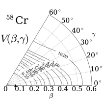
(a) ⁵⁸Cr

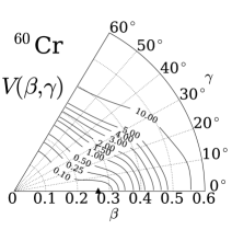
(b) ⁶⁰Cr

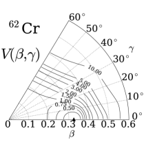
(c) ⁶²Cr

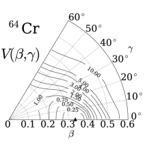
(d) ⁶⁴Cr

Figure 3: Collective potential energy surfaces $V(\beta,\gamma)$ for ^58-64Cr in units of MeV. The triangle denotes the position of the absolute minimum.

In this calculation, we have determined the interaction parameters as follows: the parameters for ⁶²Cr are determined such that the calculated monopole pairing gaps and deformation at the HFB equilibrium point as well as the pairing gaps at the spherical shape reproduce those obtained with the Skyrme-HFB calculation with the SkM* functional using the HFBTHO code [12]. For the other nuclei ^58,60,64,66Cr, we assume the simple mass number dependence according to Baranger and Kumar [13]. We take two major harmonic oscillator shells with $N=3,4$ and $N=2,3$ for neutrons and protons, respectively. The single particle energies are determined from those obtained with the constrained Skyrme-HFB calculation at spherical shape. We scale them according to the effective mass of the SkM* functional $m^{*}/m=0.79$. For the calculation of the $E2$ transitions and moments, we have used a standard value of the effective charges $(e^{(n)}_{\rm eff},e^{(p)}_{\rm eff})=(0.5,1.5)$ .

We show the collective potentials for ^58-64Cr in Fig. 3. The location of the absolute minimum is indicated by the triangle. In ⁵⁸Cr, the absolute minimum is located at a nearly spherical shape. Although the minimum shifts to larger $\beta$ in ⁶⁰Cr, the potential is extremely soft in the $\beta$ direction. In ⁶²Cr, a more definite local minimum appears and the minimum gets still deeper in ⁶⁴Cr. The potential energy surfaces seem to indicate a shape transition from a spherical to a prolately deformed shape along the isotopic chain toward $N=40$.

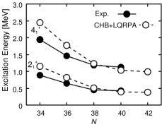
(a) $E(2_{1}^{+})$

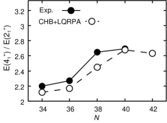
(b) $R_{4/2}$

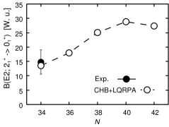
(c) $B(E2;2_{1}^{+}\rightarrow 0_{1}^{+})$

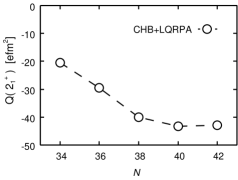
(d) $Q(2_{1}^{+})$

Figure 4: Excitation energies of the $2_{1}^{+}$ and $4_{1}^{+}$ states, their ratios $R_{4/2}$, $B(E2;2_{1}^{+}\rightarrow 0_{1}^{+})$, and the spectroscopic quadrupole moments of the $2_{1}^{+}$ states in comparison with the available experimental data [14, 15, 16, 17]. The $B(E2)$ values are shown in Weisskopf units.

We show in Fig. 4 the calculated excitation energies of the $2_{1}^{+}$ and $4_{1}^{+}$ states, their ratios $R_{4/2}=E(4_{1}^{+})/E(2_{1}^{+})$, $B(E2;2_{1}^{+}\rightarrow 0_{1}^{+})$, and the spectroscopic quadrupole moments of the $2_{1}^{+}$ states $Q(2_{1}^{+})$ calculated for ^58-66Cr in comparison with the available experimental data. Both of the experimental excitation energies and $R_{4/2}$ are reproduced well. The decrease in the excitation energies and the increase in $R_{4/2}$ reflect the development of deformation with increasing the neutron number. The $E2$ transition and moments also indicate the enhancement of collectivity: the magnitude of $B(E2)$ and $Q(2_{1}^{+})$ increase as the neutron number increases and they take a maximum at $N=40$. (Note that $Q(2_{1}^{+})$’s are negative indicating prolate shapes.) To sum up, our result suggests the development of prolate deformation from $N=34$ to $N=40$ and the largest collectivity at $N=40$.

5 Concluding Remarks

We have proposed the CHFB+LQRPA method for determining the inertial functions in the 5D quadrupole collective Hamiltonian, with which one can take into account the contributions from the time-odd components of the mean field to the inertial functions. We applied this method to the oblate-prolate shape coexistence in the low-lying states of ⁷²Kr and shape transition in neutron-rich Cr isotopes around $N=40$. The calculated results are in good agreement with the available experimental data.

The CHFB+LQRPA method is based on the ASCC method and it can be used in conjunction with any interaction in principle. Nevertheless, in this study, we have employed a rather simple interaction, the P+Q model including the quadrupole pairing interaction, for simplicity. The implementation with modern energy density functionals, such as Skyrme energy functionals and density-dependent pairing interaction is an issue for future under progress.

One of the authors (N. H.) is supported by the Special Postdoctoral Researcher Program of RIKEN. The numerical calculations were carried out on SR16000 at Yukawa Institute for Theoretical Physics in Kyoto University and RIKEN Cluster of Clusters (RICC) facility. This work is supported by KAKENHI (Nos. 21340073 and 20105003).

References

References

- [1] Inglis D R 1954 Phys. Rev. 96 1059
- [2] Beliaev S 1961 Nucl. Phys. 24 322
- [3] Matsuo M, Nakatsukasa T and Matsuyanagi K 2000 Prog. Theor. Phys. 103 959
- [4] Hinohara N, Nakatsukasa T, Matsuo M and Matsuyanagi K 2007 Prog. Theor. Phys. 117 451
- [5] Hinohara N, Sato K, Nakatsukasa T, Matsuo M and Matsuyanagi K 2011 Phys. Rev. C 82 064313
- [6] Sato K and Hinohara N 2011 Nucl. Phys. A 849 53
- [7] Clément E et al 2007 Phys. Rev. C 75 054313
- [8] Bouchez E et al 2003 Phys. Rev. Lett. 90 8
- [9] Gade A et al 2005 Phys. Rev. Lett. 95 022502
- [10] Fischer S M, Lister C J and Balamuth D P 2003 Phys. Rev. C 67 064318
- [11] Sato K et al 2011 in preparation
- [12] Stoitsov M, Dobaczewski J, Nazarewicz W and Ring P 2005 Comp. Phys. Comm. 167 43
- [13] Baranger M and Kumar K 1968 Nucl. Phys. A 110 490
- [14] Bürger A et al 2005 Phys. Lett. B 622 29
- [15] Zhu S et al 2006 Phys. Rev. C 74 064315
- [16] Aoi N et al 2009 Phys. Rev. Lett. 102 2
- [17] Gade A et al 2010 Phys. Rev. C 81 051304(R)