Hybridization of wave functions in one-dimensional localization

Abstract

A quantum particle can be localized in a disordered potential, the effect known as Anderson localization. In such a system, correlations of wave functions at very close energies may be described, due to Mott, in terms of a hybridization of localized states. We revisit this hybridization description and show that it may be used to obtain quantitatively exact expressions for some asymptotic features of correlation functions, if the tails of the wave functions and the hybridization matrix elements are assumed to have log-normal distributions typical for localization effects. Specifically, we consider three types of one-dimensional systems: a strictly one-dimensional wire and two quasi-one-dimensional wires with unitary and orthogonal symmetries. In each of these models, we consider two types of correlation functions: the correlations of the density of states at close energies and the dynamic response function at low frequencies. For each of those correlation functions, within our method, we calculate three asymptotic features: the behavior at the logarithmically large “Mott length scale”, the low-frequency limit at length scale between the localization length and the Mott length scale, and the leading correction in frequency to this limit. In the several cases, where exact results are available, our method reproduces them within the precision of the orders in frequency considered.

I Introduction

The localization of a quantum particle in a disordered potential (commonly known as Anderson localization Anderson1958 ) is one of the most fascinating mesoscopic phenomena (see, e.g., Refs. LeeRamakrishnan1985, and KramerMackinnon1993, for a review). Arising from quantum interference between different particle trajectories, localization depends strongly on the dimensionality of the system. In one dimension, such an interference is most relevant, and an arbitrarily weak potential is known to localize a particle (in the absence of decoherence) MottTwose61 ; GertsenshteinVasilev1959 ; Thouless77 ; Dorokhov . Besides, one-dimensional case is most accessible for analytic studies, which makes it the best understood model of localization (see, e.g., Refs. Beenakker1997, and Mirlin-review, ).

For the purpose of the present paper, we distinguish several models of one-dimensional localization: the strictly-one-dimensional (S1D) case (with one conducting channel) and the quasi-one-dimensional (Q1D) wire (with $N\gg 1$ conducting channels). These two limits exhibit some common universal properties, but are typically treated with different analytic techniques (Berezinsky technique Berezinsky73 ; BerezinskyGorkov79 and contemporary methodsOssipovKravtsov06 ; KravtsovYudson11 in the S1D case, and the sigma-model technique Efetov83 ; Efetov-book ; EL83 in the Q1D case). The quasi-one-dimensional wires may be further classified in terms of the symmetries of the Hamiltonian, according to the random-matrix-theory scheme (unitary, orthogonal, etc.) Efetov-book ; Mehta .

One of the main quantitative characteristics of the localization is the statistics of (localized) eigenfunctions. In one dimension, it was studied extensively, and many analytic results are available Mirlin-review ; Mirlin-JMP-1997 ; Gogolin ; LGP82 ; Kolokolov1995 . Most of the analytical results are derived in the weak-disorder regime (which is believed to obey the single-parameter-scaling property AALR79 ; ATAF80 ; Shapiro86 , see also Refs. KRS88, , DLA00, , and Beenakker1997, for further discussions). Remarkably, the statistics of the “envelopes” of localized eigenfunctions in this regime is universal for S1D and Q1D problems (independently of the symmetry class) and can be expressed in terms of the Liouville quantum mechanics Mirlin-review ; Mirlin-JMP-1997 , while the short-range oscillations distinguish between S1D and Q1D cases and between symmetry classes in the Q1D case.

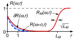
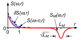
Figure 1: A schematic (not numerically exact) view of the correlation functions $R(\omega,r)$ (top panel) and $S(\omega,r)$ (bottom panel) defined in Eqs. (1) and (2), respectively. The dashed lines denote the $\omega\to 0$ limits [the same function (36) for $R(\omega,r)$ and $S(\omega,r)$]. The shaded regions denote $\delta R(\omega,r)$ and $\delta S(\omega,r)$ as defined in Eq. (4). The features at the Mott length scale $L_{M}$ are denoted by $R_{M}(\omega,r)$ and $S_{M}(\omega,r)$, respectively.

Table 1: Correlation function $R(\omega,r)$ at low frequencies ($\omega\ll 1$).

Model	$R(\omega\to 0,r\gg 1)$	$\delta R(\omega,r\gg 1)$	$R_{M}(\omega,r)$
S1D		$\propto\omega^{2}(L_{M}-3r)e^{2r}$
Q1D-unitary	$\propto r^{-3/2}e^{-r/4}$	$\propto\omega^{2}(L_{M}-3r)^{2}e^{2r}$	$\displaystyle\frac{1}{2}\left(1+{\rm erf}\frac{r-L_{M}}{2\sqrt{r}}\right)$
Q1D-orthogonal		$\propto\omega e^{r/2}$

Table 2: Correlation function $S(\omega,r)$ at low frequencies ($\omega\ll 1$).

Model	$S(\omega\to 0,r\gg 1)$	$\delta S(\omega,r\gg 1)$	$S_{M}(\omega,r)$
S1D		$\propto-\omega^{2}(L_{M}-3r)e^{2r}$
Q1D-unitary	$\propto r^{-3/2}e^{-r/4}$	$\propto-\omega^{2}(L_{M}-3r)^{2}e^{2r}$	$\displaystyle-\frac{1}{2\sqrt{\pi r}}\exp\left[-\frac{(r-L_{M})^{2}}{4r}\right]$
Q1D-orthogonal		$\propto-\omega e^{r/2}$

A more detailed information about localization (in particular, relevant to dynamic properties) can be extracted from correlations between eigenfunctions at different energies. Two such quantities may be defined GDP1 ; GDP2 : the density-of-states (DOS) correlation function,

$$R(\omega,|x_{1}-x_{2}|)=\nu^{-2}\,\Bigl{<}\sum_{n,m}\delta(E_{n}-E)\delta(E_{m}-E-\omega)\\ {}\times|\psi_{n}(x_{1})|^{2}|\psi_{m}(x_{2})|^{2}\Bigr{>}\,,$$ (1)

and the dynamic response function,

$$S(\omega,|x_{1}-x_{2}|)=\nu^{-2}\,\Bigl{<}\sum_{n,m}\delta(E_{n}-E)\delta(E_{m}-E-\omega)\\ {}\times\psi^{*}_{n}(x_{1})\psi_{n}(x_{2})\psi^{*}_{m}(x_{2})\psi_{m}(x_{1})\Bigr{>}\,.$$ (2)

Here the sum is taken over the eigenstates $\psi_{n}$ with energies $E_{n}$, and $\nu$ is the average density of states. The normalization of these correlation functions is chosen in such a way that they are dimensionless quantities with a finite limit in an infinitely long wire. It will be furthermore convenient to measure the lengths in the units of the localization length $\xi$ and the energies in the units of the average level spacing within the localization length $\Delta_{\xi}$ loc-length-definition . With this convention, $R(\omega,r)$ and $S(\omega,r)$ become dimensionless functions of dimensionless parameters.

Both $R(\omega,r)$ and $S(\omega,r)$ were studied analytically in detail in the S1D model GDP1 ; GDP2 , and $R(\omega,r)$ has been recently calculated in the Q1D-unitary model IOS2009 (in all those studies, the weak-disorder limit was assumed). While the limiting form of these correlations at $\omega\to 0$ is determined by the single-wave-function statistics and is therefore universal for both S1D and Q1D models, the corrections at finite $\omega$ distinguish between S1D and Q1D SO07 ; IOS2009 . Qualitatively, the properties of the correlation functions $R(\omega,r)$ and $S(\omega,r)$ in the low-frequency limit $\omega\ll 1$ may be understood using the original argument by Mott about the hybridization of the localized wave functions Mott (the opposite limit $\omega\gg 1$ can be studied by means of the standard perturbation theory). However, the first attempt to promote the Mott’s arguments to quantitative calculations in Ref. SivanImry1987, produced some inaccurate results (as can be seen by comparing to exact expressions GDP1 ), since it neglected mesoscopic fluctuations of the tails of the localized states.

In the present work, we rectify this approach and revisit Mott’s arguments on wave-function hybridization Mott taking into account the log-normal distribution of the tails of the localized states Mirlin-review . Our method is based on a number of assumptions that we introduce in the main text and then explicitly summarize and discuss in the last section of the paper (Section VIII). As a result, we obtain a semi-phenomenological description of the hybridization of the localized states at distances much larger than the localization length, $r\gg 1$. Our theory reproduces correctly the physics at the “Mott length scale”,

$$L_{M}=2\ln(1/\omega),$$ (3)

and the leading correction to $R(\omega,r)$ at $1\ll r<L_{M}$ in the Q1D-unitary model. We further make predictions concerning the properties of $R(\omega,r)$ in the Q1D-orthogonal model and of $S(\omega,r)$ in all the above-mentioned models. These predictions may be checked against future sigma-model calculations in Q1D systems.

II Main results

In the present work, we assume the single-parameter-scaling regime for the tails of the localized states. Namely, we suppose that at distances $r\gg 1$, the decay of the localized wave function may be described by a log-normal distribution with the width and median (or, formally, the variance and the mean of the logarithm) described by one parameter and with an appropriate cut-off of the tails. By combining this assumption with the Mott’s argument about the wave-function hybridization (see subsequent sections for details), we can infer quantitative details about the behavior of the correlation functions (1) and (2) in the low-frequency limit $\omega\ll 1$.

The general structure of those two correlation functions contains two main separate regimes: $r\ll L_{M}$ and $r\sim L_{M}$ (Fig. 1). At $r\ll L_{M}$, the correlations are known to be dominated by the statistics of a single wave function Mott ; SivanImry1987 ; GDP1 ; GDP2 ; IOS2009 , and it is natural to represent them as

$$R(\omega,r)=R(\omega\to 0,r)+\delta R(\omega,r)\,,$$ (4a)

$$S(\omega,r)=S(\omega\to 0,r)+\delta S(\omega,r)\,,$$ (4b)

where $\delta R(\omega,r)$ and $\delta S(\omega,r)$ vanish as $\omega\to 0$.

At $r\sim L_{M}$, the correlation function $R(\omega,r)$ exhibits a crossover from zero to one centered at $L_{M}$ and with a width of the order $\sqrt{L_{M}}$, and the correlation function $S(\omega,r)$ has a negative bump at the same location GDP1 ; GDP2 . The asymptotic form of these features at $\omega\to 0$ will be denoted as $R_{M}(\omega,r)$ and $S_{M}(\omega,r)$, respectively.

Our hybridization argument reproduces the (universal) main asymptotics $R(\omega\to 0,r)$ and $S(\omega\to 0,r)$ at $1\ll r\ll L_{M}$, the (nonuniversal) leading in $\omega$ corrections $\delta R(\omega,r)$ and $\delta S(\omega,r)$, as well as the universal behavior of $R_{M}(\omega,r)$ and $S_{M}(\omega,r)$, see Tables 1 and 2 loc-length-warning . Some of these results can be verified against the existing exact calculations, while others present new conjectures. As a byproduct of our calculation, we also relate the $R(\omega\to 0,r)$ and $S(\omega\to 0,r)$ to the statistics of a single wave function [Eq. (39) below], including the proportionality coefficient.

III Statistics of wave-function tails

We start with a simplified statistical description of a single localized state in terms of the log-normal distribution of its tails. The statistics of a single wave function has been studied in detail in both Q1D and S1D geometries Mirlin-review ; Kolokolov1995 , and we first briefly summarize the existing results and then propose our approximation.

First of all, a localized state $\psi(x)$ can be represented as a product of a slowly varying envelope and a rapidly oscillating short-range component Mirlin-review :

$$\psi(x)=\widetilde{\psi}(x)\cdot\varphi(x)\cdot(A\xi)^{-1/2}$$ (5)

(here we include the dimensional factor $(A\xi)^{-1/2}$, where $A$ is the cross section of the wire, in order to simplify the formulas below). The short-range component $\varphi(x)$ is correlated on the scale of the mean free path $l$ and oscillates on the scale of the particle wave length $\lambda_{F}$. We choose it normalized to $\langle|\varphi(x)|^{2}\rangle=1$. The “envelope” component $\widetilde{\psi}(x)$ is correlated on the scale of the localization length $\xi$ (in S1D, $\xi\sim l$; in Q1D, $\xi\gg l$) and does not oscillate. The two components $\widetilde{\psi}(x)$ and $\varphi(x)$ are distributed independently. It was shown in Refs. Mirlin-review, ; Kolokolov1995, that such a decomposition is exact with the statistics of $\widetilde{\psi}(x)$ being universal for Q1D and S1D systems, and that of $\varphi(x)$ distinguishing between S1D and Q1D and between different symmetry classes in Q1D.

The statistics of $\widetilde{\psi}(x)$ can be most conveniently described in terms of its logarithm

$$\chi(x)=\ln|\widetilde{\psi}(x)|^{2}\,.$$ (6)

As shown in Ref. Mirlin-review, (section 3.2.2), the statistics of $\chi(x)$ is given by a functional integral, which involves a diffusion-type quadratic action in $\chi(x)$ and a delta-function constraint imposing the normalization of the wave function $\int e^{\chi}dx=1$.

An accurate treatment of that functional integral is difficult, and we simplify it by observing that the tails of $\psi(x)$ contribute very little to the normalization, and therefore the normalization-enforcing delta-function term is of little importance for the tails of $\psi(x)$. The normalization is mostly determined by the maxima of $\chi(x)$, and therefore the main role of this delta-term is to normalize the maxima of the function $\chi(x)$. We expect that the distribution of the maxima of $\chi(x)$ has a width of order one and centered around zero.

This suggests our approximation for studying the wave-function tails. Instead of working with a full path integral of Ref. Mirlin-review, , we first fix the position $x_{0}$ and the value $\chi(x_{0})$ of the maximum of $\chi(x)$ (with $|\chi(x_{0})|\lesssim 1$) and replace the normalization constraint by an approximate condition that $\chi(0)<\chi(x_{0})$ everywhere. This guarantees a normalization of the wave function to a “logarithmic” precision: namely, the normalization of wave functions constructed in such a way will be of order one. Furthermore, we will only be interested in a “coarse-grained” behavior of $\chi(x)$: typical scales of interest of $\chi(x)$ will be of order $r$, and therefore for many purposes we do not need to distinguish between the maximum value $\chi(x_{0})$ and zero.

We thus arrive at the following coarse-grained description of the ensemble of the envelopes $\chi(x)$: a localized state is determined by the location $x_{0}$ of its (global) maximum (where $\chi(x_{0})\approx 0$) and the functional measure for the tails (which follows directly from the formula (3.34) of Ref. Mirlin-review, )

$$d\mu_{x_{0}}[\chi(x)]\propto\\ \exp\left(-\int\frac{1}{4}\left[\frac{d\chi}{dx}+{\rm sign}(x-x_{0})\right]^{2}dx\right)\,D\chi(x)$$ (7)

with the constraint $\chi(x)\leq 0$ for all $x$. In particular, the left and right parts of the tails ($x<x_{0}$ and $x>x_{0}$, respectively) are distributed independently. The action (7) describes a diffusion with a drift, and the resulting form of the probability distribution for $\chi(x)$ is approximately normal, with its variance growing linearly with $x$ and its average decreasing linearly with $x$, as $x$ moves away from the center $x_{0}$.

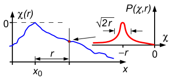
Figure 2: A description of a single-wave-function statistics. The wave function is described by the position $x_{0}$ of its maximum and the distribution of its tails. The one-point probability distribution $P(\chi,r)$ is assumed to have the form (9) at $r\gg 1$.

For our calculations, we will be interested in one- and multi-point probability distributions of $\chi(x)$ for a fixed position of $x_{0}$. Let us start with the one-point probability distribution $P(\chi,r)$, where $r=|x-x_{0}|$. The action (7) results in the differential equation

$$\frac{\partial P}{\partial r}=\frac{\partial^{2}P}{\partial\chi^{2}}+\frac{\partial P}{\partial\chi}$$ (8)

which describes diffusion with a drift. This equation, together with the boundary condition $P(\chi>0)=0$, results in the long-time ($r\gg 1$) asymptotic form of the solution

$$P(\chi,r)=f\left(\frac{\chi}{r}\right)P_{0}(\chi,r)\,,\qquad\chi<0\,,$$ (9)

where

$$P_{0}(\chi,r)=\frac{1}{2\sqrt{\pi r}}\exp\left[-\frac{(\chi+r)^{2}}{4r}\right]$$ (10)

is the normal distribution (Fig. 2). The effect of the boundary condition is the “cut-off” factor $f(\chi/r)$. The exact form of the function $f(z)$ is determined by a short-time evolution (at $r\sim 1$) and is therefore beyond our approximation scheme. The only property that we assume about $f(z)$ (which becomes useful in Section VI) is its asymptotic behavior

$$f(z)\propto-z\quad{\rm at}\quad z\to-0\,.$$ (11)

The normalization of the probability distribution $P(\chi,r)$ implies $f(-1)=1$. Furthermore, the typical values of $\chi(x)$ are not affected by the cut-off factor, and we have a “single-parameter-scaling” relation

$$\frac{1}{2}\langle(\Delta\chi)^{2}\rangle=-\langle\chi\rangle=r\,.$$ (12)

Note that a similar single-parameter scaling is also well-known for the conductance of long wires Abrikosov81 ; Melnikov81 ; Kumar85 ; Shapiro86 .

The above consideration may be directly extended to multi-point probability distributions. For example, consider the probability distribution to find $\chi(x_{1})=\chi_{1}$ and $\chi(x_{2})=\chi_{2}$ under the condition that the maximum of $\chi(x)$ is located at $x_{0}$ (so that $\chi(x_{0})\approx 0$). The form of this probability distribution $P_{x_{0}}(\chi_{1},x_{1};\chi_{2},x_{2})$ depends on the relative positions of $x_{1}$, $x_{2}$, and $x_{0}$ (see Fig. 3). If $x_{1}$ and $x_{2}$ lie on opposite sides of $x_{0}$ (Fig. 3a), then the joint probability distribution factorizes:

$$P_{x_{0}}(\chi_{1},x_{1};\chi_{2},x_{2})=P(\chi_{1},r_{1})P(\chi_{2},r_{2})\,,$$ (13)

where $r_{i}=|x_{i}-x_{0}|$ and $P(\chi,r)$ is given by Eq. (9). In other words, the left and right tails are statistically independent. In the opposite case, if $x_{1}$ and $x_{2}$ belong to the same tail, the distributions of $\chi(x_{1})$ and $\chi(x_{2})$ are correlated. For the configuration shown in Fig. 3b (the point $x_{1}$ lies between $x_{0}$ and $x_{2}$), one gets

$$P_{x_{0}}(\chi_{1},x_{1};\chi_{2},x_{2})=P(\chi_{1},r_{1})P_{0}(\chi_{2}-\chi_{1},r_{2}-r_{1})\,.$$ (14)

Note that the second factor does not involve the cut-off function $f(z)$, since, at $-\chi_{1}\gg 1$ and $-\chi_{2}\gg 1$, the probability of the functional integral (7) to return to $\chi(x)=0$ is exponentially small.

We may note in passing that the two-point distributions (13) and (14) are consistent with the one-point distribution (9). Namely,

$$\int d\chi_{1}\,P_{x_{0}}(\chi_{1},x_{1};\chi_{2},x_{2})=P(\chi_{2},|x_{2}-x_{0}|)\,,$$ (15)

irrespectively of the relative positions of the points $x_{0}$, $x_{1}$, and $x_{2}$.

Generalization of this construction to many-point distributions is straightforward. The only requirements are that the distances between all the points involved exceed the localization length, $|x_{i}-x_{j}|\gg 1$, and that only small tails are considered, $-\chi_{i}\gg 1$.

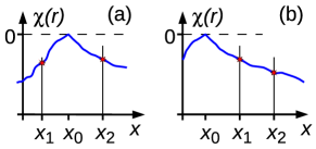
Figure 3: The two-point probability distribution $P_{x_{0}}(\chi_{1},x_{1};\chi_{2},x_{2})$ for a single wave function depends on the ordering of the observation points $x_{1}$, $x_{2}$, and the “center” of the wave function $x_{0}$. (a) For $x_{1}$ and $x_{2}$ belonging to different tails, the distribution factorizes, see Eq. (13). (b) For $x_{1}$ and $x_{2}$ belonging to the same tail, the distribution is given by Eq. (14).

IV Wave-function hybridization

It was realized in the early works on localization that, at $\omega\ll\Delta_{\xi}$, the correlation functions (1) and (2) may be understood in terms of the hybridization of two localized states Mott ; SivanImry1987 . Following the original argument, we may cut the wire into smaller pieces and consider two states $\psi_{A}$ and $\psi_{B}$ localized in different pieces (centered at positions $x_{A}$ and $x_{B}$, respectively, and with energies $E_{A}$ and $E_{B}$). As we connect the pieces of the wire together, the states get hybridized, and such pairs of states give the main contribution to the correlation functions (1) and (2).

To use this argument at a quantitative level, we need to introduce the “hybridization” matrix element $J$ between the states $\psi_{A}$ and $\psi_{B}$. Then the hybridized wave functions are given by the linear combinations

$$\psi_{+}=u_{+}\psi_{A}+u_{-}\psi_{B}\,,\qquad\psi_{-}=u_{-}^{*}\psi_{A}-u_{+}^{*}\psi_{B}\,,$$ (16)

where

$$|u_{\pm}|^{2}=\frac{1}{2}\left(1\mp\frac{\varepsilon}{\Delta}\right)\,,$$ (17)

$\varepsilon=E_{B}-E_{A}$ and

$$\Delta=\sqrt{\varepsilon^{2}+4|J|^{2}}$$ (18)

are the energy splittings before and after hybridization (Fig. 4). Such a pair of hybridized states contributes to the correlation functions (1) and (2), when $\Delta=\omega$.

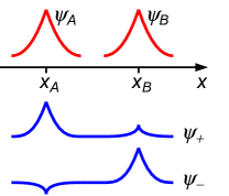
Figure 4: A schematic view of the hybridization of the two localized wave functions $\psi_{A}$ and $\psi_{B}$, as described by Eq. (16).

It turns out that this approximate description reproduces quantitatively many features of the exact results, provided the distribution of the tails (9) is taken into account, and appropriate assumptions on $J$ are made.

Namely, by analogy with the hybridization of states localized in potential wells Landafshits3 , we assume that the hybridization matrix element $J$ is proportional to the product of the two envelopes $\widetilde{\psi}_{A}(x)$ and $\widetilde{\psi}_{B}(x)$:

$$|J|=\Phi\,\widetilde{\psi}_{A}(x)\,\widetilde{\psi}_{B}(x)\,,$$ (19)

where $\Phi$ is a coefficient of order one, which takes into account the short-range oscillations of the wave functions $\psi_{A}(x)$ and $\psi_{B}(x)$. The distribution of $\Phi$ is assumed to be statistically independent of the distributions of the envelopes $\widetilde{\psi}_{A}(x)$ and $\widetilde{\psi}_{B}(x)$. The average $\langle\Phi\rangle$ is taken to be of order one, so that Eq. (19) gives the matrix element $J$ in the units of $\Delta_{\xi}$.

The specific properties of the distribution of $\Phi$ will be of relevance for some of our calculations below. In fact, it is this distribution that distinguishes between the S1D and Q1D geometries and between the different symmetry classes in the Q1D case. Specifically, in Section VII, we will need the behavior of the probability distribution of $\Phi$ at $\Phi\to 0$. Based on an analogy with the random-matrix theory, in that part of the calculation, we will use the following ansatz:

$$dP(\Phi)=\delta(\Phi-\Phi_{0})\,d\Phi\quad{\rm with~{}}\Phi_{0}\sim 1\quad{\rm in~{}S1D}\,,$$ (20a)

$$dP(\Phi)\propto\Phi\,d\Phi\,,\quad\Phi\to 0\quad{\rm in~{}Q1D~{}unitary}\,,$$ (20b)

$$dP(\Phi)\propto d\Phi\,,\quad\Phi\to 0\quad{\rm in~{}Q1D~{}orthogonal}\,.$$ (20c)

Our ansatz for $dP(\Phi)$ in the Q1D-unitary and Q1D-orthogonal cases can be understood in terms of the sum of the hybridization amplitudes over a large number of channels. In the case of the unitary symmetry class, this sum is complex, and therefore its absolute value is distributed as $\Phi\,d\Phi$ at small $\Phi$, while in the orthogonal symmetry class it is real with the measure $d\Phi$ at small $\Phi$.

The wave functions $\widetilde{\psi}_{A}(x)$ and $\widetilde{\psi}_{B}(x)$ in Eq. (19) are taken at some common point $x$ in the tails of the wave functions. One can verify that, due to the log-normal statistics of the tails described in Section III, the probability distribution of the product $\widetilde{\psi}_{A}(x)\widetilde{\psi}_{B}(x)$ is independent of the specific position of the point $x$. In other words, our ansatz (19) gives a consistent definition of the probability distribution of $|J|$. Equivalently, one may also rewrite

$$|J|=\Phi\,e^{\chi_{J}/2}\,,$$ (21)

where the parameter $\chi_{J}$ has a distribution of the type (9), with or without a cut-off factor (depending on the type of the points where the values of $\widetilde{\psi}_{A}(x)$ and $\widetilde{\psi}_{B}(x)$ are fixed).

We are now ready to formulate the improved version of the Mott hybridization argument by combining the three ingredients: (i) the hybridization of the wave functions (16), (ii) the statistical properties of a single wave function (7), and (iii) the properties of the hybridization matrix element (19). To obtain the $\omega\ll\Delta_{\xi}$ limits of the correlation functions (1) and (2), we restrict the sums over $m$ and $n$ to the two hybridized states (16) and arrive at

$$R(\omega,|x_{1}-x_{2}|)=\int dx_{A}\,dx_{B}\int d\mu_{x_{A}}[\chi_{A}(x)]\,d\mu_{x_{B}}[\chi_{B}(x)]\int dP(\Phi)\int d\varepsilon\,|\psi_{+}(x_{1})|^{2}|\psi_{-}(x_{2})|^{2}\,\delta\left(\Delta-\omega\right)\,,$$ (22)

$$S(\omega,|x_{1}-x_{2}|)=\int dx_{A}\,dx_{B}\int d\mu_{x_{A}}[\chi_{A}(x)]\,d\mu_{x_{B}}[\chi_{B}(x)]\int dP(\Phi)\int d\varepsilon\,\psi^{*}_{+}(x_{1})\psi_{+}(x_{2})\psi^{*}_{-}(x_{2})\psi_{-}(x_{1})\,\delta\left(\Delta-\omega\right)\,.$$ (23)

Here the average is taken (i) over the positions of the maxima $x_{A}$ and $x_{B}$ of the envelopes $\widetilde{\psi}_{A}(x)$ and $\widetilde{\psi}_{B}(x)$, respectively; (ii) over the statistical properties of the wave-function tails $d\mu_{x_{A}}[\chi_{A}(x)]$ and $d\mu_{x_{B}}[\chi_{B}(x)]$ defined by Eq. (7), with the constraint $\chi_{\alpha}(x)\leq 0$ [here we define $\chi_{\alpha}(x)=\ln|\widetilde{\psi}_{\alpha}(x)|^{2}$, as in Eq. (6)]; (iii) over the energy difference $\varepsilon$; and (iv) over the coefficient $\Phi$ in Eq. (19).

The following sections are devoted to extracting the three different regimes from the general formalism (22) and (23): the behavior at the Mott scale and the leading and subleading corrections at sub-Mott lengths.

V Behavior at the Mott scale

As pointed out in the early works Mott , the hybridization of localized states introduces the logarithmically large “Mott scale” (3). The leading contribution to the behavior of $R(\omega,r)$ at $r\sim L_{M}$ is obtained by picking out the following term from the general formula (22):

$$|\psi_{+}(x_{1})|^{2}|\psi_{-}(x_{2})|^{2}\longrightarrow|u_{+}|^{4}|\psi_{A}(x_{1})|^{2}|\psi_{B}(x_{2})|^{2}\,.$$ (24)

Since the wave functions $\psi_{A}$ and $\psi_{B}$ are localized at distances of order one, and $R(\omega,r)$ at $r\sim L_{M}$ varies at a logarithmically larger scale ($\delta r\sim\sqrt{L_{M}}$, as shown below), the variables $x_{A}$ and $x_{B}$ are nearly pinned to the points $x_{1}$ and $x_{2}$, respectively. Then integration over $x_{A}$ and $x_{B}$ yields just the unit normalization of $\psi_{A}$ and $\psi_{B}$, and we get

$$R_{M}(\omega,r)=\int dP(J)\int d\varepsilon\,\delta(\Delta-\omega)|u_{+}|^{4}\,,$$ (25)

where $\Delta$ and $u_{+}$ are functions of $\varepsilon$ and $J$ defined by Eqs. (17) and (18). The measure of integration over $J$ is

$$dP(J)=f^{2}\left(\frac{\chi_{J}}{r}\right)\,P_{0}(\chi_{J},r)\,d\chi_{J}\,dP(\Phi),$$ (26)

where $J$ is parameterized by Eq. (21), $P_{0}(\chi_{J},r)$ is the normal distribution (10), and $f(\chi_{J}/r)$ is the cut-off function [the same as in Eq. (9)]. The integral over $\varepsilon$ may be easily taken, which gives

$$R_{M}(\omega,r)=\int dP(J)\,\frac{1}{2}\left(\frac{\varepsilon}{\omega}+\frac{\omega}{\varepsilon}\right)\,,$$ (27)

where $\varepsilon=\sqrt{\omega^{2}-4|J|^{2}}$.

Since the main contribution to the integral comes from logarithmically large intervals of $\chi_{J}$, one can approximate

$$\frac{1}{2}\left(\frac{\varepsilon}{\omega}+\frac{\omega}{\varepsilon}\right)\approx\theta\left(\omega-2|J|\right)$$ (28)

in Eq. (27) [the step function in the right-hand side takes care of the integration limits] and disregard the exact form of the distribution of $\Phi$. Then, within these approximations, one gets

$$R_{M}(\omega,r)\approx\int_{-\infty}^{2\ln\omega}f^{2}\left(\frac{\chi_{J}}{r}\right)\,P_{0}(\chi_{J},r)\,d\chi_{J}\\ =\frac{1}{2}\left[1+{\rm erf}\left(\frac{r-L_{M}}{2\sqrt{r}}\right)\right]\,,$$ (29)

i.e., the result reported in the last column of Table 1. Note that the cut-off function $f(\chi_{J}/r)$ does not play any role in this calculation, since $f(-1)=1$ by the normalization of probability.

We can further repeat the same procedure for the correlation function $S(\omega,r)$ given by Eq. (23) by selecting the term

$$\psi^{*}_{+}(x_{1})\psi_{+}(x_{2})\psi^{*}_{-}(x_{2})\psi_{-}(x_{1})\\ \longrightarrow-|u_{+}|^{2}|u_{-}|^{2}|\psi_{A}(x_{1})|^{2}|\psi_{B}(x_{2})|^{2}\,.$$ (30)

We then arrive at the formula similar to Eq. (25), but with $|u_{+}|^{4}$ replaced by $-|u_{+}|^{2}|u_{-}|^{2}$. The formula (27) then gets replaced by

$$S_{M}(\omega,r)=\int dP(J)\,\frac{1}{2}\left(\frac{\varepsilon}{\omega}-\frac{\omega}{\varepsilon}\right)\,.$$ (31)

Now we cannot simply replace $\varepsilon$ by $\omega$, but need to expand to the next order. In fact, we can re-express

$$\frac{1}{2}\left(\frac{\varepsilon}{\omega}-\frac{\omega}{\varepsilon}\right)=\frac{\partial}{\partial\chi_{J}}\frac{\varepsilon}{\omega}\approx-\delta\left(\chi_{J}-2\ln\frac{\omega}{2\Phi}\right)\,,$$ (32)

which allows us to integrate over $\chi_{J}$ to obtain

$$S_{M}(\omega,r)\approx-\frac{1}{2\sqrt{\pi r}}\exp\left[-\frac{(r-L_{M})^{2}}{4r}\right]\,,$$ (33)

again independently of the distribution of $\Phi$ and therefore universally valid in S1D and Q1D systems (including the numerical prefactor loc-length-warning ).

The result (29) has been previously rigorously derived in S1D and in Q1D-unitary cases GDP1 ; IOS2009 , and the result (33) in the S1D case GDP2 . Note that the location and width of the features in $R_{M}(\omega,r)$ and $S_{M}(\omega,r)$ reflect directly the median and the width of the log-normal distribution for $\chi_{J}$ in Eq. (21). In our ansatz (10), we take them related to each other, which corresponds to the single-parameter-scaling regime ATAF80 ; Melnikov81 ; Kumar85 ; Shapiro86 . In Ref. SivanImry1987, , a qualitative behavior of $R(\omega,r)$ at the Mott scale was also explained from the hybridization arguments, but the correct quantitative expression (29) could not be obtained without taking into account the log-normal distribution of the wave-function tails.

VI Leading order at distances much shorter than the Mott scale

At distances $1\ll r\ll L_{M}$, the correlation functions $R(\omega,r)$ and $S(\omega,r)$ can be found, to the leading order, from the general expressions (22) and (23) if one retains only the contributions from $\psi_{A}$ in both $\psi_{+}$ and $\psi_{-}$:

$$\!\!\!\!\!\!|\psi_{+}(x_{1})|^{2}|\psi_{-}(x_{2})|^{2}\quad\text{and}\quad\psi^{*}_{+}(x_{1})\psi_{+}(x_{2})\psi^{*}_{-}(x_{2})\psi_{-}(x_{1})\,\\ \longrightarrow|u_{+}|^{2}|u_{-}|^{2}|\psi_{A}(x_{1})|^{2}|\psi_{A}(x_{2})|^{2}\,.$$ (34)

Then, using the relation (32), we can integrate over all the variables, except for $x_{A}$ and $\chi_{A}$ (in the order $\varepsilon$, $\chi_{J}$, $x_{B}$, $\Phi$) and arrive at the result

$$R(\omega,r)\approx S(\omega,r)\\ \approx 2\int dx_{A}\,d\mu_{x_{A}}[\chi_{A}(x)]\,|\psi_{A}(0)|^{2}|\psi_{A}(r)|^{2}\,.$$ (35)

Thus the short-distance behavior of these correlation functions is universal for S1D and Q1D models and is only determined by the single-wave-function statistics. This result was rigorously derived for S1D (as follows from Refs. Gogolin, , GDP1, , and GDP2, ) and Q1D-unitary cases IOS2009 , and the exact form of this function is known,

$$R(\omega\to 0,r)=4\pi^{2}\frac{\partial^{2}}{\partial r^{2}}\int_{0}^{\infty}k\,dk\,\frac{\tanh\pi k}{\cosh^{2}\pi k}e^{-(k^{2}+1/4)r}\,.$$ (36)

Within our approximate method, we cannot derive this exact expression, but we can access its $r\gg 1$ limit. In this case, the main contribution comes from $x_{A}$ located between $0$ and $r$ (see Fig. 3a), with the two tails of the wave function $\psi_{A}$ distributed independently, according to Eq. (13):

$$R(\omega,r)\approx S(\omega,r)\approx\int_{0}^{r}dx_{A}\int_{-\infty}^{0}d\chi_{1}\int_{-\infty}^{0}d\chi_{2}\\ {}\times P(\chi_{1},x_{A})P(\chi_{2},r-x_{A})e^{\chi_{1}+\chi_{2}}\,.$$ (37)

If we use our ansatz (9) for $P(\chi,r)$, then this integral formally diverges at $x_{A}\to 0$ and $x_{A}\to r$. This means that the main contribution to the correlation functions comes from configurations where the maximum of the wave functions coincides (within the localization length) with one of the two points. At such short distances, our ansatz (9) is not applicable, but we can estimate the correlation function, up to a numerical prefactor, by cutting off the integral in $x_{A}$ within a localization length from $0$ and $r$ [i.e., by integrating over $x_{A}$ in the limits $(\delta,r-\delta)$ with $\delta\sim 1$]. This immediately leads us to the asymptotic expression (at $r\gg 1$)

$$R(\omega,r)\approx S(\omega,r)\propto r^{-3/2}e^{-r/4}\,,$$ (38)

where the proportionality coefficient cannot be calculated within our approximation.

The asymptotic expression (38) is in agreement with the exact expression (36) Gogolin ; Kolokolov1995 ; Mirlin-review ; IOS2009 . Note that the form of the cut-off in the probability distribution (9) was important for calculating the correct power in the pre-exponent in Eq. (38). In fact, the correlation functions $R(\omega\to 0,r)$ and $S(\omega\to 0,r)$ are dominated not by “typical” localized wave functions, but by the rare events, when the wave function $\psi_{A}$ has two peaks at the positions $0$ and $r$ of comparable height. This can also be seen from the exponential decay $e^{-r/4}$, which does not describe the decay of a “typical” wave function [whose weight decays as $e^{-r}$, according to Eq. (12)], but is four times slower.

Somewhat similar rare events are important for the statistics of wave functions in the metallic limit AKL , which also results in log-normal tails. However, the metallic regime is beyond the scope of the present paper.

Note that the derivation of the relation (35) does not use the condition $r\gg 1$ (which is only needed for calculating its right-hand side), and is therefore valid for any $r$ (in the limit $\omega\to 0$). In terms of wave-function correlations, we may also rewrite Eq. (35) as

$$R(\omega\to 0,|x_{1}-x_{2}|)=S(\omega\to 0,|x_{1}-x_{2}|)\\ =2\xi\,\nu^{-1}\sum_{n}\delta(E_{n}-E)|\psi_{n}(x_{1})|^{2}|\psi_{n}(x_{2})|^{2}\,,$$ (39)

(in this equation, we restore the physical units). This relation (without specifying the numerical prefactor) was already proposed in Ref. SivanImry1987, based on similar hybridization arguments. However, the approach used in that work could not correctly reproduce the asymptotic behavior (38), since it did not include the log-normal distribution of the wave-function tails crucial for such a calculation.

VII Subleading order at distances much shorter than the Mott scale

Remarkably, we can extend our method further to finding non-universal corrections $\delta R(\omega,r)$ and $\delta S(\omega,r)$ [defined in Eqs. (4)] to the asymptotic behavior (38). Such corrections are given by the same “cross-terms” (24) and (30), as in the calculations of $R_{M}(\omega,r)$ and $S_{M}(\omega,r)$ in Section V. One can check that, for this term, the main contribution comes from configurations with the points $x_{A}$ and $x_{B}$ (the maxima of the wave functions $\psi_{A}$ and $\psi_{B}$) located outside the interval $(x_{1},x_{2})$, see Fig. 5.

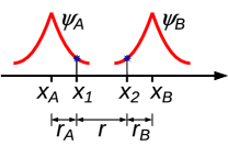
Figure 5: An illustration of notation for the calculation of the subleading order at $1\ll r\ll L_{M}$. The centers $x_{A}$ and $x_{B}$ of the pair of localized states are located outside the interval $(x_{1},x_{2})$. The variables $r_{A}$, $r_{B}$, and $r$ used in Eq. (41) are the pairwise distances between the four points $x_{A}$, $x_{1}$, $x_{2}$, and $x_{B}$.

For calculating $\delta R(\omega,r)$, we start with the general expression (22), where we only keep the term (24). Unlike in the calculation of Section V, here the tails of the wave functions contribute, and therefore we need to take into account their log-normal distributions. If we write $|\psi_{A}(x_{1})|^{2}=e^{\chi_{A}}$ and $|\psi_{B}(x_{2})|^{2}=e^{\chi_{B}}$, then the hybridization matrix element $|J|$ may be expressed in the form (21) with

$$\chi_{J}=\chi_{A}+\chi_{B}+\chi.$$ (40)

Here $\chi_{A}$, and $\chi_{B}$ are distributed with the probability distribution (9) (with the cut-off) and the distribution of $\chi$ is given by Eq. (10) (without the cut-off) [compare with an analogous form of Eq. (14)]. In the calculations of this section, we further neglect the cutoffs, since all the three parameters $-\chi$, $-\chi_{A}$, and $-\chi_{B}$ are much larger than one and the integrals with respect to them can be done at the saddle-point level. The cut-off functions contribute only to the overall numerical coefficient, which is beyond the precision of our calculation.

After integrating Eq. (22) over $\varepsilon$, we arrive at

$$\delta R(\omega,r)\propto\int_{0}^{\infty}dr_{A}\int_{0}^{\infty}dr_{B}\int_{-\infty}^{0}d\chi_{A}\int_{-\infty}^{0}d\chi_{B}\\ {}\times P_{0}(\chi_{A},r_{A})P_{0}(\chi_{B},r_{B})e^{\chi_{A}+\chi_{B}}\\ {}\times\int d\chi\,P_{0}(\chi,r)\int dP(\Phi)\,\frac{1}{2}\left(\frac{\varepsilon}{\omega}+\frac{\omega}{\varepsilon}\right)\,.$$ (41)

Like in the calculation in Section V, we can use the approximation (28). Furthermore, the integrals over $r_{A}$ and $r_{B}$ can be calculated at the saddle-point level (thereby fixing $r_{A}=-\chi_{A}$ and $r_{B}=-\chi_{B}$), and afterwards we integrate over $\chi_{A}$ and $\chi_{B}$. The resulting expression is

$$\delta R(\omega,r)\propto\int dP(\Phi)\int\frac{d\chi}{2\sqrt{\pi r}}\exp\left[-\frac{(\chi+r)^{2}}{4r}\right]\\ \times(z+1)e^{-z}\Big{|}_{z=\max(0,\chi-2\ln\frac{\omega}{2\Phi})}\,.$$ (42)

One can show that, at $r<L_{M}/3$, the main contribution comes from the region $\chi-2\ln\frac{\omega}{2\Phi}>0$. The integral in $\chi$ can be done in the saddle-point approximation, which sets $\chi=-3r$. Finally, only the integral over $\Phi$ remains [at our level of approximation, we also neglect $+1$ in the second line of Eq. (42)]:

$$\delta R(\omega,r)\propto\omega^{2}e^{2r}\int_{\Phi_{\omega}}^{\sim 1}dP(\Phi)\,\frac{\ln\Phi-\ln\Phi_{\omega}}{\Phi^{2}}\,,$$ (43)

where $\Phi_{\omega}=\exp\left[-(L_{M}-3r)/2\right]$. Estimating the integral (43) with the distributions $dP(\Phi)$ given by Eqs. (20) yields the results reported in the middle column of Table 1.

An analogous calculation can also be performed for $\delta S(\omega,r)$ starting with Eq. (23). The calculation parallels the one above, with the only difference that $(1/2)(\varepsilon/\omega+\omega/\varepsilon)$ in Eq. (41) must be replaced by

$$\frac{1}{2}\left(\frac{\varepsilon}{\omega}-\frac{\omega}{\varepsilon}\right)\approx-\delta\left(2\ln\frac{\omega}{2\Phi}-\chi-\chi_{A}-\chi_{B}\right)\,.$$ (44)

This results in

$$\delta S(\omega,r)\propto-\int dP(\Phi)\int\frac{d\chi}{2\sqrt{\pi r}}\exp\left[-\frac{(\chi+r)^{2}}{4r}\right]\\ \times ze^{-z}\Big{|}_{z=\max(0,\chi-2\ln\frac{\omega}{2\Phi})}\,.$$ (45)

To the precision of our approximation, this expression is opposite in sign to Eq. (42). Therefore, we conclude that, within our approximation, $\delta S(\omega,r)\approx-\delta R(\omega,r)$. The corresponding formulas are reported in the middle column of Table 2. Note that our method does not give the numerical coefficients in $\delta R(\omega,r)$ and $\delta S(\omega,r)$, but predicts that they have the same absolute value and are opposite in sign [positive for $\delta R(\omega,r)$ and negative for $\delta S(\omega,r)$].

One can compare our results of this section with the exact calculations. The only case, where a direct comparison is possible is the Q1D-unitary case, where $\delta R(\omega,r)$ was computed in Ref. IOS2009, and, to the leading order, coincides (up to a numerical prefactor) with our present result. Note that our results for $\delta R(\omega,r)$ and $\delta S(\omega,r)$ in the S1D and Q1D-uintary cases are only applicable at $r<L_{M}/3$. The new length $L_{M}/3$ appeared in Ref. IOS2009, as the distance at which the correction $\delta R(\omega,r)$ in the Q1D-uintary case changes its asymptotic form (in technical terms, there was a switching of the pole and the saddle in the integral determining the leading form of the correction).

Another situation where an indirect comparison can be made is the S1D case. There, using the formalism of Ref. GDP1, , one can show SO07 that $\delta R(\omega,r)$, at small $r$ starts with the order $\omega^{2}\ln\omega$, i.e. consistent with our result for the S1D case (strictly speaking, the comparison is not accurate, since our result is only applicable at $r\gg 1$ while the expansion of the result from Ref. GDP1, is done at $r\ll 1$ but we expect that the leading $\omega$ dependence is the same in both regimes). In the other cases, there are no exact calculations to which our results reported in Tables 1 and 2 could be compared, thus they should be considered as conjectures.

VIII Summary, discussion, and outlook

To summarize, in this paper we propose a simple technique of treating correlation of wave functions in Anderson localization in terms of hybridization of localized states. While the essence of our method repeats the well-known Mott argument, supplementing it with a log-normal probability distribution for the tails of localized wave functions (and, consequently, for the hybridization matrix elements) gives the method a quantitative power. We have checked that the results produced with our simplified method reproduce quantitatively the main features of the available exact results (obtained by more sophisticated techniques).

Nevertheless, we should emphasize that the presented method remains a phenomenological recipe, and its justification still needs to be completed. The method depends on several assumptions of various level of rigor. For the benefit of the reader, we list them below:

• A possibility to define localized wave functions that are further hybridized into the eigenstates (16) close in energy. These wave functions $\psi_{A}$ and $\psi_{B}$ are not rigorously defined in our argument, and the formalization of this step would be helpful for a rigorous justification of the method.

• The log-normal distribution of the wave-function tails (10), supplemented by a suitable cutoff (9). While we present some arguments in favor of these formulas, they are not formally derived. We hope that a rigorous derivation of this step may be possible with the methods of Ref. Mirlin-review, .

• The hybridization matrix elements (21) are assumed to be proportional to $\widetilde{\psi}_{A}(x)\widetilde{\psi}_{B}(x)$, the product of the two hybridizing tails, and therefore to obey the same log-normal distribution. Since neither $J$ nor $\psi_{A,B}$ are formally defined, this assumption also remains a phenomenological construction.

• The factor $\Phi$ in (21) reflecting the interference of channels. Its probability distributions (20) are introduced phenomenologically.

Note that, for different calculations, different assumptions play a role. At the Mott length scale (Section V), we only used the assumptions 1 and 3, with the assumptions 2 and 4 being irrelevant. For the leading behavior at $1\ll r\ll L_{M}$ (Section VI), we also used the assumption 2, while in Section VII we additionally need the assumption 4 to calculate the subleading terms $\delta R(\omega,r)$ and $\delta S(\omega,r)$.

We wish to remark here that our method was developed under the specific assumption of a weak disorder (specifically, it is applicable in the model of the Gaussian white noise), which implies the single-parameter-scaling relation (12) between the variance and the average of the wave-function tail. However, the method can be extended to other interesting models of localization by relaxing this assumption. This would imply a modification of the log-normal probability distributions (9) and (10) in the assumptions 2 and 3. One example where such a modification may be applicable is localization far below the mobility edge (see, e.g., Refs. HSW80, ; KLP03, ; Gruzberg, ). Another interesting example is the exactly solvable localization problem with the Cauchy-distributed disorder considered in Ref. DLA00, . In that model, the single-parameter-scaling relation (12) does apply, but with a different coefficient. We believe that such a system can also be treated by our method with a suitably modified probability distributions (9) and (10).

Finally, it would be interesting to extend our approach to higher dimensions. The key issue for such an extension is the log-normal distribution of the wave-function tails (our assumption 2 above). While we are not aware of such results for wave functions in higher-dimensions, a similar claim was made for the probability distribution of the conductance Shapiro86 . Namely, it was shown that, in the weak-scattering case and in the insulating phase, the conductance distribution in the large-system-size limit is log-normal with the single-parameter-scaling relation between the average and the variance of the form (12). Therefore one may assume that a similar universal distribution is also valid for the wave-function tails. If it is indeed the case, then our calculations in Sections V and VI can be straightforwardly extended to higher dimensions. In particular, the counterpart of Eq. (39) in any dimension would read

$$R(\omega\to 0,|x_{1}-x_{2}|)=S(\omega\to 0,|x_{1}-x_{2}|)\\ =S_{d-1}L_{M}^{d-1}\xi\,\nu^{-1}\sum_{n}\delta(E_{n}-E)|\psi_{n}(x_{1})|^{2}|\psi_{n}(x_{2})|^{2}\,,$$ (46)

where $S_{d-1}$ is the area of the $(d-1)$-dimensional sphere (e.g., in our one-dimensional case, $S_{0}=2$), and the definition (3) of $L_{M}$ remains the same in any dimension. Also, under the same conditions, the behavior of $R_{M}(\omega,r)$ and $S_{M}(\omega,r)$ (the right column of Tables 1 and 2 calculated in Section V) would be universal in any dimension. This implies, in particular, the validity of the Mott formula for the frequency-dependent conductivity $\sigma(\omega)\propto\omega^{2}(\ln\omega)^{d+1}$ in any dimension (which can be deduced from $S_{M}(\omega,r)$, see, e.g., Ref. GDP2, ), in agreement with the original argument Mott .

- (1) P. W. Anderson, Phys. Rev. 109, 1492 (1958).
- (2) P. A. Lee, T. V. Ramakrishnan, Rev. Mod. Phys. 57, 287 (1985).
- (3) B. Kramer and A. MacKinnon, Rep. Prog. Phys. 56, 1469 (1993).
- (4) N. F. Mott and W. D. Twose, Adv. Phys. 10, 107 (1961).
- (5) M. E. Gertsenshtein and V. B. Vasil’ev, Teor. Veroyatn. Primen. 4, 424 (1959); ibid. 5, 3(E) (1959) [Theor. Probab. Appl. 4, 391 (1959); ibid. 5, 340(E) (1959)].
- (6) D. J. Thouless, Phys. Rev. Lett. 39, 1167 (1977).
- (7) O. N. Dorokhov, Pis’ma v Zh. Eksp. Teor. Fiz. 36, 259 (1982) [Sov. Phys. JETP Lett. 36, 318 (1982)].
- (8) C. W. J. Beenakker, Rev. Mod. Phys. 69, 731 (1997).
- (9) A. D. Mirlin, Phys. Rep. 326, 259 (2000).
- (10) V. L. Berezinsky, Zh. Eksp. Teor. Fiz. 65, 1251 (1973) [Sov. Phys. JETP 38, 620 (1974)].
- (11) V. L. Berezinsky and L. P. Gor’kov, Zh. Eksp. Teor. Fiz. 77, 2498 (1979) [Sov. Phys. JETP 50, 1209 (1979)].
- (12) A. Ossipov and V. E. Kravtsov, Phys. Rev. B 73, 033105 (2006).
- (13) V. E. Kravtsov and V. I. Yudson, Ann. Phys. 326, 1672 (2011).
- (14) K. B. Efetov, Adv. Phys. 32, 53 (1983).
- (15) K. B. Efetov and A. I. Larkin, Zh. Eksp. Teor. Fiz. 85, 764 (1983) [Sov. Phys. JETP 58, 444 (1983)].
- (16) K. B. Efetov, Supersymmetry in Disorder and Chaos (Cambridge University Press, New York, 1997).
- (17) M. L. Mehta, Random Matrices (Academic Press, Boston, 1991).
- (18) A. D. Mirlin, J. Math. Phys. 38, 1888 (1997).
- (19) A. A. Gogolin, V. I. Mel’nikov, and E. I. Rashba, Zh. Eksp. Teor. Fiz. 69, 328 (1975) [Sov. Phys. JETP 42, 168 (1975)]; A. A. Gogolin, Zh. Eksp. Teor. Fiz. 71, 1912 (1976) [Sov. Phys. JETP 44, 1003 (1976)].
- (20) I. M. Lifshits, S. A. Gredeskul, and L. A. Pastur, Introduction to the theory of disordered systems (Wiley, New York, 1988).
- (21) I. V. Kolokolov, Physica D 86, 134 (1995).
- (22) E. Abrahams, P. W. Anderson, D. C. Licciardello, and T. V. Ramakrishnan, Phys. Rev. Lett. 42, 673 (1979).
- (23) P. W. Anderson, D. J. Thouless, E. Abrahams, and D. S. Fisher, Phys. Rev. B 22, 3519 (1980).
- (24) B. Shapiro, Phys. Rev. B 34, 4394 (1986); Philos. Mag. B 56, 1031 (1987).
- (25) A. Cohen, Y. Roth, and B. Shapiro, Phys. Rev. B 38, 12125 (1988)
- (26) L. I. Deych, A. A. Lisyansky, and B. L. Altshuler, Phys. Rev. Lett. 84, 2678 (2000); Phys. Rev. B 64, 224202 (2001).
- (27) L. P. Gor’kov, O. N. Dorokhov, and F. V. Prigara, Zh. Eksp. Teor. Fiz. 84, 1440 (1983) [Sov. Phys. JETP 57, 838 (1983)]
- (28) L. P. Gor’kov, O. N. Dorokhov, and F. V. Prigara, Zh. Eksp. Teor. Fiz. 85, 1470 (1983) [Sov. Phys. JETP 58, 852 (1983)]
- (29) In Q1D wires, the localization length can be microscopically expressed as EL83 ; Efetov-book , where is the density of states, is the cross section of the wire, is the diffusion coefficient, and is the level-repulsion parameter ( in the Q1D-orthogonal case and in the Q1D-unitary case). We define the localization energy spacing in all cases as .
- (30) D. A. Ivanov, P. M. Ostrovsky, and M. A. Skvortsov, Phys. Rev. B 79, 205108 (2009).
- (31) M. A. Skvortsov and P. M. Ostrovsky, Pis’ma v ZhETF 85, 79 (2007) [JETP Lett. 85, 72 (2007)].
- (32) N. F. Mott, Philos. Mag. 17, 1259 (1968); 22, 7 (1970).
- (33) U. Sivan and Y. Imry, Phys. Rev. B 35, 6074 (1987).
- (34) Note that since enters the expression for the localization length loc-length-definition , the “universality” of some of our formulas only means that they have the same form when expressed in terms of the corresponding and not in any case invariance with respect to time-reversal-symmetry-breaking perturbations.
- (35) A. A. Abrikosov, Solid State Communic. 37, 997 (1981).
- (36) V. I. Mel’nikov, Fiz. Tverd. Tela (Leningrad) 23, 782 (1981) [Sov. Phys. Solid State 23, 444 (1981)].
- (37) N. Kumar, Phys. Rev. B 31, 5513 (1985).
- (38) L. D. Landau and E. M. Lifshitz, Quantum Mechanics: Non-Relativistic Theory (Pergamon Press, 1985).
- (39) B. L. Altshuler, V. E. Kravtsov, and I. V. Lerner, Distribution of mesoscopic fluctuations and relaxation processes in disordered conductors, in Mesoscopic phenomena in solids, eds. B. L. Altshuler, P. A. Lee, and R. A. Webb, Elsevier (1991).
- (40) A. Houghton, L. Schäfer, and F. J. Wegner, Phys. Rev. B 22, 3598 (1980).
- (41) W. Kirsch, O. Lenoble, and L. Pastur, J. Phys. A: Math. Gen. 36, 12157 (2003).
- (42) I. Gruzberg, unpublished.