Phase separation in low-density neutron matter

Abstract

Low-density neutron matter has been studied extensively for many decades, with a view to better understanding the properties of neutron-star crusts and neutron-rich nuclei. Neutron matter is beyond experimental control, but in the past decade it has become possible to create systems of fermionic ultracold atomic gases in a regime close to low-density neutron matter. In both these contexts pairing is significant, making simple perturbative approaches impossible to apply and necessitating ab initio microscopic simulations. Atomic experiments have also probed polarized matter. In this work, we study population-imbalanced neutron matter (possibly relevant to magnetars and to density functionals of nuclei) arriving at the lowest-energy configuration to date. For small to intermediate relative fractions the system turns out to be fully normal, while beyond a critical polarization we find phase coexistence between a partially polarized normal neutron gas and a balanced superfluid gas. As in cold atoms, a homogeneous polarized superfluid is close to stability but not stable with respect to phase separation. We also study the dependence of the critical polarization on the density.

I Introduction

The phase structure of polarized (or population-imbalanced) Fermi gases is very rich. The energetically favored phase depends on the masses and relative populations of the species, the interaction strength, and whether the interactions are long ranged. Polarized gases can exist in a variety of physical systems, including ultracold trapped atomic Fermi gases Giorgini:2008 , dense hadronic phases near the cores of neutron stars Fantoni:2001 ; Vidana:2002 ; Rios:2005 , and possibly quark matter Alford:1999pa .

In this paper we focus on the possibility that neutrons in the inner crust of neutron stars are spin-polarized Gezerlis:2011 . Theoretical calculations suggest that this region, which is about a kilometer thick, features unbound neutrons while the protons cluster in neutron rich nuclei. While interactions with nuclei affect the properties of the unbound neutrons Pethick:2010zf ; Cirigliano:2011 , in this work we consider an isolated neutron fluid and compute the conditions for the coexistence of an unpolarized phase and a polarized phase at densities roughly $30-250$ times smaller than the nuclear saturation density. A polarized phase in the neutron star crust will have a larger specific heat and therefore its presence may affect the time scales associated with observed crustal transient phenomena Brown:2009 . Neutron superfluidity also affects thermal transport properties Aguilera:2009 ; Alford:2011 . If the polarization is large enough all effects of superfluidity are expected to disappear.

At the low densities we consider, the dominant term in the interaction between spin-up and spin-down neutrons is an $s$-wave potential with a scattering length $a\sim-18.6$ fm and range $r_{e}\sim 2.7$ fm. In a balanced system this attraction drives the formation of Cooper pairs of spin-up and spin-down neutrons of opposite momenta resulting in a neutron superfluid whose properties can be understood qualitatively using BCS theory. All the neutrons are paired and the number of up and down species is equal. Even at densities much smaller than the nuclear saturation density, $a$ is much larger than the interparticle spacing and obtaining quantitatively reliable results requires non-perturbative techniques. Detailed Quantum Monte Carlo (QMC) simulations have calculated the energy density ${\cal{E}}$ up to densities equal to or larger than the nuclear saturation density Carlson:Morales:2003 ; Gezerlis:2008 . At low densities, the $s$-wave pairing gap obtained peaks at nearly $2$ MeV.

Magnetic fields tend to split the up and down Fermi surfaces thus disrupting the pairing and creating a polarization. For magnetic fields ($B$) smaller than $10^{16}-10^{17}$ Gauss, pairing wins (assuming no effect coming from the lattice of nuclei), while larger fields can create a polarized phase. In BCS theory, the critical field, or the resulting chemical potential split ($\delta\mu=g_{N}\mu_{N}B$ where $g_{N}\mu_{N}$ is the neutron magnetic moment), is called the Clogston-Chandrasekhar point. At this point, the BCS superfluid can coexist in equilibrium with a partially polarized normal phase which is essentially a gas of free neutrons. Numerically $\delta\mu_{c}=\Delta/\sqrt{2}$ where $\Delta$ is the gap in the BCS phase. A weakly polarized gas of neutrons confined in a volume forms a mixed phase Bedaque:2003 consisting of the BCS and normal phases with volume fractions depending on the polarization. Hartree corrections substantially modify the Clogston-Chandrasekhar point even for modest couplings $|k_{F}a|\sim 0.5$, where $k_{F}=(3\pi^{2}n)^{1/3}$ is the Fermi wave vector Sharma:2008rc .

At strong coupling (mathematically given by $|k_{F}a|\gtrsim 1$) the energies of both the superfluid and the normal phase need to be computed non-perturbatively. In this paper, we perform these calculations for the normal phase and find the critical polarization at which it can coexist with the superfluid phase. We also compare the energy of a phase separated state with the previously evaluated Gezerlis:2011 homogeneous polarized superfluid phase. In this paper we only consider competition between homogeneous and isotropic phases and ignore the possibility of promising but still unconfirmed scenarios (like $p-$wave Bulgac:2006 and inhomogeneous phases Bulgac:2008 ).

As mentioned above, our microscopic ab initio calculations may impact the observed behavior of neutron stars with extremely large internal magnetic fields. It is interesting to concurrently examine possible connections of such simulations with terrestrial experiments. Our results may be useful for constraining Density Functional Theories (DFTs) that are employed to study properties of heavy nuclei. Equation of state results at densities close to the nuclear saturation density have been used for some time to constrain Skyrme and other other density functional approaches to heavy nuclei Bender:2003 . The potential significance of such calculations has led to a series of publications on the equation of state of low-density neutron matter over the last few decades Friedman:1981 ; Akmal:1998 ; Carlson:Morales:2003 ; Schwenk:2005 ; Margueron:2007b ; Baldo:2008 ; Epelbaum:2008b ; Epelbaum:2008a ; Abe:2009 ; Gandolfi:2009 ; Rios:2009 ; Hebeler:2010 . The density-dependence of the ${}^{1}S_{0}$ gap in low-density neutron matter has also been used to constrain Skyrme-Hartree-Fock-Bogoliubov treatments in their description of neutron-rich nuclei Chamel:2008 . Similarly, an ongoing project is studying the limit of extreme polarization in neutron matter Forbes:2011b . This limit is known in condensed-matter physics as the “polaron” problem: one impurity embedded in a sea of fermions. Quantities of interest here include the polaron binding energy and its effective mass, which can be used to constrain Skyrme and other functionals. In this line of study, DFTs can be constrained by the equation of state of polarized unpaired neutron matter that we report here.

Another connection of our calculations with experiment may be possible through the field of atomic ultracold Fermi gases. There, the scattering length of the interaction between two hyperfine states near a Feshbach resonance can be tuned by changing the magnetic field. Most experiments have been performed in the region where the scattering length is infinite (unitarity limit) and the effective range is negligible Luo:2009 ; Navon:2010 ; Carlson:2008 ; Schirotzek:2008 ; Shin:2008 . QMC calculations performed with the same techniques that we use here in the same limit give results that agree well with the experiments for both unpolarized Carlson:2003 ; Astrakharchik:2004 ; Gezerlis:2008 and polarized Carlson:2005 ; Lobo:2006 ; Pilati:2008 ; Gezerlis:2009 Fermi gases and this gives us confidence in applying the same techniques to the problem with finite $a$ and $r_{e}$. More directly, by tuning the scattering length and the effective range Marcelis:2008 it may be possible to obtain a system with similar values of $k_{F}a$ and $k_{F}r_{e}$ as the inner crust and test our results.

II Construction of the mixed phase

The conditions for a polarized phase ($P$) to be in phase equilibrium with an unpolarized superfluid ($SF$) phase are as follows:

1. The pressures of the two phases should be equal.

2. The average chemical potential of the two species in the phases, $\mu=(\mu_{a}+\mu_{b})/2$, should be equal.

3. The chemical potential splitting, $\delta\mu=(\mu_{a}-\mu_{b})/2$, should be less than the gap $\Delta$ in $SF$.

We construct the mixed phase between the superfluid and the partially polarized normal phase ($NP$). The pressure in a polarized phase depends on the net density of fermions ($n_{a}+n_{b}=n$) and their relative fraction $x=n_{b}/n_{a}$ where $a$ (or $\uparrow$) is the majority species.

Motivated by the unitary Fermi gas Cohen:2005ea ; Bulgac:2007 , we write down the energy density as:

$${\cal{E}}(n_{a},n_{b})=\frac{3}{5}\frac{(6\pi^{2})^{2/3}}{2m}(n_{a}g(x,n))^{5/3}\;.$$ (1)

For convenience we denote the energy per particle by $E$ and the corresponding energy for a free gas by $E_{FG}=3k_{F}^{2}/(10m)$. In terms of $E$, $g(x,n)=(E/E_{FG(\uparrow)})^{3/5}$.

For the unitary gas, the discussion of mixed phases is simplified greatly since the function $g$ is only a function of $x$. In neutron matter, the interaction potential has inherent scales (these can be thought of simplistically as $a$ and $r_{e}$). To satisfy the conditions of phase equilibrium, we need to calculate the chemical potentials and the pressure, which include the functional dependence of $g$ on both $x$ and $n$. The chemical potential is:

$$\mu=\frac{\partial{\cal{E}}}{\partial n}\Big{|}_{\delta n}\\ =\frac{3^{2/3}\pi^{4/3}\left(\frac{n}{x+1}\right)^{2/3}g(x,n)^{2/3}\left(\frac{2n}{x+1}\frac{\partial g}{\partial n}(x,n)+(1-x)\frac{\partial g}{\partial x}(x,n)+g(x,n)\right)}{2^{4/3}m}\;.~{}$$ (2)

The chemical potential splitting is:

$$\delta\mu=\frac{\partial{\cal{E}}}{\partial\delta n}\Big{|}_{n}\\ =\frac{3^{2/3}\pi^{4/3}\left(\frac{n}{x+1}\right)^{2/3}g(x,n)^{2/3}((-x-1)\frac{\partial g}{\partial x}(x,n)+g(x,n))}{2^{4/3}m}\;.~{}$$ (3)

The pressure is simply $P=-{\cal{E}}(n,\delta n)+\mu n+\delta\mu\delta n$, where $\delta n=n_{a}-n_{b}$.

For the unpolarized superfluid ($x=1$), the function $g$ depends only on the density ($\delta n=0$) and we have:

$$\mu_{SF}=\frac{3^{2/3}\pi^{4/3}\left(\frac{n}{2}\right)^{2/3}g_{SF}(n)^{2/3}\left(n\frac{\partial g_{SF}}{\partial n}(n)+g_{SF}(n)\right)}{2^{4/3}m}\;.~{}$$ (4)

To organize the discussion it is convenient to start from the completely polarized ($x=0$) gas. Here the interactions between the only species present are weak and the ground state is well described by a normal phase. ($p-$wave pairing and interactions will modify the energy of the fully polarized neutron gas from a free Fermi gas. As we discuss in Sec. III, we include the effect of $p-$wave interactions exactly, but ignore $p-$wave pairing.)

Now consider the following thought experiment. Keeping the density $n$ constant, change a few $a$ fermions to $b$ fermions so that $x$ changes. For small $x$ we expect that the phase obtained will be a partially polarized normal phase. As we increase the fraction of $b$ fermions, it is possible that some polarized superfluid phase ($SFP$) becomes the favored state of matter. Another possibility is that at some fractional density $x_{c}$, it becomes favorable to form a mixed phase between the partially polarized normal phase ($NP$) and the unpolarized superfluid phase ($SF$). In the present section, we will focus on the mixed phase between $NP$ and $SF$. In Sec. III we will calculate the energy for the polarized normal gas ($NP$) phase and in Sec. IV we will look at the competition between the homogeneous polarized superfluid ($SFP$) of Ref. Gezerlis:2011 and the mixed phase.

Equating the chemical potentials and the pressures gives two equations in two variables, $x_{c}$ and $n_{SF}$. $n_{SF}$ is the total superfluid density and $n_{NP}$ is the total density of the normal phase. For $x>x_{c}$ one can find the coexistence curve in $(x,n)$ space. Suppose that a volume fraction $v$ is occupied by the $NP$ phase and the rest ($1-v$) by the superfluid phase. Then:

$$n(v)=vn_{NP}+(1-v)n_{SF}\\$$ (5)

$$x(v)=\frac{(\frac{x_{c}}{1+x_{c}}n_{NP}+(1-v)\frac{n_{SF}}{2})}{(\frac{1}{1+x_{c}}n_{NP}+(1-v)\frac{n_{SF}}{2})}\;,~{}$$ (6)

where $v\in[0,1]$.

The parametric dependence on $v$ can be eliminated to find $g(x,n_{NP})$ along the coexistence curve. The coexistence curve (for example, see dashed curve in Fig. 2) should not be seen as the continuation of the $NP$ curve at constant density, since the density changes along it. It is simply a projection of the coexistence curve in $(g,x,n)$ space, on the $(g,x)$ plane.

To proceed with the calculation of the coexistence curve, we need to calculate $g(x,n)$ for the $NP$ phase and $g_{SF}(n)$ for the $SF$ phase. We use Quantum Monte Carlo techniques to calculate the energies at a few values of $(x,n)$ and interpolate to determine the functional dependence. This is discussed next.

III Green’s Function Monte Carlo simulations

The Hamiltonian for low-density neutron matter is:

$${\cal{H}}=\sum\limits_{k=1}^{N}(-\frac{\hbar^{2}}{2m}\nabla_{k}^{2})+\sum\limits_{i<j^{\prime}}v(r_{ij^{\prime}})~{}.$$ (7)

where $N$ is the total number of particles. The neutron-neutron interaction is not purely $s$-wave but still somewhat simple if one considers the AV4’ formulation: Wiringa:2002

$$v_{4}(r)=v_{c}(r)+v_{\sigma}(r){\mbox{\boldmath$\sigma$}}_{1}\cdot{\mbox{\boldmath$\sigma$}}_{2},$$ (8)

In the case of $S$=0 (singlet) pairs this gives:

$$v_{S}(r)=v_{c}(r)-3v_{\sigma}(r)~{}.$$ (9)

However, it also implies an interaction for $S$=1 (triplet) pairs:

$$v_{P}(r)=v_{c}(r)+v_{\sigma}(r)~{}.$$ (10)

Ref. Gezerlis:2010 explicitly included such $p$-wave interactions in the same-spin pairs (the contribution of which was small even at the highest density considered), and perturbatively corrected the $S=1,M_{S}=0$ pairs to the correct $p$-wave interaction.

In these calculations it is customary to first employ a standard Variational Monte Carlo simulation, which minimizes the expectation value of the Hamiltonian given a variational wave function $\Psi_{V}$. At a second stage, the output of the Variational Monte Carlo calculation is used as input in a fixed-node Green’s Function Monte Carlo simulation, which projects out the lowest-energy eigenstate $\Psi_{0}$ from the trial (variational) wave function $\Psi_{V}$. This is accomplished by treating the Schrödinger equation as a diffusion equation in imaginary time $\tau$ and evolving the variational wave function up to large $\tau$. The ground state is evaluated from:

$$\Psi_{0} = \exp[-(H-E_{T})\tau]\Psi_{V}$$

$$= \prod\exp[-(H-E_{T})\Delta\tau]\Psi_{V},$$

evaluated as a branching random walk. The fixed-node approximation gives a wave function $\Psi_{0}$ that is the lowest-energy state with the sames nodes (surface where $\Psi$ = 0) as the trial state $\Psi_{V}$. The resulting energy $E_{0}$ is an upper bound to the true ground-state energy.

The ground-state energy $E_{0}$ can be obtained from:

$$E_{0}=\frac{\langle\Psi_{V}|H|\Psi_{0}\rangle}{\langle\Psi_{V}|\Psi_{0}\rangle}=\frac{\langle\Psi_{0}|H|\Psi_{0}\rangle}{\langle\Psi_{0}|\Psi_{0}\rangle}.$$ (12)

The variational wave function is taken to be of the following form:

$$\Psi_{V}({\bf{R}})=\prod\limits_{i\neq j}f_{P}(r_{ij})\prod\limits_{i^{\prime}\neq j^{\prime}}f_{P}(r_{i^{\prime}j^{\prime}})\prod\limits_{i,j^{\prime}}f(r_{ij^{\prime}})\Phi({\bf{R}})~{}.$$ (13)

In our earlier works we studied superfluid neutron matter and therefore used a trial wave function of the Jastrow-BCS form with fixed particle number. Gezerlis:2008 ; Gezerlis:2010 ; Gezerlis:2011 In the present work we are attempting to determine the stability of different phases. In order to do this, we have completely mapped out the energy of a normal (i.e. non-superfluid) neutron gas as a function of the polarization at different densities. Thus, the $\Phi({\bf{R}})$ we used in Eq. (13) describes the particles as being in a free Fermi gas (i.e., lets all the correlations lie within the Jastrow functions). In other words, the wave function is composed of two Slater determinants (one for spin-up particles and one for spin-down ones):

$$\Phi_{S}({\bf{R}})=\Phi_{S}({\bf{R}})_{N_{\uparrow}}\Phi_{S}({\bf{R}})_{N_{\downarrow}^{\prime}}$$ (14)

where

$$\Phi_{S}({\bf{R}})_{N_{\uparrow}}={{\cal A}}[\phi_{n}(r_{1})\phi_{n}(r_{2})\ldots\phi_{n}(r_{N_{\uparrow}})]$$ (15)

and

$$\Phi_{S}({\bf{R}})_{N_{\downarrow}^{\prime}}={{\cal A}}[\phi_{n}(r_{1^{\prime}})\phi_{n}(r_{2^{\prime}})\ldots\phi_{n}(r_{N_{\downarrow}^{\prime}})]$$ (16)

The primed (unprimed) indices correspond to spin-up (spin-down) neutrons and $N_{\uparrow}+N_{\downarrow}^{\prime}=N$. ${\cal A}$ is the antisymmetrizer and $\phi_{n}(r_{k})=e^{i{\bf{k}}_{\bf n}\cdot{\bf r}_{k}}/L^{3/2}$.

The Jastrow part is usually taken from a lowest-order-constrained-variational method calculation described by a Schrödinger-like equation:

$$-\frac{\hbar^{2}}{m}\nabla^{2}f(r)+v(r)f(r)=\lambda f(r)~{}$$

for the opposite-spin $f(r)$ and by a corresponding equation for the same-spin $f_{P}(r)$. Since the $f(r)$ and $f_{P}(r)$ are nodeless, they do not affect the final result apart from reducing the statistical error.

We calculate ground-state energies at different total number densities [$n=(N_{\uparrow}+N_{\downarrow})/L^{3}$], more specifically at $n_{1}=6.65\times 10^{-4}$, $n_{2}=2.16\times 10^{-3}$, and $n_{3}=5.32\times 10^{-3}$ fm^-3. To put these densities into perspective we can compare them to nuclear matter saturation density: they are $0.41,1.35$, and $3.32$ percent, respectively, of $n_{0}=0.16$ fm^-3. These simulations were performed at values of the relative fractions chosen specifically in order to ensure a full coverage of the $x$-axis. More specifically, simulations were carried out at relative fractions of $x={{0},\;{0.333},\;{0.579},\;{0.818},\;{1}}$, corresponding to particle numbers of ${{33+0},\;{57+19},\;{57+33},\;{33+27},\;{33+33}}$, respectively. These systems are quite large (and therefore computationally demanding) so as to ensure a minimization of finite-size effects (see also Refs. Gezerlis:2008 ; Gezerlis:2010 ; Forbes:2011a ).

The results are shown in Fig. 1 as points (circles, squares, and diamonds, respectively), along with cubic fits to the microscopic data. The latter will be useful to us in the following section, when we try to check the relative stability of different phases. To facilitate the use of these results in connection with Eq. (1), we have divided the ground-state energies with the energies of corresponding free spin-up Fermi gases, and raised the result to the 3/5 power. When $x=0$ we see that the values are very close to 1, though still above it: this is due to the same-spin $p$-wave interactions. Similarly, as we increase the density the energy is decreased, a fact that, as we see in Fig. 1, holds at any relative fraction $x$. The statistical errors of the Quantum Monte Carlo results are smaller than the symbols shown in the figure. Also shown to the right of the figure are the QMC results for an upolarized superfluid at the three densities of interest (hollow circles, squares, and diamonds, respectively). The results for $n_{1}$ and $n_{2}$ were taken from Ref. Gezerlis:2010 ; the value at $n_{3}$ was re-optimized for the purposes of the present work.

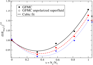
Figure 1: (color online) Ground-state energy per particle (in units of the free Fermi gas energy) scaled to the power of $3/5$ for normal spin-polarized neutron matter. Shown are QMC results at three different total densities $n_{1},n_{2},n_{3}$ (as points: black circles, red squares, blue diamonds, respectively), along with cubic fits to the Monte Carlo results (as lines: black solid, red dashed, blue dotted, respectively). Also shown using hollow symbols are the results for an unpolarized superfluid.

IV Phase competition

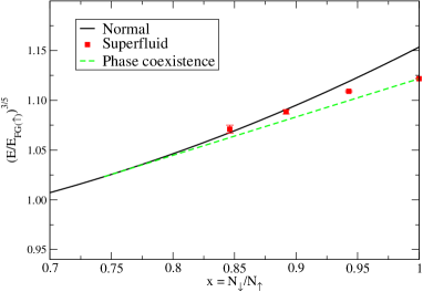
Figure 2: (color online) The construction of the mixed phase at density $n_{1}$. Shown is the energy of a normal neutron gas from Fig. 1 of the present work (black solid line), along with the homogeneous superfluid results of Refs. Gezerlis:2010 ; Gezerlis:2011 (red square points), and a tangent construction showing the phase coexistence curve (green dashed line). For large values of the relative fraction, the phase separated state is energetically favored with respect to a homogeneous polarized superfluid.

Having arrived at the functional dependence of the energy of a normal neutron gas on the relative fraction (thereby getting information on the $g(x,n)$ function defined in Eq. (1) and appearing in the rest of Sec. II), we can now use the simple cubic fits for the three densities $n_{1},n_{2},n_{3}$ to determine the competition between different phases. More specifically, Fig. 1 shows the behavior of the NP (normal polarized) equation of state. From the hollow points on the same figure we also have access to the energy of the SF (unpolarized superfluid) phase. Using these two dependences, we can find out the critical values of the relative fraction ($x_{c1},x_{c2},x_{c3}$, respectively) at the three densities we are studying. Above a critical relative fraction the system phase separates into a mixture of SF and NP, whereas below that value the neutron gas is normal, and therefore does not exhibit any of the widely studied features of a superfluid in the neutron star crust.

To determine $x_{c}$ we need the functional dependence of $g(x,n)$ on both $x$ and $n$, which is given by the interpolations for $n_{1}$, $n_{2}$ and $n_{3}$. Let us first focus on $n_{2}$. In Eq. (2) we also need the derivative with respect to $n$. We estimate this derivative by finite differences: $(g(x,n_{2})-g(x,n_{1}))/(n_{2}-n_{1})$ and $(g(x,n_{3})-g(x,n_{2}))/(n_{3}-n_{2})$. We estimate the derivatives for $SF$ used in Eq. 4 with a linear form in $1/(k_{F}a)$ and $k_{F}r_{e}$. In practice, $\frac{\partial g}{\partial n}$ is small and doesn’t affect the value of $x_{c}$ and $n_{SF}$ significantly. We can then solve the conditions for coexistence and find $x_{c}$ and $n_{SF}$. The numerical values show slight dependence on the interpolation method used. A simple cubic fit as a function of $x$ gives $x_{c2}=0.78$ and $n_{SF}=2.17\times 10^{-3}$ fm^-3. A three parameter fit in $(1,x,x^{5/3})$ motivated by Giorgini:2008 ; Lobo:2006 gives $x_{c2}=0.77$ and $n_{SF}=2.18\times 10^{-3}$ fm^-3. This gives some idea about the errors made in the interpolation: we estimate our error bar on $x_{c}$ to be $0.02$ for the three densities. This detailed procedure gives results very similar to a simpler procedure, namely constructing a tangent to the constant density $NP$ curve for $g(x,n)$ passing through the value of $g_{SF}(n)$ at the same density, which gives $x_{c2}=0.78$. The close agreement between the two approaches stems from the fact that $\frac{\partial g}{\partial n}$ is small — for $\frac{\partial g}{\partial n}=0$, the coexistence curve is given exactly by the tangent construction Bulgac:2007 . Therefore, we will use the tangent construction to find $x_{c}$ for $n_{1}$ and $n_{3}$ below.

This analysis requires that for $x<x_{c}$ the normal phase is thermodynamically stable. That is, the eigenvalues of the matrix $\frac{d^{2}{\cal{E}}}{dn_{i}dn_{j}}$ are positive. For $n=n_{2}$ we can check and have checked explicitly that this is the case. Finally, we find $\delta\mu$ at $x_{c2}$ is given by $\delta\mu_{c2}/E_{F}=0.16(2)$ where $E_{F}=({k_{F}^{2}}/{2m})$. Comparing with $\Delta_{SF2}/E_{F}\sim 0.23$ obtained from Ref. Gezerlis:2010 , we see that $\Delta_{SF2}>\delta\mu_{c2}$ satisfying the third condition for coexistence.

In Fig. 2 we have plotted as a black solid line the $n_{1}$ results from Fig. 1; at this density the perturbative $S=1,M_{S}=0$ correction in the Hamiltonian mentioned in Sec. III is the smallest, leading to the highest degree of confidence in the accuracy of our microscopic results. We focus on large values on the $x$-axis for reasons that will soon become clear. We also show as red square points the unpolarized superfluid result from Ref. Gezerlis:2010 (at $x=1$) and the homogeneous polarized superfluid results of Ref. Gezerlis:2011 (at smaller $x$). In addition, we show a coexistence curve which is arrived at by a tangent construction from the unpolarized superfluid to the normal polarized curve when the $y$-axis is chosen as we have Bulgac:2007 . This coexistence line meets the NP curve at $x_{c1}=0.74$ ($\delta\mu_{c1}/E_{F}=0.2$). As can be clearly seen in this Figure, the coexistence line lies below the homogeneous polarized superfluid Quantum Monte Carlo results, implying that these are not energetically favored (foreseeing this possibility, Ref. Gezerlis:2011 included a critical assumption explicitly excluding the possibility of phase separation). This situation follows the behavior of ultracold fermionic gases at unitarity: Lobo:2006 ; Pilati:2008 ; Giorgini:2008 there the critical value of the relative fraction was closer to $x_{c}=0.44$. The value we find is different for a variety of reasons: first, $n_{1}$ corresponds to $k_{F}a=-5$, which is somewhat smaller than $k_{F}a=\infty$. More importantly, the neutron-neutron interaction is characterized by a finite effective range and the presence of higher partial waves. The latter point explains why when we repeat this exercise for $n_{2}$ ($k_{F}a=-7.4$) and $n_{3}$ ($k_{F}a=-10$) the corresponding results (from tangent constructions) for the critical fraction are $x_{c2}=0.78$ ($\delta\mu_{c2}/E_{F}=0.16$) and $x_{c3}=0.88$ ($\delta\mu_{c3}/E_{F}=0.07$), respectively. The trend appears to be that at larger density (stronger coupling) the critical fraction is moving toward 1, implying that farther down toward the core of the neutron star polarized neutron matter quickly becomes normal for the vast majority of possible polarizations.

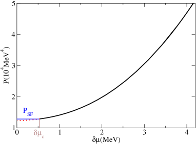
Figure 3: (color online) Pressure as a function of $\delta\mu$ for fixed $\mu=1.94$ MeV. For $\delta\mu>\delta\mu_{c}=0.53$ MeV the unpaired phase (bold black curve) has a higher pressure. At $\delta\mu_{c}$ [marked by the vertical line (brown online)], the $SF$ and the $NP$ phases can coexist. For smaller $\delta\mu$, the pressure of the $SF$ phase marked by the horizontal line (blue online) is larger than the pressure of the $NP$ phase marked by the dashed line (red online), and the $SF$ phase is favored. On the other extreme for $\delta\mu=4.18$ MeV, $x=0.0005$. We choose $\mu$ so that the density of the normal phase at $\delta\mu_{c}$ is $n_{2}$.

The value of $\delta\mu_{c}$ is relevant for neutron star phenomenology since whether $\delta\mu$ is greater or less than $\delta\mu_{c}$ determines the phase. This is seen more simply in the grand canonical ensemble where we can compare the pressure as a function of the chemical potentials. In Fig. 3 we plot the pressure as a function of $\delta\mu$ for fixed $\mu=1.94$ MeV. For this value of $\mu$ the density of the superfluid phase at the critical $\delta\mu$ is $n_{2}$. For $\delta\mu<\delta\mu_{c}$ the pressure of the $SF$ phase is larger and the system is unpolarised. Even if the magnetic field is not large enough to polarize the system, certain thermal observables, for example the specific heat, are sensitive to the difference between $\delta\mu$ and $\delta\mu_{c}$.

Determining the critical relative fractions is also relevant: if a magnetic field is strong enough to polarize neutron matter sufficiently ($x\leq x_{c}$), the gas ceases to be superfluid even at zero temperature. At such large magnetic fields, processes that rely on the presence of a bulk superfluid in the inner core of neutron stars, for example a recently proposed heat-conduction mechanism which requires superfluid phonons Aguilera:2009 , would no longer be operational. On a different note, a precise determination of these fractions (along with the rest of the equation of state) is also significant for Skyrme functional practitioners: for the region where the NP phase is the true ground state of the system, the results shown in Fig. 1 are a microscopic constraint to nuclear energy-density functional theory, which can help improve its predictions on neutron-rich heavy nuclei.

V Summary & Conclusions

In summary, we have studied spin-polarized low-density neutron matter at many values of the polarization. Our Quantum Monte Carlo approach provides tight upper bounds which are expected to be quite close to the true ground state-energy of the system. At very-low density the Hamiltonian becomes quite simple and we include its dominant well-known terms. We have calculated the energy as a function of polarization using the AV4^′ interaction at three different densities.

One of our main results is a determination of the critical relative fraction values above which the system phase separates into an unpolarized superfluid and a polarized normal neutron gas. Above these values, a homogeneous polarized superfluid is found not to be energetically favored. Below these values, the neutron gas is completely normal. Both these facts can lead to astronomically important consequences. Importantly, the trend of our results seems to imply that at slightly larger densities $x_{c}$ would be very close to one: this would mean that even at zero temperature a small polarization would be enough to close the superfluid pairing gap, and thus easily lead to larger polarization. In a non-astrophysical context, it is conceivable that our results could be tested directly by using ultracold fermionic atom gases with unequal spin populations and a finite effective range. In cold atoms, Quantum Monte Carlo simulations of spin-polarized matter have in recent times been repeatedly used as input to computationally less demanding density-functional theory approaches. Similarly, we expect that the results presented in this work can also be used as input to self-consistent mean-field models of nuclei.

A possible direction for future work, that would be interesting to both nuclear astrophysicists and Skyrme practitioners, would be a study of the behavior of polarized and unpolarized superfluid and normal neutron matter in an external periodic potential. Such a study of the static response of neutron matter could also in principle be guided (or guide) analogous research related to optical lattice experiments with cold atoms.

In the neutron star context, it will be useful to analyze the finite temperature phase diagram to understand how the specific heat is modified as a function of the chemical potential splitting, and how this modification affects transient phenomena in the neutron star crust.

- (1) S. Giorgini, L. P. Pitaevskii, and S. Stringari, Rev. Mod. Phys. 80, 1215 (2008).
- (2) S. Fantoni, A. Sarsa, and K. E. Schmidt, Phys. Rev. Lett. 87, 181101 (2001).
- (3) I. Vidaña, A. Polls, and A. Ramos, Phys. Rev. C 65, 035804 (2002).
- (4) A. Rios, A. Polls, and I.Vidaña, Phys. Rev. C 71, 055802 (2005).
- (5) M. G. Alford, J. Berges, K. Rajagopal, Nucl. Phys. B558, 219-242 (1999).
- (6) A. Gezerlis, Phys. Rev. C 83, 065801 (2011).
- (7) C. J. Pethick, N. Chamel, S. Reddy, Prog. Theor. Phys. Suppl. 186, 9-16 (2010).
- (8) V. Cirigliano, S. Reddy, and R. Sharma, Phys. Rev. C 84, 045809 (2011).
- (9) E. F. Brown and A. Cumming, Astrophys. J. 698, 1020 (2009).
- (10) D. N. Aguilera, V. Cirigliano, J. A. Pons, S. Reddy, and R. Sharma, Phys. Rev. Lett. 102, 091101 (2009).
- (11) M. G. Alford, S. Reddy, and K. Schwenzer, arXiv:1110.6213 (2011).
- (12) J. Carlson, J. Morales, Jr., V. R. Pandharipande, and D. G. Ravenhall, Phys. Rev. C 68, 025802 (2003).
- (13) A. Gezerlis and J. Carlson, Phys. Rev. C 77, 032801(R) (2008).
- (14) P. F. Bedaque, H. Caldas, and G. Rupak, Phys. Rev. Lett. 91, 247002 (2003).
- (15) R. Sharma and S. Reddy, Phys. Rev. A78, 063609 (2008).
- (16) A. Bulgac, M. M. Forbes, and A. Schwenk, Phys. Rev. Lett. 97, 020402 (2006).
- (17) A. Bulgac and M. M. Forbes, Phys. Rev. Lett. 101, 215301 (2008).
- (18) M. Bender, P.-H. Heenen, and P.-G. Reinhard, Rev. Mod. Phys. 75, 121 (2003).
- (19) B. Friedman and V. R. Pandharipande, Nucl. Phys. A361, 502 (1981).
- (20) A. Akmal, V. R. Pandharipande, and D. G. Ravenhall, Phys. Rev. C 58, 1804 (1998).
- (21) A. Schwenk and C. J. Pethick, Phys. Rev. Lett. 95, 160401 (2005).
- (22) J. Margueron, E. van Dalen and C. Fuchs, Phys. Rev. C 76, 034309 (2007).
- (23) M. Baldo and C. Maieron, Phys. Rev. C 77, 015801 (2008).
- (24) E. Epelbaum, H. Krebs, D. Lee, and U. -G. Meissner, Eur. Phys. J. A 40, 199 (2009).
- (25) E. Epelbaum, H.-W. Hammer, and U. -G. Meissner, Rev. Mod. Phys. 81, 1773 (2009).
- (26) T. Abe and R. Seki, Phys. Rev. C 79, 054002 (2009).
- (27) S. Gandolfi, A. Yu. Illarionov, F. Pederiva, K. E. Schmidt, and S. Fantoni, Phys. Rev. C 80, 045802 (2009).
- (28) A. Rios, A. Polls, and I. Vidaña, Phys. Rev. C 79, 025802 (2009).
- (29) K. Hebeler and A. Schwenk, Phys. Rev. C 82, 014314 (2010).
- (30) N. Chamel, S. Goriely, and J.M. Pearson, Nucl. Phys. A812, 72 (2008).
- (31) M. M. Forbes, A. Gezerlis, K. Hebeler, T. Lesinski, and A. Schwenk, under preparation (2011).
- (32) L. Luo and J. E. Thomas, J. Low Temp. Phys. 154, 1 (2009).
- (33) N. Navon, S. Nascimbène, F. Chevy, and C. Salomon, Science 328, 729 (2010).
- (34) J. Carlson and S. Reddy, Phys. Rev. Lett. 100, 150403 (2008).
- (35) A. Schirotzek, Y. I. Shin, C. H. Schunck, and W. Ketterle, Phys. Rev. Lett. 101, 140403 (2008).
- (36) Y. Shin, C. H. Schunck, A. Schirotzek, and W. Ketterle, Nature 451, 689 (2008).
- (37) J. Carlson, S. Y. Chang, V. R. Pandharipande, and K. E. Schmidt, Phys. Rev. Lett. 91, 050401 (2003).
- (38) G. E. Astrakharchik, J. Boronat, J. Casulleras, and S. Giorgini, Phys. Rev. Lett. 93, 200404 (2004).
- (39) J. Carlson and S. Reddy, Phys. Rev. Lett. 95, 060401 (2005).
- (40) C. Lobo, A. Recati, S. Giorgini, and S. Stringari, Phys. Rev. Lett. 97, 200403 (2006).
- (41) S. Pilati and S. Giorgini, Phys. Rev. Lett. 100, 030401 (2008).
- (42) A. Gezerlis, S. Gandolfi, K. E. Schmidt, and J. Carlson, Phys. Rev. Lett. 103, 060403 (2009).
- (43) B. Marcelis, B. Verhaar, and S. Kokkelmans, Phys. Rev. Lett. 100, 153201 (2008).
- (44) T. D. Cohen, Phys. Rev. Lett. 95, 120403 (2005).
- (45) A. Bulgac and M. M. Forbes, Phys. Rev. A 75, 031605 (2007).
- (46) R. B. Wiringa and S. C. Pieper, Phys. Rev. Lett. 89, 182501 (2002).
- (47) A. Gezerlis and J. Carlson, Phys. Rev. C 81, 025803 (2010).
- (48) M. M. Forbes, S. Gandolfi, and A. Gezerlis, Phys. Rev. Lett. 106, 235303 (2011).