TESIS

A mi hermano

Preface

This dissertation reports the research I have carried out as a PhD student in the Statistical Field Theory Group of the UCM, where I have been privileged to work and learn under the guidance of Luis Antonio Fernández and Víctor Martín. They not only form a truly remarkable scientific partnership, but have also been the best advisors I could ever have hoped to have.

My work during this time constitutes an attempt to make some headway in the field of complex condensed matter systems, concentrating on disordered spin models and taking a Monte Carlo approach. In particular, this dissertation deals with two archetypical systems: the diluted antiferromagnet in a field and the Edwards-Anderson spin glass. The former is studied with Tethered Monte Carlo, a formalism developed during this thesis.

As to the Edwards-Anderson spin glass, I have been fortunate to have access to Janus, a special-purpose machine that outperforms conventional computing architectures by several orders of magnitude in the Monte Carlo simulation of spin systems. This would be akin to being one of a few particle physicists with access to a newer, vastly more powerful collider (si parva licet componere magnis) and has allowed our group to tackle head-on a much studied model and still see some new physics. From the point of view of a PhD student, it has been a unique learning opportunity. Janus is the fruit of a collaboration of physicists and engineers from five universities in Spain and Italy. The project is directed by Alfonso Tarancón and has as scientific coordinators Víctor Martín Mayor, Giorgio Parisi and Juan Jesús Ruiz Lorenzo. My own participation has been, of course, only as a very junior member of a large collaboration, so I only include in this dissertation those physical studies where I carried out a major fraction of the work.

Agradecimientos

Esta tesis sólo ha sido posible gracias al constante e inestimable apoyo de muchas personas. En primer lugar, Luis Antonio Fernández y Víctor Martín merecen una nueva mención por su dedicación y accesibilidad, que ha ido mucho más allá de la habitual relación entre directores y doctorando. Mi grupo inmediato de trabajo lo completa Beatriz Seoane, brillante estudiante a quien espera una muy prometedora carrera científica.

Durante estos años he sido miembro del Departamento de Física Teórica I de la Universidad Complutense de Madrid, donde recibí una acogida ejemplar. Siento un agradecimiento especial hacia nuestro director, Antonio Muñoz, en cuyo despacho fui un intruso durante tres años, hasta que llegó el prometido traslado al módulo oeste de la facultad. No puedo dejar de recordar a Chon, una auténtica institución de la facultad que ha dejado huella en generaciones de físicos teóricos.

Agradezco también a todos los miembros de la Janus Collaboration todo lo que he aprendido de ellos. Dentro de ella, quiero hacer mención especial a los estudiantes que me han precedido, Antonio Gordillo y Sergio Pérez; así como a los que me siguen, Raquel Álvarez, José Miguel Gil y Jorge Monforte. también a Juan Jesús Ruiz, quien se tomó la molestia de preparar un cursillo intensivo sobre vidrios de espín para los miembros noveles. Estoy seguro de que no hablo solamente por mí cuando digo que en ese par de días nos aclaró muchas cosas con las que llevábamos peleando largo tiempo. Valoro, asimismo, enormemente haber tenido la oportunidad de aprender a través de la interacción con científicos de primer nivel como Enzo Marinari, Denis Navarro, Giorgio Parisi y Lele Tripiccione.

Por supuesto, Janus no habría sido posible sin la visión y carácter emprendedor de su director, Alfonso Tarancón, quien, no contento con ello, dirige también el Instituto de Biocomputación y Física de Sistemas Complejos (BIFI) en la Universidad de Zaragoza. A esta institución, de la que soy miembro, debo agradecer los enormes recursos computacionales que ha puesto a mi disposición durante esta tesis (que, aparte de Janus, se cuentan por varios millones de horas de CPU). Quiero recordar especialmente a los administradores de Piregrid: Jaime Ibar, Patricia Santos y Rubén Vallés.

Agradezco mucho a Leticia Cugliandolo y a Claudio Chamon, así como a todos los miembros de sus grupos, su hospitalidad y enseñanzas en sendas estancias en el LPTHE de la Université Pierre et Marie Curie (París) y en el Condensed Matter Theory Group de la Boston University.

También quiero agradecer a José María Martín y a Luis Garay, con quienes di mis primeros pasos hacia una carrera investigadora durante la licenciatura. Asimismo, agradezco a Antonio Dobado y a Felipe Llanes haberme introducido en el mundo de la docencia, con mi participación como ayudante en sus asignaturas de Electrodinámica Clásica y Mecánica Cuántica.

Mis amigos en Madrid y La Coruña han sido un pilar imprescindible durante todo este tiempo. Muchas gracias a todos, en especial a Antonio Arévalo, Eva Béjar, Pedro Feijoo, Rosa Gantes, Carlos Lezcano, Jesús Pérez y Antón Sanjurjo.

Dejo para el final al grupo más importante: mi familia. He sido afortunado en muchas cosas en mi vida, pero en nada tanto como en el cariño y apoyo de la familia que me ha tocado tener. Todos ellos tendrán siempre mi más sentido agradecimiento, en especial mis padres, que tantos sacrificios han hecho por mí. A mi hermano, y amigo, Daniel va dedicada esta tesis.

Durante este trabajo he estado financiado primero por una beca del BIFI y luego por una beca FPU del Ministerio de Educación. También he recibido apoyo de los proyectos fis2006-08533 y fis2009-12648 del MICINN y de los Grupos UCM – Banco de Santander. Agradezco finalmente a la Red Española de Supercomputación el haberme concedido alrededor de cuatro millones de horas de cálculo en el ordenador Mare Nostrum.

David Yllanes Mosquera
Universidad Complutense, Madrid, junio de 2011

Contents

toc

List of Figures

lof

List of Tables

lot

Notation

• Canonical expectation value of $O$ 34

• Canonical expectation value of $O$ for the applied field $h$ 56

• Tethered expectation value for smooth magnetisation $\hat{m}$ 58

• Numerical estimator for $\langle O\rangle$ 242

• Summation restricted to first neighbours 34

• Average over the quenched disorder 38

• Spin configuration 33

• Replicon exponent, equivalent to $\theta(0)$ 168

• Critical exponent of the specific heat 36

• Tethered field 59

• Binder ratio 65

• Critical exponent of the order parameter 36

• Inverse temperature, $\beta=1/T$ 33

• Averaging consecutive measurements of an observable in
  blocks of either constant or geometrically growing length 242

• Specific heat 64

• Two-time spatial correlation 169

• Spatial autocorrelation of the overlap field (equilibrium) 194

• Spatial autocorrelation of the overlap field (dynamics) 168

• Magnetic susceptibility 64

• Diagonal chi-square fit-goodness estimator 258

• Complete chi-square fit-goodness estimator 257

• Spin-glass susceptibility 167

• Link correlation function 215

• Two-time correlation function 167

• Spatial dimension of the system 33

• Degrees of freedom in a fit 257

• Critical exponent of the equation of state at $T=T_{\text{c}}$ 36

• Total energy of the system 33

• Conditional expectation value of $O$ at fixed $q$ 195

• Quenched occupation variables 105

• Anomalous dimension 36

• Gibbs free-energy density 34

• Finite-size scaling 37

• Critical exponent of the system’s response 36

• Applied field 34

• Staggered component of the applied field 105

• Coupling between sites ${\boldsymbol{x}}$ and ${\boldsymbol{y}}$ 34

• Smallest non-zero momentum 65

• Linear size of the square lattice 33

• Magnetisation 34

• Monte Carlo sweep, i.e., update of the whole lattice 48

• A single evaluation of an observable during the simulation 33

• Smooth magnetisation 57

• Staggered magnetisation 105

• Number of degrees of freedom (i.e., lattice nodes) 33

• Critical exponent of the correlation length 35

• A function of the spin configuration, $O(\{s_{\boldsymbol{x}}\})$ 33

• Tethered weight 47

• Helmholtz free energy or efective potential 35

• Value of observable $O$ along the simulation $O(t)=O(\{s_{\boldsymbol{x}}(t)\})$ 43

• Probability density function of $\hat{m}$ 57

• Smoothed probability density function of the spin overlap 195

• Probability that a link is occupied (cluster methods) 86

• Probability that a node is occupied (DAFF) 105

• Probability density function 57

• Parity of site ${\boldsymbol{x}}$ 105

• Spin overlap 153

• Link overlap 159

• Overlap field 167

• Bath of Gaussian demons 57

• Copies of the system that evolve with the same set of $J_{{\boldsymbol{x}}{\boldsymbol{y}}}$ 167

• Ising spin, $s_{\boldsymbol{x}}=\pm 1$ 33

• A particular configuration of the disorder variables 38

• Temperature 33

• Measurement time 160

• Critical temperature 35

• Heaviside step function 47

• Hyperscaling violations exponent 107

• Algebraic decay of the fixed-$q$ connected correlations 198

• Tethered Monte Carlo 46

• Waiting time 160

• Interaction energy of the spins 34

• Variance of $O$, conditioned to fixed $q$ 222

• Correlation length 35

• Second-moment correlation length 65

• Coherence length (dynamical) 168

• Stiffness exponent of the droplet picture 158

• Partition function 33

• Two-time correlation length 170

Part I Introduction

CHAPTER I   General introduction

Modern physics is steadily broadening its scope and tackling increasingly complex systems, whose rich collective behaviour is not easily explained from the often simple nature of their constituent parts. Thus, a lot of attention is being focused on understanding, from a fundamental point of view, an extremely diverse class of problems, ranging from vortex glasses in high-temperature superconductors to biological macromolecules. The featured physical phenomena can be as exotic as the colossal magnetoresistance of some manganites [dagotto:01, coey:09, levy:02], or as familiar as the formation of glass [angell:95, debenedetti:97, debenedetti:01]. The latter constitutes a particularly conspicuous example of an everyday material whose microscopic description remains, in the words of P. W. Anderson [anderson:95], ‘probably the deepest and most interesting unsolved problem in solid state theory’. On a different vein, the study complex physical systems has deep relations to the field of computational complexity and NP-incompleteness [mezard:02, zecchina:06].

The enormous variety of problems, often straddling the boundaries between physics, chemistry and biology, seems to suggest that the label of ‘complex system’ bears little meaning, since it seems that each class of systems must surely be studied separately. Actually, behind the diversity we can find key unifying features, which has motivated attempts to find some solid common ground for a joint treatment of complexity.

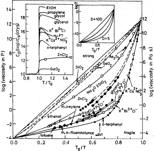
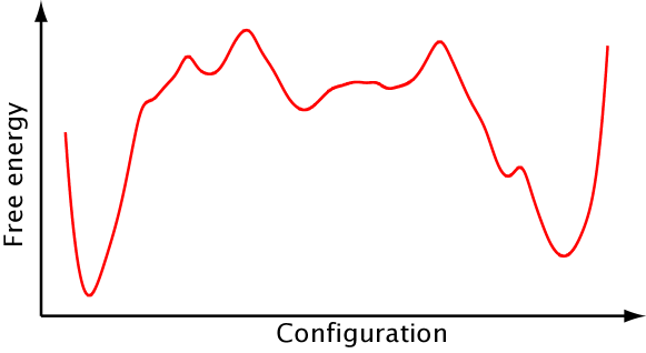
Figure 1.1: Angell plot, taken from [angell:95], showing the viscosity of many glass-forming liquids. The horizontal axis is rescaled in terms of a glass temperature $T_{\text{g}}$, defined as that where the system’s viscosity reaches the value of $10^{13}$ P. In this representation, the deviation from the ideal Arrhenius law (leftmost straight line) seems completely encoded by the derivative at $T_{\text{g}}$. Notice that the values of the viscosity span $15$ orders of magnitude.

Figure 1.2: Idealised picture of a complex system. The free-energy profile contains many local minima, which define metastable states with exponentially long escape times.

In this sense, the best hope of the fundamental physicist is the notion of universality [cardy:96, amit:05, zinn-justin:05]. In general, a strict microscopic description of a complex system is a daunting task: one has to account for many degrees of freedom, whose interactions follow complicated laws. Fortunately, one can often identify a few crucial scaling variables, whose evolution encodes the behaviour of the whole system. More than that, by expressing all the more complicated quantities in terms of these, very different systems can be shown to have the same qualitative behaviour. Hence, all these systems can be understood through the study of their simplest representative.

Perhaps the most striking example of this universal behaviour is the celebrated Angell plot, of which we show an example in Figure 1.2. In it, glass-forming liquids with completely different compositions and qualitatively different temperature dependencies of the viscous flow are classified according to their ‘fragility’. This is defined as the (logarithmic) derivative of the viscosity at the glass transition temperature and, as it turns out, it characterises the material’s deviation from the Arrhenius law, along 15 orders of magnitude. Scant few physical quantities have ever been measured along so wide a range but, beyond that, the figure encloses very deep physics.

For instance, fluctuation-dissipation relations [kubo:57] allow us to translate viscosity into time. Therefore, the plot is showing us a situation where relaxation times cross over from a microscopic to a macroscopic range. Notice that the scaling temperature in this plot is chosen as the point where the viscosity reaches $10^{13}$ P (equivalent to relaxation times of one hour). More than that, and one has to accept working out of equilibrium, which, in some fields, is a tough pill to swallow.

In the context of magnetic systems —where, unlike with glasses, one is sure of being below a phase transition— the off-equilibrium regime is a completely natural experimental environment and has been for some time. A classic application is the study of coarsening, a kind of dynamics characterised by the growth of compact coherent domains. In this case, an especially powerful version of universality operates, aptly called superuniversality [fisher:86]. According to it, all the spatial and temporal scales during the dynamics are encoded in the growth of a coherence length, which indicates the size of the coherent domains (cf. Chapter 9).

In general, we can say that the most common feature of complex systems is an incredibly slow dynamical evolution, or aging [struick:78, bouchaud:98]. The study of non-equilibrium relaxation is, thus, very important and often the only accessible experimental regime.

In order to explain this sluggishness, the most often invoked defining characteristic of complex systems is the picture of a ‘rugged free-energy landscape’ [frauenfelder:97, janke:08]. The configuration space is pictured as having many valleys, defining metastable states where a configuration is much more favourable than neighbouring ones (Figure 1.2). The system in its evolution, then, must jump from one local minimum to another through rare-event states, causing the slow dynamics.

The causes of this ruggedness are diverse. For some materials, it may be due to the presence of impurities or other defects, which hinder the physical evolution. In others, the sluggish behaviour has been modelled as a hierarchically constrained dynamics, consisting in the sequential relaxation of different degrees of freedom, from the fastest to the slowest [palmer:84].

Sometimes one of the valleys dominates and the free-energy profile is funnel shaped. This is the case, for instance, of protein folding, where the native configuration defines an absolute minimum. For other systems, on the other hand, there can be many equally favourable configurations, so one must take several metastable states into account even when defining the equilibrium. The difference between both cases is not idle: proteins quite obviously are able to fold into their equilibrium configuration very quickly (in human terms), while glassy systems with metastable behaviour are perennially out of equilibrium.

Since in this latter case the equilibrium phase is experimentally unreachable, determining what (if any) bearing it has on the dynamical evolution (what we shall call the ‘statics-dynamics relation’) is a non-trivial problem.

This discussion notwithstanding, we must caution the reader that Figure 1.2 is, at best, a metaphor. In order to turn it into real physics one must first, at the very least, identify one (or more) appropriate reaction coordinates capable of actually labelling the different minima. This requires a great deal of insight into the system’s physics and still leaves unresolved the non-trivial step of actually computing the free energy.

The quantitative investigation of these two issues (statics-dynamics and the free-energy landscape) will constitute the main themes of this dissertation. We shall work in the context of disordered magnetic systems, long considered prime examples of complexity. One may think that the introduction of disorder cannot be responsible for very exciting changes in a physical system. This is true in some cases (after all, even the most perfect experimental sample has some impurities, yet we can still talk of crystals or ferromagnets), but not in general. For some strongly disordered systems, we shall see, the impurities have a dramatic effect both in a technical sense (being a relevant perturbation in a renormalisation-group setting) and in a very physical sense. Consider, for instance, the example of Anderson localisation [anderson:58], capable of turning metallic systems into insulators.

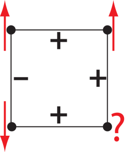
Figure 1.3: A small portion of a spin-glass lattice. The spins on the nodes can only take the ‘up’ or ‘down’ orientation. They are joined along nearest-neighbour links by a mixture of ferromagnetic ($+$) and antiferromagnetic ($-$) couplings. The former favour aligned pairs of spins and the latter favour antiparallel ones. With the arrangement shown in the figure there is no way of orienting the spins so that all of the bonds are satisfied.

One of the simplest mechanisms responsible for the complexity of disordered systems is that of frustration [toulousse:77], as very clearly illustrated in the case of spin glasses (see, e.g., [binder:86, mezard:87] and cf. Chapter 9). These are magnetic alloys in which the interactions between the spins are in conflict. The disorder manifests as a mixture of ferromagnetic and antiferromagnetic couplings. Thus, even for the lowest-energy configuration some of the bonds are necessarily frustrated, as we see in Figure 1.3. This makes it exceedingly difficult for the physical system to find the equilibrium state (and no less for the physicist performing a computation). Furthermore, many configurations have a similar degree of frustration and are therefore equally favourable, giving rise to a free-energy landscape with many relevant metastable states.

Yet not only the equilibrium is complicated but also the dynamical behaviour. In the case of spin glasses, to the aging behaviour we have to add phenomena such as rejuvenation or memory effects [jonason:98].

The choice of disordered magnetic systems as paradigmatic models for complexity is mainly due to their permitting more precise experimental studies than other classes of complex systems [mydosh:93, belanger:98]. There are both technical and physical reasons for this, as we shall see later.

On the theoretical front, on the other hand, these systems are at least easy to model with deceptively simple lattice systems. The solution of these models is another matter entirely. Indeed, disordered systems have often defied traditional, and powerful, analytical tools such a perturbation theory [dedominicis:06]. In the case of spin glasses, even the solution of such a gross simplification as the mean-field approximation has been a veritable tour de force [parisi:79b, parisi:80]. Other systems, such as the random field Ising model, are seemingly more amenable to a perturbative treatment [dedominicis:06, nattermann:97] but remain very poorly understood, the analytical approach failing to analyse the critical behaviour convincingly.

In the last decades, a third avenue has opened for basic research: the computational approach, of which the most salient example is Monte Carlo simulation [landau:05, rubinstein:07]. Unfortunately, in the case of disordered systems traditional Monte Carlo methods suffer from the same problems as experiments do, to an even greater degree. A simulation of a rugged free-energy landscape for a finite lattice will get trapped in the local minima, just as an experiment, with an escape time that grows as the exponential of the free-energy barrier, which in turn goes as a power of the lattice size. As a consequence, for many models of interest only very small systems can be thermalised, making extrapolation to the thermodynamical limit very complicated. Many simulation algorithms have been proposed to address this problem. However, as a general rule efficient innovations require some previous knowledge, or at least a somewhat detailed working hypothesis, of the underlying physics. Therefore, the investigation of new Monte Carlo dynamics must not be considered in isolation, but as an enterprise that should be undertaken jointly with a thorough study of challenging physical problems.

An alternative is simply to eschew equilibrium and attempt a Monte Carlo reproduction of an experimental dynamics. This is simple enough in principle, the most straightforward Monte Carlo dynamics being good mock-ups of the physical evolution, and has the advantage of considering the system in more controlled conditions that are possible in a laboratory. Unfortunately, current computers are several orders of magnitude too slow to reach the experimentally relevant time scales.

In short, the study of complex systems faces significant obstacles, both experimental and theoretical. From a fundamental point of view, far from discouraging further effort, these problems are at heart the reasons why these systems are so interesting, constituting a constant reminder that the traditional tools of statistical mechanics must be continuously complemented and expanded. This in addition to the fact that by ‘complex systems’ we encompass such everyday materials as glasses, as well as systems with great technological or medical relevance (colossal magnetoresistance oxides, proteins, etc.).

1.1  Scope of this thesis

This thesis is an attempt to provide a new outlook on complex systems, as well as some physical answers for certain models, taking a computational approach. We have focused on disordered systems, addressing two traditional ‘hard’ paradigmatic models in three spatial dimensions: the Edwards-Anderson spin glass and the diluted antiferromagnet in a field (the physical realisation of the random-field Ising model). These systems have been studied by means of large-scale Monte Carlo simulations, exploiting a variety of platforms (computing clusters, supercomputing facilities, grid computing resources and even a custom-built special-purpose supercomputer). In accordance to the above discussion, the physical study has been taken hand in hand with the development of new Monte Carlo methods.

Indeed, at the foundation of the work reported herein is the development of Tethered Monte Carlo, a general strategy for the study of rugged free-energy landscapes. This formalism provides a general method to guide the exploration of configuration space by constraining (tethering) one or more parameters. In particular, one selects a reaction coordinate (typically, but not necessarily, order parameters) capable of labelling the different local free-energy minima. A statistical ensemble is then constructed, permitting efficient Monte Carlo simulation where these coordinates are fixed, avoiding the need to tunnel between competing metastable states. From these tethered simulations the Helmholtz potential associated to the reaction coordinates is reconstructed, yielding all the information about the system.

This philosophy is applied first to ferromagnetic models (hardly complex systems, but extraordinary benchmarks nonetheless) and then to the diluted antiferromagnet in a field. There it is showed that the tethered approach, far from being a mere optimised Monte Carlo algorithm, is capable of providing valuable information that would be hidden from a traditional study, thus permitting a more complete picture of the physics. One of the more conspicuous examples of this is that pictures such as Figure 1.2, long treated as mere conceptual aides, have been turned into real computations of free-energy profiles.

The next part of this dissertation is concerned with the Edwards-Anderson spin glass. For this system, our physical understanding is not yet at a level that would permit a full tethered treatment. This notwithstanding, many pointers are taken from the tethered philosophy, particularly in regards to the analysis of physical results. For the Monte Carlo simulation, the strategy has been mainly one of sheer brute force. Our work on spin glasses has been conducted within the Janus Collaboration, a joint effort of researchers from five universities in Spain and Italy. This project has as its main goal the construction and exploitation of Janus, a special-purpose computer optimised for spin-glass simulations, where it outperforms conventional computers by several orders of magnitude.

Aside from having been carried out with slightly different methods, our work on spin glasses is complementary to the rest of this thesis in a major physical way: it makes a strong emphasis on off-equilibrium dynamics. Indeed, as we advanced in the previous discussion, experiments on spin glasses (and many other complex systems) are always performed in an off-equilibrium regime. Then, a very valid question arises: how relevant is it to know the unreachable equilibrium phase? Our outlook, as we said before, has been that equilibrium structures, though inaccessible, do condition the off-equilibrium evolution. This idea, long accepted as a working hypothesis, is turned into a quantitative statement with the finite-time scaling paradigm. Time is treated as a state variable, much as pressure or temperature in a traditional thermodynamical setting. A time-length dictionary links off-equilibrium results in the thermodynamical limit for finite times with equilibrium results for finite lattices.

The next section summarises the organisation of the rest of this dissertation. It should be noted that each section contains a more detailed topical introduction, expanding on the issues touched in this General Introduction.

1.2  Organisation of this dissertation

As discussed above, the work reported herein is concerned both with the study of paradigmatic complex systems in statistical mechanics (the DAFF and the spin glass) and with the development of new Monte Carlo and analysis methods. The rest of this dissertation is, therefore, organised thematically in the following way:

• Part I, including this General Introduction, has the purpose of motivating our study and presenting our outlook on complex systems and how they should be treated. We start by, very briefly, recalling some statistical mechanical concepts relevant to the study of complex systems (Chapter 2). This is followed by Chapter 3, already concerned with our Monte Carlo approach. In it we expand on the practical problems posed by the numerical simulation of rugged free-energy landscapes and motivate the tethered formalism as a way of removing or alleviating them. This last chapter contains some material from our paper [martin-mayor:11].

• Part II deals with our work on new Monte Carlo methods, motivated by the above considerations. We start by detailing the construction of the tethered formalism in Chapter 4. We then present a first demonstration of the method in a straightforward application: the $D=2$ Ising model (Chapter 5). This is, of course, a well understood system, so our aim is not so much presenting new physics as demonstrating our methods and how a tethered study can provide a complementary picture to canonical methods. Finally, Chapter 6 proves that the tethered formalism is compatible with advanced Monte Carlo algorithms, in this case cluster methods. We first introduced the Tethered Monte Carlo method in [fernandez:09] and we later presented it in a more general context in [martin-mayor:11]. Chapters 5 and 6 contain material from [fernandez:09] and [martin-mayor:09], respectively.

• Part III discusses the first class of complex systems we shall study: the diluted antiferromagnet in a field. In Chapter 7 we present the situation that existed prior to our work and demonstrate how this system is particularly ill-suited to a study with canonical methods. We then tackle the problem with the tethered formalism in Chapter 8, applying all the techniques introduced in Part II. This chapter is a much expanded version of [fernandez:11b], including some material from [martin-mayor:11], as well as some unpublished results.

• Part IV deals with spin glasses. In Chapter 9 we introduce these systems, stressing their peculiarities from an experimental point of view (with phenomena such as aging, rejuvenation, memory, etc.) and their resulting theoretical importance as paradigmatic complex systems. Chapter 10 deals in depth with one of the main themes of this thesis: the relationship between equilibrium and non-equilibrium and introduces the finite-time scaling framework. Finally, Chapter 11 studies in detail the structure of the spin-glass phase in three spatial dimensions. Our work on spin glasses, carried out within the Janus collaboration, was published in [janus:08b, janus:09b, janus:10, janus:10b]. Chapters 10 and 11 are a heavily reworked and reorganised version of the results in those papers, including some unpublished material.

• Finally, Chapter 12 contains our conclusions.

• We include several appendices. Appendix A gives some notes on how to assess thermalisation in Monte Carlo simulations. It starts reporting some standard definitions but then describes some new techniques for complex systems (first introduced in [janus:10]). Appendix B presents some techniques for analysing the strongly correlated data produced in the Monte Carlo simulation of disordered systems. The explained methods are illustrated with especially tough examples and case studies taken from our work. Appendix C contains some practical notes for an efficient numerical implementation of Tethered Monte Carlo. Finally, Appendix D introduces the Janus special-purpose computer used in our spin-glass simulations and Appendix E gathers all the technical information on these runs (parameters, thermalisation, etc.).

CHAPTER II   Statistical mechanics of disordered systems: basic definitions

In this chapter we briefly recall some general definitions that will we employed throughout this dissertation, with the main purpose of fixing the notation and introducing some notions particular to the study of disordered systems. For general references on statistical mechanics or the theory of critical phenomena see, e.g., [landau:80, huang:87, amit:05, lebellac:91, zinn-justin:05, cardy:96]. For disordered systems, see [mezard:87, young:98, dedominicis:06, dotsenko:01].

2.1  Statistical mechanics and critical phenomena

We consider a system whose configuration can be specified by $N$ degrees of freedom $\{s_{\boldsymbol{x}}\}$. In the canonical ensemble, the behaviour of the system is encoded in the partition function

$$Z=\sum_{\{s_{\boldsymbol{x}}\}}\mathrm{e}^{-\beta E(\{s_{\boldsymbol{x}}\})}.$$ (2.1)

In this equation, the sum is extended to all possible configurations, their relative weights depending on their energy $E$. The parameter $\beta=1/k_{\text{B}}T$ is the inverse temperature. We use units where the Boltzmann constant is $k_{\text{B}}=1$, so $\beta=1/T$.

Throughout this dissertation we study Ising spins, $s_{\boldsymbol{x}}=\pm 1$, on a square lattice of $N=L^{D}$ nodes, where $D$ is the spatial dimension. Therefore, in the following we often use the language and notation of magnetic systems, even if much of what we say can be applied to more general systems.

We define an observable $O(\{s_{\boldsymbol{x}}\})$ as any function of the spin configuration. In the context of Monte Carlo simulations, where we estimate $Z$ by means of a random walk in configuration space, we use the word measurement for a single evaluation of the observable during the simulation.

The total energy of the system can often be written in the following way

$$E(\{s_{\boldsymbol{x}}\})=U(\{s_{\boldsymbol{x}}\})-hX(\{s_{\boldsymbol{x}}\}),$$ (2.2)

where $U$ is the interaction energy of the spins and $h$ is an external field, coupled to some reaction coordinate $X$. In our case, $U$ will be of the form of a two-spin interaction

$$U(\{s_{\boldsymbol{x}}\})=-\sum_{{\boldsymbol{x}},{\boldsymbol{y}}}J_{{\boldsymbol{x}}{\boldsymbol{y}}}s_{\boldsymbol{x}}s_{\boldsymbol{y}},$$ (2.3)

where the $J_{{\boldsymbol{x}}{\boldsymbol{y}}}$ are the couplings. For instance, for the ferromagnetic Ising model, $J_{{\boldsymbol{x}}{\boldsymbol{y}}}=1$ if ${\boldsymbol{x}}$ and ${\boldsymbol{y}}$ are nearest neighbours on the lattice and zero otherwise. We represent this sort of nearest-neighbours interaction as

$$U(\{s_{\boldsymbol{x}}\})=-\sum_{\braket{{\boldsymbol{x}},{\boldsymbol{y}}}}s_{\boldsymbol{x}}s_{\boldsymbol{y}}.$$ (2.4)

In this context, the most straightforward reaction coordinate is the magnetisation $M$,

$$M(\{s_{\boldsymbol{x}}\})=\sum_{\boldsymbol{x}}s_{\boldsymbol{x}},$$ (2.5)

although we shall consider other kinds.

Therefore, the canonical ensemble describes the system at fixed temperature and applied field. The basic thermodynamic quantity is the free-energy density

$$F_{N}(\beta,h)=\frac{1}{N}\log Z(\beta,h).$$ (2.6)

The average value of an observable in the canonical ensemble is denoted by

$$\braket{O}=\frac{1}{Z}\sum_{\{s_{\boldsymbol{x}}\}}O(\{s_{\boldsymbol{x}}\})\ \mathrm{e}^{-\beta E(\{s_{\boldsymbol{x}}\})}.$$ (2.7)

For quantities such as $M$ or $E$ we distinguish the extensive version from the density by the use of uppercase and lowercase symbols, respectively,

$$M =Nm, E =Ne.$$ (2.8)

Notice that we do not use this convention for the free energy, $F_{N}$, which is also a density, but only for observables.

2.1.1 Legendre transformation

Throughout Part II, we shall find it interesting to consider an alternative ensemble where it is the reaction coordinate $m$, and not the field $h$, which is kept fixed. In classical thermodynamics, this is accomplished through the Legendre transformation, defining a new basic potential.

$$\varOmega_{N}(\beta,m)=\beta mh-F_{N}(\beta,h).$$ (2.9)

We say $\varOmega_{N}$ is the Helmholtz free energy ($F_{N}$ is the Gibbs free energy). Since these names are often exchanged in the literature, we avoid confusion by reserving the name ‘free energy’ for $F_{N}$, while we shall call $\varOmega_{N}$ ‘effective potential’, borrowing the name from the context of quantum field theory. If $F_{N}$ is a convex function of $h$, this operation allows us to define $\varOmega_{N}$ as a convex function of $m$. However, for disordered systems with rugged free-energy landscapes $\varOmega_{N}$ is never convex for finite $N$. Therefore, we shall consider the following alternative representation of the transformation,

$$Z_{N}(\beta,h)=\mathrm{e}^{NF_{N}(\beta,h)}=\int\mathrm{d}m\ \mathrm{e}^{N[\beta hm-\varOmega_{N}(\beta,m)]}\,,$$ (2.10)

The conjugate nature of $m$ and $h$ can be summarised by the following formulae

$$\braket{m} =\left.\frac{1}{\beta}\frac{\partial F_{N}}{\partial h}\right|_{\beta}, \braket{h}_{m} =\left.\frac{1}{\beta}\frac{\partial\varOmega_{N}}{\partial m}\right|_{\beta},$$ (2.11)

where by $\braket{\cdots}_{m}$ we denote the expectation value in the fixed-$m$ ensemble defined by $\varOmega_{N}$.

2.1.2 Critical phenomena and exponents

We shall often consider the behaviour of physical systems in the neighbourhood of a second-order phase transition, where the system approaches continuously a state at which the scale of correlations becomes unbounded. In particular, if we write the correlation between sites ${\boldsymbol{x}}$ and ${\boldsymbol{y}}$ as

$$\braket{s_{\boldsymbol{x}}s_{\boldsymbol{y}}}\xrightarrow{\ \ |{\boldsymbol{x}}-{\boldsymbol{y}}|\to\infty\ \ }\exp(-|{\boldsymbol{x}}-{\boldsymbol{y}}|/\xi),$$ (2.12)

then, in the thermodynamic limit, the correlation length $\xi$ diverges as we approach the critical temperature $T_{\text{c}}$. We characterise the divergence by a critical exponent $\nu$

$$\xi\sim|T-T_{\text{c}}|^{-\nu}\,.$$ (2.13)

This behaviour is not exclusive of the correlation length, many other quantities either diverge or vanish as we approach $T_{\text{c}}$. Therefore, one defines additional critical exponents:

• Response of the system to an infinitesimal field $h$ (for instance, the magnetic susceptibility),

  $$\chi\sim|T-T_{\text{c}}|^{-\gamma}.$$ (2.14)

• Specific heat

  $$C\sim|T-T_{\text{c}}|^{-\alpha}.$$ (2.15)

• Order parameter (for instance, the magnetisation)

  $$m\sim(T_{\text{c}}-T)^{\beta}.$$ (2.16)

  Unfortunately, this exponent uses the same symbol as the inverse temperature in what is a completely universal usage, but the context should always make clear which is the referred quantity.

• Precisely at $T=T_{\text{c}}$, the decay of the correlation function is characterised by the anomalous dimension

  $$\braket{s_{\boldsymbol{x}}s_{\boldsymbol{y}}}\sim|{\boldsymbol{x}}-{\boldsymbol{y}}|^{-(D-2+\eta)}.$$ (2.17)

• Finally, again at $T=T_{\text{c}}$, the order parameter has a critical dependence on the applied field $h$

  $$m\sim h^{1/\delta}.$$ (2.18)

We have thus defined six different critical exponents. However, very general considerations let us establish the so-called scaling relations

$$2\beta+\gamma =2-\alpha,$$ (2.19a)

$$2\beta\delta-\gamma =2-\alpha,$$ (2.19b)

$$\gamma =\nu(2-\eta),$$ (2.19c)

$$\nu D =2-\alpha.$$ (2.19d)

The last of these, involving the dimension $D$, is called a hyperscaling relation. Using (2.19), we see that for a general system, only two critical exponents are independent.

In mean-field theory the exponents are $\beta=\nu=1/2$, $\gamma=1$, $\alpha=\eta=0$, $\delta=3$. Above some (model-dependent) upper critical dimension $D_{\text{u}}$ all systems are described by these mean-field exponents. Notice that they do not depend on $D$, in contrast with the hyperscaling law. Usually, $D_{\text{u}}=4$, but we shall see that this is not the case for disordered systems. Finally, below the lower critical dimension $D_{\text{l}}$ there is no transition.

2.1.3 Finite-size scaling

One of the most useful tools for the study of critical phenomena is the scaling hypothesis. According to this, in the thermodynamic limit the correlation length $\xi_{\infty}$ is the only characteristic length of the system in the neighbourhood of $T_{\text{c}}$ (in this regime, the correlation length is large in units of the lattice spacing and the system ‘forgets’ about the lattice).

In a finite lattice, the corresponding finite-size scaling (FSS) ansatz states that the finite-size behaviour is determined by the ratio $L/\xi_{\infty}$. If the ratio is large, the finite-size effects are not important and the finite system is not essentially different from the thermodynamic limit. If the ratio is small, however, we say we are in the FSS regime. There, an observable $O$ will behave as

$$\braket{O}^{(L)}\simeq L^{x_{O}/\nu}f_{O}(L/\xi_{\infty}),$$ (2.20)

where $x_{O}$ characterises the critical behaviour of $O$,

$$\braket{O}^{(\infty)}\sim|T-T_{\text{c}}|^{-x_{O}}.$$ (2.21)

Alternatively, using the definition of the critical exponent $\nu$ we can write

$$\braket{O}^{(L)}\simeq L^{x_{O}/\nu}\tilde{f}_{O}(L^{1/\nu}t),\qquad t=(T_{\text{c}}-T)/T_{\text{c}}.$$ (2.22)

The FSS ansatz can be derived using renormalisation-group techniques (see, for instance, [amit:05]).

Note that in a finite lattice one cannot really talk of a phase transition. There are no actual divergences of the physical quantities, only ever narrowing peaks whose position tends to the real critical point and whose height grows as $L^{x_{O}/\nu}$. In this sense, Eq. (2.22) encodes the behaviour in a crossover region of width $\sim~{}L^{-1/\nu}$ between the two phases. In the thermodynamical limit, this interval degenerates in a point and the crossover turns into a proper phase transition.

Finally, let us note that at the critical point $\xi_{\infty}\to\infty$, so the scaling hypothesis leads to the conclusion that the system exhibits scale invariance, since there is no characteristic length. This is an important observation for detecting the presence of a second-order transition.

2.2  Quenched disorder

Let us now consider a system with disorder. In addition to the spins $s_{\boldsymbol{x}}$, we need to specify additional variables $\mu_{i}$ that characterise the randomness. In our model Hamiltonian (2.2), these can be random couplings $J_{{\boldsymbol{x}}{\boldsymbol{y}}}$, vacancies in the lattice or even a random, site-dependent field $h_{\boldsymbol{x}}$.

In principle, for each configuration of the disorder variables (disorder realisation or sample) we will have a different partition function

$$Z_{\mu}=\sum_{\{s_{\boldsymbol{x}}\}}\mathrm{e}^{-\beta\mathcal{H}_{\mu}(\{s_{\boldsymbol{x}}\})}.$$ (2.23)

If the disorder variables exhibit a dynamical evolution in time scales short compared to the observation time (diffusion of impurities at high temperatures, for instance) we say the disorder is annealed. In this situation, we can treat the $\mu_{i}$ as additional dynamical variables and average over them, to obtain the complete partition function. We denote this disorder average by an overline, $\overline{(\cdots)}$, so the free energy of the system is

$$F_{N}=\frac{1}{N}\log\overline{Z_{\mu}}\,.$$ (2.24)

We are interested in the opposite limit, where the impurities show no dynamical evolution in experimental time scales. We say the disorder is quenched, so the free energy is different for each sample

$$F_{N}(\mu)=\frac{1}{N}\log Z_{\mu}\,.$$ (2.25)

This does not seem like a useful concept, because it seems to imply we would need a different model for each particular piece of material. What actually happens is that, for large enough systems, the physical properties do not depend on the $\mu_{i}$ anymore,

$$\lim_{N\to\infty}F_{N}(\mu)=F_{\infty}.$$ (2.26)

There is a simple argument for this in finite dimension, due to Brout [brout:59]. We divide the lattice in many macroscopic systems of size $1\ll R^{D}\ll N$. Then the free-energy density of the whole system will be the average of those of the $N/R^{D}$ subsystems, plus a contribution coming from interactions between them. If we assume that the interactions are short-range, this latter contribution is an interface energy, negligible in the large-$N$ limit. Therefore, computing the free-energy density of a very large lattice is essentially the same as averaging that of many smaller systems and the central limit theorem guarantees that

$$\overline{F^{2}_{N}(\mu)}-\overline{F_{N}(\mu)}^{2}\sim\frac{1}{N}\,.$$ (2.27)

We say the free energy self-averages.

So, the concept of quenched disorder is physically sound, but it implies a serious difficulty. In order to obtain physically meaningful results, we have to average the free energy, which is the same as averaging the logarithm of $Z_{\mu}$

$$F_{N}=\overline{F_{N}(\mu)}=\frac{1}{N}\overline{\log Z_{\mu}}\,.$$ (2.28)

The task of computing the average of a logarithm, unusual in statistical mechanics, is exceedingly difficult. There is, however, a way around it: the so-called replica method [kac:68, edwards:72]. This is based on the elementary relationship

$$\log Z=\lim_{n\to 0}\frac{Z^{n}-1}{n}.$$ (2.29)

For positive integer $n$, $Z^{n}_{\mu}$ can be expressed in terms of identical replicas of the system (sharing the same configuration of the $\mu_{i}$)

$$Z^{n}_{\mu}=\prod_{a=1}^{n}Z_{\mu}^{(a)}=\sum_{\{s_{\boldsymbol{x}}^{a}\}}\exp\biggl{[}-\beta\sum_{a=1}^{n}\mathcal{H}_{\mu}^{(a)}(\{s_{\boldsymbol{x}}^{a}\})\biggr{]}.$$ (2.30)

This quantity is easier to average over disorder. The objective then, is to obtain a replica partition function

$$Z_{n}=\overline{Z^{n}_{\mu}},$$ (2.31)

that no longer depends on disorder and afterwards take the limit $n\to 0$ in (2.29). This procedure can be mathematically delicate in some cases (see, e.g., [mezard:87]).

Let us consider now the disorder average of an observable $O(\{s_{\boldsymbol{x}}\})$. In principle we have to do

$$\overline{\braket{O}}=\overline{\frac{1}{Z_{\mu}}\sum_{\{s_{\boldsymbol{x}}\}}\mathrm{e}^{-\beta\mathcal{H}_{\mu}(\{s_{\boldsymbol{x}}\})}O(\{s_{\boldsymbol{x}}\})},$$ (2.32)

which has the unpleasant feature of having disorder variables both in the numerator and denominator. This can be solved multiplying both by $Z_{\mu}^{n-1}$,

$$\overline{\braket{O}}=\overline{\frac{Z_{\mu}^{n-1}}{Z_{\mu}^{n}}\sum_{\{s_{\boldsymbol{x}}\}}\mathrm{e}^{-\beta\mathcal{H}_{\mu}(\{s_{\boldsymbol{x}}\})}O(\{s_{\boldsymbol{x}}\})}.$$ (2.33)

Now we write the numerator in the replica notation, assigning the original partition function to replica $1$ (this choice is, of course, arbitrary)

$$\overline{\braket{O}}=\overline{\frac{1}{Z_{\mu}^{n}}\sum_{\{s_{\boldsymbol{x}}^{a}\}}\mathrm{e}^{-\beta\sum_{a}\mathcal{H}^{(a)}_{\mu}(\{s_{\boldsymbol{x}}^{a}\})}O(\{s_{\boldsymbol{x}}^{1}\})}.$$ (2.34)

In the $n\to 0$ limit the denominator goes to one and we have

$$\overline{\braket{O}}=\lim_{n\to 0}\overline{\sum_{\{s_{\boldsymbol{x}}^{a}\}}\mathrm{e}^{-\beta\sum_{a}\mathcal{H}^{(a)}_{\mu}(\{s_{\boldsymbol{x}}^{a}\})}O(\{s_{\boldsymbol{x}}^{1}\})}.$$ (2.35)

In a successful application of the replica trick, one hopes to integrate the dependence on the $\mu_{i}$ explicitly and define an effective Hamiltonian $\mathcal{H}_{n}$ that no longer depends on the disorder (only on $n$). Then

$$\overline{\braket{O}}=\lim_{n\to 0}\braket{O}_{n}=\lim_{n\to 0}\sum_{\{s_{\boldsymbol{x}}^{a}\}}\mathrm{e}^{-\beta\mathcal{H}_{n}(\{s_{\boldsymbol{x}}^{a}\})}O(\{s_{\boldsymbol{x}}^{1}\}).$$ (2.36)

In this dissertation we do not carry out any such replica computations, but in Chapter 9 we give an outline of a particularly famous example: the mean-field theory of spin glasses.

2.2.1 The relevancy of disorder

Real systems always have some measure of disorder, either in the form of impurities or vacancies in the lattice. However, this disorder is not always relevant in the sense of changing the universality class of the system.

For simplicity let us consider a ferromagnetic system, where we introduce some disorder in the couplings. We consider a Hamiltonian of the form

$$\mathcal{H}=-\sum_{{\boldsymbol{x}},{\boldsymbol{y}}}J_{{\boldsymbol{x}}{\boldsymbol{y}}}s_{\boldsymbol{x}}s_{\boldsymbol{y}},$$ (2.37)

and let us write the couplings $J_{{\boldsymbol{x}}{\boldsymbol{y}}}$ as a translationally invariant part plus a perturbation

$$J_{{\boldsymbol{x}}{\boldsymbol{y}}}=J(|{\boldsymbol{x}}-{\boldsymbol{y}}|)+\delta J_{{\boldsymbol{x}}{\boldsymbol{y}}}.$$ (2.38)

We say that a system described exclusively by the translationally invariant part is the ‘pure’ system corresponding to our disordered model.

Then, there are two interesting limiting cases. In the first, the disorder is strong, so

$$\delta J_{{\boldsymbol{x}}{\boldsymbol{y}}}\gg J(|{\boldsymbol{x}}-{\boldsymbol{y}}|).$$ (2.39)

Therefore, the disorder completely dominates the low-temperature properties of the system. In particular, the low-temperature ferromagnetic order is destroyed and the system is described by a ‘spin glass’ phase where $\overline{\braket{s_{\boldsymbol{x}}}}=0$ but $\overline{\braket{s_{\boldsymbol{x}}}^{2}}\neq 0$. The Edwards-Anderson model, which we study in Part IV, is one example.

On the other hand, the disorder may be weak

$$\delta J_{{\boldsymbol{x}}{\boldsymbol{y}}}\ll J(|{\boldsymbol{x}}-{\boldsymbol{y}}|).$$ (2.40)

In this case, one would not expect the disorder to effect great changes in the ground-state properties. The low-temperature phase would continue to have a ferromagnetic order, for instance. However, in the case of a second-order phase transition for the pure model, the critical exponents may change. Furthermore, if the transition of the pure system is of first order, it may become continuous.

There is a useful criterion for determining whether the weak disorder is going to be relevant, due to Harris [harris:74]. According to it, if the specific-heat exponent of the pure system is $\alpha^{(0)}>0$, then the disorder will change the critical behaviour. On the other hand, if the specific heat of the pure system is finite, the disorder will be irrelevant (it will not change the critical exponents).

Finally, let us note that in Part III we study the random field Ising model, where the disorder is not of the kind described by (2.38), but takes the form of random fields. In that case the disorder is also very severe, because the randomness couples to the local order parameter.

2.2.2 Self-averaging violations

We started our discussion of quenched disorder by giving a general argument in favour of the self-averaging property. This argument, however, breaks down at the critical point, where the correlation length diverges and our division of the lattice in smaller subsystems with negligible interaction no longer works. Therefore, the issue of self-averaging becomes non-trivial at the transition point.

In fact, it has long been known that for spin glasses there is no self-averaging in the ordered phase [binder:86]. For systems with weak disorder, a framework analogous to the Harris criterion can be established.

Let us consider some macroscopic quantity $O$ (the magnetisation, energy, etc.) and let us consider the probability distribution of the $\langle O\rangle$ for different samples, which we characterise by its relative variance,

$$R_{O}=\frac{\overline{\langle O\rangle^{2}}-\overline{\langle O\rangle}^{2}}{\overline{\langle O\rangle}^{2}}.$$ (2.41)

We say the system is self-averaging if

$$R_{O}\xrightarrow{\ \ L\to\infty\ \ }0.$$ (2.42)

Aharony and Harris [aharony:96] reached the following conclusions:

1. Away from the critical region, we can apply the Brout argument and

   $$R_{O}\sim\left({\xi}/{L}\right)^{D}.$$ (2.43)

   We say that the system is strongly self-averaging.

2. At the critical point we have to distinguish two possibilities.

   1. The disorder is irrelevant (in the sense of the Harris criterion). Then for the pure system $\alpha^{(0)}<0$ and

      $$R_{O}\sim L^{\alpha^{(0)}/\nu^{(0)}}=L^{\alpha/\nu}.$$ (2.44)

      The system is weakly self-averaging.

   2. The disorder is relevant. In this case the system is no longer self-averaging,

      $$\lim_{L\to\infty}R_{O}\neq 0.$$ (2.45)

Soon after the pioneering renormalisation-group work of Aharony and Harris, several authors studied the issue of (lack of) self-averaging in disordered systems with numerical simulations [wiseman:95, pazmandi:97, wiseman:98, ballesteros:98b, berche:04].

This break down of the self-averaging property is an additional difficulty for the study of the critical behaviour of disordered systems. In Chapter 8, however, we shall demonstrate an approach that minimises its effects, in the context of the random field Ising model (a system where the violation of self-averaging is particularly severe [parisi:02, wu:06, malakis:06, fytas:11]).

CHAPTER III   Managing rugged free-energy landscapes:
a Tethered Monte Carlo primer

Monte Carlo (MC) simulation (see, e.g., [landau:05, rubinstein:07, sokal:97, newman:96] for general reference works) constitutes one of the most important modern tools of theoretical physics. At a first glance, it seems a very inefficient method: its statistical character meaning that the uncertainty in the result decreases only as $1/\sqrt{{\mathcal{N}}}$, where ${\mathcal{N}}$ is a measure of the numerical effort. From a closer inspection, however, comes the realisation that deterministic numerical methods, typically thought to converge with higher powers of ${\mathcal{N}}$ or even exponentially, quickly lose their efficiency when the number of degrees of freedom is increased (think, for instance, of the computation of multi-dimensional integrals). In contrast, the $1/\sqrt{{\mathcal{N}}}$ behaviour of the MC method, a consequence of the central limit theorem, is stable.

In the context of statistical mechanics, we are interested in extracting system configurations that follow some complicated probability distribution, with a huge number of degrees of freedom —typically $p(\{s_{\boldsymbol{x}}\})\propto\mathrm{e}^{-\beta E(\{s_{\boldsymbol{x}}\})}$, for systems in the canonical ensemble (2.1). This is accomplished by means of a dynamic Monte Carlo, where the generation of a new configuration depends on the current one. In technical terms, we set up an ergodic Markov chain whose stationary distribution is the physical distribution describing the equilibrium state of the system (cf. Section A.1). Once the stationary regime is reached, we estimate $\langle O\rangle$ as an unweighted average of $O(t)=O(\{s_{\boldsymbol{x}}(t)\})$. The error then goes as $\sim 1/\sqrt{{\mathcal{N}}_{\text{steps}}}$, but with a potentially large prefactor (see Appendix A).

At a first glance one may think this probabilistic method is a poor alternative to traditional tools such as perturbation theory. Yet, among the most interesting problems in statistical mechanics and quantum field theory we often find strongly coupled systems, far from the perturbative regime. In these situations, most of our analytical tools break down and MC simulation emerges as one of a handful of workable methods.

This is not to say that a MC computation does not have its difficulties. Chief among these is the issue of thermalisation: before we can even start to worry about the $1/\sqrt{{\mathcal{N}}}$ behaviour of our numerical precision, the Markov chain has to reach its stationary distribution. For the most physically interesting regime, the neighbourhood of a phase transition, this turns out to be difficult, because of critical slowing down [hohenberg:77, zinn-justin:05]. This phenomenon consists in the rapid growth of the characteristic times with the system size. Even for very simple systems, such as the Ising model, the thermalisation times of traditional MC methods grow as $L^{z}$, with $z\approx 2$ and $L$ the linear size of the system. Only for scant few systems can one find optimised dynamics with $z<1$ (cf. our study of cluster methods in Chapter 6).

In many other situations the critical slowing down is even worse than the $z\approx 2$ behaviour. This is the case of the rugged free-energy landscapes considered in the General Introduction, where the thermalisation times grow exponentially with the free-energy barriers. These barriers not only constitute a formidable stumbling block for traditional MC methods, but are also physically interesting in their own right. This is because the actual physical evolution of the system is hindered by these same dynamical bottlenecks.

In the following section we give some precise examples of this phenomenon and briefly review some of the methods that have been devised to address it. In Section 3.2 we introduce our proposal: Tethered Monte Carlo, a formalism which we shall develop and employ throughout Parts II and III of this thesis.

3.1  Free-energy barriers and Monte Carlo simulations

The most straightforward example of a free-energy barrier is encountered whenever we want to consider first-order phase transitions [gunton:83, binder:87]. In these situations two phases (ordered and disordered, or with different kinds of order) coexist at the critical point. In a traditional MC simulation the system must tunnel back and forth between these two pure phases by forming a mixed configuration, featuring an interface of size $L$. This intermediate state has a free-energy cost of $\varSigma L^{D-1}$, where $\varSigma$ is the surface tension and $D$ the spatial dimension of the system. Therefore, the probability of crossing the gap between the ordered and disordered states scales as $\exp[-\varSigma L^{D-1}]$. Equivalently, the simulation suffers an exponential critical slowing down, where the characteristic times grow as $\exp[\varSigma L^{D-1}]$.

The situation can be even worse, as demonstrated by crystallisation studies. Here, even for the simplest models there are many local free-energy minima. These correspond to crystals with different symmetries and varying numbers of defects, or even to amorphous solids (glasses). See, e.g., [pusey:89] for an experimental example.

Furthermore, the issue of free-energy barriers is not limited to first-order transitions. A prime example of this is the random field Ising model, which we shall study extensively in Part III. Here there still exists a free-energy barrier between the ordered and the disordered states, but only one of these configurations defines a stable phase. The difference with the first-order scenario is that the barriers grow as $L^{\theta}$, where $\theta<D-1$. Therefore, we still have a thermally activated critical slowing down, with $\log\tau\sim L^{\theta}$ (we shall see that $\theta=1.469(20)$ for $D=3$, so this is very severe). The difficulty is compounded by the fact that this is a disordered system, so one must consider many disorder realisations in order to get a meaningful picture (cf. the discussion in Chapter 2).

For the random field Ising model, we at least know the appropriate order parameter that signals the phase transition, but this is not always the case. The most conspicuous example of this additional complication is the spin glass. The problem is patched, but not completely solved, by using real replicas (clones of the system with the same disorder realisation, evolving independently under the same dynamics). In this case, the actual structure of the ordered phase is still in dispute but, at least for finite systems, there are a large number of local minima (see Chapter 9). This is a very popular problem, which has prompted the introduction not only of ad-hoc MC methods, such as parallel tempering (see Appendix A), but even of special-purpose computers [ogielski:85, cruz:01, ballesteros:00]. The latest example of this is the Janus machine (see Appendix D), which we have used for our own spin-glass simulations (Part IV of this dissertation). Still, the use of a custom computer may accelerate the simulation by a constant factor, but does not change the scaling of the thermalisation times which, even with parallel tempering, are believed to suffer an exponential critical slowing down below the critical temperature.

Many optimised schemes and formalisms have been proposed to deal with these problems. The case of first-order phase transitions, with two clean and easy to differentiate phases, is perhaps the best understood. For instance, multicanonical [berg:92] or Wang-Landau [wang:01] methods consider a generalised statistical ensemble. The dynamics consists in a random walk in energy space, covering the range bounded by the two competing phases. This strategy is able to overcome the free-energy barriers for small systems, but this only delays to larger sizes the advent of exponential slowing down [neuhaus:03]. This is mainly due to the emergence of geometrical transitions in the energy gap between the two phases [biskup:02, binder:03, macdowell:04, macdowell:06, nussbaumer:06].

In a more general case, however, the local minima cannot be distinguished by their energies and we have to consider alternative reaction coordinates (typically, but not necessarily, order parameters). Examples abound, perhaps the best known being the studies of crystallisation in supercooled liquids [tenwolde:95, chopra:06], where the different phases can be labelled with a bond-orientational crystalline order parameter [steinhardt:83]. The random-walk strategy can be adapted to some of these cases, resulting in the so-called umbrella sampling [torrie:77]. Unfortunately, for sufficiently complex systems considering a single reaction coordinate is not enough. Tuning the parameters of a Wang-Landau or umbrella sampling simulation is in these cases rather cumbersome.

A different strategy was first introduced in a microcanonical setting in [martin-mayor:07]. In this method, one performs independent simulations with a fixed energy along the whole gap, which are then combined with a fluctuation-dissipation formalism to yield the entropy of the system. Thus, the need for tunnelling across geometrical transitions is eliminated and very large system sizes can be considered.

In [fernandez:09] we generalised this microcanonical method to consider any reaction coordinate instead of the energy density. In a similar manner, the role played by the entropy in the microcanonical setting is taken by the Helmholtz effective potential associated to the chosen reaction coordinate. Furthermore, the application of this Tethered Monte Carlo method is not necessarily more difficult with several reaction coordinates.

In a tethered computation, one simulates a statistical ensemble where the reaction coordinate $x$ is constrained (tethered) to a narrow range around a fixed parameter $\hat{x}$. This is accomplished through the introduction of a bath of Gaussian demons, which absorb the changes in the reaction coordinate, so long as these are not too large, to keep $\hat{x}$ constant. From several such simulations for different values of $\hat{x}$ the Helmholtz potential is readily reconstructed, yielding all the information about the system. The tethered formalism is not intended as a mere thermalisation speed-up, but it also grants us access to precious information that would remain hidden from a traditional approach.

We will explain the construction of the tethered formalism in Chapter 4. Before engaging in detailed derivations, however, it is useful to understand all the steps of a Tethered Monte Carlo simulation. The remainder of this chapter provides such an outline, actually constituting a self-contained guide to the set-up of a TMC computation.

We note that the following was first published as Section 2 of [martin-mayor:11], which we reproduce here with minor emendations.

3.2  Tethered Monte Carlo, in a nutshell

In this section we give a brief overview of the Tethered Monte Carlo (TMC) method, including a complete recipe for its implementation in a typical problem. This is as simple as performing several independent ordinary MC simulations for different values of some relevant parameter and then averaging them with an integral over this parameter. We shall give the complete derivations and the detailed construction of the tethered ensemble in Chapter 4.

We are interested in the scenario of a system whose phase space includes several coexisting states, separated by free-energy barriers. The first step in a TMC study is identifying the reaction coordinate $x$ that labels the different relevant phases. This can be (but is not limited to) an order parameter. In the remainder of this section we shall consider a ferromagnetic setting, so the reaction coordinate will be the magnetisation density $m$.

The goal of a TMC computation is, then, constructing the Helmholtz potential associated to $m$, $\varOmega_{N}(\beta,m)$, which will give us all the information about the system. This involves working in a new statistical ensemble tailored to the problem at hand, generated from the usual canonical ensemble by Legendre transformation (cf. Chapter 2):

$$Z_{N}(\beta,h)=\mathrm{e}^{NF_{N}(\beta,h)}=\int\mathrm{d}m\ \mathrm{e}^{N[\beta hm-\varOmega_{N}(\beta,m)]}\,.$$ (2.10)

Since in a lattice system the magnetisation is discrete, we actually couple it to a Gaussian bath to generate a smooth parameter, called $\hat{m}$. The effects of this bath are integrated out in the formalism.

In order to implement this construction as a workable Monte Carlo method we need to address two different problems:

• We need to know how to simulate at fixed $\hat{m}$.

• We need to reconstruct $\varOmega_{N}(\beta,\hat{m})$ from simulations at fixed $\hat{m}$ and, afterwards, to recover canonical expectation values from (2.10) to any desired accuracy.

We explain separately how to solve each of the two problems, in the following two paragraphs.

3.2.1 Metropolis simulations in the tethered ensemble

Let us denote the reaction coordinate by $m$ (for the sake of concreteness let us think on the magnetisation density for an Ising model). The dynamic degrees of freedom are $\{s_{\boldsymbol{x}}\}$. Therefore $m$ is an observable (i.e. a function of the $\{s_{\boldsymbol{x}}\}$). We wish to simulate at fixed $\hat{m}$ ($\hat{m}$ is a parameter closely related to the average value of $m$).

The canonical weight at inverse temperature $\beta$ and $h=0$ would be $\mathrm{exp}[-\beta U]$ where $U$ is the interaction energy. Instead, the tethered weight is (see Section 4.1 for a derivation)

$$\omega_{N}(\beta,\hat{m};\{s_{\boldsymbol{x}}\})=\mathrm{e}^{-\beta U+N(m-\hat{m})}(\hat{m}-m)^{(N-2)/2}\varTheta(\hat{m}-m)\,.$$ (3.1)

The Heaviside step function $\varTheta(\hat{m}-m)$ imposes the constraint that $\hat{m}>m(\{s_{\boldsymbol{x}}\})$.

The tethered simulations with weight (3.1) are exactly like a standard canonical Monte Carlo in every way (and the balance condition, etc.). For instance, in an Ising model setting, the common Metropolis algorithm [metropolis:53] is

1. Select a spin $s_{\boldsymbol{x}}$.

2. The proposed change is flipping the spin, $s_{\boldsymbol{x}}\to-s_{\boldsymbol{x}}$. 

3. The change is accepted with probability

   $$\mathcal{P}(s_{\boldsymbol{x}}\to-s_{\boldsymbol{x}})=\min\{1,\omega_{\mathrm{new}}/\omega_{\mathrm{old}}\}.$$ (3.2)

4. Select a new spin $s{{}_{\boldsymbol{x}}^{\prime}}$ and repeat the process. We can either pick $s{{}_{\boldsymbol{x}}^{\prime}}$ at random or run through the lattice sequentially. In the work reported in this dissertation we have always followed the second option, more numerically efficient.

Once $N$ spins have been updated (or we have run through the whole lattice, in the sequential case) we say we have completed one Monte Carlo Sweep (MCS).

We remark that the above outlined algorithm produces a Markov chain entirely analogous to that of a standard, canonical Metropolis simulation. As such it has all the requisite properties of a Monte Carlo simulation (mainly reversibility and ergodicity). Tethered mean values can be computed as the time average along the simulation of the corresponding observables (such as internal energy, magnetisation density, etc.). Statistical errors and autocorrelation times can be computed with standard techniques (see Appendices A and B).

The actual magnetisation density is constrained (tethered) in this simulation, but it has some leeway (the Gaussian bath can absorb small variations in $m$). In fact, its fluctuations are crucial to compute an important dynamic function, whose introduction would seem completely unmotivated from a canonical point of view: the tethered field $\hat{b}$

$$\hat{b}=-\frac{1}{N}\frac{\partial\log\omega_{N}(\beta,\hat{m};\{s_{\boldsymbol{x}}\})}{\partial\hat{m}}=1-\frac{N-2}{2N[\hat{m}-m(\{s_{\boldsymbol{x}}\})]}\,.$$ (3.3)

One of the main goals of a tethered simulation is the accurate computation of the expectation value $\langle\hat{b}\rangle_{\hat{m}}$.

The case where one wishes to consider two reaction coordinates $m_{1}$ and $m_{2}$ is completely analogous:

$$\begin{split}\omega_{N}(\beta,\hat{m}_{1},\hat{m}_{2};\{s_{\boldsymbol{x}}\})=&\mathrm{e}^{-\beta U+N(m_{1}-\hat{m}_{1})+N(m_{2}-\hat{m}_{2})}\\ &\times(\hat{m}_{1}-m_{1})^{(N-2)/2}\varTheta(\hat{m}_{1}-m_{1})\\ &\times(\hat{m}_{2}-m_{2})^{(N-2)/2}\varTheta(\hat{m}_{2}-m_{2})\,,\end{split}$$ (3.4)

where

$$\hat{b}_{1} =-\frac{1}{N}\frac{\partial\log\omega_{N}(\beta,\hat{m}_{,}\hat{m}_{2};\{s_{\boldsymbol{x}}\})}{\partial\hat{m}_{1}}=1-\frac{N-2}{2N[\hat{m}_{1}-m_{1}(\{s_{\boldsymbol{x}}\})]}\,,$$ (3.5)

$$\hat{b}_{2} =-\frac{1}{N}\frac{\partial\log\omega_{N}(\beta,\hat{m}_{,}\hat{m}_{2};\{s_{\boldsymbol{x}}\})}{\partial\hat{m}_{2}}=1-\frac{N-2}{2N[\hat{m}_{2}-m_{2}(\{s_{\boldsymbol{x}}\})]}\,.$$ (3.6)

For the Ising model, a Metropolis Tethered Monte Carlo simulation reconstructs the crucial tethered magnetic field $\hat{b}$ without critical slowing down (see Chapter 5 for a benchmarking study). This may be considered surprising for what is a local update algorithm, but notice that the constraint on $\hat{m}$ is imposed globally. Non-magnetic observables, such as the energy, do not enjoy this non-local information and hence show a typical $z\approx 2$ critical slowing down (although the correlation times are low enough to permit equilibration for very large systems, see Chapter 5).

Let us stress that the above outlined update algorithm is by no means the only one possible. For instance, the Fortuin-Kasteleyn construction [kasteleyn:69, fortuin:72] can be performed just as easily in the tethered ensemble, so we can consider tethered simulations with cluster update methods [swendsen:87, edwards:88, wolff:89]. We demonstrated this in [martin-mayor:09] (see also Chapter 6), where the tethered version of the Swendsen-Wang algorithm was shown to have the same critical slowing down as the canonical one for the $D=3$ Ising model ($z\approx 0.47$). This is an example that the use of the tethered formalism implies no constraints on the choice of Monte Carlo algorithm, nor does it hinder it in the case of an optimised method.

3.2.2 Reconstructing the Helmholtz effective potential from simulations at fixed $\hat{m}$

The steps in a TMC simulation are, then, (see also Figure 3.1)

1. Identify the range of $\hat{m}$ that covers the relevant region of phase space. Select ${\mathcal{N}}_{\hat{m}}$ points $\hat{m}_{i}$, evenly spaced along this region.

2. For each $\hat{m}_{i}$ perform a Monte Carlo simulation where the smooth reaction parameter $\hat{m}$ will be fixed at $\hat{m}=\hat{m}_{i}$.

3. We now have all the relevant physical observables as discretised functions of $\hat{m}$. We denote these tethered averages at fixed $\hat{m}$ by $\langle O\rangle_{\hat{m}}$.

4. The average values in the canonical ensemble, denoted by $\langle O\rangle$, can be recovered with a simple integration

   $$\langle O\rangle=\int_{\hat{m}_{\text{min}}}^{\hat{m}_{\text{max}}}\mathrm{d}\hat{m}\ p(\hat{m})\langle O\rangle_{\hat{m}}.$$ (3.7)

   In this equation the probability density $p(\hat{m})$ is

   $$p(\hat{m})=\mathrm{e}^{-N\varOmega_{N}(\hat{m},\beta)},\quad\varOmega_{N}(\hat{m},\beta)=\varOmega_{N}(\hat{m}_{\mathrm{min}})+\int_{\hat{m}_{\text{min}}}^{\hat{m}}\mathrm{d}\hat{m}^{\prime}\ \langle\hat{b}\rangle_{\hat{m}^{\prime}}.$$ (3.8)

   The tethered field $\langle\hat{b}\rangle_{\hat{m}}$ was defined in Eq. (3.3). The integration constant $\varOmega_{N}(\hat{m}_{\mathrm{min}})$ is chosen so that the probability is normalised.

5. If we are interested in canonical averages in the presence of an external magnetic field $h$, we do not have to run any new simulations. Indeed, we can reuse the $\langle O\rangle_{\hat{m}}$ and only recompute $\varOmega_{N}$ (only the relative weight of the tethered averages changes). This is as simple as shifting the tethered magnetic field: $\langle\hat{b}\rangle_{\hat{m}}\to\langle\hat{b}\rangle_{\hat{m}}-\beta h$.

6. In order to improve the precision and avoid systematic errors, we can run additional simulations in the region where $p(\hat{m})$ is largest.

Figure 3.1: Computation of the Helmholtz potential $\varOmega_{N}$ and the canonical expectation values from tethered averages in a $D=3$, $L=64$ ferromagnetic Ising model at the critical temperature. Top: tethered magnetic field $\langle\hat{b}\rangle_{\hat{m}}$ (we show only the positive tail, in order to see its structure better at this scale), with an inset zooming in on the region between its two zeros. The statistical errors cannot be seen at this scale (except for the leftmost points in the inset). The integral of this quantity is the Helmholtz potential $\varOmega_{N}(\hat{m})$. Middle: $p(\hat{m})=\exp[-N\varOmega_{N}(\hat{m})]$ in a linear (right axis) and in a logarithmic scale (left axis). Bottom: tethered expectation values of the energy density $u$. Their integral over the whole $\hat{m}$ range, weighted with $p(\hat{m})$, gives the canonical expectation value $\langle u\rangle=-0.996\,868(11)$. (horizontal line). See Chapter 6 for further details on these simulations.

The whole process is illustrated in Figure 3.1, where we compute the energy density at the critical temperature in an $L=64$ lattice of the $D=3$ Ising model. Notice that the tethered averages $\braket{u}_{\hat{m}}$ vary in about $10\%$ in our $\hat{m}$ range, but the computation of the effective potential is so precise that the averaged value for the energy, $\langle u\rangle=-0.996\,868(11)$, has a relative error of only $\sim 10^{-5}$.

This is the general TMC algorithm for the computation of canonical averages from the Helmholtz potential. As we shall see in some of the applications, sometimes the integration over all phase space in step 4 is not needed and one can use the ensemble equivalence property to recover the $\langle O\rangle$ from the $\langle O\rangle_{\hat{m}}$ through saddle-point equations, remember Eq. (2.10). In other words, the tethered averages can be physically meaningful by themselves. For example, the crystallisation study of [fernandez:11] is built entirely over the effective potential, one never uses the $p(\hat{m})$.

As will be shown in Chapter 4, the reconstruction of canonical averages from the combination of tethered averages does not involve any approximation. We can achieve any desired accuracy, provided we use a sufficiently dense grid in $\hat{m}$ (to control systematic errors) and simulate each point for a sufficiently long time (to reduce statistical ones). Table 3.1 and Figure 3.1 show the kind of precisions that we can achieve. One could initially think that the computation of the exponential in $p(\hat{m})=\exp[-N\varOmega_{N}(\hat{m})]$ would produce unstable or imprecise results for large system sizes. Instead, the combination of self-averaging and no critical slowing down makes the numerical precision grow with $N$.

$L$	${\mathcal{N}}_{\hat{m}}$	MCS	$-\langle u\rangle$
$16$	$91$	$10^{6}$	$1.034\,72(10)$
$32$	$91$	$10^{6}$	$1.007\,189(78)$
$64$	$109$	$10^{6}$	$0.996\,868(11)$
$128$	$50$	$10^{6}$	$0.992\,949\,3(45)$

Table 3.1: Energy density of the $D=3$ ferromagnetic Ising model computed with the Tethered Monte Carlo method, showing that the reconstruction of canonical averages can be performed with great accuracy. The second column shows the number of points in the $\hat{m}$ grid and the third the number of Monte Carlo sweeps taken on each (we use a cluster update scheme). Data from the simulations reported in Chapter 6.

Part II The Tethered Monte Carlo formalism,
with a new look at ferromagnets

CHAPTER IV   The tethered formalism

This chapter presents the tethered formalism in detail, noting its relation to the canonical ensemble and introducing some of the techniques that we will use throughout this dissertation (such as saddle-point equations). We first presented the tethered statistical ensemble in [fernandez:09], demonstrating its application to the Ising model (cf. Chapter 5). The exposition in this chapter also uses the Ising ferromagnet as a model system, since that will be the first application considered in this thesis (it would be straightforward to reproduce the construction for a different model, as we shall see in Chapter 8). However, the treatment of the tethered formalism is otherwise more general than that of [fernandez:09]. For instance, we include details on how to consider several tethered variables (Section 4.1.1), a feature that we will need in our study of the DAFF (Chapter 8).

4.1  The tethered ensemble

As noted above, we consider the $D$-dimensional Ising model, characterised by the following partition function

$$Z(\beta,h)=\mathrm{e}^{NF_{N}(\beta,h)}=\sum_{\{s_{\boldsymbol{x}}\}}\exp\biggl{[}\beta\sum_{\langle{\boldsymbol{x}},{\boldsymbol{y}}\rangle}s_{\boldsymbol{x}}s_{\boldsymbol{y}}+\beta h\sum_{\boldsymbol{x}}s_{\boldsymbol{x}}\biggr{]},$$ (4.1)

(recall that the angle brackets indicate that the sum is restricted to first neighbours and that the spins are $s_{\boldsymbol{x}}=\pm 1$). As we indicated in Chapter 2, we shall always consider square lattices of linear size $L$ and periodic boundary conditions, so a system in $D$ spatial dimensions will have $N=L^{D}$ nodes. The partition function includes an applied magnetic field $h$. In this chapter we will work at fixed $\beta$. Hence, to lighten the expressions we shall drop the explicit $\beta$ dependencies. This simplified notation is also employed throughout our applications.

The spin interaction energy and magnetisation of a given configuration are

$$\textsf{U\/}(\{s_{\boldsymbol{x}}\}) =N\textsf{u\/}(\{s_{\boldsymbol{x}}\})=-\sum_{\langle{\boldsymbol{x}},{\boldsymbol{y}}\rangle}s_{\boldsymbol{x}}s_{\boldsymbol{y}}, \textsf{M\/}(\{s_{\boldsymbol{x}}\}) =N\textsf{m\/}(\{s_{\boldsymbol{x}}\})=\sum_{\boldsymbol{x}}s_{\boldsymbol{x}},$$ (4.2)

Since this chapter is concerned with the construction of a new statistical ensemble, we have to be very precise with our notation. Therefore, we use sans-serif italics for random variables (i.e., functions of the spins) and serif italics for real numbers (e.g., expectation values or arguments of probability density functions). For future chapters, dedicated to physical results, we return to the usual convention and will no longer make this distinction explicit.

For instance, we shall denote the expectation values in the canonical ensemble, for a given value of the applied magnetic field, by

$$U(h) =Nu(h)=\langle\textsf{U\/}\,\rangle(h), M(h) =Nm(h)=\langle\textsf{M\/}\,\rangle(h).$$ (4.3)

As noted in Chapter 2, whenever a symbol has an uppercase and a lowercase version, they correspond to extensive and intensive quantities, respectively. These expectation values are weighted averages over the $2^{N}$ possible configurations $\{s_{\boldsymbol{x}}\}$ of the system

$$\langle\textsf{O\/}\,\rangle(h)=\frac{1}{Z(h)}\sum_{\{s_{\boldsymbol{x}}\}}\textsf{O\/}(\{s_{\boldsymbol{x}}\})\ \exp\bigl{[}-\beta\textsf{U\/}(\{s_{\boldsymbol{x}}\})+\beta h\textsf{M\/}(\{s_{\boldsymbol{x}}\})\bigr{]}.$$ (4.4)

Let us for the moment consider the case $h=0$ and use the shorthand

$$\braket{\textsf{O\/}\,}=\langle\textsf{O\/}\,\rangle(h=0).$$ (4.5)

Since this is a ferromagnetic system, we may be interested in considering the average value of O conditioned to different magnetisation regions. The naive way of doing this would be

$$\langle\textsf{O\/}\,|m\rangle=\frac{\bigl{\langle}\textsf{O\/}\,\delta\bigl{(}Nm-\textsf{M\/}(\{s_{\boldsymbol{x}}\})\bigr{)}\rangle}{\bigl{\langle}\delta\bigl{(}Nm-\textsf{M\/}(\{s_{\boldsymbol{x}}\})\bigr{)}\bigr{\rangle}}\,.$$ (4.6)

The canonical average could then be recovered by a weighted average of the $\braket{\textsf{O\/}}{m}$,

$$\langle\textsf{O\/}\,\rangle=\sum_{m}\langle\textsf{O\/}\,|m\rangle\ p_{1}(m),$$ (4.7)

where

$$p_{1}(m)=\frac{1}{Z(0)}\sum_{\{s_{\boldsymbol{x}}\}}\delta\bigl{(}m-\textsf{M\/}(\{s_{\boldsymbol{x}}\})/N\bigr{)}\exp\bigl{[}-\beta\textsf{U\/}(\{s_{\boldsymbol{x}}\})\bigr{]}\,.$$ (4.8)

In the thermodynamical limit, $p_{1}$ would be a smooth function, the logarithm of the effective potential associated to the reaction coordinate $m$ (cf. Section 2.1.1). For a finite system, however, there are only $N+1$ possible values of $m$, so $p_{1}(m)$ is a comb-like function.

We want to construct a statistical ensemble where a smooth effective potential can be defined in finite lattices. The first step is extending the configuration space with a bath R of $N$ demons and defining the smooth magnetisation $\hat{\textsf{M\/}\,}\!$,

$$\hat{\textsf{M\/}\,}\!=\textsf{M\/}+\textsf{R\/},$$ (4.9)

where

$$\textsf{R\/}=\sum_{i}\eta_{i}^{2}/2.$$ (4.10)

The demons are statistically independent from the spins and Gaussianly distributed

$$p_{2}(r)=\int\mathrm{D}\eta\ \exp\biggl{[}-\sum_{i}\eta^{2}_{i}/2\biggr{]}\delta\biggl{(}r-\sum_{i}\eta_{i}^{2}/(2N)\biggr{)},\qquad\mathrm{D}\eta=\biggl{(}\prod_{i=1}^{N}\frac{\mathrm{d}\eta_{i}}{\sqrt{2\uppi}}\biggr{)}.$$ (4.11)

Notice that, due to the central limit theorem, the above probability distribution approaches a Gaussian of mean $1/2$ and variance $(2N)^{-1}$ in the large-$N$ limit. Now our partition function is

$$Z(0) =\int\mathrm{D}\eta\ \sum_{\{s_{\boldsymbol{x}}\}}\exp\biggl{[}-\beta\textsf{U\/}(\{s_{\boldsymbol{x}}\})-\sum_{i}\eta^{2}_{i}/2\biggr{]}.$$ (4.12)

The convolution of $p_{1}(m)$ and $p_{2}(r)$ then gives the probability density function (pdf) for $\hat{\textsf{m\/}\,}\!$,

$$p(\hat{m})=\int\mathrm{d}m\int\mathrm{d}r\ p_{1}(m)p_{2}(r)\delta(\hat{m}-m-r).$$ (4.13)

So $p(\hat{m})$ is essentially a smooth version of $p_{1}(\hat{m}-1/2)$. Writing $p(\hat{m})$ explicitly we have

$$p(\hat{m}) =\frac{1}{Z(0)}\int\mathrm{D}\eta\sum_{\{s_{\boldsymbol{x}}\}}\mathrm{e}^{-\beta\textsf{U\/}(\{s_{\boldsymbol{x}}\})-\sum_{i}\eta^{2}_{i}/2}\delta\biggl{(}\hat{m}-\textsf{m\/}(\{s_{\boldsymbol{x}}\})-\sum_{i}\eta^{2}_{i}/(2N)\biggr{)}$$ (4.14)

$$=\sum_{\{s_{\boldsymbol{x}}\}}\frac{\mathrm{e}^{-\beta\textsf{U\/}(\{s_{\boldsymbol{x}}\})+\textsf{M\/}(\{s_{\boldsymbol{x}}\})-N\hat{m}}}{Z(0)}\int\mathrm{D}\eta\ \delta\biggl{(}\hat{m}-\textsf{m\/}(\{s_{\boldsymbol{x}}\})-\sum_{i}\eta^{2}_{i}/(2N)\biggr{)}$$ (4.15)

In the second step we have used the Dirac delta to simplify the integral over the demons, which has been reduced to the computation of the area of an $$N$$-dimensional sphere. We have, finally

$$p(\hat{m}) =\sum_{\{s_{\boldsymbol{x}}\}}\frac{(2\uppi)^{N/2}}{\varGamma(N/2)Z(0)}\omega_{N}(\hat{m};\{s_{\boldsymbol{x}}\})=C\sum_{\{s_{\boldsymbol{x}}\}}\omega_{N}(\hat{m};\{s_{\boldsymbol{x}}\}),$$ (4.16)

where

$$\omega_{N}(\hat{m};\{s_{\boldsymbol{x}}\})=\mathrm{e}^{-\beta\textsf{U\/}(\{s_{\boldsymbol{x}}\})+\textsf{M\/}(\{s_{\boldsymbol{x}}\})-\hat{M}}[\hat{m}-\textsf{m\/}(\{s_{\boldsymbol{x}}\})]^{(N-2)/2}\varTheta\bigl{(}\hat{m}-\textsf{m\/}(\{s_{\boldsymbol{x}}\})\bigr{)}\,.$$ (4.17)

The Heaviside step function enforces the constraint $\hat{m}\geq\textsf{m\/}$. We can now introduce the effective potential $\varOmega_{N}$

$$\mathrm{e}^{-N\varOmega_{N}(\hat{m})}=p(\hat{m})=C\sum_{\{s_{\boldsymbol{x}}\}}\omega_{N}(\hat{m},\{s_{\boldsymbol{x}}\}).$$ (4.18)

We want to construct the tethered statistical ensemble, where $\varOmega_{N}$ would be the basic physical quantity, instead of the free energy $F_{N}$. Comparing (4.18) with (4.1) and (4.4), we see that $\omega_{N}$ is going to take the role of the tethered weight, just as $\exp[-\beta\textsf{U\/}+\beta h\textsf{M\/}]$ in the canonical case. We therefore define the tethered expectation value as

$$\langle\textsf{O\/}\rangle_{\hat{m}}=\frac{\sum_{\{s_{\boldsymbol{x}}\}}\textsf{O\/}(\{s_{\boldsymbol{x}}\})\ \omega_{N}(\hat{m};\{s_{\boldsymbol{x}}\})}{\sum_{\{s_{\boldsymbol{x}}\}}\omega_{N}(\hat{m};\{s_{\boldsymbol{x}}\})}\,,$$ (4.19)

We can now rewrite the canonical average as

$$\langle\textsf{O\/}\rangle=\int\mathrm{d}\hat{m}\ \langle\textsf{O\/}\rangle_{\hat{m}}\ p(\hat{m})=\int\mathrm{d}\hat{m}\ \braket{\textsf{O\/}}_{\hat{m}}\mathrm{e}^{-N\varOmega_{N}(\hat{m})},$$ (4.20)

This has the structure of Eq. (4.6), but now $\langle\textsf{O\/}\rangle_{\hat{m}}$ and $p(\hat{m})$ are smooth functions even for finite lattices.

Suppose now that we want to reintroduce the applied field $h$. It is clear from (4.6) that $\braket{\textsf{O\/}}{m}(h)=\braket{\textsf{O\/}}{m}$. Then, computing $\langle\textsf{O\/}\rangle(h)$ is just a matter of reweighting the different magnetisation sectors:

$$\langle\textsf{O\/}\rangle(h)=\sum_{m}\braket{\textsf{O\/}}{m}p_{1}(m;h),$$ (4.21)

where

$$p_{1}(m;h)=\frac{1}{Z(h)}\sum_{\{s_{\boldsymbol{x}}\}}\delta\bigl{(}m-\textsf{m\/}(\{s_{\boldsymbol{x}}\})\bigr{)}\exp\bigl{[}-\beta\textsf{U\/}(\{s_{\boldsymbol{x}}\})+\beta h\textsf{M\/}(\{s_{\boldsymbol{x}}\})\bigr{]}.$$ (4.22)

Analogously, in the tethered notation we would have

$$\langle\textsf{O\/}\rangle(h)=\frac{1}{Z(h)}\int\mathrm{d}m\ \braket{\textsf{O\/}}_{\hat{m}}\ \mathrm{e}^{-N\varOmega_{N}(\hat{m})+N\beta h\hat{m}}\ ,$$ (4.23)

where the partition function can be written as

$$Z(h)=\mathrm{e}^{NF_{N}(h)}=\int\mathrm{d}\hat{m}\ \mathrm{e}^{-N[\varOmega_{N}(\hat{m})-\beta h\hat{m}]}\ .$$ (4.24)

This expression illustrates the fact that the construction of the tethered ensemble from the canonical one is a Legendre transformation. We have replaced the free energy, a function of $h$, with the effective potential, a function of $\hat{m}$.

In the canonical ensemble the derivative of $F_{N}$ with respect to $h$ defines the magnetisation, the basic observable. Analogously, in the tethered ensemble the $\hat{m}$-derivative of $\varOmega_{N}$ is going to define the tethered magnetic field —recall Eq. (2.11). We differentiate in (4.18) to obtain

$$\frac{\partial\varOmega_{N}}{\partial\hat{m}}=\frac{\sum_{\{s_{\boldsymbol{x}}\}}\left(1-\frac{1/2-1/N}{\hat{m}-\textsf{m\/}(\{s_{\boldsymbol{x}}\})}\right)\ \omega_{N}(\hat{m};\{s_{\boldsymbol{x}}\})}{\sum_{\{s_{\boldsymbol{x}}\}}\omega_{N}(\hat{m};\{s_{\boldsymbol{x}}\})}\,,$$ (4.25)

Then, recalling the definition of tethered expectation values in (4.19) we define the tethered magnetic field

$$\hat{\textsf{b\/}\,}\!(\{s_{\boldsymbol{x}}\})=1-\frac{1/2-1/N}{\hat{m}-\textsf{m\/}(\{s_{\boldsymbol{x}}\})}\,,$$ (4.26)

so that

$$\braket{\hat{\textsf{b\/}\,}\!\,}_{\hat{m}}=\frac{\partial\varOmega_{N}}{\partial\hat{m}}\,.$$ (4.27)

The tethered magnetic field is essentially a measure of the fluctuations in $m$, which illustrates the dual roles the magnetisation and magnetic field play in the canonical and tethered formalism. This is further demonstrated by the tethered fluctuation-dissipation formula

$$\frac{\partial\langle\textsf{O\/}\,\rangle_{\hat{m}}}{\partial\hat{m}}=\left\langle\frac{\partial\textsf{O\/}}{\partial\hat{m}}\right\rangle_{\hat{m}}+N[\langle\textsf{O\/}\hat{\textsf{b\/}\,}\!\,\rangle_{\hat{m}}-\langle\textsf{O\/}\,\rangle_{\hat{m}}\langle\hat{\textsf{b\/}\,}\!\,\rangle_{\hat{m}}].$$ (4.28)

This formula is easy to prove differentiating in (4.19). The values of $\hat{m}$ where $\langle\hat{b}\rangle_{\hat{m}}=0$ will define maxima and minima of the effective potential and, hence, of the probability $p(\hat{m})$.

Definition (4.26), together with the condition that $p(\hat{m})=\mathrm{e}^{-N\varOmega_{N}(\hat{m})}$ be normalised, allows us to reconstruct the Helmholtz potential from the tethered averages alone. Therefore, from the knowledge of the $\braket{\textsf{O\/}}_{\hat{m}}$ we can obtain all the information about the system (at the working temperature $\beta$), including the canonical averages for arbitrary applied fields. Notice, from (4.23), that considering a non-zero $h$ is simply equivalent to shifting the tethered magnetic field, $\langle\hat{\textsf{b\/}\,}\!\rangle_{\hat{m}}\to\langle\hat{\textsf{b\/}\,}\!\rangle_{\hat{m}}-\beta h$.

The computation of the $\braket{\textsf{O\/}}_{\hat{m}}$, as detailed in the previous chapter, is just a matter of running several independent Monte Carlo simulations with the weight (4.17) in a sufficiently dense grid of $\hat{m}$.

As a final comment, we note that our introduction of demons is reminiscent of Creutz’s microcanonical algorithm [creutz:83], but there are several important differences: (i) we include one demon for each degree of freedom, (ii) our demons are continuous variables and (iii) we explicitly integrate out the demons, finding a tractable effective Hamiltonian. Still, notice that one could also define a version of the tethered formalism where the demons are not integrated, but rather treated as actual dynamical variables. This has worse numerical performance (as we shall see, the non-local nature of the conservation law is crucial to break the critical slowing down), but could have advantages for non-standard computer architectures.

4.1.1 Several tethered variables

Throughout this section we have considered an ensemble with only one tethered quantity. However, as we shall see in Chapter 8, it is often appropriate to consider several reaction coordinates at the same time. The construction of the tethered ensemble in such a study presents no difficulties. We start by coupling reaction coordinates $\textsf{x\/}_{i}$, $i=1..n$, with $N$ demons each,

$$\hat{\textsf{X\/}\,}\!_{1}=N\hat{\textsf{x\/}\,}\!_{1}=\textsf{X\/}_{1}+\textsf{R\/}_{1}\,,\quad\ldots,\quad\hat{\textsf{X\/}\,}\!_{n}=N\hat{\textsf{x\/}\,}\!_{n}=\textsf{X\/}_{n}+\textsf{R\/}_{n}\,.$$ (4.29)

We then follow the same steps of the previous section, with the consequence that the tethered magnetic field is now a conservative field computed from an $n$-dimensional potential $\varOmega_{N}(\hat{{\boldsymbol{x}}})$

$$\boldsymbol{\nabla}\varOmega_{N} =\bigl{(}\partial_{\hat{x}_{1}}\varOmega_{N},\ldots,\partial_{\hat{x}_{n}}\varOmega_{N}\bigr{)}=\hat{\boldsymbol{B}}$$ (4.30)

$$\hat{\boldsymbol{B}} =\bigl{(}\langle\hat{\textsf{b\/}\,}\!_{1}\rangle_{\hat{\boldsymbol{x}}},\ldots,\langle\hat{\textsf{b\/}\,}\!_{n}\rangle_{\hat{\boldsymbol{x}}}\bigr{)},$$ (4.31)

and each of the $\hat{\textsf{b\/}\,}\!_{i}$ is of the same form as in the case with only one tethered variable. Similarly, the tethered weight of Eq. (4.17) is now, up to irrelevant constant factors,

$$\omega^{(n)}_{N}(\hat{\boldsymbol{x}},\{s_{\boldsymbol{x}}\})\propto\mathrm{e}^{-\beta U}\gamma\bigl{(}\hat{x}_{1},\textsf{x\/}_{1}(\{s_{\boldsymbol{x}}\}\bigr{)}\gamma\bigl{(}\hat{x}_{2},\textsf{x\/}_{2}(\{s_{\boldsymbol{x}}\})\bigr{)}\cdots\gamma\bigl{(}\hat{x}_{n},\textsf{x\/}_{n}(\{s_{\boldsymbol{x}}\})\bigr{)}.$$ (4.32)

where

$$\gamma(\hat{x};\textsf{x\/})=\mathrm{e}^{N(\textsf{x\/}-\hat{x})}(\hat{x}-\textsf{x\/})^{(N-2)/2}\varTheta(\hat{x}-\textsf{x\/}).$$ (4.33)

4.1.2 The Gaussian demons

In the construction of the tethered ensemble we defined the bath of Gaussian demons as

$$\textsf{R\/}=\sum_{i}\eta_{i}^{2}/2,$$ (4.10)

adding the $\eta_{i}$ quadratically to the spins. However, we could also have considered linear demons, for instance,

$$\textsf{R\/}^{(\text{L})}=\sum_{i}\eta_{i}.$$ (4.34)

The whole construction could be followed in the same way, but we would have

$$\omega_{N}^{(\text{L})}(\hat{m};\{s_{\boldsymbol{x}}\}) \propto\mathrm{e}^{-\beta\textsf{U\/}-(\textsf{M\/}-\hat{M})^{2}/(2N)},$$ (4.35)

$$\hat{\textsf{b\/}\,}\!^{(\text{L})} =\hat{m}-\textsf{m\/}(\{s_{\boldsymbol{x}}\}).$$ (4.36)

Furthermore, we have assumed there are as many demons as spins. While this choice seems natural, it is by no means a necessity. In fact, if we were to consider an off-lattice system, the demons would increase the dispersion in the already continuous $p_{1}(x)$. In order to control the fluctuations it is useful in such a case to consider a variable number of demons (see [fernandez:11]). Using the linear $\textsf{R\/}^{(\text{L})}$ we would have

$$\textsf{R\/}_{\alpha} =\frac{1}{\alpha}\sum_{i=1}^{\alpha N}\eta_{i},$$ (4.37)

$$\hat{\textsf{b\/}\,}\!^{(\text{L})} =\alpha(\hat{m}-\textsf{m\/}).$$ (4.38)

4.2  Ensemble equivalence

In this chapter we have constructed the tethered ensemble, noting its relation to the canonical one. In particular, we have showed how to reconstruct canonical expectation values from the tethered averages as a function of $\hat{m}$. However, this is not always the ultimate goal. Throughout this dissertation we shall see several cases where we obtain physically relevant results without considering canonical averages. Good examples are the computation of the hyperscaling violations exponent $\theta$ for the DAFF in Chapter 8 or the computation of the critical exponents ratio $\beta/\nu$ in Chapters 5 and 6.

Still, most of the time the averages in the canonical ensemble are the ones with an easiest physical interpretation (fixed temperature, fixed applied field, etc.). In principle, their computation implies reconstructing the whole effective potential $\varOmega_{N}$ and using it to integrate over the whole coordinate space, as in (4.23). Sometimes, however, the connection between the tethered and canonical ensembles is easier to make. Let us return to our ferromagnetic example, with a single tethered quantity $m$. Recalling the expression of the canonical partition function in terms of $\varOmega_{N}$ for finite $h$, Eq. (4.24), we see that the integral is clearly going to be dominated by a saddle point such that

$$\partial_{\hat{m}}[\varOmega_{N}(\hat{m})-\beta h\hat{m}]=0\qquad\Longrightarrow\qquad\langle\hat{\textsf{b\/}\,}\!\rangle_{\hat{m}}=\beta h.$$ (4.39)

Clearly, this saddle point, the minimum of the effective potential, rapidly grows in importance with the system size $N$, to the point that we can write

$$\lim_{N\to\infty}\langle\textsf{O\/}\rangle(h)=\lim_{N\to\infty}\langle\textsf{O\/}\rangle_{\hat{m}(h)}.$$ (4.40)

That is, in the thermodynamical limit we can identify the canonical average for a given applied magnetic field $h$ with the tethered average computed at the saddle point defined by $h$, which is nothing more than the point where the tethered magnetic field coincides with the applied magnetic field (times $\beta$).

This ensemble equivalence property would be little more than a curiosity if it were not for the fact that the convergence is actually very fast (see Chapter 5 for a study). Therefore, in many practical applications the equivalence (4.40) can be made even for finite lattices (see Section 8.1.1 below for an example).

The saddle-point approach can be applied to systems with spontaneous symmetry breaking. In the typical analysis, one has to perform first a large-$N$ limit and then a small-field one (this is troublesome for numerical work, where one usually has to consider non-analytical observables such as $|m|$). In the tethered ensemble we can implement this double limit in an elegant way by considering a restricted range in the reaction coordinate from the outset (see Chapter 5 for a straightforward example in the Ising model and Section 8.1.1 for a more subtle one).

CHAPTER V   Tethered Monte Carlo study of the ferromagnetic Ising model

This chapter presents a study of the $D=2$ ferromagnetic Ising model carried out with the tethered formalism. This is the first system that we studied with TMC, as a demonstration of the method [fernandez:09]. It is intended as a step-by-step guide to TMC in a straightforward application as well as a demonstration of its power. We work in several regimes, covering most of the techniques that will be needed in a more sophisticated implementation (saddle-point equations, grid refinement, etc.). We also illustrate how TMC can provide complementary information and enable some new analysis techniques (see, for instance, the computation of $\beta/\nu$ in Section 5.2.2).

The two-dimensional Ising model was solved by Onsager in 1944 [onsager:44]. Since then, many other exact results have been obtained (see [mccoy:73] for a review), making it the best understood model with a phase transition. Furthermore, the Ising model is the ideal setting for sophisticated Monte Carlo methods, particularly cluster algorithms (cf. Chapter 6). Therefore, we can confront our results with accurate numerical computations even in those cases where the exact solution is unknown.

5.1  The model and observables

We consider the two-dimensional Ising model, introduced in Chapter 4,

$$Z(h)=\mathrm{e}^{NF_{N}(h)}=\sum_{\{s_{\boldsymbol{x}}\}}\exp\biggl{[}\beta\sum_{\langle{\boldsymbol{x}},{\boldsymbol{y}}\rangle}s_{\boldsymbol{x}}s_{\boldsymbol{y}}+\beta h\sum_{\boldsymbol{x}}s_{\boldsymbol{x}}\biggr{]},$$ (4.1)

The infinite-volume system undergoes a second-order phase transition at a critical (inverse) temperature $\beta_{\text{c}}$

$$\beta_{\text{c}}=\frac{\log(1+\sqrt{2})}{2}=0.440\,686\,793\,509\,771\ldots$$ (5.1)

The main observables we consider are the energy $U$ and the magnetisation $M$, both defined on Eq. (4.2). Other interesting physical quantities are the specific heat $C$ and the magnetic susceptibility $\chi_{2}$

$$C =N[\braket{u^{2}}-\braket{u}^{2}],$$ (5.2)

$$\chi_{2} =N[\braket{m^{2}}-\braket{m}^{2}].$$ (5.3)

The latter quantity can be generalised to define the higher cumulants of the magnetisation,

$$\chi_{2n}=\frac{1}{N\beta^{2n}}\left.\frac{\partial^{2n}\log Z}{(\partial h)^{2n}}\right|_{h=0}=\frac{1}{\beta^{2n}}\left.\frac{\partial^{2n}F_{N}}{(\partial h)^{2n}}\right|_{h=0}\ ,$$ (5.4)

These can also be defined as the zero-momentum components of the $2n$-point correlation functions. In particular, the two-point propagator is

$$G_{2}(\boldsymbol{k})=\frac{1}{N}\sum_{\boldsymbol{x}}\braket{s_{\boldsymbol{x}}s_{0}}\ \mathrm{e}^{\mathrm{i}\boldsymbol{k}\cdot{\boldsymbol{x}}}\ .$$ (5.5)

In the limit when $k\to 0$, this function can be approximated by its free-field form [zinn-justin:05, amit:05]

$$G_{2}(\boldsymbol{k}) \xrightarrow[\ \ |\boldsymbol{k}|\to 0\ \ ]{}\frac{A}{\mu^{2}+\cancel{k}^{2}}, \cancel{k}^{2} =4\sum_{i=1}^{D}\sin^{2}k_{i}/2.$$ (5.6)

We can use the correlation function in position space to define a correlation length,

$$\xi_{\text{exp}}=\lim_{|{\boldsymbol{x}}|\to\infty}\frac{-|{\boldsymbol{x}}|}{\log\tilde{G}_{2}({\boldsymbol{x}})}\ .$$ (5.7)

In a finite lattice this definition is not practical but we can use the free-field approximation (5.6) to arrive at more easily measured ones. In particular, definition (5.7) would give $\xi_{\text{exp}}=\mu^{-1}$ so we define

$$\xi^{2}=\frac{G_{2}(\boldsymbol{k}_{1})-G_{2}(\boldsymbol{k}_{2})}{\cancel{k}_{2}^{2}G_{2}(\boldsymbol{k}_{2})-\cancel{k}_{1}^{2}G_{2}(\boldsymbol{k}_{1})}.$$ (5.8)

We can choose $\boldsymbol{k}_{1}=(0,0,0)$ and $\boldsymbol{k}_{2}=\boldsymbol{k}_{\text{min}}^{(i)}=(2\uppi/L)\hat{\boldsymbol{u}}_{i}$, where $\hat{\boldsymbol{u}}_{i}$ is one of the unit vectors in reciprocal space. With this choice, $\boldsymbol{k}_{\text{min}}^{(i)}$ is the smallest non-zero momentum compatible with our periodic boundary conditions. We thus arrive at the second-moment correlation length $\xi_{2}$,

$$\xi_{2} =\frac{1}{2\sin(\uppi/L)}\left[\frac{\chi_{2}}{G_{2}(\boldsymbol{k}_{\text{min}})}-1\right]^{1/2}\, G_{2}(\boldsymbol{k}_{\text{min}}) =\frac{1}{D}\sum_{i=1}^{D}G_{2}\bigl{(}\boldsymbol{k}^{(i)}_{\text{min}}\bigr{)}\,,$$ (5.9)

(remember that $G_{2}(0)=\chi_{2}$). This definition of the correlation length was introduced in [cooper:82] and has since then proved very useful in finite-size scaling studies [caracciolo:95, ballesteros:96, ballesteros:97].

In the broken symmetry phase (or with non-zero $h$), definition (5.9) does not work and we have to use larger momenta (see Section 5.3).

A final interesting observable is the Binder ratio, related to the fourth cumulant of the magnetisation,

$$B=\frac{\braket{m^{4}}}{\braket{m^{2}}^{2}}\ .$$ (5.10)

For the infinite model, the energy and specific heat can be shown to be (see, e.g., [huang:87] for a summary of the computation)

$$u^{\infty}(\beta) =-\coth(2\beta)\left[1+\frac{2}{\uppi}\kappa^{\prime}K_{1}(\kappa)\right],$$ (5.11)

$$C^{\infty}(\beta) =\frac{2}{\uppi}(\beta\coth 2\beta)^{2}\left[2K_{1}(\kappa)-2E_{1}(\kappa)-(1-\kappa^{\prime})\left(\frac{\uppi}{2}+\kappa^{\prime}K_{1}(\kappa)\right)\right].$$ (5.12)

Here $$E_{1}(x) K_{1}(x) \kappa=2\sinh(2\beta)/\cosh^{2}(2\beta) \kappa^{\prime}=2\tanh^{2}(2\beta)-1$$ and are the complete elliptic integrals of the first and second kind (see, e.g., [gradshteyn:00]) and , . In addition, C. N. Yang [yang:52] showed that the spontaneous magnetisation is

$$m^{\infty}(\beta) =\begin{cases}0,&\beta<\beta_{\text{c}},\\ \left[1-\bigl{(}\sinh(2\beta)\bigr{)}^{-4}\right]^{1/8}.&\beta>\beta_{\text{c}}.\end{cases}$$ (5.13)

We shall also compare our results with the exact expressions for finite $L$ computed by Ferdinand and Fisher in [ferdinand:69] (too long to reproduce here).

5.2  Results at $\boldsymbol{\beta}_{\text{c}}$, $\boldsymbol{h}\boldsymbol{=}\boldsymbol{0}$

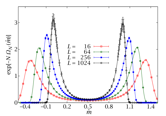
Figure 5.1: Probability density function $p(\hat{m})$ for several lattice sizes at the critical temperature. The peaks get closer as $L$ grows, eventually merging in the thermodynamical limit.

We have used the TMC method, with the simple Metropolis implementation described in Chapter 3, to simulate lattices $L=16,32,\ldots,1024$ at the critical point of the $D=2$ ferromagnetic Ising model. Since the tethered formalism was already constructed using the Ising model as an example, no further notes on it are needed here. However, we still have some practical decisions to make, regarding the numerical implementation:

• We need to decide on a numerical interpolation scheme for the $\braket{O}_{\hat{m}}$ and on a numerical integration method to obtain $\varOmega_{N}$ from $\braket{\hat{b}}_{\hat{m}}$.

• We need to decide which values of $\hat{m}$ to simulate.

These issues are discussed in detail on Appendix C, which also contains some practical recipes for the numerical implementation of the Metropolis algorithm and for the analysis of some delicate physical observables. Suffice it to say here that the issues of interpolation and integration are not critical (all the tethered averages being very smooth functions of $\hat{m}$).

As to the $\hat{m}$ sampling, it is best done starting from a uniform grid and, after a first analysis, perhaps refining the areas that are seen to have more weight in the $p(\hat{m})$. In our case, for systems with $L\leq 256$ we have sampled the $p(\hat{m})$ (see Figure 5.1) with $51$ uniformly distributed points in the interval $\hat{m}\in[-0.5,1.5]$ (except for $L=16$, where the range had to be widened to avoid cutoff errors). For larger lattices the probability density drops much faster at the tails, so we have narrowed the range to $\hat{m}\in[-0.3,1.3]$ and, since the peaks are also steeper, we have then added another $26$ points around the probability maxima (see Section C.2).

In all cases we have performed $10^{7}$ MCS for each value of $\hat{m}$ and computed the errors with $100$ jackknife blocks (see Appendix B for our error estimation techniques), after discarding the first fifth of the measurements for thermalisation (although the correlation times are much smaller, see Section 5.5).

In the following subsection we report the result of computing the canonical expectation values for several standard observables for zero magnetic field. We then demonstrate the new options afforded to us by TMC, by carrying out an unconventional, but very precise, computation of the anomalous dimension of the system from the position of the peak in $p(\hat{m})$. In Section 5.3 we shall reweight these simulations to obtain canonical expectation values at non-zero magnetic field.

5.2.1 Computation of the canonical expectation values

$L$	$-\braket{u}$	$\chi_{2}/L^{2}$	$\xi_{2}/L$	$C$	$B$
$16$ (TMC)	1.453 08(4)	0.545 43(6)	0.911 6(2)	7.718 6(14)	1.165 62(7)
$16$ (CAW)	1.452 9(2)	0.545 1(3)	0.910 4(9)	7.718(10)	1.165 9(3)
$16$ (E)	1.453 065…			7.717 134…
$32$ (TMC)	1.433 69(4)	0.459 00(10)	0.907 2(4)	9.509(3)	1.167 23(14)
$32$ (CSW)	1.433 67(12)	0.459 1(2)	0.907 8(9)	9.493(13)	1.167 1(3)
$32$ (E)	1.433 659…			9.509 379…
$64$ (TMC)	1.423 97(4)	0.386 19(18)	0.906 5(9)	11.285(6)	1.167 5(3)
$64$ (CSW)	1.423 90(6)	0.386 0(2)	0.905 6(10)	11.293(17)	1.167 7(4)
$64$ (E)	1.423 938…			11.288 138…
$128$ (TMC)	1.419 05(5)	0.324 4(3)	0.904 0(18)	13.063(10)	1.168 4(7)
$128$ (CSW)	1.419 06(4)	0.324 59(17)	0.904 8(10)	13.06(2)	1.167 7(4)
$128$ (E)	1.419 076…			13.060 079…
$256$ (TMC)	1.416 63(5)	0.272 8(6)	0.904(4)	14.83(2)	1.168 7(14)
$256$ (CSW)	1.416 64(2)	0.272 86(14)	0.904 2(9)	14.83(2)	1.168 2(4)
$256$ (E)	1.416 645…			14.828 595…
$512$ (TMC)	1.415 42(4)	0.229 3(7)	0.903(6)	16.57(3)	1.168(2)
512 (CSW)	1.415 444(11)	0.229 68(13)	0.905 9(10)	16.60(2)	1.167 6(4)
512 (E)	1.415 429…			16.595 404…
1024 (TMC)	1.414 89(4)	0.194 9(15)	0.919(15)	18.28(8)	1.163(6)
1024 (CSW)	1.414 826(6)	0.193 07(12)	0.904 6(11)	18.35(3)	1.168 1(4)
1024 (E)	1.414 821…			18.361 348…

Table 5.1: Results at the critical temperature and comparison with a cluster algorithm. (TMC): Tethered Monte Carlo, (CSW): Canonical Swendsen-Wang, (E): Exact results at finite $L$ from [ferdinand:69].

Our first physical result is the pdf of $\hat{m}$, represented in Figure 5.1. This distribution features a central minimum in the zero-magnetisation region (recall that $\hat{m}\simeq m+1/2$) as well as two symmetric peaks that get closer together as $L$ grows. Of course, since this system experiences a second-order phase transition, the peaks should converge in the thermodynamical limit (where the effective potential is a convex function).

In Table 5.1 we report our estimates for the canonical expectation values of several standard observables. We check our results against the values obtained from the exact formulas in [ferdinand:69] and against a canonical Swendsen-Wang simulation. We use our own implementation, based on the one distributed with [amit:05], although our results are compatible with those of [salas:00]. We perform $10^{7}$ Swendsen-Wang cluster updates.

From Table 5.1 we can confirm that a simple implementation of TMC is capable of producing very accurate results. The relative errors for $\chi_{2}$ and $B$ scale as $L$. This can be explained by noticing that both are completely determined by $p(\hat{m})$ (see the discussion following Eq. (c.11) in Appendix C). In addition, $\hat{b}$ is self-averaging (cf. Section 2.2.2) and, as we shall see in Section 5.5, virtually free of critical slowing down (meaning that for a fixed simulation length its error scales as $1/\sqrt{N}$). Finally, in the computation of $p(\hat{m})$ we are multiplying $\varOmega_{N}(\hat{m})$ by a factor of $N$, yielding an overall $\sqrt{N}$ scaling for the errors.

Of course, TMC is not meant to be a competitor to cluster algorithms for the Ising model without magnetic field. For example, the CPU time to compute each of the $77$ simulations at fixed $\hat{m}$ for $L=1024$ is similar to what we needed for the whole Swendsen-Wang simulation, which is also more precise. See, however, Chapter 6 for a tethered implementation of the Swendsen-Wang algorithm, which turns out to be as efficient as the canonical Swendsen-Wang for the Ising model. In any case, our tethered version of the Metropolis algorithm is much more efficient than canonical Metropolis (see Section 5.5).

5.2.2 The magnetic critical exponent

Let us now see an example of the new kind of analyses afforded to us by the tethered formalism. In particular, we shall compute the critical parameter $\beta/\nu$ (recall the definitions of the critical exponents in 2.1.2) in a very simple way that, however, would not be practical in a canonical simulation.

We consider the finite-size scaling formula (recall Section 2.1.3)

$$\braket{O}(h)=L^{-y_{O}/\nu}\left[f_{O}(L^{1/\nu}t,L^{y_{h}}h)+\ldots\right],\qquad t=\frac{\beta_{\text{c}}-\beta}{\beta_{\text{c}}}.$$ (5.14)

We have included a second variable in the scaling function $f_{O}$ to allow for displacements in the applied field $h$, not only in temperature. These are regulated by a new critical exponent $y_{h}$ (analogous to $y_{t}=1/\nu$). The dots represent possible corrections to scaling. For the moment, we shall work with no field, $h=0$.

$L$	$-m^{-}_{\mathrm{peak}}=\bigl{|}\hat{m}^{-}_{\text{peak}}-\tfrac{1}{2}\bigr{|}$	$m_{\mathrm{peak}}^{+}=\hat{m}_{\text{peak}}^{+}-\tfrac{1}{2}$
32	0.764 01(10)	0.764 31(11)
64	0.702 86(18)	0.703 0(2)
128	0.645 3(3)	0.645 1(4)
256	0.592 1(7)	0.591 0(7)
512	0.541 9(12)	0.542 7(9)
1024	0.499(2)	0.500(2)

Table 5.2: Position of the positive and negative maxima of the $p(\hat{m})$. Since we are at the critical temperature of a second-order phase transition, both columns should extrapolate to zero in the large-$L$ limit (cf. our study of the ferromagnetic region in Section 5.4).

Applied to the magnetisation, whose associated critical exponent is $\beta$, the FSS ansatz implies that

$$\tilde{p}_{1}(m,\beta_{\mathrm{c}};L)=L^{\beta/\nu}\tilde{f}(L^{\beta/\nu}m),$$ (5.15)

where $\tilde{p}$ is a smooth version of $p_{1}(m;L)$. Now, the pdf of $\hat{m}$, $p(\hat{m};L)$ —Eq. (4.13)— is precisely a smooth version of $p_{1}(\hat{m}-1/2)$. Therefore, we can write

$$p(\hat{m},\beta_{\mathrm{c}};L)=L^{\beta/\nu}f\bigl{(}L^{\beta/\nu}(\hat{m}-1/2)\bigr{)}.$$ (5.16)

If we concentrate on the peaks of the pdf, we see that their height is going to grow as $L^{\beta/\nu}$, while their position is going to shift as

$$|\hat{m}_{\text{peak}}^{\pm}-\frac{1}{2}|\simeq AL^{-\beta/\nu}.$$ (5.17)

Now, computing the maximum of a numerical function is usually a delicate operation. However, in our case we have measured directly $\hat{b}$, which is the derivative of (the logarithm of) $p(\hat{m})$. Herein lies our advantage with respect to a canonical simulation (which cannot access $\hat{b}$ directly), because we only have to find a zero, a much better conditioned operation. In particular, we run through our computed tethered averages $\braket{\hat{b}}_{\hat{m}_{i}}$ until we find two consecutive points in the grid such that $\braket{\hat{b}}_{\hat{m}_{i}}>0$ and $\braket{\hat{b}}_{\hat{m}_{i+1}}<0$. Then, we find the single zero of the section of our cubic spline (see Appendix C) that joins both points. This operation is performed for each jackknife block in order to estimate the statistical error (cf. Appendix B). The resulting maxima are collected in Table 5.2.

Notice that if we just wanted to obtain the maxima very precisely, we would not have performed a simulation of the whole $\hat{m}$ range. Instead, we would have done a fast sweep to place the peaks approximately and then we would have simulated only a few points in their neighbourhood, to a very high precision. However, even with our suboptimal grid we have determined the position of the maxima with a relative ranging from $\sim 10^{-4}$ for $L=32$ to $\sim 5\times 10^{-3}$ for $L=1024$.

$L_{\mathrm{min}}$	$m^{-}_{\mathrm{peak}}$		$m_{\mathrm{peak}}^{+}$
	$\beta/\nu$	$\chi^{2}/\mathrm{d.o.f.}$	$\beta/\nu$	$\chi^{2}/\mathrm{d.o.f.}$
32	0.121 7(3)	23.44/4	0.122 4(3)	27.85/4
64	0.123 9(5)	2.027/3	0.124 5(5)	2.087/3
128	0.125 0(11)	0.7569/2	0.124 6(10)	2.053/2
256	0.126(4)	0.6456/1	0.122 0(23)	0.3248/1

Table 5.3: Fits of $\hat{m}_{\text{peak}}^{\pm}(L)$ to (5.17), in order to find $\beta/\nu$, for different fitting ranges $L\geq L_{\text{min}}$. For each fit we give the chi-square estimator and the degrees of freedom (see Appendix B). Our results converge to the exact value, $\beta/\nu=0.125$.

We have fitted the $\hat{m}_{\text{peak}}^{\pm}$ to (5.17), for different fitting ranges $L\geq L_{\text{min}}$ (Table 5.3). The fits are good (in the sense of an acceptable $\chi^{2}$/d.o.f., see Appendix B) for $L_{\text{min}}\geq 64$. Still, there are possible systematic sources of error (corrections to scaling), so, following [ballesteros:96], we give as our final estimate the fit for $L_{\text{min}}=64$, but with the larger error of the fit for $L_{\text{min}}=128$. For the negative magnetisation peak we find $\beta/\nu=0.123\,9(11)$ and for the positive peak $\beta/\nu=0.124\,5(10)$. Both are compatible with the exact value for the $D=2$ Ising model, known to be $\beta/\nu=1/8$.

Since we have a wide range of lattice sizes, we can try to characterise the first corrections to scaling. Following [salas:00], we assume that in the $D=2$ Ising model the dominant corrections to scaling are analytical

$$m_{\text{peak}}^{\pm}=L^{-\beta/\nu}[A^{\pm}+B^{\pm}L^{-\varDelta}],\qquad\varDelta=7/4.$$ (5.18)

We have fitted our points for all lattices to this expression, fixing the exponents to their exact values and varying $A^{\pm}$ and $B^{\pm}$. We have obtained $\chi^{2}/\text{d.o.f.}=0.9858/4$ for the negative peak and $\chi^{2}/\text{d.o.f.}=2.825/4$ for the positive one.

5.3  Results at $\boldsymbol{\beta}_{\text{c}}$, $\boldsymbol{h}\boldsymbol{\neq}\boldsymbol{0}$

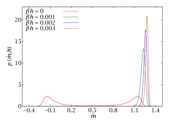
Figure 5.2: Probability density function $p(\hat{m},h)$ for $L=128$ at $\beta_{\text{c}}$, for several values of the applied magnetic field $h$.

One of the strengths of TMC is that it can compute the canonical expectation values for an arbitrary applied field $h$ without any need for new simulations. Notice that in the canonical formalism not only would we have to run a new simulation for each value of $h$, but we would also lose the possibility of using the highly efficient cluster methods. One simply has to change the weight of the tethered expectation values when integrating over $\hat{m}$, as indicated by Eq. (4.23). Figure 5.2 shows an example of this reweighting. We plot the pdf $p(\hat{m};h)$ for several values of the applied field. By integrating the same tethered averages computed in Section 5.2 with this new pdf we can obtain the canonical average at the corresponding applied magnetic field.

Notice that now only a very narrow region has any significant contribution to the canonical average, which implies a loss of statistical precision. In general, if one is interested in the canonical average at a particular value of $h$, the $\hat{m}$ grid should be chosen so that the resulting peak is appropriately sampled, neglecting the exponentially suppressed region away from it. This is a simple task, because the position of the peak is easily determined from a first trial run, as we saw in the previous section. The only difference is that now we do not have to solve for $\braket{\hat{b}}_{\hat{m}}=0$, but for

$$\braket{\hat{b}}_{\hat{m}}=\beta h.$$ (5.19)

Once the peak has been accurately placed, the best strategy is running long tethered simulations precisely there and at neighbouring points.

In this section, however, we are not interested in any particular value of $h$, but rather in studying the behaviour of the canonical averages $\langle{O}\rangle(h)$ as smooth functions of the magnetic field. The simulations we already have will be sufficient, accepting a small loss of precision, because the $\hat{m}$ grid will not be necessarily optimised. We can improve our precision somewhat, though, if we notice that most interesting observables are either odd or even functions of the applied magnetic field. Therefore, we can (anti)symmetrise the curves:

$$\langle O\rangle^{\mathrm{odd}}(h) =\frac{\langle{O}\rangle(h)-\langle{O}\rangle(-h)}{2}\ ,$$ (5.20)

$$\langle O\rangle^{\mathrm{even}}(h) =\frac{\langle{O}\rangle(h)+\langle{O}\rangle(-h)}{2}\ .$$ (5.21)

For statistically independent data, averaging two equivalent estimates in this way would yield an error reduction of $1/\sqrt{2}$. But this is not the case here: the individual averages for $\pm h$ are very strongly correlated. Therefore, the error reduction for even quantities is negligible. For odd quantities, on the other hand, since we are computing a difference, the fluctuations are greatly suppressed and the resulting error reduction is very large (around a factor of $10$, specially for small values of $h$). We shall use equations (5.20) and (5.21), but dropping the explicit ‘odd’ or ‘even’ superscripts.

5.3.1 The magnetisation

We first consider the most straightforward observable, the magnetisation $\langle m\rangle(h)$. This is an odd function of $h$, so as discussed above we can greatly increase our precision by using formula (5.20).

In this case, unlike previous sections, no data for $\langle m\rangle(h)$ are readily available in a finite lattice, since canonical cluster methods lose much of their power in the presence of a magnetic field (in fact, current numerical methods for the investigation of the $D=2$ Ising model in a field typically rely on transfer matrix techniques [caselle:00, grinza:03, caselle:04]). Therefore, rather than compare our results directly with other computations, we shall carry out self-consistency checks.

The first step is recalling Eq. (5.4), according to which the free energy of the system (an even function of $h$, for obvious symmetry considerations) can be written as a Taylor expansion in the following way

$$F_{N}(h)-F_{N}(0)=\sum_{n=1}^{\infty}\frac{\chi_{2n}}{(2n)!}(\beta h)^{2n}\ .$$ (5.22)

Therefore, the magnetisation $\langle{m}\rangle(h)$ is simply

$$\langle m\rangle(h)=\frac{1}{\beta}\frac{\partial F_{N}}{\partial h}=\chi_{2}\ \beta h+\frac{\chi_{4}}{3!}(\beta h)^{3}+\frac{\chi_{6}}{5!}(\beta h)^{5}+\frac{\chi_{8}}{7!}(\beta h)^{7}+\ldots$$ (5.23)

Now, we can compute $\chi_{2n}$ as the cumulants of the magnetisation at $h=0$, but this equation provides an alternative way. We generate a reasonable number of points of the $\langle m\rangle(h)$ curve, which we then parameterise with a truncated version of (5.23). The choice of values for $h$ is somewhat delicate: if we use very small magnetic fields we will only be able to appreciate the first few coefficients but if we go too far in $h$ we would need to have sampled the tails of the pdf of $\hat{m}$ very precisely. We have found that magnetic fields up to $\beta h\sim(\chi_{2})^{-1}$ provide a good compromise (notice that this value is $L$-dependent).

$L$	$N^{-1}\chi_{2}$	$N^{-2}\chi_{4}$	$N^{-3}\chi_{6}$	$N^{-4}\chi_{8}$
16 (M)	0.545 43(6)	$-0.545\,72(13)$	2.265 7(8)	$-20.059(10)$
16  (F)	0.545 43(6)	$-0.545\,7(2)$	2.262 8(19)	$-19.70(14)$
32 (M)	0.459 00(10)	$-0.386\,1(2)$	1.348 5(10)	$-10.042(10)$
32  (F)	0.459 00(10)	$-0.386\,2(3)$	1.348 4(18)	$-10.00(2)$
64 (M)	0.386 19(18)	$-0.273\,3(3)$	0.803 1(13)	$-5.032(11)$
64  (F)	0.386 19(18)	$-0.273\,8(5)$	0.805(2)	$-5.02(2)$
128 (M)	0.324 4(3)	$-0.192\,8(4)$	0.475 8(17)	$-2.504(12)$
128  (F)	0.324 4(3)	$-0.194\,3(7)$	0.481(3)	$-2.52(2)$
256 (M)	0.272 8(6)	$-0.136\,2(7)$	0.283(2)	$-1.250(12)$
256  (F)	0.272 5(6)	$-0.135\,8(15)$	0.280(6)	$-1.20(4)$
512 (M)	0.229 3(7)	$-0.096\,4(7)$	0.168(2)	$-0.625(9)$
512  (F)	0.229 3(7)	$-0.096\,0(12)$	0.166(4)	$-0.60(2)$
1024 (M)	0.194 9(15)	$-0.069\,8(13)$	0.104(3)	$-0.328(12)$
1024  (F)	0.194(3)	$-0.063(6)$	0.08(2)	$-0.2(3)$

Table 5.4: Non-linear susceptibilities from direct measurements at $h=0$ (M) and from a finite-difference formula for $\langle m\rangle(h)$ as a function of the magnetic field (F).

As we discuss in Appendix B, the correlation among the points in the curve has both a beneficial and a detrimental effect. The former is that, since all the points fluctuate more or less coherently, the resulting curves are very smooth. The latter is that these same correlations make it very difficult to estimate errors or to check whether a proposed fitting function is a good model for the data. In this section we have taken the approach of computing an odd interpolating polynomial with a finite-difference formula, which gives us as many $\chi_{2n}$ as we have points. We estimate the statistical errors with the jackknife method. We still face a systematic error, which we try to control by varying both the range in $h$ and the number of points. We have found that the last one or two coefficients in the fit are typically unstable. Therefore, if we want to obtain $n$ physically meaningful parameters, we should compute at least $n+2$ points. In our case, we have computed the non-linear susceptibilities up to $\chi_{8}$, so, to be safe, we have used $7$ points for each lattice size. These were equally spaced at intervals of $\Delta(\beta h)=(10\chi_{2})^{-1}$, where $\chi_{2}$ is the susceptibility computed in the simulation at $h=0$.

In Table 5.4 we compare the non-linear susceptibilities computed from measurements of the cumulants at $h=0$ and from the $\langle m\rangle(h)$ curve. Both series are compatible, but the former are more precise.

We can also perform a FSS analysis. For small applied fields we can collapse the curves for different sizes by plotting $\langle m\rangle(h)/\chi_{2}$ against $\beta h$. As $h$ grows, however, we start to appreciate the deviations from linear behaviour computed above (Figure 5.4—left). We can attempt a better collapse of the curves for different $L$ with the FSS formula (remember Section 5.2.2)

$$\langle m\rangle(h) \simeq L^{-\beta/\nu}f_{m}(L^{y_{h}}h), y_{h}=15/8.$$ (5.24)

We have plotted $\langle m\rangle L^{\beta/\nu}$ against $hL^{y_{h}}$ on Figure 5.4—right. We also include a fit for the scaling function $f_{m}$. We use an odd seventh-degree polynomial and include in the fit the points for $L\geq 64$. The value of the diagonal $\chi^{2}_{\text{d}}$ for this fit is $\chi^{2}_{\text{d}}/\text{d.o.f.}=41.85/31$ (see Appendix B for definitions). The last point in the curve starts to show a deviation, probably due to corrections to leading order scaling. Remember that we spaced our values of $\beta h$ in units of $(10\chi_{2})^{-1}$, which is not an optimal choice for a FSS study.

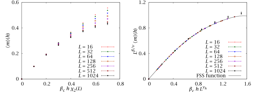
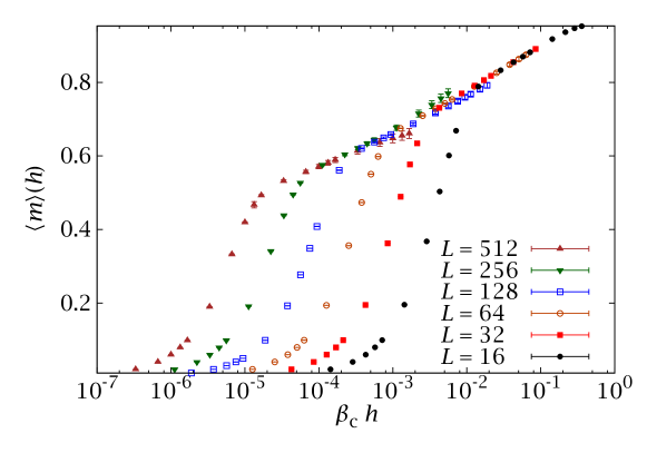
Figure 5.3: Magnetisation as function of the applied magnetic field. In the left panel we have scaled the graphs by the linear susceptibility at zero field, $\chi_{2}(L)$, and appreciate deviations for large fields. In the right panel we show a scaling plot, with a much better collapse. The continuous line is a fit for the scaling function $f_{m}$, Eq. (5.24), using a seventh degree polynomial, with $\chi^{2}_{\mathrm{d}}/\text{d.o.f}=41.85/31$.

Figure 5.4: Magnetisation as a function of the applied field for several lattices at $\beta_{\text{c}}$. We use an $L$-independent range for $h$ (notice the logarithmic scale of the horizontal axis).

We complete our analysis of $\langle m\rangle(h)$ by considering now $L$-independent magnetic fields across several orders of magnitude (Figure 5.4). We observe two well-differentiated scales: a FSS regime, where the slope of the curve is very large, and a saturation regime where the curves merge. Notice that the only hard limit in the values of $h$ we can consider is given by the saddle-point equation (5.19). So long as $\beta h$ is contained within the bounds set by our measured values of $\braket{\hat{b}}_{\hat{m}}$, the peak in $p(\hat{m};h)$ will be contained in our simulated range and we can interpolate it with some precision (this is the reason for the rapid error growth in our largest lattices). Notice that the displacement of the curves in the FSS section seems linear in $\log L$. This is an artifact of the low value of $\beta/\nu=1/8$ in Eq. (5.24).

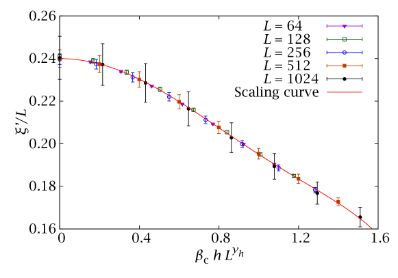
Figure 5.5: Correlation length $\xi^{\prime}(h)/L$, Eq. (5.25), against the scaling variable $\beta_{\text{c}}hL^{y_{h}}$. We also plot a fit to the scaling function $f_{\xi^{\prime}}$ of (5.26).

5.3.2 The correlation length

We consider now the correlation length of the system for non-zero applied field. As we discussed in Section 5.1, the second-moment definition (5.9) does not work in an applied field, so we have to go back to the generic formula (5.8) and choose different $\boldsymbol{k}_{1}$ and $\boldsymbol{k}_{2}$. The simplest choice is to use the next smallest momenta: $\boldsymbol{k}_{1}=\boldsymbol{k}_{\text{min}}$ and $\boldsymbol{k}_{2}=2\uppi/L(1,\pm 1)$,

$$\xi^{\prime}=\frac{1}{2\sin(\uppi/L)}\left[\frac{G_{2}(\boldsymbol{k}_{\text{min}})-G_{2}(\boldsymbol{k}_{2})}{2G_{2}(\boldsymbol{k}_{2})-G_{2}(\boldsymbol{k}_{\text{min}})}\right]^{1/2}\,.$$ (5.25)

Now, $\xi^{\prime}(h)$ is an even function of $h$, so we symmetrise it with (5.21). Again, due to the lack of readily available data in a finite lattice for this observable, we check our results with a FSS analysis. To leading order, we have

$$\xi^{\prime}/L\simeq f_{\xi^{\prime}}(L^{y_{h}}h),$$ (5.26)

where, as in the case of $m$, $f_{\xi^{\prime}}$ is expected to be very smooth. As we can see in Fig. 5.5, Eq. (5.26) is perfectly valid in our case, if we discard the data for $L\leq 32$. At a first glance, it may seem that we have even overestimated our errors for $L=1024$, but remember that the points are very strongly correlated. The universal scaling curve is well represented by a sixth order even polynomial, with $\chi^{2}_{\mathrm{d}}/\text{d.o.f.}=3.978/36$. Thus, the universal scaling function $f_{\xi_{2}}(x)$ for $x\lesssim 1.5$ is very well approximated by

$$f_{\xi^{\prime}}(x)=a_{0}+a_{2}x^{2}+a_{4}x^{4}+a_{6}x^{6},$$ (5.27)

with

$$a_{0} =0.239\,9(2), a_{2} =-0.063\,9(4), a_{4} =0.023\,5(7), a_{6} =-0.004\,5(4).$$ (5.28)

We have estimated the errors in the fit parameters with the techniques of Appendix B.

5.4  The ordered phase: spontaneous symmetry breaking

In this section we present new simulations of the $D=2$ Ising model in the ferromagnetic phase, using them to illustrate the treatment of spontaneous symmetry breaking in the tethered formalism. We then examine the approach to the thermodynamical limit, studying the equivalence between the canonical and tethered ensembles.

5.4.1 Spontaneous symmetry breaking

Let us now consider the $\beta>\beta_{\mathrm{c}}$ regime. In this situation, the infinite system shows a nonzero expectation value for the order parameter, $\langle m\rangle\neq 0$, even in the absence of an external magnetic field, Eq. (5.13). This may seem incompatible with the partition function (4.1), where the configurations $\{s_{\boldsymbol{x}}\}$ and $\{-s_{\boldsymbol{x}}\}$ occur with equal probability. The well-known solution for this apparent paradox is spontaneous symmetry breaking, see, e.g., [huang:87, zinn-justin:05], whose mathematical formulation involves considering a small magnetic field (which establishes a preferred direction) and taking the double limit

$$\langle m\rangle^{(\infty)}=\lim_{h\to 0}\lim_{L\to\infty}\langle m\rangle^{(L)}(h).$$ (5.29)

The order of the two limits is crucial: were we to reverse it, the magnetisation would always vanish. We see then that the symmetry of our model complicates the definition of a broken symmetry phase for finite lattices in the canonical ensemble. The traditional workaround consists in considering not the magnetisation $m$, but its absolute value $|m|$.

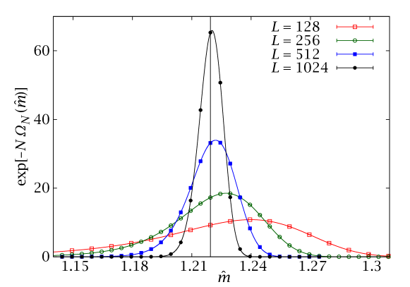
Figure 5.6: Computation at $\beta=0.4473>\beta_{\mathrm{c}}$ (ferromagnetic phase). The peak of the pdf of $\hat{m}$ gets narrower and closer to $m_{\textsc{y}}+1/2$ as $L$ increases (the vertical line, where $m_{\textsc{y}}$ is Yang’s magnetisation for the infinite system at $\beta=0.4473$). Compare the scale of the $OX$ axis and the height of the peaks with those of Fig. 5.1.

$L$	$N_{\mathrm{points}}$	$\Delta\hat{m}$	$-\braket{u}$	$C$	$\xi^{\prime}$	$\braket{m}$
128 (T)	90	0.9	1.490 397(18)	8.874(4)	10.394(17)	0.719 34(6)
128 (E)			1.490 409 763…	8.877 363…
256 (T)	79	0.39	1.490 407(11)	8.869(5)	11.26(4)	0.719 41(4)
256 (E)			1.490 415 672…	8.874 075…
512 (T)	27	0.13	1.490 419(5)	8.877(5)	11.5(3)	0.719 45(3)
512 (E)			1.490 415 689…	8.874 046…
1024 (T)	27	0.13	1.490 416(4)	8.868(7)	11.4(18)	0.719 45(2)
1024 (E)			1.490 415 689…	8.874 046…
$\infty$ (E)			1.490 415 689…	8.874 046…		0.719 436…

Table 5.5: Canonical averages for several physical quantities of an Ising lattice at $\beta=0.4473$ computed with the tethered method (T). The grid of $\hat{m}$ values is uniform in the narrow simulated band. Also included are the exact results for finite lattices from [ferdinand:69] and the exact results in the thermodynamical limit from Eqs. (5.11–5.13). We appreciate that by simulating only a very small range $\Delta\hat{m}$ of values for $\hat{m}$ we can obtain very precise values. Within our error, we have already reached the thermodynamical limit for $L=512$.

The tethered ensemble provides a cleaner concept of broken symmetry phase. Consider the pdf of $\hat{m}$, as in Fig. 5.1. In the ferromagnetic phase the corresponding graph will again have two peaks, but now these will be much narrower and higher, approaching two Dirac deltas in thermodynamic limit. Suppose we want to perform the double limit of equation (5.29). This would involve introducing a small magnetic field which would shift the origin of $\hat{b}$ (4.23). The neighbourhood of one of the peaks would then become exponentially suppressed and eventually disappear in the thermodynamical limit. Thus, we can mimic the effect of equation (5.29) by considering only one of the two peaks from the outset. This would not work at or below $\beta_{\mathrm{c}}$, as there the peaks extrapolate to $m=0$ (recall Section 5.2.2). This procedure has the considerable advantage that it works for any lattice size. In this section we have chosen the peak of positive magnetisation.

We have run simulations for lattice sizes $L=128,256,512,1024$ at inverse temperature $\beta=0.4473>\beta_{\mathrm{c}}$. We chose this temperature as we estimated that the correlation length would be around $\xi^{\prime}\approx 10$.

Following the previous discussion, we have worked in the $\hat{m}>0.5$ (positive magnetisation) region, where there is only one peak. An appropriate sampling of $\hat{m}$ is even more important in this phase (but easier to optimise) than in the situation described in detail in Section C.2. The reason is that the peak is now so narrow that a choice of $\hat{m}$ spaced as in the aforementioned section would not only be completely wasteful, but may also completely fail to sample the peak (remember the loss of precision for very high magnetic fields in Section 5.3).

In the case of the Ising model, we know Yang’s exact solution $m^{\infty}(\beta)$ for the magnetisation of the infinite system, Eq. (5.13). The positive peak for $p(\hat{m})$ will then be very close to $m^{\infty}(\beta)+\tfrac{1}{2}$ and get closer as we increase $L$. With this information in hand, we can adequately reconstruct the effective potential by running simulations in a small neighbourhood of $m^{\infty}(\beta)+\tfrac{1}{2}$. For a different model, where we would lack the knowledge of the peak’s position in the thermodynamical limit, we can just run simulations with a very fine grid for some small and essentially costless lattice size and infer from them an efficient distribution of points for the larger systems.

We have represented $p(\hat{m})$ for all the simulated lattices in Fig. 5.6, which plots the whole simulated range of $\hat{m}$ for $L\geq 512$ (for the smaller lattices we have used a somewhat larger interval). It is interesting to compare the scale on the axes with that of Fig. 5.1. As will be discussed in detail in Section 5.4.2, the peak approaches $m^{\infty}(\beta)+\tfrac{1}{2}$ (the vertical line) as $L$ increases. Table 5.5 compares the values of the energy and specific heat obtained in our simulations with the exact values given in [ferdinand:69]. Notice how very small simulated ranges of $\hat{m}$ ($\Delta\hat{m}=\hat{m}_{\text{max}}-\hat{m}_{\text{min}}$) yield very accurate results. In fact, we can see that for the $L=1024$ lattice we obtain a more precise determination for the energy with $27$ points than what we obtained at the critical temperature with $77$ (we still perform $10^{7}$ Monte Carlo sweeps in each point). This result is even more impressive if we consider that some of these $27$ points, being deeply inside the tails of the distribution, do not have any effect whatsoever in the average with our error (of course, we do not know this until we have run the simulation and seen the actual width of the peak).

From Table 5.5 we can conclude that the thermodynamical limit has already been reached for $L=256$, at least to the level indicated by our errors. Our whole computation for $L=512$ required about $270$ hours of computer time. For comparison, a Swendsen-Wang computation with a run time of $30$ hours for $L=512$ gives $\xi^{\prime}=11.8(2)$. We see that the ratio of computation time for both methods has changed significantly from the critical point, where the advantage of the cluster algorithm was much greater.

5.4.2 Ensemble equivalence

Once we wander away from the critical point, the main goal is finding the value of physical quantities in the thermodynamical limit, rather than attempting a finite-size scaling. The ensemble equivalence property discussed in Section 4.2 suggests a way to reach this limit without constructing the whole canonical $p(\hat{m})$, but by concentrating instead on its maximum. From the computational point of view, this supposes a dramatic reduction in the needed effort for a TMC simulation.

Ensemble equivalence can be expressed in mathematical terms by

$$\lim_{N\to\infty}\braket{O}=\lim_{N\to\infty}\braket{O}_{\hat{m}_{\text{peak}}},$$ (5.30)

where $\hat{m}_{\text{peak}}$ is the saddle point of Section 4.2 (for zero field, in this case). This equation can be understood as a more formal way of summarising the behaviour of Fig. 5.6. Indeed, we saw in the previous section that we could reconstruct the canonical averages considering only a very narrow range of $\hat{m}$; in the thermodynamic limit a single point would be sufficient.

For the Ising model we know exactly where this point would be situated, because, from Yang’s spontaneous magnetisation (5.13)

$$\hat{m}^{\infty}(\beta)=\lim_{N\to\infty}\braket{m}+\frac{1}{2}=\left[1-(\sinh 2\beta)^{-4}\right]^{1/8}+\frac{1}{2}.$$ (5.31)

We could then run simulations for several lattice sizes precisely at $\hat{m}^{\infty}$ and study the evolution of $\braket{O}_{\hat{m}^{\infty}}$ as we increase $L$. This is not the most practical approach, as for a model other than the $D=2$ Ising lattice we would not know the position of the peak beforehand. Instead, we will follow a more general analysis that would work in more complex situations.

Let us consider the canonical average of some quantity and recall that we are using periodic boundary conditions, so the approach to the thermodynamical limit is exponential

$$\braket{O}=\int_{1/2}^{\infty}\mathrm{d}\hat{m}\ p(\hat{m},\beta;L)\braket{O}_{\hat{m}}=O^{\infty}+A_{O}\mathrm{e}^{-L/\xi_{\infty}},$$ (5.32)

where $A_{O}$ is a constant amplitude. We have just considered the positive magnetisation peak.

$L$	$\beta=0.4473$
	$\hat{b}^{\infty}\cdot 10^{5}$	$\hat{m}_{\mathrm{peak}}^{+}$	$-u_{\mathrm{peak}}^{+}$
16	$2984(3)$	1.343 84(4)	1.577 07(8)
32	$924.7(16)$	1.299 30(7)	1.528 98(9)
64	$284.9(9)$	1.263 33(7)	1.505 48(5)
128	$86.0(6)$	1.239 88(9)	1.495 63(4)
256	$25.5(3)$	1.227 32(8)	1.491 99(2)
512	$6.9(2)$	1.222 04(6)	1.490 859(16)
1024	$2.11(11)$	1.220 24(4)	1.490 538(9)
$\infty$	0	1.219 435…	1.490 416…

$L$	$\beta=0.6$
	$\hat{b}^{\infty}\cdot 10^{5}$	$\hat{m}_{\mathrm{peak}}^{+}$	$-u_{\mathrm{peak}}^{+}$
16	$-290.6(14)$	1.471 943(7)	1.912 98(4)
32	$-52.5(8)$	1.473 299(5)	1.910 18(2)
64	$-11.0(4)$	1.473 543(2)	1.909 374(9)
128	$-2.45(19)$	1.473 594 0(12)	1.909 165(5)
256	$-0.67(11)$	1.473 604 7(2)	1.909 107(3)
512	$-0.19(5)$	1.473 607 7(4)	1.909 090 7(15)
1024	$-0.03(2)$	1.473 608 3(2)	1.909 086 7(4)
$\infty$	0	1.473 608 7…	1.909 086 2…

Table 5.6: Tethered mean values of several parameters at the peak of the probability density function for $\beta=0.4473$ and $\beta=0.6$, together with the value of $\hat{b}^{\infty}=\braket{\hat{b}}_{\hat{m}^{\infty}}$ (this observable is zero at the peak and helps characterise how close we are to it). The exact value for an infinite lattice, which coincides with the canonical average, is also included for comparison.

The integral will be dominated by a saddle point at $\hat{m}_{\text{peak}}^{+}$, with $\hat{m}_{\text{peak}}^{+}\xrightarrow{L\to\infty}\hat{m}^{\infty}$, so we can approximate the pdf by a Gaussian

$$p(\hat{m},\beta;L)\simeq\sqrt{\frac{N}{2\uppi\chi_{2}}}\exp\left[-\frac{N(\hat{m}-\hat{m}_{\text{peak}})^{2}}{2\chi_{2}}\right].$$ (5.33)

Therefore, we expect the tethered average of $O$ at this saddle point to approach the canonical average (5.32), with a correction of order $N^{-1}$,

$$O^{\infty}=\braket{O}-A_{O}\mathrm{e}^{-L/\xi_{\infty}}=\braket{O}_{\hat{m}_{\text{peak}}^{+}}+\mathcal{O}\left(L^{-D}\right).$$ (5.34)

To ease the notation we shall use the definition

$$O^{+}_{\text{peak}}=\braket{O}_{\hat{m}_{\text{peak}}^{+}}.$$ (5.35)

This simple analysis provides a practical way of approaching the thermodynamic limit without knowing the limiting position of the peak in advance.

We first run a complete simulation for some small lattice, covering the whole range of $\hat{m}$. This provides a first approximation to the position of the peak. For growing lattices, we just compute two or three points at both sides of where we think the maximum is going to be. Our objective is not to reconstruct the whole peak of $p(\hat{m})$, just to find a good approximation to the point $\hat{m}_{\text{peak}}^{+}$ where $\braket{\hat{b}}_{\hat{m}}$ vanishes. We use the same procedure as in Section 5.2.2, finding the zero of the cubic spline and interpolating the physical observables. Actually, if the position of the peak is sufficiently bounded we could just place one point very closely at either side and use a linear interpolation.

With this procedure we are able to compute the tethered mean values of the relevant physical quantities at the peak with a minimum of numerical effort. Here we shall apply this method to the energy and we shall also characterise the approach of the peak to $\hat{m}^{\infty}$. To the latter purpose, we have computed $\hat{b}^{\infty}=\braket{\hat{b}}_{\hat{m}^{\infty}}$ for several lattice sizes and studied how fast it approaches zero. We also give the values for the position of the peak (Table 5.6).

Following the above analysis we should find that

$$|u^{+}_{\text{peak}}-u^{\infty}| =A_{u}\cdot L^{-\zeta_{u}},$$

$$|\hat{m}^{+}_{\text{peak},\beta}-\hat{m}^{\infty}| =A_{\hat{m}}\cdot L^{-\zeta_{\hat{m}}},$$ (5.36)

$$\hat{b}^{\infty} =A_{\hat{b}}\cdot L^{-\zeta_{\hat{b}}},$$

with $\zeta\approx 2$. We present in Table 5.7 the result of applying the quotients method (see Section 8.5) to these observables. As we can see, our results are always $\zeta<2$, even though this exponent grows with $L$.

We believe this was caused by the proximity of the critical point, so we ran analogous simulations for $\beta=0.6$. We were able to complete this new computations in very little time, following the above procedure. For example, for $L=512$ the position of the peak was so tightly bounded that we just computed one point at either side.

$L$	$\beta=0.4473$			$\beta=0.6$
	$\zeta_{\hat{b}}$	$\zeta_{\hat{m}}$	$\zeta_{u}$	$\zeta_{\hat{b}}$	$\zeta_{\hat{m}}$	$\zeta_{u}$
16	1.690(3)	0.6394(14)	1.168(4)	2.47(2)	2.43(2)	1.83(3)
32	1.699(5)	0.864(3)	1.356(6)	2.25(5)	2.24(5)	1.93(5)
64	1.729(12)	1.102(7)	1.531(12)	2.17(12)	2.16(13)	1.87(10)
128	1.75(2)	1.375(16)	1.73(3)	1.9(3)	1.89(13)	1.9(2)
256	1.88(5)	1.60(4)	1.83(6)	1.8(4)	2.0(5)	2.2(5)
512	1.71(9)	1.70(8)	1.85(12)	2.7(12)	1.4(10)	3.1(12)

Table 5.7: Rate at which several observables approach zero. We consider a functional form $A\cdot L^{-\zeta}$ and compute the effective exponent $\zeta$ from the ratio of the computed values at consecutive lattice sizes. We consider three exponents, $\zeta_{\hat{b}}$, $\zeta_{\hat{m}}$ and $\zeta_{u}$ for the evolution of $\hat{b}^{\infty}$, $\hat{m}_{\text{peak}}^{+}$ and $u^{+}_{\text{peak}}$, respectively, see (5.36). We observe that for $\beta=0.6$ the effective exponent approaches $2$, as expected from the discussion in the text, while for $\beta=0.4473$ the proximity of the critical point complicates the analysis.

Comparing Table 5.6 with Table 5.1 we see that for $\beta=0.6$, with a computation effort almost $40$ times smaller, we have obtained a result an order of magnitude more precise than what we had at $\beta_{\mathrm{c}}$. Recomputing the effective exponents for these new simulations we obtain results compatible with $\zeta=2$. Notice that for this temperature the error in the exponents is much bigger than that for $\beta=0.4473$. The reason is clear from Table 5.6. The left-hand sides of (5.36) are now much closer to zero than in $\beta=0.4473$, yet their errors are only slightly smaller. In the computation of the effective exponents only the relative errors matter, which explains our bigger uncertainties. Notice, however, that we have been able to distinguish values for $b^{\infty}$ of order $10^{-6}$ from zero and that we have located the peak with seven significant figures.

5.5  Numerical performance analysis

We consider here the Metropolis update algorithm described in detail in Section 3.2.1, for a $D=2$ Ising model at the critical temperature. Notice that, since this is a local update algorithm, one would expect the autocorrelation times (see Appendix A for definitions) to scale as

$$\tau\propto L^{z}$$ (5.37)

with $z\approx 2$, due to critical slowing down [hohenberg:77, zinn-justin:05].

$L$	$\ \hat{m}=0.5$	$\hat{m}=1.14$
32	0.491(9)	0.564(4)
64	0.548(11)	0.614(8)
128	0.580(14)	0.654(8)
256	0.597(13)	0.641(6)
512	0.639(4)	0.661(4)
1024	0.632(4)	0.665(5)

Table 5.8: Autocorrelation times for the tethered magnetic field $\langle\hat{b}\rangle_{\hat{m}}$ at the minimum, $\hat{m}=0.5$, and close to one of the maxima of the $p(\hat{m})$ for a critical $D=2$ Ising model, simulated with a Metropolis algorithm. There is no critical slowing down for this observable. The times appear to grow for small sizes, but this is an artificial effect of the discrete nature of Monte Carlo time (notice that $\tau\geq 1/2$ by construction and that times very close to this limit are difficult to measure).

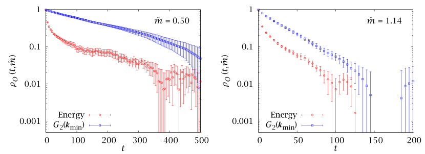
Figure 5.7: Normalised autocorrelation functions $\rho_{O}(t,\hat{m})$ for the energy and the propagator $G_{2}({\boldsymbol{k}}_{\text{min}})$ at $T_{\text{c}}$ in an $L=128$ lattice. We plot them at the central minimum of $p(\hat{m})$ (left) and at one of the peaks (right). In both cases, the correlation function for $G_{2}$ is almost a pure exponential. Notice, however, that the correlation functions for both quantities become parallel, indicating that they share the same exponential autocorrelation time.

In Table 5.8 we show the integrated autocorrelation times for the tethered magnetic field at the values of the smooth magnetisation $\hat{m}$ corresponding to the minimum and one of the maxima in $p(\hat{m})$ (recall Figure 5.1). As we can see, there is hardly any evolution (in fact, the values are so small that we cannot even measure them properly, since times smaller than one are meaningless in a sequential update scheme). The same situation is reproduced if we consider the autocorrelation times for other magnetic observables (functions of the magnetisation $m$). This result is surprising, specially considering that naive conserved order parameter dynamics exhibit $z=4-\eta$ critical slowing down [hohenberg:77].

The key is that our method imposes the constraint globally so, even though the update algorithm is local, the magnetisation has global information. In this case, the new dynamical exponent should be $z_{\text{nonlocal}}=z-2\approx 0$ [tamayo:89], as is the case for our method. Notice that this result implies that Tethered Monte Carlo is able to reconstruct the effective potential $\varOmega_{N}$ without critical slowing down for the Ising model.

Other physical observables, however, do not enjoy the same nonlocal information as $\hat{b}$ and therefore show standard critical slowing down. This is the case, for instance, of the energy. The quantity with the slowest dynamics seems to be to be the two-point propagator $G_{2}$, defined in (5.5), We have plotted in Figure 5.7 the temporal autocorrelation for the energy and for $G_{2}$ in an $L=128$ lattice, at the central probability minimum and at the probability peak. At both magnetisations, the correlation functions for the energy and propagator become parallel for long enough times. This indicates that they both have the same exponential time, which we also expect to be the exponential time of the system as a whole. In addition, the $\rho_{g_{2}}(t,\hat{m})$ is almost a pure exponential, so we can make the approximation

$$\tau_{\text{exp}}=\tau_{\text{exp},G_{2}}\simeq\tau_{\text{int},G_{2}}\,.$$ (5.38)

Figure 5.8 shows this exponential time as a function of $\hat{m}$ for several system sizes. As we can see, the central region does exhibit critical slowing down. Notice, however, that even for an $L=1024$ system $\tau_{\text{exp}}$ is only $\sim 10^{4}$, so this simple Metropolis algorithm can be used safely to study very large systems. As a comparison, the exponential autocorrelation time of the canonical version of the Metropolis algorithm for $L=64$ is already as large as that of the tethered version for $L=1024$ (see, e.g., [amit:05]).

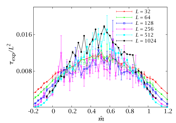
Figure 5.8: Exponential autocorrelation times for tethered simulations of the $D=2$ Ising model at the critical point, as a function of $\hat{m}$. The $\tau_{\text{exp}}$, computed from the correlation function of $G_{2}({\boldsymbol{k}}_{\text{min}})$, are represented in units of the system size, showing a $z\approx 2$ critical slowing down.

CHAPTER VI   Optimising Tethered Monte Carlo: cluster methods

In the previous chapter we showed how a straightforward implementation of the tethered formalism, using as Monte Carlo dynamics the simple Metropolis algorithm, can be very precise and efficient. Eventually, however, the system size we can consider in the critical regime is capped by the appearance of critical slowing down, according to which the thermalisation times grow as $\tau\sim L^{z}$, with $z\approx 2$.

However, this $z\approx 2$ is not a hard limit imposed by the tethered formalism, but is instead determined by the Metropolis algorithm we have used to explore the tethered ensemble. If we had run our tethered simulations with some kind of optimised dynamics, the critical slowing down would have been reduced. In this chapter we consider the most spectacular example of optimised update algorithm: cluster methods. These are able to achieve $z<1$, for all intents and purposes eliminating critical slowing down. Because of this, since their introduction in the 1980s [swendsen:87, wolff:89], they have attracted a considerable interest, which lasts to the present day [chayes:98, deng:07c, deng:07d, deng:07, deng:07b, deng:10, garoni:11]. Despite this continued research effort, however, efficient implementations of cluster methods remain restricted to very few situations. In particular, the development of a cluster update algorithm with conserved order parameter dynamics has long been considered somewhat of a challenge [annett:92].

The work reported in this chapter (whose results were originally published, in a reduced form, in [martin-mayor:09]) shows how, using the tethered formalism, one can actually define a workable cluster update with a conserved order parameter. This is demonstrated in the context of the $D=2,3$ ferromagnetic Ising model, the ideal scenario for canonical cluster methods. Furthermore, the tethered version of the cluster update is shown to be just as efficient (in the sense of having the same $z$ exponent) as the canonical one.

6.1  The canonical Swendsen-Wang algorithm

We summarise here the construction of the Swendsen-Wang algorithm, following [edwards:88]. The process is based on the Fortuin-Kasteleyn transformation [kasteleyn:69, fortuin:72], which maps Potts models onto bond-percolation problems. We start by rewriting the partition function of the Ising model in the following way

$$Z =\sum_{\{s_{\boldsymbol{x}}\}}\exp\biggl{[}\beta\sum_{\braket{{\boldsymbol{x}},{\boldsymbol{y}}}}s_{\boldsymbol{x}}s_{\boldsymbol{y}}\biggr{]}=\mathrm{e}^{\beta}\sum_{\{s_{\boldsymbol{x}}\}}\prod_{\braket{{\boldsymbol{x}},{\boldsymbol{y}}}}\bigl{[}p\delta_{s_{\boldsymbol{x}},s_{\boldsymbol{y}}}+(1-p)\bigr{]},$$ (6.1)

where

$$p=1-\mathrm{e}^{-2\beta}.$$ (6.2)

We now notice that, trivially,

$$\bigl{[}p\delta_{s_{\boldsymbol{x}},s_{\boldsymbol{y}}}+(1-p)\bigr{]}=\sum_{n=0,1}\bigl{[}p\delta_{s_{\boldsymbol{x}},s_{\boldsymbol{y}}}\delta_{n,1}+(1-p)\delta_{n,0}\bigr{]}.$$ (6.3)

Finally, we introduce this identity in the partition function by considering one auxiliary variable $n_{{\boldsymbol{x}}{\boldsymbol{y}}}$ for each first-neighbours pair $\braket{{\boldsymbol{x}},{\boldsymbol{y}}}$:

$$Z =\sum_{\{s_{\boldsymbol{x}}\}}\sum_{\{n_{{\boldsymbol{x}}{\boldsymbol{y}}}\}}\prod_{\braket{{\boldsymbol{x}},{\boldsymbol{y}}}}\bigl{[}p\delta_{s_{\boldsymbol{x}},s_{\boldsymbol{y}}}\delta_{n_{{\boldsymbol{x}}{\boldsymbol{y}}},1}+(1-p)\delta_{n_{{\boldsymbol{x}}{\boldsymbol{y}}},0}\bigr{]}.$$ (6.4)

This partition function describes a model with $(D+1)N$ dynamic variables: the original $N$ spins of the Ising model and the $DN$ auxiliary variables $n_{{\boldsymbol{x}}{\boldsymbol{y}}}$. We can think of the latter as bond-occupation variables. We say that a link ${\boldsymbol{x}}{\boldsymbol{y}}$ is occupied if $n_{{\boldsymbol{x}}{\boldsymbol{y}}}=1$ and that it is empty if $n_{{\boldsymbol{x}}{\boldsymbol{y}}}=0$. Notice that the spins joined by an occupied bond must be aligned, while those joined by an empty bond can be either aligned or opposed. Therefore, the system has been partitioned into several clusters (two spins are in the same cluster if they can be connected by a path of occupied bonds).

If we sum over the $s_{\boldsymbol{x}}$ for fixed bonds, we see that, while all spins in the same cluster must be aligned, the orientation of separate clusters is independent. Consider a bond configuration with $\ell$ occupied bonds, defining ${\mathcal{N}}_{\text{C}}$ clusters (some of which may be single-spin clusters). We see in (6.4) that each occupied bond contributes a factor $p$ to the weight and that each empty one contributes a factor $(1-p)$. There are $2^{{\mathcal{N}}_{\text{C}}}$ possible cluster orientations. Therefore, the marginal probability of the bonds is just

$$\omega(\{n_{{\boldsymbol{x}}{\boldsymbol{y}}}\})=Z^{-1}p^{\ell}(1-p)^{DN-\ell}2^{{\mathcal{N}}_{\text{C}}}.$$ (6.5)

More interesting are the conditioned probabilities of the spins given the bonds and vice versa, which can be read directly from (6.4),

• Given the $\{s_{\boldsymbol{x}}\}$, the bonds are independent from one another and $n_{{\boldsymbol{x}}{\boldsymbol{y}}}=1$ with probability $p\delta_{s_{{\boldsymbol{x}}},s_{\boldsymbol{y}}}$ and $n_{{\boldsymbol{x}}{\boldsymbol{y}}}=0$ otherwise.

• Given the $\{n_{{\boldsymbol{x}}{\boldsymbol{y}}}\}$, all the spins within a cluster are aligned and two spins in different clusters are independent from each other. Each cluster has a positive or negative orientation with $50\%$ probability.

These conditioned probabilities can be used to define a Monte Carlo update scheme. Each lattice update consists of two steps:

1. Given a starting spin configuration $\{s_{\boldsymbol{x}}\}$, the conditioned probability $(a)$ is used to trace the clusters. This can be implemented in several ways, with an algorithmic complexity of $\mathcal{O}(N\log N)$. See [landau:05] or the code distributed with [amit:05] for an example.

2. Once the clusters are traced, they must be flipped to update the spin configuration. The conditioned probability $(b)$ is trivial, the sign of each cluster is chosen as $\pm 1$ with $50\%$ probability.

Each of these two steps satisfies the detailed balance condition. The combination of the two is irreducible and satisfies balance (see Section A.1 for definitions).

This scheme can be implemented for systems other than the Ising model (for instance, in an antiferromagnetic model, the clusters have uniform staggered magnetisation), but it is for this system that it shows its full power. The critical slowing down is practically eliminated, with $z<1$ in both two and three dimensions (see below), meaning that even for very large lattices a few updates are enough to decorrelate the system completely.

6.1.1 Improved estimators

Performing a single cluster update changes the spin configuration radically, almost instantaneously decorrelating the system. Therefore, not only is the system thermalised very quickly, but one can also take measurements very frequently and obtain independent data (remember the discussion of integrated and exponential correlation times in Appendix A).

But the statistical gain of a cluster scheme does not end here. Indeed, in the Swendsen-Wang scheme, after tracing the clusters, we have to flip them randomly, and with equal probability for each orientation, in order to obtain our new system configuration. However, when taking measurements of some physical observables we can consider at once the average over all the $2^{{\mathcal{N}}_{\text{C}}}$ possible cluster orientations with fixed $\{n_{{\boldsymbol{x}}{\boldsymbol{y}}}\}$. We obtain in this way the so-called improved or cluster estimators [sweeny:83, wolff:88].

Let us call $S_{i}=\pm 1$ the spin of the $i$-th cluster and $n_{i}$ its size. Then, the spin estimator for the magnetisation of the system is

$$M=\sum_{{\boldsymbol{x}}}s_{\boldsymbol{x}}=\sum_{i}n_{i}S_{i}.$$ (6.6)

And the squared magnetisation is

$$M^{2}=\sum_{{\boldsymbol{x}}{\boldsymbol{y}}}s_{\boldsymbol{x}}s_{\boldsymbol{y}}=\sum_{i,j}n_{i}n_{j}S_{i}S_{j}.$$ (6.7)

Let us denote by an overbar the average over the $2^{N_{\text{C}}}$ cluster configurations $\{S_{i}\}$. Obviously,

$$\overline{M}=\sum_{i}n_{i}\overline{S}_{i}=0.$$ (6.8)

For the squared magnetisation, only the diagonal terms survive (remember the $S_{i}$ are independent)

$$\overline{M^{2}}=\sum_{i}n_{i}^{2}\overline{S_{i}^{2}}=\sum_{i}n_{i}^{2}.$$ (6.9)

Obviously, $\braket{M^{2}}=\braket{\overline{M^{2}}}$, but the second estimator has more information and is therefore potentially more precise. We can do the same for other observables, for instance,

$$\overline{M^{4}} =3\sum_{i,j}n_{i}^{2}n_{j}^{2}-2\sum_{i}n_{i}^{4},$$ (6.10a)

$$\overline{M^{6}} =15\sum_{i,j,k}n_{i}^{2}n_{j}^{2}n_{k}^{2}-30\sum_{i,j}n_{i}^{2}n_{j}^{4}+16\sum_{i}n_{i}^{6},$$ (6.10b)

$$\overline{M^{8}} =105\sum_{i,j,k,l}n_{i}^{2}n_{j}^{2}n_{k}^{2}n_{l}^{2}-420\sum_{i,j,k}n_{i}^{2}n_{j}^{2}n_{k}^{4}+448\sum_{i,j}n_{i}^{2}n_{j}^{6}$$

$$\qquad+140\sum_{i,j}n_{i}^{4}n_{j}^{4}-272\sum_{i}n_{i}^{8}.$$ (6.10c)

Consider now the propagator $G_{2}(\boldsymbol{k})$, Eq. (5.5), with spin estimator for a given configuration

$$G_{2}(\boldsymbol{k})=\left|\sum_{\boldsymbol{x}}s_{\boldsymbol{x}}\mathrm{e}^{\mathrm{i}\boldsymbol{k}\cdot{\boldsymbol{x}}}\right|^{2}=\sum_{{\boldsymbol{x}}{\boldsymbol{y}}}s_{\boldsymbol{x}}s_{\boldsymbol{y}}\mathrm{e}^{\mathrm{i}\boldsymbol{k}\cdot{\boldsymbol{x}}}\mathrm{e}^{-\mathrm{i}\boldsymbol{k}\cdot{\boldsymbol{y}}}.$$ (6.11)

Now, when averaging over the cluster orientations at fixed $\{n_{{\boldsymbol{x}}{\boldsymbol{y}}}\}$, two spins belonging to different clusters are uncorrelated and two spins in the same cluster are equal, therefore

$$\overline{G_{2}(\boldsymbol{k})}=\sum_{i=1}^{{\mathcal{N}}_{\text{C}}}\left|\sum_{{\boldsymbol{x}}\in C_{i}}\mathrm{e}^{\mathrm{i}\boldsymbol{k}\cdot{\boldsymbol{x}}}\right|^{2}\,.$$ (6.12)

The error reduction due to the adoption of cluster estimators is heavily dependent on the cluster distribution (see [fernandez:09c]), but it can be very large. See, for instance, Table 6.1, where we compute the renormalised coupling constants of the $D=2$ Ising model with several methods, and obtain a tenfold error reduction using cluster estimators.

$O$	TMC	SWS	SWC
$-\braket{u}$	1.226 067(7)	1.226 076(8)
$\chi_{2}$	203.78(11)	204.07(10)	203.92(2)
$\xi_{2}$	11.888(11)	11.907(10)	11.893 2(10)
$r_{6}$	3.70(6)	3.73(8)	3.731(6)
$r_{8}$	26.2(6)	24(3)	26.47(18)
$g_{4}$	14.66(5)	14.69(9)	14.673(8)
$g_{6}$	794(9)	806(24)	803.3(16)
$g_{8}/10^{4}$	8.25(13)	7.5(11)	8.34(7)

Table 6.1: Several observables for the $D=2$ Ising model (the $r_{i}$ and $g_{i}$ are renormalised coupling constants, see [caselle:01] for definitions). We work at $\beta=0.42$, with $L=100$, and take $10^{8}$ Swendsen-Wang lattice updates. Compare the results with spin estimators (SWS) and with cluster estimators (SWC). We also give, for comparison, results with the Metropolis TMC algorithm ($191$ values of $\hat{m}$, with $10^{7}$ MCS on each).

6.2  The tethered Swendsen-Wang algorithm

The Fortuin-Kasteleyn construction is just as easy to do in the tethered formalism. Remember the tethered weight

$$\omega_{N}(\hat{m},\{s_{\boldsymbol{x}}\})\propto\mathrm{e}^{-\beta U+M-\hat{M}}(\hat{m}-m)^{(N-2)/2}\varTheta(\hat{m}-m).$$ (4.17)

Notice that the spin-connectivity term, given by the energy $U$, is exactly the same as that of the canonical weight $\omega_{\text{canonical}}=\exp[-\beta U]$, and can thus be represented as in (6.4). Therefore, the conditioned probability of the bonds given the spins is exactly the same in the tethered and the canonical ensembles. Only the conditioned probability of the spins given the bond varies,

• Given the $\{s_{\boldsymbol{x}}\}$, the bonds are independent from one another and $n_{{\boldsymbol{x}}{\boldsymbol{y}}}=1$ with probability $p\delta_{s_{{\boldsymbol{x}}},s_{\boldsymbol{y}}}$ and $n_{{\boldsymbol{x}}{\boldsymbol{y}}}=0$ otherwise.

• Given the $\{n_{{\boldsymbol{x}}{\boldsymbol{y}}}\}$, all the spins within a cluster are aligned and two spins in different clusters are independent from each other. Each of the $2^{{\mathcal{N}}_{\text{C}}}$ cluster configurations $\{S_{i}\}$ has probability

  $$p(\{S_{i}\})\propto\mathrm{e}^{M-\hat{M}}(\hat{m}-m)^{(N-2)/2}\varTheta(\hat{m}-m),\qquad M=Nm=\sum_{i}n_{i}S_{i}.$$ (6.13)

Just as in the canonical case, the tethered Swendsen-Wang lattice update has two steps. First we trace the clusters using the conditioned probability $(a)$. Then we flip them using $(b^{\prime})$. This second step was trivial in the canonical ensemble, as all $2^{{\mathcal{N}}_{\text{C}}}$ cluster configurations were equiprobable. In the tethered ensemble, however, we have to pick one using (6.13). A naive way to make this choice would be to select one configuration randomly and accept it with a heat-bath probability,

$$P=\frac{p(\{S_{i}\})}{\sum_{j=1}^{{\mathcal{N}}_{\text{C}}}p(\{S_{j}\})}\ .$$ (6.14)

The problem with this method is obvious: ${\mathcal{N}}_{\text{C}}$ is potentially a very large number, so it is impossible to compute all the weights and average them.

Clearly, we need a more manageable scheme. In order to construct it let us first recall the Wolff or single-cluster algorithm [wolff:89]. With this (canonical) method, we randomly pick one spin and immediately trace and flip the cluster to which it belongs. Since the clusters are flipped with probability proportional to their size, this method is able to cause a very large change in the system.

In the tethered formalism we cannot take the same approach, because the weights of the configurations with $\pm S_{i}$ are different. We can, however, make use of the notion that not all clusters need be flipped. Indeed, we can select ${\mathcal{N}}^{\prime}_{\text{C}}\ll{\mathcal{N}}_{\text{C}}$ clusters and consider a heat bath of the $2^{{\mathcal{N}}^{\prime}_{\text{C}}}$ configurations $\{S^{\prime}_{i}\}$ where all the other clusters are fixed. In principle, one could select one of the $\{S^{\prime}_{i}\}$ randomly and accept it with probability

$$P^{\prime}=\frac{p(\{S^{\prime}_{i}\})}{\sum_{j=1}^{{\mathcal{N}}^{\prime}_{\text{C}}}p(\{S^{\prime}_{j}\})}\ .$$ (6.15)

This is already a manageable computation, but there still remains a problem. Since the weight (6.13) is heavily dependent on $M$, only a few of the $2^{{\mathcal{N}}^{\prime}_{\text{C}}}$ configurations will have non-negligible weight. Therefore, a method where we choose one randomly and check whether it is accepted with (6.15) is going to have a very low acceptance. It is better to use a modified representation of the heat bath algorithm, where we construct a vector with the cumulative probabilities

$$A_{k}=\frac{\sum_{j=1}^{k}p(\{S^{\prime}_{j}\})}{\sum_{j=1}^{{\mathcal{N}}^{\prime}_{\text{C}}}p(\{S^{\prime}_{j}\})},\qquad A_{0}=0.$$ (6.16)

We then extract a uniform random number $0\leq\mathcal{R}<1$ and choose the configuration $\{S^{\prime}_{k}\}$ such that

$$A_{k-1}\leq\mathcal{R}<A_{k}.$$ (6.17)

We still have to decide how to choose the ${\mathcal{N}}^{\prime}_{\text{C}}$ clusters that we will attempt to flip. Two simple choices, both satisfying the balance condition, present themselves:

• Select the ${\mathcal{N}}^{\prime}_{\text{C}}$ largest clusters.

• Select ${\mathcal{N}}^{\prime}_{\text{C}}$ spins randomly and note their clusters (in case of repetition, we keep drawing spins until we get ${\mathcal{N}}^{\prime}_{\text{C}}$ different clusters).

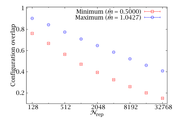
Figure 6.1: Spin overlap, Eq. (6.18), in a $D=2$ critical $L=512$ Ising model. We plot the results, whose errors cannot be discerned at this scale, for the central minimum of the $p(\hat{m})$ and for one of its maxima.

It may seem that the first choice is preferable, with more potential for changing the system quickly. However, nothing says that we can only select the ${\mathcal{N}}^{\prime}_{\text{C}}$ clusters and flip them once, before retracing the clusters. In fact, tracing the clusters is a relatively costly operation, $\mathcal{O}(N\log N)$, so the flipping time is negligible. Therefore, we can adopt the following algorithm as our lattice update

1. Trace the clusters in the system.

2. Flip the clusters. For $t=1,\ldots,{\mathcal{N}}_{\text{rep}}$ do

   1. Select ${\mathcal{N}}^{\prime}_{\text{C}}$ clusters with the second of the methods described above (we use ${\mathcal{N}}^{\prime}_{\text{C}}=5$, but this number can be changed).

   2. Obtain the $\{S_{i}^{t}\}$ with the heat bath of Eq. (6.16), fixing the ${\mathcal{N}}_{\text{C}}-{\mathcal{N}}_{\text{C}}^{\prime}$ remaining clusters in the orientations they had at $t-1$.

We are therefore using a dynamic Monte Carlo in order to pick the cluster orientations, rather than a static Monte Carlo, as is the case for the canonical algorithm. It may seem counterintuitive that the optimal value of ${\mathcal{N}}_{\text{rep}}$ is rather large. In order to see it, let us consider the overlap

$$o=\frac{\biggl{\langle}\sum_{\boldsymbol{x}}\bigl{[}{s_{\boldsymbol{x}}^{t=0}s_{\boldsymbol{x}}^{t={\mathcal{N}}_{\text{rep}}}}-\braket{m}^{2}_{\hat{m}}\bigr{]}\biggr{\rangle}}{N\bigl{(}1-\braket{m}^{2}_{\hat{m}}\bigr{)}}\,.$$ (6.18)

Notice that $o$ would vanish for completely uncorrelated configurations. We have plotted this quantity in Figure 6.1. Clearly, the configuration can significantly evolve for a fixed distribution of the bonds. We have empirically found that an ${\mathcal{N}}_{\text{rep}}$ that equilibrates the cluster tracing and cluster-flipping times is close to optimal and convenient (one simply scales ${\mathcal{N}}_{\text{rep}}$ with $N$). For the largest systems that we will consider here, with $N=256^{3}$ spins, this results in ${\mathcal{N}}_{\text{rep}}\approx 5\times 10^{5}$.

In the above discussion we have constructed a Monte Carlo algorithm capable of quickly and non-locally changing the spin configuration, potentially accelerating thermalisation. Remember, however, that in a canonical setting this was not the end of the story: we could obtain significant error reductions by employing improved estimators. In our case, even if we cannot write closed formulas such as (6.8–6.12) we can get an even better enhancement by taking measurements of the relevant observables at each of the ${\mathcal{N}}_{\text{rep}}$ steps. In Table 6.2 we can see that for the all-important tethered field $\hat{b}$ this nets us a factor $29$ in error reduction for an $N=256^{3}$ system, where we use ${\mathcal{N}}_{\text{rep}}=2^{19}\approx 5.2\times 10^{5}$, an effect equivalent to considering a simulation $841(=29^{2})$ times longer.

${\mathcal{N}}_{\text{rep}}$	$\langle\hat{b}^{\text{MCS}}\rangle_{\hat{m}=0.5}\times 10^{6}$	$\langle\hat{b}^{{\mathcal{N}}_{\text{rep}}}\rangle_{\hat{m}=0.5}\times 10^{6}$	Error ratio
$2^{0}$	$-1.9224\pm 5.2934$	$-1.9224\pm 5.2934$	1.00
$2^{1}$	$-1.7207\pm 3.5529$	$-2.1219\pm 3.5332$	1.01
$2^{2}$	$3.2730\pm 2.7653$	$3.5203\pm 2.7173$	1.02
$2^{3}$	$-7.5114\pm 1.9301$	$-8.1937\pm 1.9104$	1.01
$2^{4}$	$-1.8460\pm 1.6477$	$-1.8712\pm 1.5495$	1.06
$2^{5}$	$-2.2291\pm 1.3728$	$-0.4083\pm 1.1968$	1.15
$2^{6}$	$-0.5641\pm 1.3838$	$0.6485\pm 0.9193$	1.50
$2^{7}$	$-0.4048\pm 1.3637$	$-0.4720\pm 0.6707$	2.03
$2^{8}$	$2.2643\pm 1.3579$	$-0.0167\pm 0.4785$	2.84
$2^{9}$	$0.6270\pm 1.2368$	$0.2684\pm 0.3510$	3.52
$2^{10}$	$2.3544\pm 1.1953$	$0.3511\pm 0.2633$	4.54
$2^{11}$	$-1.0922\pm 1.3222$	$0.2449\pm 0.1813$	7.29
$2^{12}$	$0.4522\pm 1.3126$	$0.2188\pm 0.1359$	9.66
$2^{13}$	$-0.7033\pm 1.3030$	$-0.0485\pm 0.1227$	10.62
$2^{14}$	$1.0856\pm 1.2832$	$0.0181\pm 0.0849$	15.11
$2^{15}$	$1.5875\pm 1.3750$	$0.1504\pm 0.0864$	15.91
$2^{16}$	$-0.2056\pm 1.2189$	$-0.1113\pm 0.0671$	18.17
$2^{17}$	$1.9023\pm 1.4305$	$0.0963\pm 0.0593$	24.12
$2^{18}$	$0.3395\pm 1.3451$	$0.0064\pm 0.0607$	22.16
$2^{19}$	$-2.5036\pm 1.3495$	$0.0166\pm 0.0460$	29.34

Table 6.2: Evolution of $\langle\hat{b}\rangle_{\hat{m}=0.5}$ and its error with increasing ${\mathcal{N}}_{\text{rep}}$ for simulations of an $N=256^{3}$ system at $\beta_{\text{c}}$ with ${\mathcal{N}}_{\text{MC}}=50\,000$ MCS. We compare the result of measuring $\hat{b}$ only after each MCS with the result of measuring it after each of the ${\mathcal{N}}_{\text{rep}}\times{\mathcal{N}}_{\text{MC}}$ cluster flippings. The error in the first estimator is quickly saturated but the second keeps getting more precise even for very large ${\mathcal{N}}_{\text{rep}}$. The last column gives the ratio of the errors of both estimates. Since we are working at the probability minimum, we have $\langle\hat{b}\rangle_{\hat{m}=0.5}=0$, so the central value can be taken as a check that the errors are correctly estimated.

6.3  Numerical performance analysis

$L$	TMC (Cluster)	TMC (Met. + Cluster)	Canonical
16	2.310(14)	0.775(3)	3.253(8)
32	2.758(20)	1.055(5)	4.011(11)
64	3.347(22)	1.417(7)	4.891(11)
128	4.11(5)	1.861(12)	5.510(20)
256	4.87(4)	2.391(16)	6.928(22)
512	5.79(8)	3.040(24)	8.107(25)
1024	6.78(8)	3.70(4)
$z_{E}$	0.241(7)		0.222(7)
$\chi^{2}$/d.o.f.	0.36/2

Table 6.3: Integrated autocorrelation times for the energy at $\hat{m}=0.5$ and $\beta=\beta_{\text{c}}$ for the $D=2$ Ising model. We compare the cluster and mixed versions of our TMC algorithm. We also include the results of [salas:00] for canonical Swendsen-Wang. For the pure cluster algorithm we fit to $\tau_{E}=AL^{z_{E}}$, in the range $L\geq 128$. Our resulting value for the dynamic critical exponent is very similar to the result of [salas:00] for the canonical algorithm.

$L$	TMC (Cluster)	TMC (Met. + Cluster)	Swendsen-Wang
16	2.135(13)	0.782(3)	5.459(3)
32	2.80(3)	1.134(5)	7.963(9)
48	3.467(28)	1.427(8)	9.831(9)
64	3.88(3)	1.700(10)	11.337(12)
96	4.79(5)	2.152(14)	13.90(3)
128	5.46(6)	2.566(17)	15.90(5)
192	6.54(11)	3.32(4)	19.10(9)
256	7.51(13)	3.85(5)	21.83(10)
$z_{E}$	0.472(8)	0.591(4)	0.460(5)
$\chi^{2}$/d.o.f.	5.85/5	4.61/5

Table 6.4: Integrated autocorrelation times for the energy at $\hat{m}=0.5$ and $\beta=\beta_{\text{c}}$ for the $D=3$ Ising model. We compare the cluster and mixed versions of our TMC algorithm with the results for the canonical version reported in [ossola:04]. Our value of $z_{E}$ comes from a fit for $L\geq 32$.

In order to assess the efficiency of the tethered Swendsen-Wang method, we have computed the integrated autocorrelation times for several observables. As in the Metropolis case (Section 5.5), they are largest for the $\hat{m}=0.5$ ($m\approx 0$) region. However, unlike the local case, now the energy is the slowest observable (this is a common feature of cluster methods). Therefore, in order to evaluate the overall performance of the method, we concentrate on the energy at $\hat{m}=0.5$. In the next section we give a second measurement of the performance, in terms of the precision of the computed physical observables.

We show $\tau_{\text{int},E}$ at $\hat{m}=0.5$ for the $D=2,3$ Ising model in Tables 6.3 and 6.4. For $D=2$ we have worked at $\beta=\beta_{\text{c}}=\log(1+\sqrt{2})/2$ and for $D=3$ at $\beta=0.221\,654\,59\approx\beta_{\text{c}}$ [blote:99].

We consider both the cluster algorithm described in the previous section and a mixed scheme, where we take two Metropolis steps between cluster updates (the cluster update takes more time to perform, so this does not change the running time noticeably). We have computed the integrated time with the self-consistent window method described in Section A.2.1.

We also compare our results with the corresponding autocorrelation times for the canonical Swendsen-Wang algorithm, taken from [salas:00] for the $D=2$ case and from [ossola:04] for $D=3$. Recall that the Ising model at the critical point is the ideal setting for these methods.

Notice that in both dimensions the integrated times of the tethered pure cluster method are smaller than those of its canonical counterpart, although the dynamic critical exponents are comparable. The mixed algorithm has even smaller correlation times, but in $D=2$ it does not follow a power law in $L$ and in $D=3$ the resulting $z_{E}$ is larger than the one for the pure cluster method. This probably means that the asymptotic regime has not yet been reached for the mixed algorithm. Presumably, for large enough systems it will scale as the pure cluster one. However, since for our range of lattice sizes the combined algorithm has smaller $\tau$, it is the one we shall use to compute physical results in the next section.

In short, the critical slowing down of the Tethered Monte Carlo method, already absent for magnetic observables with a local update scheme, can be removed just as completely as in the canonical case with the application of cluster methods. This is a demonstration that adopting the tethered formalism does not imply abandoning optimised update schemes, nor does it hinder their performance.

6.4  Physical results for the ferromagnetic Ising model

In this section we compute some physically relevant quantities for the critical Ising model in $D=2$ and $D=3$. In the former case, we compare the the tethered cluster simulations with our Metropolis results of Chapter 5 and in the latter with the canonical Swendsen-Wang results of [ossola:04].

$L$	$-\braket{u}$	$\chi_{2}/L^{2}$	$\xi_{2}/L$	$C$	$B$
512 (MTMC)	1.415 42(4)	0.229 3(7)	0.903(6)	16.57(3)	1.168(2)
512 (CTMC)	1.415 435(7)	0.229 71(13)	0.906 4(11)	16.588(10)	1.167 5(4)
512 (E)	1.415 429…			16.595 404…
1024 (MTMC)	1.414 89(4)	0.194 9(15)	0.919(15)	18.28(8)	1.163(6)
1024 (CTMC)	1.414 819(4)	0.193 02(15)	0.905 3(14)	18.332(16)	1.167 7(6)
1024 (E)	1.414 821…			18.361 348…

Table 6.5: Results at the critical temperature for the $D=2$ Ising model. We compare the result of taking $10^{7}$ MCS with a Metropolis implementation of TMC (MTMC) with that of taking $10^{6}$ MCS with the tethered Swendsen-Wang scheme (CTMC). For the energy and specific heat we also give the exact results of [ferdinand:69].

We give our $D=2$ results in Table 6.5. We have used the same grid of $77$ simulation points as in the Metropolis simulations of Chapter 5, but now we have performed $10^{6}$ cluster updates instead of $10^{7}$ Metropolis ones. As we can see, the errors of the Swendsen-Wang algorithm are about $5$ times smaller for $L=512$ and $10$ times smaller for $L=1024$.

For $D=3$ we have simulated an $N=128^{3}$ lattice at $\beta_{\text{c}}$, taking $10^{6}$ cluster steps on each of the points in a grid of $50$ values of $\hat{m}$. We compare with the canonical Swendsen-Wang simulation conducted in [ossola:04], with a total of $4.8\times 10^{7}$ cluster steps. This results in a similar number of total lattice updates (and, therefore, simulation time) for both simulations. In accordance with our autocorrelation time study, the statistical errors in the canonical averages computed with both methods are similar (see Table 6.8.

Let us recall, however, that, while the results for zero applied field are similarly precise in the canonical and tethered computations, the latter has more information about the system. This is because its results can be reweighted to yield canonical averages for non-zero applied field.

As a final test of our method’s accuracy and as a demonstration that it can do more than merely reproduce canonical averages we shall reproduce the study of Section 5.2.2. We shall compute the anomalous dimension of the $D=3$ Ising model from a FSS analysis of the peak position in $p(\hat{m})$.

Recalling the analysis of Section 5.2.2 and the scaling relation $2\beta/\nu=D-2+\eta$, Eq. (2.19), we have

$$\hat{m}_{\text{peak}}-\frac{1}{2}=AL^{-(D-2+\eta)/2}+\ldots$$ (6.19)

Our results for the $D=3$ Ising model can be seen in Table 6.8. For these simulations we have first located the approximate position of the peak with a short sweep in $\hat{m}$ and then run long simulations for only two very close $\hat{m}$ values, one at either side of the peak. The peak position is then computed from the saddle-point equation

$$\braket{\hat{b}}_{\hat{m}}=0,$$ (6.20)

with a simple linear interpolation.

We show the result of fitting the data in Table 6.8 to (6.19) in Table 6.8. We obtain good fits already with $L_{\text{min}}=48$ and excluding more points results in compatible values of $\eta$, with growing errors. Our preferred final estimate is $\eta=0.036\,0(7)$, combining the central value for $L_{\text{min}}=48$ and the more conservative error for $L_{\text{min}}=64$ to account for systematic effects. This value should be compared to the best determinations known to us, a Monte Carlo computation giving $\eta=0.036\,27(10)$ [hasenbusch:10] and a high-temperature expansion value of $\eta=0.036\,39(15)$ [campostrini:02]. Both quoted values, however, were computed with a ‘perfect’ action, not directly in the Ising model.

Method	MCS	$-\langle u\rangle$	$C$	$\chi$	$\xi_{2}$
Canonical SW	$48\times 10^{6}$	0.992 946 6(48)	66.465(54)	21 193(13)	82.20(3)
CTMC	$50\times 10^{6}$	0.992 949 3(45)	66.522(40)	21 202(13)	82.20(6)

Table 6.6: Comparison of canonical Swendsen-Wang (data from [ossola:04]) with TMC for an $N=128^{3}$ lattice at $\beta_{\text{c}}$. We take $10^{6}$ MC steps at each of the $50$ points of our $\hat{m}$ grid. This results in a similar number of MCS for both simulations.

$L$	MCS	$\hat{m}_{\text{peak}}-\tfrac{1}{2}$
16	$1.0\times 10^{8}$	0.334 21(5)
32	$1.0\times 10^{8}$	0.233 77(4)
48	$1.0\times 10^{8}$	0.189 56(4)
64	$1.0\times 10^{8}$	0.163 41(4)
96	$1.0\times 10^{8}$	0.132 40(4)
128	$1.0\times 10^{8}$	0.114 083(24)
192	$6.0\times 10^{7}$	0.092 46(4)
256	$8.2\times 10^{6}$	0.079 59(12)

Table 6.7: Position of the peak of $p(\hat{m};L)$ for the $D=3$ Ising model at $\beta_{\text{c}}$.

$L_{\text{min}}$	$\eta$	$\chi^{2}$/d.o.f.
16	0.033 92(21)	42.6/6
32	0.035 26(30)	8.79/5
48	0.036 0(5)	4.24$\boldsymbol{/}$4
64	0.036 8(7)	1.02/3
96	0.036 3(12)	0.78/2
128	0.037 3(19)	0.31/1
192	—	—
256	—	—

Table 6.8: Fits to $\hat{m}_{\text{peak}}-\tfrac{1}{2}=AL^{-(D-2+\eta)/2}$ of the data in Table 6.8 for several ranges $L\geq L_{\text{min}}$.

Part III The Diluted Antiferromagnet in a Field

CHAPTER VII   The state of the art: the DAFF with canonical methods

In this Part we intend to demonstrate the first of our two main points: when studying complex systems, one should use a statistical ensemble tailored to the problem at hand. We do this in the context of the diluted antiferromagnet in a field (DAFF), a system that had been extensively studied with canonical methods, but that remained very poorly understood. In the present Chapter we start by giving an introduction to the model (and its universality class), noting the difficulties that have been encountered in the different approaches. We then, in Section 7.2, present the main observables and summarise the theoretical expectations for the critical behaviour. In Section 7.3 we demonstrate the difficulties of a canonical MC approach to the problem. The next Chapter, finally, presents our study of the DAFF with the tethered formalism.

7.1  Introduction

In Chapter 2 we introduced the concept of quenched disorder and explained how it can radically affect the collective behaviour of a physical system, to the point that disordered models are prime examples of complex systems. Here we consider a particularly interesting class: magnetic systems with random fields.

In particular, we are interested in the random field Ising model (RFIM):

$$\mathcal{H}=-\sum_{\langle{\boldsymbol{x}},{\boldsymbol{y}}\rangle}s_{\boldsymbol{x}}s_{\boldsymbol{y}}-\sum_{\boldsymbol{x}}h_{\boldsymbol{x}}s_{\boldsymbol{x}}=U+E_{\text{F}}.$$ (7.1)

The $h_{\boldsymbol{x}}$ are quenched and independent random variables, typically chosen so that $\overline{h_{\boldsymbol{x}}}=0$. Let us in addition assume they are Gaussianly distributed and

$$\overline{h_{\boldsymbol{x}}} =0, \overline{h_{\boldsymbol{x}}h_{\boldsymbol{y}}}=\delta_{{\boldsymbol{x}}{\boldsymbol{y}}}H.$$ (7.2)

Recall that the overline denotes the average over the disorder. In the language of Chapter 2, then, a sample is a choice of $\{h_{\boldsymbol{x}}\}$.

Notice that the pure system is in this case the ferromagnetic Ising model studied in Part II, whose critical behaviour is well understood. In particular, the phase diagram for $D>1$ consists in a low-temperature phase with ferromagnetic order and a high-temperature paramagnetic phase, connected through a second-order phase transition. In principle, the presence of a small random field would disturb the ferromagnetic order and lower the transition temperature. For a high enough value of the field strength $H$ the critical temperature would go to zero and the ferromagnetic phase would be destroyed.

That this naive qualitative picture of the phase diagram hides a more complex and interesting situation was first demonstrated by Imry and Ma in 1975 [imry:75]. In particular, they showed how, for a low spatial dimension, even an infinitesimal $H$ can destroy the ferromagnetic order completely. Since this argument is very simple and elegant, it is worth recalling here.

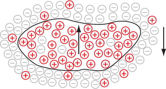
Figure 7.1: Inverted compact domain in a ferromagnetic system.

Let us consider a system with a predominantly ferromagnetic order, with most of the spins in the $(-)$ orientation. In this situation, we flip a compact domain of radius $R$ (see Figure 7.1).

The value of the exchange interaction energy in the bulk of this domain does not change with this reversal, but all the links across its boundary are inverted. Therefore, there is an increase $\Delta U\sim R^{D-1}$. As to the field-interaction energy the average value of $h_{\boldsymbol{x}}$ inside the domain is of course zero. On the other hand, the variance of the sum of $n$ Gaussian variables, each of variance $H$, is $\sqrt{n}H$. That is, we have $\Delta E_{\text{F}}=2E_{\text{F}}\sim HR^{D/2}$. Choosing a region with positive $E_{\text{F}}$, we then have

$$\Delta E=\Delta U+\Delta E_{\text{F}}=aR^{D-1}-bHR^{D/2},$$ (7.3)

where $a,b$ are positive constants. Therefore, if $D-1<D/2$ we see that these perturbations are actually energetically favourable, for large enough $R$. Hence, the ferromagnetic phase is unstable for $D<2$. The marginal case $D=2$ was considered in [binder:83] and also found to be unstable. Therefore, the lower critical dimension for the RFIM had to be $D_{\text{l}}\geq 2$ (other mechanisms than the domain-wall argument could destroy the long-range order in three or more dimensions). The issue was solved by the rigorous proof that $D_{\text{l}}=2$ [imbrie:84, bricmont:87, aizenman:89].

The disorder in the RFIM was thus showed to be strong enough to modify the phase diagram of the pure model profoundly, yet not so radical as to make the phase transition disappear altogether. The interest in the system was further enhanced when it was shown that it could be faithfully realised physically by a diluted antiferromagnet in a uniform field (DAFF) [fishman:79, cardy:84]. This ignited a considerable experimental effort (see [belanger:98] for a review).

In short, it was shown more than twenty years ago that the RFIM experiences a phase transition in three spatial dimensions and that the system is also of experimental interest through the DAFF. Despite a continuing analytical, experimental and numerical effort, however, almost all the details of this transition remain controversial.

In particular, characterising the phase transition proved to be no easy task from an analytical point of view (see [nattermann:97, dedominicis:06] for reviews of theoretical results). First of all, we have the general observation that the upper critical dimension for disordered systems is $D_{\text{u}}=6$ (as opposed to $D_{\text{u}}=4$ for pure models, cf. Chapter 2 and Section 7.2.1, below). Therefore, it is more difficult to predict the behaviour in the physically interesting case of $D=3$ from renormalisation-group expansions in $\epsilon=D_{\text{u}}-D$.

An example of the problems with perturbation expansions is afforded by the issue of dimensional reduction. In 1979, Parisi and Sourlas [parisi:79] presented an elegant supersymmetry argument by which the critical behaviour of the RFIM at dimension $D$ should be equivalent to that of the pure model in $D-2$. But this had to be wrong: we have already seen that there is a phase transition in $D=3$, while the Ising model has no ordered state in $D=1$. Parisi pointed out a possible flaw in the supersymmetric argument as soon as 1984 [parisi:84], but the issue has remained an active topic of research (see, e.g., [brezin:01, tissier:11] and references therein).

The experimental and numerical approaches to the problem are similarly plagued by severe intrinsic problems. The main one is perhaps posed by the peculiar critical behaviour of the DAFF/RFIM [villain:85, fisher:86b, nattermann:97]. In general, most authors work in the framework of an unconventional scaling theory, which we shall explain in Section 7.2.1, where the spatial dimension $D$ is replaced by $D-\theta$ in the traditional hyperscaling relation (2.19d). Here $\theta$ is a new critical exponent, believed to be $\theta\approx 1.5$ from theoretical arguments (cf. Section 7.2.1) but inaccessible to a direct computation both in experimental studies and in (canonical) Monte Carlo simulations.

The complete uncertainty in the determination of $\theta$ has allowed experimental and numerical works to report qualitatively different sets of values for the other critical exponents. One example of this is the experimental claim for a divergence in the specific heat [belanger:83, belanger:98], not observed numerically [hartmann:01]. We must note that the specific heat exponent is notoriously difficult to estimate numerically [malakis:06], especially considering that the expected divergence is very slow.

From the experimental point of view, an additional problem is posed by the uncertainty over the analytical form of the scattering line shape or structure factor. Different ansätze lead to mutually incompatible results for the thermal critical exponent, from $\nu=0.87(7)$ [slanic:99] to $\nu=1.20(5)$ [ye:04]. The first of these works also reported a value of $\eta=0.16(6)$ which, combined with a divergent specific heat ($\alpha\geq 0$), would violate hyperscaling if $\theta\approx 1.5$.

On the numerical front, the determination of $\nu$ has been at least as difficult, with estimates ranging from $\nu\approx 1$ to $\nu>2$ (see, e.g., [nattermann:97, wu:06, vink:10] for detailed lists). The most precise values have typically come from ground state studies. Hartmann and Nowak claimed $\nu=1.14(10)$ in [hartmann:99], although the value has recently been increased, with a recent estimate of $1.37(9)$ [middleton:02] (other recent works [malakis:06, fytas:11] give similar results). In general, these latest numerical estimates are outside the experimental range of values and only barely compatible with a divergent specific heat. Another recent work, [wu:06], gives $\nu=1.25(2)$ and $\alpha=-0.05(2)$. However, these values suffer from similar problems as experimental estimates (with which they are compatible) in that they do not satisfy hyperscaling bounds.

An additional source of uncertainty is the extremely low value of the magnetic critical exponent, believed to be $\beta\sim 0.01$. This exponent is also determined with almost no precision [nattermann:97, hartmann:99], the latest estimate of which we have notice being $\beta=0.007(5)$ [fytas:11]. The fact that $\beta$ is compatible with the first-order result of $\beta=0$ has led some authors to suggest the possibility that the phase transition in the DAFF may not be continuous. This claim is typically based on the finding of metastable signatures [sourlas:99, maiorano:07, wu:06] and casts doubts on the supposed universality between the DAFF and the RFIM.

A final issue is the lack of self-averaging in the DAFF, which has been extensively studied [parisi:02, malakis:06, fytas:11] and complicates any numerical analysis.

At the root of these problems is the deep physical issue of free-energy barriers, discussed in Chapter 3. Both experimentally and in canonical MC simulations, the system gets trapped in local minima, with escape times $\log\tau\sim\xi^{\theta}$, which makes it exceedingly hard to thermalise even relatively small systems and ensures that the statistics will be dominated by extremely rare events.

In the remainder of this chapter, after giving some definitions in Section 7.2, we shall examine more closely the reasons why canonical MC simulations of the DAFF fail.

7.2  Model and observables

We consider the diluted antiferromagnet in a field (DAFF), defined by the following Hamiltonian (as always $N=L^{D}$ Ising spins in a cubic lattice)

$$\mathcal{H} =\sum_{\langle\boldsymbol{x},\boldsymbol{y}\rangle}\epsilon_{\boldsymbol{x}}s_{\boldsymbol{x}}\epsilon_{\boldsymbol{y}}s_{\boldsymbol{y}}-h\sum_{\boldsymbol{x}}\epsilon_{\boldsymbol{x}}s_{\boldsymbol{x}}-h_{\text{s}}\sum_{\boldsymbol{x}}\epsilon_{\boldsymbol{x}}s_{\boldsymbol{x}}\pi_{\boldsymbol{x}}, \pi_{\boldsymbol{x}} =\mathrm{e}^{\mathrm{i}\uppi\sum_{\mu=1}^{D}x_{\mu}}$$ (7.4)

In addition to the Ising spins ($s_{\boldsymbol{x}}=\pm 1$), this Hamiltonian includes quenched occupation variables $\epsilon_{\boldsymbol{x}}$. These are equal to one with probability $p$ and equal to zero with probability $(1-p)$ and characterise the dilution of the system. The value of $p$ is not supposed to be important to the physics, so long as we keep our distance both from the percolation threshold of $p_{\text{c}}\approx 0.31$ [stauffer:84] and from the pure case. The $\epsilon_{\boldsymbol{x}}$ are quenched variables, which, recalling Section 2.2, means that we should perform first the thermal average for each choice of the $\{\epsilon_{\boldsymbol{x}}\}$ and only afterwards compute the disorder average. In the canonical ensemble we denote the thermal average by $\langle\cdots\rangle$ and the disorder average by $\overline{(\cdots)}$.

The Hamiltonian (7.4) includes a two-component applied field $(h,h_{\text{s}})$, coupled to the regular and staggered magnetisations

$$M =Nm=\sum_{\boldsymbol{x}}\epsilon_{\boldsymbol{x}}s_{\boldsymbol{x}},$$ (7.5)

$$M_{\text{s}} =Nm_{\mathrm{s}}=\sum_{\boldsymbol{x}}\epsilon_{\boldsymbol{x}}s_{\boldsymbol{x}}\pi_{\boldsymbol{x}},.$$ (7.6)

We shall continue to denote by $U$ the spin interaction component of the energy

$$U=Nu=\sum_{\langle\boldsymbol{x},\boldsymbol{y}\rangle}\epsilon_{\boldsymbol{x}}s_{\boldsymbol{x}}\epsilon_{\boldsymbol{y}}s_{\boldsymbol{y}}.$$ (7.7)

Therefore, the total energy $E$ of a given spin configuration can be written as

$$E=U-hM-h_{\text{s}}M_{\text{s}}.$$ (7.8)

In general, one is interested in the case $h_{\text{s}}=0$, but we will find this parameter useful later on.

In order to study spatial correlations we need to consider the staggered Fourier transform of the spin field

$$\phi({\boldsymbol{k}})=\sum_{\boldsymbol{x}}s_{\boldsymbol{x}}\pi_{\boldsymbol{x}}\ \mathrm{e}^{-\mathrm{i}{\boldsymbol{k}}\cdot{\boldsymbol{x}}}.$$ (7.9)

7.2.1 Phase transition in the DAFF: theoretical expectations

In this section, we give some heuristic arguments justifying the modified scaling relations expected for the DAFF, assuming a second-order scenario.

Let us consider the system at the paramagnetic-antiferromagnetic transition point $T_{\text{c}}(p,h)$ for a given dilution $p$ and field $h$. Now let us consider the effect of introducing a staggered magnetic field $h_{\text{s}}$. Unlike $h$, $h_{\text{s}}$ is coupled to the order parameter of the transition, so by definition (2.18) of the critical exponent $\delta$,

$$m_{\text{s}}\sim h_{\text{s}}^{1/\delta}.$$ (7.10)

Now, recalling that $m_{\text{s}}\sim xi^{-\beta/\nu}$, from (2.13) and (2.16) we have

$$h_{\text{s}}\sim\xi^{-\beta\delta/\nu}.$$ (7.11)

In addition, if we divide the system in the even and odd sublattices, the dilution implies that one is going to have $\sim L^{D/2}$ more spins than the other. This causes an excess staggered field $\delta h_{\text{s}}\sim\xi^{-D/2}$. Now, if we want the system to have a real transition as we approach the critical point $h_{\text{s}}\to 0$, we need

$$\frac{\delta h_{\text{s}}}{h_{\text{s}}}\xrightarrow{\ \ \xi\to\infty\ \ }0.$$ (7.12)

That is, we need

$$\frac{D}{2}\geq\frac{\beta\delta}{\nu}=\frac{2+\gamma-\alpha}{2\nu}\ ,$$ (7.13)

where we have used the scaling relation (2.19b).

If we plug the mean-field exponents into this equation, we obtain $D/2\geq 3$. Therefore, the upper critical dimension is in this case $D_{\text{u}}=6$.

Below $D_{\text{u}}$ we can in principle apply the hyperscaling law (2.19d). However, if we do this we obtain

$$\left.\begin{array}[]{rcl}\nu D&=&2-\alpha\\ \nu D&\geq&2+\gamma-\alpha\end{array}\right\}\quad\Longrightarrow\quad\gamma\leq 0.$$ (7.14)

Since the susceptibility critical exponent $\gamma$ must be positive, this is not possible.

The answer to this problem was given independently by Villain [villain:85] and by Fisher [fisher:86b]. We consider the system at the length scale of the correlation length. According to Widom scaling (see, e.g., [amit:05]), the free energy of this correlation volume $\xi^{D}$ is

$$F(\xi)\sim\xi^{D-(2-\alpha)/\nu}.$$ (7.15)

In conventional systems, the scale of variations of $F(\xi)$ is set by the thermal fluctuations, so $F(\xi)$ is of order one and the usual hyperscaling law $\nu D=2-\alpha$ follows. In our disordered system, however, the fluctuations due to the randomness dominate and

$$F(\xi)\sim\xi^{\theta},$$ (7.16)

where $\theta$ is a new, independent, critical exponent. Comparing (7.15) with (7.16) we read off the modified hyperscaling relation

$$2-\alpha=\nu(D-\theta).$$ (7.17)

In addition, from (7.13) we obtain the inequality

$$\theta\geq\gamma/\nu=2-\eta.$$ (7.18)

This last relation has been proven rigorously for a class of models [schwartz:85].

Some authors [aharony:76, schwartz:86] have suggested that the above inequality is saturated for the DAFF, giving

$$\theta=2-\eta,$$ (7.19)

so we would again have only two independent critical exponents.

Several heuristic arguments have been given to motivate Eq. (7.19) for the RFIM (see, e.g., [nattermann:97]), but we can also examine the issue directly in the DAFF.

Let us consider the system in the low-temperature phase with no field, so there is a non-zero spontaneous staggered magnetisation $m_{\text{s}}$ (in one of two orientations). As we said before, one of the sublattices (let us say the even one), has $\sim L^{D/2}$ more spins than the other. When the magnetic field $h$ is introduced, of the two orientations for the same $|m_{\text{s}}|$ the one where the even spins are aligned with the field will be more favourable.

Now, let us consider a region of radius $R$ where the odd sublattice is dominant (always possible to find, if the system is large enough). Clearly, inverting the magnetisation within this region aligns more spins with the field, lowering the total energy. The energy gain is $\sim-R^{D/2}m_{\text{s}}h$.

On the other hand, this inversion also has an energy cost, due to the surface energy. Therefore, the probability of inverting this region is going to be proportional to the exponential of

$$F(R)=R^{D/2}m_{\text{s}}-\varSigma R^{D-1},$$ (7.20)

where $\varSigma$ is the surface tension and we have neglected irrelevant constant factors in both terms. By definition of correlation length, this probability is maximum for $\xi=R$, where $F^{\prime}(R=\xi)=0$. Therefore,

$$F(\xi)\sim\xi^{D/2}m_{\text{s}}\sim\varSigma\xi^{D-1}.$$ (7.21)

Finally, by definition (7.16) of $\theta$ and using $m_{\text{s}}\sim\xi^{-\beta/\nu}$

$$\xi^{\theta}\sim\xi^{D/2}m_{\text{s}}\sim\xi^{D/2-\beta/\nu},$$ (7.22)

and we have

$$\theta=D/2-\beta/\nu,$$ (7.23)

which is equivalent to (7.19).

On the other hand, from $F(\xi)\sim\xi^{\theta}$ and (7.21), the surface tension is seen to scale as $\varSigma\sim\xi^{-(D-1-\theta)}$. Since we are assuming a second-order scenario, this has to vanish in the thermodynamical limit and we have

$$\theta<D-1,$$ (7.24)

(this last bound can be obtained without assuming the two-exponent scenario).

Finally, let us close this section by mentioning that the need for a third exponent is related to the existence of two correlation functions that scale differently,

$$S_{\text{c}}({\boldsymbol{k}}) =\overline{\braket{\phi({\boldsymbol{k}})\phi(-{\boldsymbol{k}})}}-\overline{\braket{\phi({\boldsymbol{k}})}}\ \overline{\braket{\phi(-{\boldsymbol{k}})}}\sim\frac{1}{k^{2-\eta}},$$ (7.25a)

$$S_{\text{d}}({\boldsymbol{k}}) =\overline{\braket{\phi({\boldsymbol{k}})}}\ \overline{\braket{\phi(-{\boldsymbol{k}})}}\sim\frac{1}{k^{4-\bar{\eta}}}.$$ (7.25b)

In this equation, $\phi({\boldsymbol{k}})$ is the staggered Fourier transform of the spin field, defined in (7.9), and $\bar{\eta}$ is

$$\bar{\eta}=2+\eta-\theta.$$ (7.26)

Notice that in the two-exponent scenario, $\bar{\eta}=2\eta$ and the disconnected propagator diverges as the square of the connected one

$$S_{\text{d}}\sim S_{\text{c}}^{2}.$$ (7.27)

7.3  The DAFF in canonical Monte Carlo simulations

In this section we carry out canonical Monte Carlo simulations of a DAFF system, to demonstrate the problems inherent in the traditional approach and motivate our tethered study of Chapter 8.

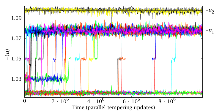
Figure 7.2: Time evolution of the interaction energy $u(t)$ —Eq. (7.7)— for the configuration at $T=1.6$, $\beta=2.4$ in $50$ different parallel tempering simulations of the same sample. We plot $50$ out of a total of $100$ runs. After a variable simulation time, most of the simulations fall into one of two metastable states, whose energies $u_{1}$ and $u_{2}$ we mark with straight black lines. In a thermalised situation, we would see tunnelling between the two states (or all of the runs reaching the same one, if only one is dominant).

In these simulations we have used parallel tempering, a common method to thermalise systems with free-energy barriers. The basic idea is running several copies of the same sample of the system concurrently, each at a different temperature. Every so often, we attempt to exchange copies at neighbouring temperatures. When the temperature is raised, the energy fluctuations increase and copies that would get trapped in metastable states can escape (see Appendix A for a full explanation of this method).

In our case, we have not attempted to conduct a full canonical study of the phase transition, we have just simulated a few samples. For each of them we performed many parallel tempering runs, using $40$ temperatures evenly spaced in the range $1.6\leq T\leq 2.575$ and choosing the field such that $\beta h=1.5$ (in this way, we intend to cross the phase diagram with a diagonal straight line). We considered a system size of $L=24$ and a dilution of $p=0.7$. These parameters are taken from [maiorano:07].

Figure 7.2 shows the time evolution of the interaction energy $u(t)$ for the lowest temperature ($T=1.6$, $h=2.4$) for $50$ runs of a single sample (we performed a total of $100$ such runs, but we only show $50$ to avoid cluttering the graph). We can see how, after a variable simulation length, most of the systems reach one of two metastable states, with interaction energies $u^{(1)}=-1.077\,35(8)$ and $u^{(2)}=-1.097\,3(7)$. The corresponding total energy densities, Eq. (7.8), are $e^{(1)}=-1.376\,08(2)$ and $e^{(2)}=-1.382\,0(2)$. The same qualitative picture is obtained for different samples.

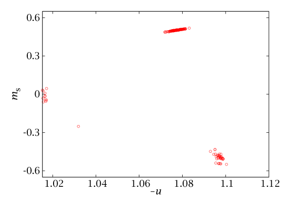
Figure 7.3: Scatter plot of the interaction energy $u$ and the staggered magnetisation for the $100$ runs of Figure 7.2. In each case we average the observables over the last $10\,000$ MCS, corresponding to the last $0.1\%$ of their whole Monte Carlo history. We see that the states with energies $u_{1}\approx-1.077$ and $u_{2}\approx-1.097$ correspond to systems in an antiferromagnetic phase (with opposite orientations).

The first conclusion we can draw from this plot is that parallel tempering has failed. Assuming $u_{1}$ and $u_{2}$ represent intermediate metastable states, not representative of the system’s equilibrium phase, we have failed to escape from them and reach the relevant regions of configuration space. On the other hand, assuming both are important to the equilibrium phase, then in a thermalised simulation we should see tunnelling between the two. Notice that obtaining the two estates in separate runs is not enough, we need to see the tunnelling in order to know their relative weights. However, we have not seen a single such jump, once the simulation reaches one of the two states it never escapes. In total we performed $100$ runs for this sample, each with $10^{7}$ parallel tempering updates, which suggests that the tunnelling probability is upper bounded by $10^{-9}$. In other words, parallel tempering is not able to thermalise the system in a reasonable amount of time. Notice that some of the simulations have not even reached one of the two metastable states

The second problem with the canonical approach is that of interpreting the results. Suppose we had considered runs many orders of magnitude longer than the ones plotted in Figure 7.2. Then, we would eventually begin to see the quick jumps from one state to the other, separated by long stays in each of them. This is the sort of metastable behaviour that one expects in the neighbourhood of a first-order phase transition, where two different phases have a similar weight, but are separated by large tunnelling barriers.

However, this interpretation would be wrong, as evinced by Figure 7.3. In it we represent a scatter plot of the staggered magnetisation against $u$ for the $100$ runs of Figure 7.2. It is readily apparent that the two states correspond to systems with opposite sign of the order parameter $m_{\text{s}}^{(1)}=0.502\,3(3)$, $m_{\text{s}}^{(2)}=-0.543(3)$. Therefore, the observed metastability would not correspond to jumps between an antiferromagnetic and a paramagnetic phase (the phase transition we want to study), but would rather reflect jumps between two antiferromagnetic states with different spin orientation.

This latter problem is intrinsic to the canonical description. Even if we could devise a more efficient thermalisation algorithm (or use a much faster computer) our results would still be contaminated by this spurious metastability and their statistical analysis dominated by extremely rare events.

CHAPTER VIII   The DAFF in the tethered formalism

We have just seen how traditional Monte Carlo methods are not well suited for the simulation of the DAFF. This was not only a case of thermalisation problems, but also revealed intrinsic limitations in the canonical approach, where the statistics is dominated by extremely rare events. In this Chapter we intend to demonstrate how a tethered approach can solve many of these difficulties.

8.1  The DAFF in the tethered ensemble

Our canonical investigation revealed that in the DAFF one has to deal with free-energy barriers separating states with different staggered magnetisations. Therefore, the appropriate reaction coordinate to tether is $m_{\text{s}}$. In addition, we are interested in a transition at non-zero magnetic field, where metastability could also appear. Therefore, we also tether the regular magnetisation $m$. Notice that by doing this, we do not need to specify the applied field for the tethered simulations. We simply simulate at zero field and then reweight the results as we did for the Ising model.

Let us consider the tethered description of a single sample. Recalling Section 4.1.1, we need a two-variable effective potential, whose gradient defines the tethered field, now a two-dimensional vector,

$$\boldsymbol{\nabla}\varOmega_{N}(\hat{m},\hat{m}_{\text{s}})=\biggl{(}\frac{\partial\varOmega_{N}(\hat{m},\hat{m}_{\text{s}})}{\partial\hat{m}},\ \frac{\partial\varOmega_{N}(\hat{m},\hat{m}_{\text{s}})}{\partial\hat{m}_{\text{s}}}\biggr{)}=\bigl{(}\langle\hat{b}\rangle_{\hat{m},\hat{m}_{\text{s}}},\ \langle\hat{b}_{\text{s}}\rangle_{\hat{m},\hat{m}_{\text{s}}}\bigr{)}$$ (8.1)

In this equation

$$\hat{b} =1-\frac{1/2-1/N}{\hat{m}-m},$$ (8.2a)

$$\hat{b}_{\text{s}} =1-\frac{1/2-1/N}{\hat{m}_{\text{s}}-m_{\text{s}}}.$$ (8.2b)

Then, the canonical averages in the presence of an external magnetic field with a regular component $h$ and a staggered component $h_{\text{s}}$ are related to the tethered expectation values through the Legendre transformation

$$\langle O\rangle(h,h_{\text{s}})=\frac{\int\mathrm{d}\hat{m}\int\mathrm{d}\hat{m}_{\text{s}}\ \langle O\rangle_{\hat{m},\hat{m}_{\text{s}}}\ \mathrm{e}^{-N[\varOmega_{N}(\hat{m},\hat{m}_{\text{s}})-\hat{m}\beta h-\hat{m}_{\text{s}}\beta h_{\text{s}}]}}{\int\mathrm{d}\hat{m}\int\mathrm{d}\hat{m}_{\text{s}}\ \mathrm{e}^{-N[\varOmega_{N}(\hat{m},\hat{m}_{\text{s}})-\hat{m}\beta h-\hat{m}_{\text{s}}\beta h_{\text{s}}]}},$$ (8.3)

although here we are interested in $h_{\text{s}}=0$, so we shall use the notation

$$\langle O\rangle(h)=\langle O\rangle(h,h_{\text{s}}=0).$$ (8.4)

And furthermore, we shall use the following shorthand

$$\varOmega_{N}^{(h)}(\hat{m},\hat{m}_{\text{s}})=\varOmega_{N}(\hat{m},\hat{m}_{\text{s}})-\beta h\hat{m},$$ (8.5)

and

$$\hat{\boldsymbol{B}}=\boldsymbol{\nabla}\varOmega^{(h)}_{N}(\hat{m},\hat{m}_{\text{s}})=\bigl{(}\braket{\hat{b}}_{\hat{m},\hat{m}_{\text{s}}}-\beta h,\ \braket{\hat{b}_{\text{s}}}_{\hat{m},\hat{m}_{\text{s}}}\bigr{)}.$$ (8.6)

According to the procedure described in Section 3.2, a tethered study of the DAFF would consist in a set of tethered simulations for fixed values of $(\hat{m},\hat{m}_{\text{s}})$ in a two-dimensional grid. From the value of the tethered field $(\braket{\hat{b}}_{\hat{m},\hat{m}_{\text{s}}},\braket{\hat{b}_{\text{s}}}_{\hat{m},\hat{m}_{\text{s}}})$ we would then reconstruct $\varOmega_{N}(\hat{m},\hat{m}_{\text{s}})$ and use (8.3).

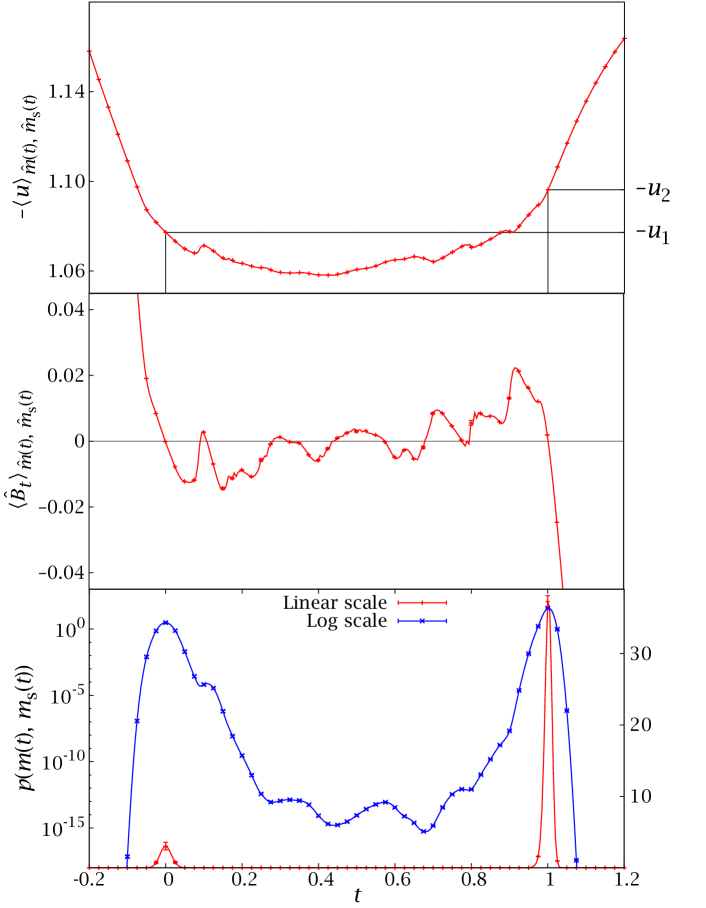
Figure 8.1: Result of a tethered investigation of the sample that we studied with canonical methods in Section 7.3. We join the two metastable states found in the canonical computation with a straight line and measure along this line the tethered expectation values for the energy $u$ and the projection of the tethered field $\hat{B}_{t}$ (top and middle, respectively). We simulated $281$ independent points along the line, but only plot one in five with error bar to avoid cluttering the graph. The tethered field has many zeros, defining saddle points in (8.3). Finally, the bottom panel shows the (exponential of the) integral of $\hat{B}_{t}$, defining the relative weight of the points along the path. Two peaks dominate, where the tethered values of the energy correspond to the two metastable states $u_{1}$ and $u_{2}$ that we found in Section 7.3. Notice the extremely low probability of the connecting region, which explains the difficulty to thermalise canonical simulations.

This is not, however, the most practical approach. For instance, it would involve the non-trivial numerical computation of a two-dimensional potential from its gradient, evaluated in a discrete grid. Instead, we note that, for a given $h$, only a very small region of the reaction coordinate space $(\hat{m},\hat{m}_{\text{s}})$ will have a relevant weight. In fact, the integral (8.3) is going to be dominated by the minima of the effective potential (recall our discussion of ensemble equivalence in Section 4.2). These will be given by the saddle-point equations

$$\boldsymbol{\nabla}\varOmega^{(h)}_{N}(\hat{m},\hat{m}_{\text{s}})=\hat{\boldsymbol{B}}=0,$$ (8.7)

that is

$$\begin{cases}\displaystyle\frac{\partial\varOmega_{N}}{\partial\hat{m}}&=\langle\hat{b}\rangle_{\hat{m},\hat{m}_{\mathrm{s}}}=\beta h,\\ \\ \displaystyle\frac{\partial\varOmega_{N}}{\partial\hat{m}_{\mathrm{s}}}&=\langle\hat{b}_{\mathrm{s}}\rangle_{\hat{m},\hat{m}_{\mathrm{s}}}=0.\end{cases}$$ (8.8)

In principle, some of these equations will correspond to local minima of $\varOmega^{(h)}_{N}$ and some to local maxima or to saddle points in the strict sense (a minimum in one direction, but a maximum in the other). In the case of local minima, the saddle points will correspond to metastable states, potentially relevant to the description of the equilibrium phase. Notice that we also obtained several metastable states in our canonical study of Section 7.3, but we were unable to know their relative weights. In the tethered approach, however, this is easily done by considering their potential difference, i.e., the line integral of $\hat{\boldsymbol{B}}$ along a connecting path.

Let us demonstrate this procedure for the sample of Section 7.3, where we had identified two metastable states (two local minima of $\varOmega^{(h)}_{N}$, in the tethered nomenclature). We first have to determine the values of $(\hat{m},\hat{m}_{\text{s}})$ that correspond to these saddle points using (8.8). This is easy, because our canonical study has given us the values of $m^{(i)}$ and $m_{\text{s}}^{(i)}$. We can now use (8.2a), setting $\hat{b}_{\text{s}}=0$ and $\hat{b}=\beta h=2.4$. Therefore, we know that $\hat{m}_{\text{s}}^{(i)}\simeq m_{\text{s}}^{(i)}+1/2$ and $\hat{m}^{(i)}\simeq m^{(i)}+1/(2(1-\beta h))$. From these starting guesses the actual saddle points are readily found. We can connect them with any path (because $\hat{\boldsymbol{B}}$ is a conservative field). Since the system is random, it is difficult to predict which will be the optimal connecting curve (in the sense of thermalisation), so we consider a simple straight line,

$$(\hat{m}(t),\hat{m}_{\text{s}}(t))=(\hat{m}^{(1)},\hat{m}_{\text{s}}^{(1)})(1-t)+(\hat{m}^{(2)},\hat{m}_{\text{s}}^{(2)}).$$ (8.9)

The whole computation is depicted in Figure 8.1. We performed tethered simulations for $281$ values of the parameter $t$ and measured the tethered expectation values of the energy $\braket{u}_{\hat{m}(t),\hat{m}_{\text{s}}(t)}$ and the tethered field $\hat{\boldsymbol{B}}$. These are plotted in the top and middle panels of the figure (for the tethered field we plot its projection $\hat{B}_{t}$ along the path).

Now, following (8.3), the probability density or relative weight of the points along the path is just

$$p(\hat{m}(t),\hat{m}_{\text{s}}(t))=\mathrm{e}^{-N\varOmega^{(h)}_{N}(\hat{m}(t),\hat{m}_{\text{s}}(t))},$$ (8.10)

where $\varOmega^{(h)}_{N}(t)$ is the line integral of $\hat{\boldsymbol{B}}$, with the integration constant chosen so that the whole weight is normalised. This probability density is plotted in the bottom panel of Figure 8.1, in both a linear and a logarithmic scale. We find that one of the two metastable has about ten times more weight than the other (curiously, fewer canonical simulations found the more relevant state). In addition, the two resulting peaks in the $p(\hat{m}(t),\hat{m}_{\text{s}}(t))$ are separated by a region with very low probability, explaining the difficulty of canonical simulations to tunnel between the two states. Interestingly enough, even within this low-probability sector we can see a rich structure of the $p(\hat{m}(t),\hat{m}_{\text{s}}(t))$ —equivalently, of the effective potential. In other words, we are seeing a quantitative example of a rugged free-energy landscape.

8.1.1 Self-averaging and the disorder average

In order to perform a quantitative analysis of the DAFF, we have to simulate a large number of samples and perform the disorder average. The naive way of doing this for a system with quenched disorder would be to measure $\hat{\boldsymbol{B}}$ and construct $\varOmega_{N}$ for each sample, then use Eq. (8.3) to compute all the physically relevant $\langle O\rangle(h)$. Only then would we average $\langle O\rangle(h)$ over the disorder.

This approach is, however, paved with pitfalls. First of all, computing a two-variable $\varOmega_{N}(\hat{m},\hat{m}_{\text{s}})$ from a two-dimensional $(\hat{m},\hat{m}_{\text{s}})$ grid is not an easy matter. In the previous section we avoided this problem by computing the saddle points first and then evaluating $\varOmega_{N}$ only along a path joining them. But this cannot be done efficiently and safely for a large number of samples. Even if it could be done, the free-energy landscape of each sample is very complicated, with many local minima, several of which could be relevant to the problem, so a very high resolution would be needed on the simulation grid.

Finally, even reliably and efficiently computing the canonical averages $\langle O\rangle(h)$ would not be the end of our problems. Indeed, as we discussed in Section 2.2.2, the canonical expectation values suffer from severe self-averaging violations. In this section we address all these problems and demonstrate the computational strategy followed in our study of the DAFF.

The first step is ascertaining whether the tethered averages themselves are self-averaging or not. We already know that, since we are going to be working with a large regular external field $h$, the relevant region for the regular magnetisation $m$ (and hence $\hat{m}$) is going to be exceedingly narrow (cf. Section 5.3, where the fields were much smaller). Therefore, we are going to explore the whole range of $\hat{m}_{\text{s}}$ for a fixed value of $\hat{m}=0.12$ (this smooth magnetisation is in the range where the saddle points typically lie for the applied fields we considered in Chapter 7).

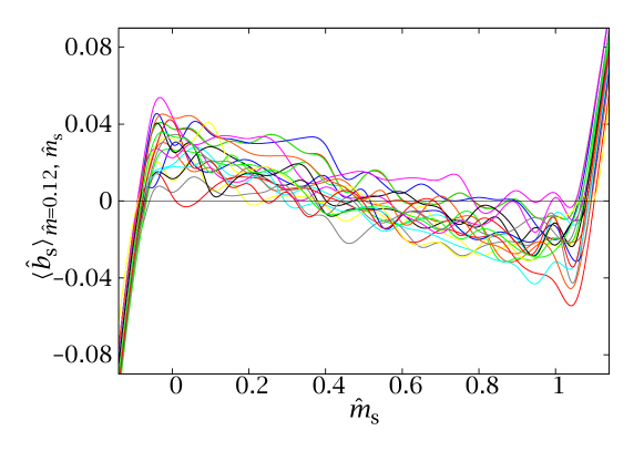
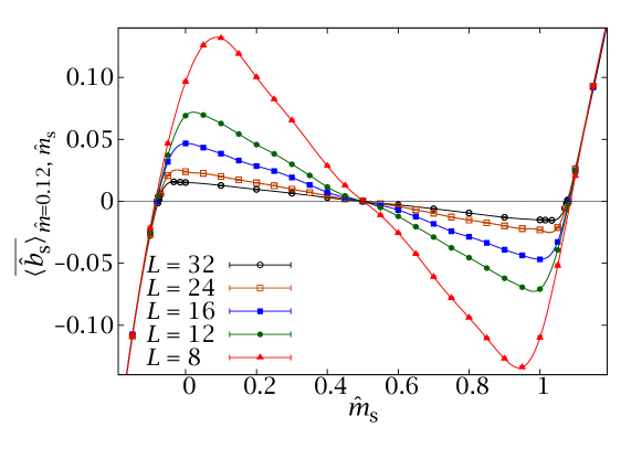
Figure 8.2: Top: Staggered component of the tethered magnetic field, $\langle\hat{b}\rangle_{\hat{m},\hat{m}_{\text{s}}}$ for $\hat{m}=0.12$ as a function of $\hat{m}_{\text{s}}$. We plot the results for several samples of an $L=24$ system at $\beta=0.625$. The curves are cubic splines interpolated from $33$ simulated points. We note that the errors are very small (invisible at this scale), so the fluctuations of the curves are not artifacts of the interpolation scheme. Bottom: Disorder-averaged $\overline{\langle\hat{b}_{\text{s}}\rangle}_{\hat{m},\hat{m}_{\text{s}}}$ for the same smooth magnetisation and temperature as the left panel, for all our system sizes. The plot shows the different behaviour of the regions inside the gap, where the staggered magnetic field goes to zero as $L$ increases, and outside it, where there is a non-zero enveloping curve.

We have plotted the staggered tethered magnetic field $\langle\hat{b}_{\text{s}}\rangle_{\hat{m}=0.12,\hat{m}_{\text{s}}}$ for $20$ samples of an $L=24$ system at $\beta=0.625$ in Figure 8.2—top. The different curves have a variable number of zeros, but all of them have at least three: one in the central region and two roughly symmetrical ones for large staggered magnetisation. The positions of the two outermost zeros clearly separate two differently behaved regions. Inside the gap the sample-to-sample fluctuations are chaotic, while outside it the sheaf of curves even seems to have an envelope. This impression is confirmed in the bottom panel of Figure 8.2, where we show the sample-averaged tethered magnetic field for several system sizes.

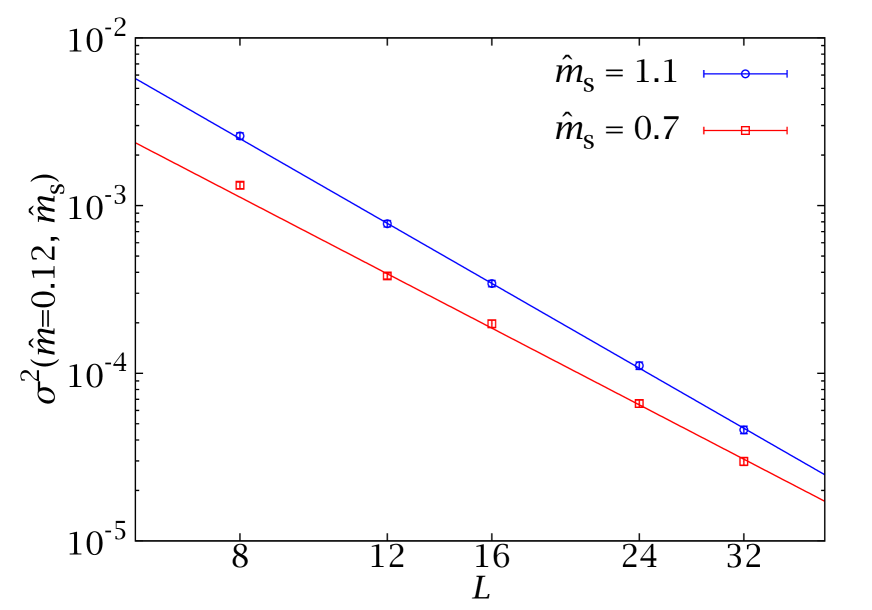
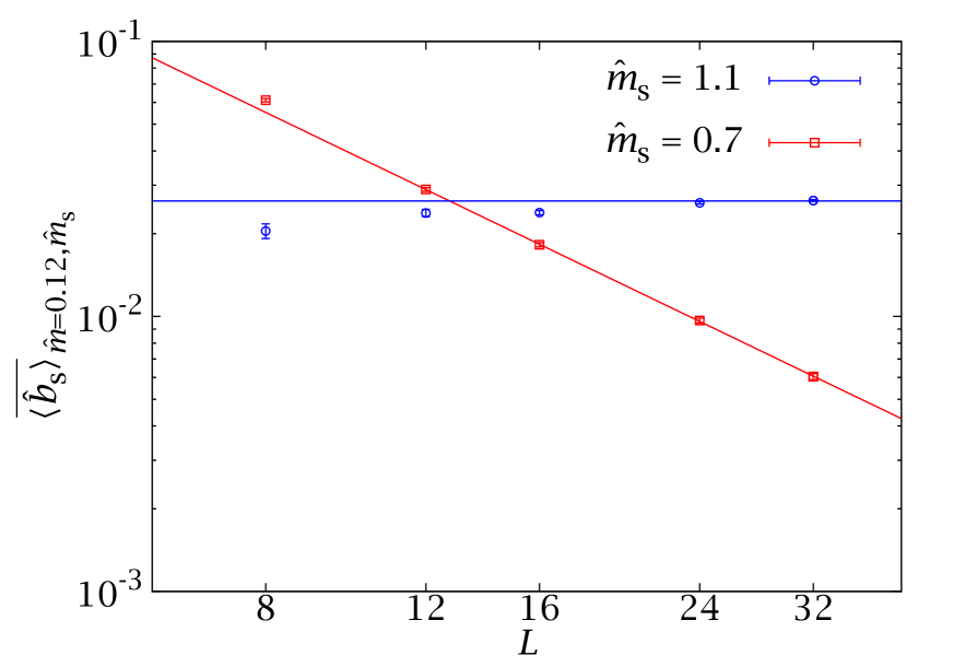
Figure 8.3: Left: Sample-to-sample fluctuations in the staggered component of the tethered magnetic field, Eq. (8.11), against system size. We show two sets of points, both at $\beta=0.625$ and $\hat{m}=0.12$, but for different values of $\hat{m}_{\text{s}}$. The red curve, corresponding to $\hat{m}_{\text{s}}=0.7$, is right inside the gap defined by the outermost zeros in Figure 8.2, while the blue curve ($\hat{m}_{\text{s}}=1.1$) is outside. Both are shown to decay with a power law. Right: Disorder average $\overline{\langle\hat{b}_{\text{s}}\rangle}_{\hat{m},\hat{m}_{\text{s}}}$ for the systems of the left panel. Inside the gap, the field goes to zero with $L$; outside it has a finite limit.

In order to quantify this observation we can study the fluctuations of the disorder-averaged $\overline{\langle\hat{b}_{\text{s}}\rangle}_{\hat{m},\hat{m}_{\text{s}}}$,

$$\sigma^{2}(\hat{m},\hat{m}_{\mathrm{s}}) = \overline{\left({\langle\hat{b}_{\mathrm{s}}\rangle}_{\hat{m},\hat{m}_{\mathrm{s}}}-\overline{\langle\hat{b}_{\mathrm{s}}\rangle}_{\hat{m},\hat{m}_{\mathrm{s}}}\right)^{2}}\ .$$ (8.11)

This quantity is plotted in the left panel of Figure 8.3. As we can see, it goes to zero as a power in $L$, so we also plot fits to

$$\sigma^{2}(\hat{m}=0.12,\hat{m}_{\text{s}})=A(\hat{m}_{\text{s}})L^{-c(\hat{m}_{\text{s}})}.$$ (8.12)

This would seem like a very good sign, because it could be indicative of self-averaging behaviour. However, it is not the whole story. If we recall the bottom panel of Figure 8.2, we see that inside the gap the tethered magnetic field itself, not only its fluctuations, goes to zero as $L$ increases. In fact, as shown in Figure 8.3, for $\hat{m}_{\text{s}}=0.7$, $\sigma^{2}\sim L^{-2.5}$, while $\overline{\langle\hat{b}_{\text{s}}\rangle}_{\hat{m},\hat{m}_{\text{s}}}\sim L^{-1.6}$. This means that the relative fluctuations $R_{\hat{b}_{\text{s}}}$, Eq. (2.41), do not decrease with increasing $L$. For the point outside the gap, however, the disorder average of the tethered magnetic field reaches a plateau. Furthermore, the fluctuations decay with $c=2.94(7)$, which is compatible with the behaviour $R_{\hat{b}_{\text{s}}}\sim L^{-D}$ of a strongly self-averaging system (in the language of Section 2.2.2).

In physical terms, this analysis means that the saddle point defined by a small, but non-zero, value of the applied staggered magnetic field $h_{\text{s}}$ would be self-averaging. We can now recall the well-known recipe for dealing with spontaneous symmetry breaking (see Section 5.4.1): consider a small applied field and take the thermodynamical limit before making the field go to zero. Translated to the DAFF, this means that we should solve the saddle-point equations (8.8) on average, rather than sample by sample, and then take the $h_{\text{s}}\to 0$ limit on the results,

$$\begin{cases}\displaystyle\frac{\partial\overline{\varOmega}_{N}}{\partial\hat{m}}&=\overline{\langle\hat{b}\rangle}_{\hat{m},\hat{m}_{\mathrm{s}}}=\beta h,\\ \\ \displaystyle\frac{\partial\overline{\varOmega}_{N}}{\partial\hat{m}_{\mathrm{s}}}&=\overline{\langle\hat{b}_{\mathrm{s}}\rangle}_{\hat{m},\hat{m}_{\mathrm{s}}}=0^{+}.\end{cases}$$ (8.13)

In other words, we are considering the disorder average of a thermodynamical potential, $\varOmega_{N}$, different from the free energy. This approach was first introduced in [fernandez:08], in a microcanonical context (the averaged potential was in that case the entropy).

In order to understand the limit $h_{\text{s}}\to 0^{+}$, it is convenient to keep in mind the analysis of the $p(\hat{m})$ for the Ising model in Sections 5.3 and 5.4.1. A small but positive $h_{\text{s}}$ exponentially suppresses the negative staggered magnetisation region and, as its value is decreased, it is equivalent to considering a ‘smeared’ saddle point and averaging over the whole sector with $\hat{m}_{\text{s}}>1/2$. A small but negative $h_{\text{s}}$ would have the corresponding effect in the $\hat{m}_{\text{s}}<1/2$ region. Since most of the interesting disorder-averaged observables are symmetric with respect to $\hat{m}_{\text{s}}=1/2$, we can gain statistics by averaging over the whole $\hat{m}_{\text{s}}$ range.

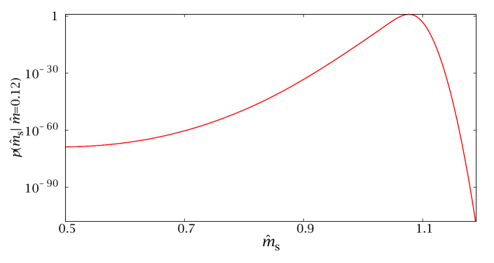
Figure 8.4: Disorder-averaged pdf of $\hat{m}_{\text{s}}$ conditioned to $\hat{m}=0.12$ for the system of Figure 8.2. Compare the simple structure of this graph with the bottom panel of Figure 8.1.

By doing this for fixed $\hat{m}=\hat{m}_{0}$ we obtain the probability distribution of $\hat{m}_{\text{s}}$, conditioned to $\hat{m}=\hat{m}_{0}$, which we will denote by $p(\hat{m}_{\text{s}}|\hat{m}_{0})$ (Figure 8.4). This probability density function can be used to average over $\hat{m}_{\text{s}}$ for fixed $\hat{m}$,

$$\overline{\langle O\rangle}_{\hat{m}}=\int\mathrm{d}\hat{m}_{\text{s}}\ p(\hat{m}_{\text{s}}|\hat{m})\overline{\langle O\rangle}_{\hat{m},\hat{m}_{\text{s}}}=\int\mathrm{d}\hat{m}_{\text{s}}\ \overline{\langle O\rangle}_{\hat{m},\hat{m}_{\text{s}}}\mathrm{e}^{-N\overline{\varOmega}_{N}(\hat{m}_{\text{s}}|\hat{m})},$$ (8.14)

where

$$\frac{\partial\overline{\varOmega}_{N}(\hat{m}_{\text{s}}|\hat{m})}{\partial\hat{m}_{\text{s}}}=\overline{\langle\hat{b}_{\text{s}}\rangle}_{\hat{m},\hat{m}_{\text{s}}}\ .$$ (8.15)

The zero in $\overline{\varOmega}_{N}(\hat{m}_{\text{s}}|\hat{m})$ is chosen so that $p(\hat{m}_{\text{s}}|\hat{m})$ is normalised (so $\overline{\varOmega}_{N}(\hat{m}_{\text{s}}|\hat{m})$ differs from the two-dimensional $\overline{\varOmega}_{N}(\hat{m},\hat{m}_{\text{s}})$ in a constant term). In practice, since the $p(\hat{m}_{\text{s}}|\hat{m})$ is not symmetric sample by sample, but only for the disorder average, considering the whole $\hat{m}_{\text{s}}$ range for ${\mathcal{N}}_{\text{samples}}$ disorder realisations is roughly equivalent to considering only the positive sector for $2{\mathcal{N}}_{\text{samples}}$.

With this process we have integrated out the dependence on $\hat{m}_{\text{s}}$. We now have a series of smooth functions $\overline{\langle O\rangle}_{\hat{m}}$, together with a smooth one-to-one function $h(\hat{m})=\overline{\langle\hat{b}\rangle}_{\hat{m}}/\beta$. Recalling our analysis of ensemble equivalence in Section 5.4.1, we see that $\overline{\braket{O}}_{\hat{m}(h)}$ and $\overline{\langle O\rangle}(h)$ are simply two quantities that tend to the same thermodynamical limit. Furthermore, for finite lattices the tethered definition $\overline{\braket{O}}_{\hat{m}}$ is better behaved statistically and arguably more faithful to the physics of an experimental sample. Therefore, we shall make the identification

$$\overline{\langle O\rangle}(h)=\overline{\braket{O}}_{\hat{m}},$$ (8.16)

exact in the thermodynamical limit, even for finite lattices.

8.2  Our tethered simulations

$L$	${\mathcal{N}}_{\mathrm{samples}}$	${\mathcal{N}}_{T}$	${\mathcal{N}}_{\hat{m}}$	${\mathcal{N}}_{\hat{m}_{\mathrm{s}}}$	${\mathcal{N}}_{\mathrm{MC}}^{\mathrm{min}}$	${\mathcal{N}}_{\mathrm{MC}}^{\mathrm{av}}$
8	1000	20	5	31	$7.7\times 10^{5}$	$7.7\times 10^{5}$
12	1000	20	5	35	$7.7\times 10^{5}$	$7.7\times 10^{5}$
16	1000	20	5	35	$7.7\times 10^{5}$	$7.7\times 10^{5}$
24	1000	40	5	33	$7.7\times 10^{5}$	$9.3\times 10^{5}$
32	700	40	4	25	$1.5\times 10^{6}$	$5.5\times 10^{6}$

Table 8.1: Parameters of our simulations. For each of the ${\mathcal{N}}_{\mathrm{samples}}$ disorder realisations for each $L$, we run ${\mathcal{N}}_{\hat{m}}\times{\mathcal{N}}_{\hat{m}_{\mathrm{s}}}$ tethered simulations with temperature parallel tempering. The ${\mathcal{N}}_{T}$ participating temperatures are evenly spaced in the interval $[1.6,2.575]$. For each size we report the minimum number of Monte Carlo steps (Metropolis sweep + parallel tempering). After the application of our thermalisation criteria, some of the simulations for $L\geq 24$ needed to be extended, leading to a higher average number of Monte Carlo steps (${\mathcal{N}}_{\mathrm{MC}}^{\mathrm{av}}$).

We can infer several useful conclusions from the analysis of the previous section

• The disorder average should be performed on the tethered observables, before computing the effective potential.

• It is best to analyse several values of $\hat{m}$ separately, since the average over $\hat{m}_{\text{s}}$ for each fixed $\hat{m}$ can be unambiguously related to the canonical average $\overline{\langle O\rangle}(h)$ via $h(\hat{m})=\overline{\langle\hat{b}\rangle}_{\hat{m}}/\beta$. In this way, we can study the phase transition that arises by varying the applied magnetic field at fixed $\beta$.

• For fixed $\hat{m}$ the conditioned probability $p(\hat{m}_{\text{s}}|\hat{m})$ has two narrow, symmetric peaks, separated by a region with extremely low probability.

Therefore, we have carried out the following steps

1. Select an appropriate grid of $\hat{m}$ values. This should be wide enough to include the critical point for the simulation temperature, and fine enough to detect the fluctuations of $\overline{\langle O\rangle}_{\hat{m}}$. These turn out to be very smooth functions of $\hat{m}$, so a few values of this parameter suffice, as we shall see.

2. For each value of $\hat{m}$, select an appropriate grid of $\hat{m}_{\text{s}}$. We start with evenly spaced points and after a first analysis add more values of $\hat{m}_{\text{s}}$ in the neighbourhood of the saddle points, as this is the more delicate and relevant region. In contrast with our study for the Ising model (Section C.2), the steepness of the peaks makes this second step crucial here, even for small lattices.

3. The simulations for each $(\hat{m},\hat{m}_{\text{s}})$ are carried out with the Metropolis update scheme of section 3.2.1. In addition, we use parallel tempering (cf. Appendix A). This is not needed in order to thermalise the system for $L<32$, but it is convenient since we also study the temperature dependence of some observables. Furthermore, the use of parallel-tempering provides a reliable thermalisation check (Section A.3.1). Section C.4 in Appendix C contains some information about our numerical implementation of TMC for the DAFF.

From Figure 8.4 we see that, if we only want to compute the $\langle O\rangle(h)$, the tethered simulations for $\hat{m}_{\text{s}}$ away from the peaks are worthless, since their contribution to the average over $\hat{m}_{\text{s}}$ is exponentially suppressed by a huge factor. We could have run tethered simulations only in a narrow range of $\hat{m}_{\text{s}}$ around the peaks, as we did in Section 5.4.1. As we shall see, however, some physically relevant quantities require that the whole range be explored, the most conspicuous being the hyperscaling violations exponent $\theta$.

The parameters of our simulations are presented in Table 8.1. The table lists the number ${\mathcal{N}}_{\hat{m}}$ of values in our $\hat{m}$ grid and the number of points in the $\hat{m}_{\mathrm{s}}$ grid for each, so the total number of tethered simulations for each sample is ${\mathcal{N}}_{\hat{m}}\times{\mathcal{N}}_{\hat{m}_{\mathrm{s}}}$.

The number of Monte Carlo steps in each tethered simulation is adapted to the autocorrelation time (see next section), the table lists the minimum length ${\mathcal{N}}_{\text{MC}}^{\text{min}}$ and the average length ${\mathcal{N}}_{\text{MC}}^{\text{av}}$ for each lattice size.

8.2.1 Thermalisation and metastability

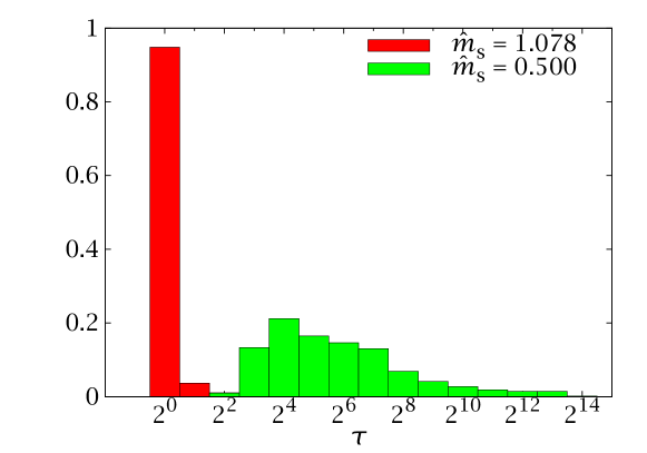
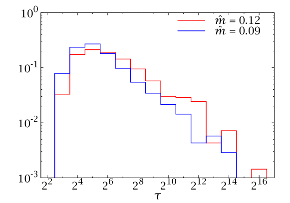
Figure 8.5: Histograms of thermalisation times for our $L=32$ simulations, at two values of $\hat{m}_{\mathrm{s}}$ for $\hat{m}=0.12$. Notice the logarithmic scale in the horizontal axis, which is in units of $300$ parallel-tempering steps. The saddle point (the peak in the probability distribution) at this $\hat{m}=0.12$ corresponds to $\hat{m}_{\mathrm{s}}=1.078$. Notice that we cannot measure times shorter than our measuring frequency of $300$ parallel-tempering steps, so the first bin should be taken as encompassing all shorter autocorrelation times. Only the samples with $\tau\gtrsim 2^{6}$ have to be extended from the minimum simulation time.

Figure 8.6: Same as Fig. 8.6, but now we consider several values of $\hat{m}$ for $\hat{m}_{\mathrm{s}}=0.8$ (in the hard thermalisation region far from the peak). The points for $\hat{m}=0.12$, closer to the critical point, exhibit a heavier long-time tail (mind the vertical logarithmic scale).

We have assessed the thermalisation of our simulations through the autocorrelation times of the system, computed from the analysis of the parallel tempering dynamics (see Section A.3.1). We require a simulation time longer than $100\tau_{\mathrm{int}}$. This process is only followed for $L\geq 24$. For smaller sizes we have simply made the minimum simulation time large enough to thermalise all samples.

The distribution of correlation times for our different samples turns out to be dependent on the value of $(\hat{m},\hat{m}_{\mathrm{s}})$. Considering first the variation of the average $\tau_{\mathrm{int}}$ with $\hat{m}_{\mathrm{s}}$ at fixed $\hat{m}$, we see that the peak of the $p(\hat{m}_{\text{s}}|\hat{m})$ and its adjoining region are much easier to thermalise (Figure 8.6). This region coincides with the only points that have a non-negligible probability density (Figure 8.4), i.e., the only points that contribute to the computation of the $\overline{\langle O\rangle}_{\hat{m}}$. This fact suggests a possible optimisation, that we will discuss in Section 8.7.

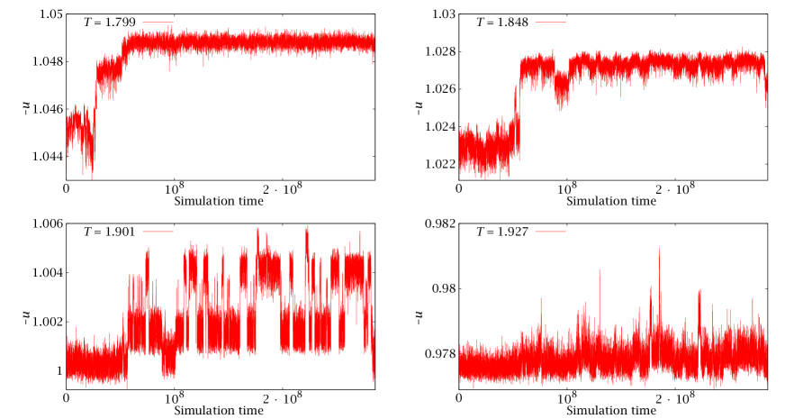
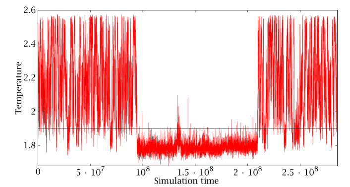
Figure 8.7: Time evolution (in number of parallel tempering steps) for the energy density $u$ for the same sample of an $L=32$ system at $\hat{m}=0.12$, $\hat{m}_{\text{s}}=0.7$ and different temperatures. For most temperatures the equilibrium value is quickly reached, but for a very narrow temperature range there are several competing metastable states (bottom-left panel for $T=1.901$).

Figure 8.8: Temperature random walk for one of the 40 replicated systems for the parallel tempering simulation of the sample in Figure 8.8. The flow is blocked at the same temperature that had several metastable states (marked with a horizontal line), see bottom-left panel in Fig. 8.8.

A second interesting result comes from studying the evolution of the $\tau_{\mathrm{i}nt}$ with $\hat{m}$. Figure 8.6 represents the histogram of autocorrelation times for $\hat{m}_{\mathrm{s}}=0.8$ (in the ‘hard’ region) for two values of $\hat{m}$. The distribution for $\hat{m}=0.12$ has a much heavier tail. As we shall see, this is due to the onset of a phase transition.

The difficulty in thermalising some samples stems from the coexistence of several metastable states, even for fixed $(\hat{m},\hat{m}_{\mathrm{s}})$. In Figure 8.8 we represent the time evolution of the energy $u$ for several temperatures of the same sample ($L=32$, $\hat{m}=0.12$, $\hat{m}_{\text{s}}=0.8$). As we can see, for a narrow temperature range several metastable states compete. This has a very damaging effect on the parallel tempering dynamics, whose flow is hindered whenever a configuration that is metastable for one temperature is very improbable in the next (see Figure 8.8).

For $L=32$, some points presented a metastability so severe that enforcing a simulation time longer than $100\tau_{\mathrm{int}}$ would require a simulation of more than $10^{9}$ parallel-tempering updates (one thousand times longer than our minimum simulation of $\sim 10^{6}$ steps). Thermalising these points (which constitute about $0.1\%$ of the total) would have thus required some $10^{6}$ extra CPU hours, with a wall-clock of many months. We considered this to be disproportionate to their physical relevance (they are all restricted to a region far from the peaks where the probability density is $<10^{-40}$, see Figure 8.4). Therefore, we have stopped these simulations at about $10\tau_{\mathrm{int}}$. This is still a more demanding thermalisation criterion than is usual for disordered systems and does not introduce any measurable bias in the physically relevant disorder-averaged observables. This can be checked in several ways:

• First of all, as we have already discussed, these points are restricted to a region in $\hat{m}_{\mathrm{s}}$ with probability density of at most $10^{-40}$. Therefore, even if there were a bias it would not have any effect in the computation of canonical averages.

• Even at the most difficult values of $(\hat{m},\hat{m}_{\mathrm{s}})$ the log₂-binning plot (the only thermalisation test typically used in disordered-systems simulations, see Section A.3) presents many logarithmic bins of stability (Figure 8.9, blue bars). Even if we subtract the result of the last bin from the others, taking into account statistical correlations (see Section A.3 and [fernandez:07]), several bins of stability remain (Figure 8.9, red bars). This is a very strict test, and one that even goes beyond physical relevance (because it reduces the errors dramatically from those given in the final results).

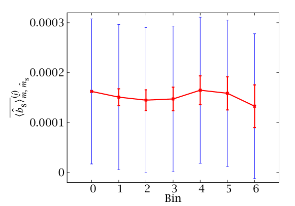
Figure 8.9: Time evolution of $\overline{\langle\hat{b}_{\mathrm{s}}\rangle}_{\hat{m},\hat{m}_{\mathrm{s}}}$ for $\hat{m}=0.12$, $\hat{m}_{\mathrm{s}}=0.5$, in a logarithmic scale (the first bin is the average over the second half of the simulation, the second bin the average over the second quarter and so on, cf. Section A.3). This is in the middle of the $(\hat{m},\hat{m}_{\mathrm{s}})$ region where thermalisation is hardest. The blue bars are the actual errors of our results and the red bars mark the error in the correlated difference of each bin with the first. Even for these reduced errors, we have several bins of convergence.

8.3  The effective potential

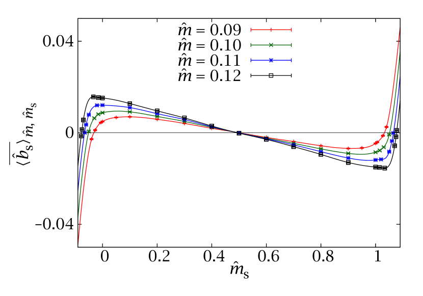
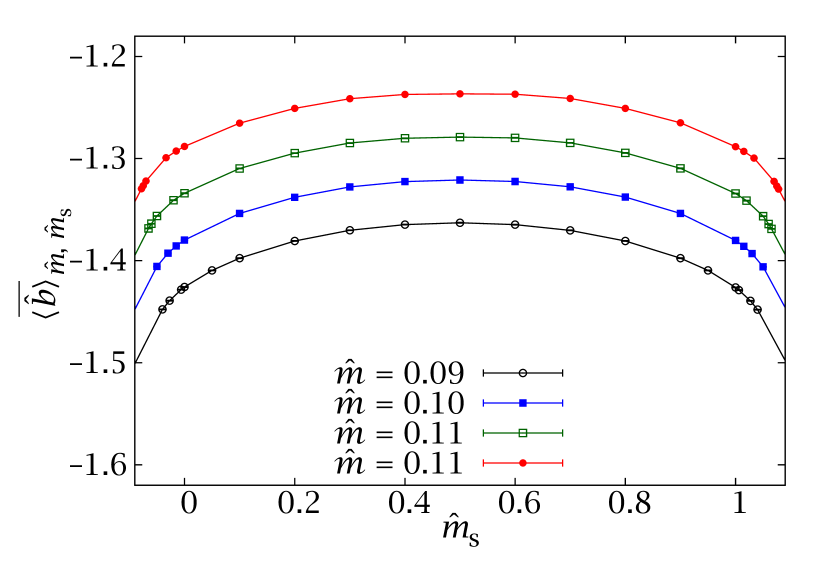
Figure 8.10: Left: Staggered component of the tethered field as a function of $\hat{m}_{\text{s}}$ for all the values of $\hat{m}$ in our $L=32$ simulations. Right: Same plot for the regular component of the tethered field.

As we discussed in detail in Section 8.1.1, we can learn much about the physics of the DAFF by studying the disorder-averaged saddle-point equations (8.13), which amounts to studying the disorder-averaged tethered field. To this end, we have plotted both components of the tethered field in Figure 8.10. Let us first consider the staggered component. In the region we are considering, the corresponding equation has three solutions for each $\hat{m}$: one in the paramagnetic region at $\hat{m}_{\text{s}}=0.5$ and two symmetric ones that get closer together as we lower $\hat{m}$. Notice that $\overline{\langle\hat{b}\rangle}_{\hat{m},\hat{m}_{\text{s}}}$ is negative, therefore when we lower $\hat{m}$ we are actually increasing $|m|$.

The other equation, $\overline{\langle\hat{b}\rangle}_{\hat{m},\hat{m}_{\text{s}}}=\beta h$, has two symmetrical solutions for each $\hat{m}$ (for values of $h$ in the range). The resulting structure of the effective potential is better understood with a two-dimensional plot of $\hat{\boldsymbol{B}}=\bigl{(}\overline{\langle\hat{b}\rangle}_{\hat{m},\hat{m}_{\text{s}}}-\beta h,\overline{\langle\hat{b}\rangle}_{\hat{m},\hat{m}_{\text{s}}}\bigr{)}$, which is the gradient of $\overline{\varOmega}_{N}^{(h)}(\hat{m},\hat{m}_{\text{s}})=\overline{\varOmega}_{N}(\hat{m},\hat{m}_{\text{s}})-\beta h\hat{m}$. We have plotted this vector in Figure 8.12, for $\beta h=-1.33$. There are three stationary points (circles in the figure):

• Two in the antiferromagnetic region, symmetric with respect to $\hat{m}_{\text{s}}$ and at the same $\hat{m}$. These are minima of the effective potential and, therefore, maxima of the probability density $p(\hat{m},\hat{m}_{\text{s}};h)$ (cf. Figure 8.12).

• One in the paramagnetic region, at $\hat{m}_{\text{s}}=0.5$ and at a different value of $\hat{m}$ from the other two. This is a saddle point, it is a maximum in the $\hat{m}_{\text{s}}$ direction and a minimum in the $\hat{m}$ direction (by symmetry considerations, these are its principal directions).

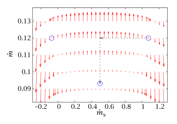
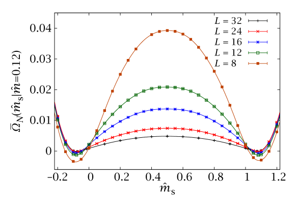
Figure 8.11: Plot of $\hat{\boldsymbol{B}}=\bigl{(}\overline{\braket{\hat{b}}}_{\hat{m},\hat{m}_{\text{s}}}-\beta h,\overline{\braket{\hat{b}_{\text{s}}}}_{\hat{m},\hat{m}_{\text{s}}}\bigr{)}=\boldsymbol{\nabla}\varOmega^{(h)}$ for $\beta h=-1.33$. There are three stationary points (circles): two symmetric antiferromagnetic minima at $\hat{m}\approx 0.12$ and a paramagnetic saddle point at $\hat{m}\approx 0.093$. The dashed arrow marks the integration path that we will use in Section 8.5.2.

Figure 8.12: Effective potential $\overline{\varOmega}_{N}(\hat{m}_{\text{s}}|\hat{m}=0.12)$, Eq. (8.15). The errors can hardly be seen at this scale (they are smaller than the width of the lines for the larger sizes).

We can use this analysis to make a first qualitative assessment of the order of the DAFF’s phase transition. Indeed, one of the most important features of a first-order transition is the emergence of metastability. The system, close to the transition point, has two metastable states, one ordered and the other disordered, characterised by peaks in the $p(\hat{m},\hat{m}_{\text{s}};h)$. As we modify the magnetic field, the relative weight of the peaks changes, until, at the transition point $p(\hat{m}^{\text{ordered}},\hat{m}_{\text{s}}^{\text{ordered}};h_{\text{c}})=p(\hat{m}^{\text{disordered}},\hat{m}_{\text{s}}^{\text{disordered}};h_{\text{c}})$. This is equivalent to the Maxwell construction in a microcanonical setting. However, in our analysis we have found no peak in the paramagnetic region, which would rule out the first-order scenario.

How, then, can we explain the metastable behaviour observed in previous work? Actually, our preliminary study of the DAFF in the canonical ensemble in Section 7.3 had the answer: the observed metastability is caused by the two coexisting antiferromagnetic peaks.

Let us consider $\overline{\varOmega}(\hat{m}_{\text{s}}|\hat{m})$ in Figure 8.12. In a canonical simulation the system would spend most of its time in one of the two antiferromagnetic minima, only very rarely tunnelling from one to the other. Notice that, even though the barrier $\Delta\overline{\varOmega}_{N}$ decreases with $L$, the escape time actually goes as $\exp[N\Delta\overline{\varOmega}_{N}]$, thus causing an exponential critical slowing down (cf. Figure 8.4, showing $\exp[N\Delta\overline{\varOmega}_{N}]\sim 10^{70}$ for an $L=32$ system). The precise behaviour of these free-energy barriers is of paramount importance to a characterisation of the physics and we shall dedicate Section 8.5.2 to its investigation.

8.4  Finite-size scaling study of the phase transition

The study of the effective potential in the previous section found no evidence of first-order behaviour in the DAFF, suggesting that its phase transition is continuous. Of course, promoting this statement to more than a working hypothesis would be premature, for several reasons. Not the least of which is that we have not yet shown that there actually is a phase transition in the studied $(\hat{m},\hat{m}_{\text{s}})$ region. In the remaining sections we shall both find this phase transition and characterise its properties. We shall first work at fixed $\beta=0.625$ and find the phase transition that appears when varying $h$ and we shall then examine the temperature behaviour at fixed $h$.

8.4.1 Scale invariance

One of the clearest signals of a continuous phase transition is the presence of scale invariance in the system. Therefore, our first step is computing the correlation length.

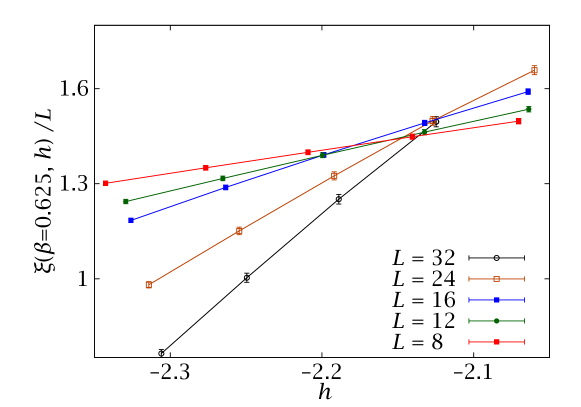
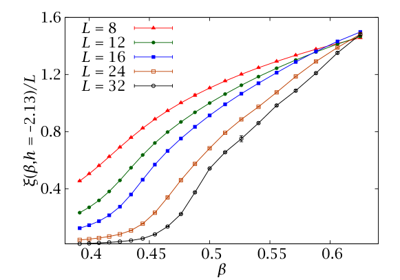
Figure 8.13: Correlation length in units of the system size as a function of the external magnetic field $h$, for $\beta=0.625$. The clear crossings at $h\approx-2.13$ signal a second-order phase transition.

Figure 8.14: Plot of $\xi/L$ as a function of the inverse temperature $\beta$ for $h=-2.13$. This is the approximate value of the critical field at $\beta=0.625$ (cf. Figure 8.14), which explains the convergence at the end of our temperature range.

Recalling definition (7.9) of the staggered Fourier transform we define the following propagator

$$F_{\hat{m}}({\boldsymbol{k}})=N\overline{\langle\phi({\boldsymbol{k}})\phi(-{\boldsymbol{k}})\rangle}_{\hat{m}},$$ (8.17)

which we use to define the second-moment correlation length (explained in Section 5.1)

$$\xi_{2}(h)=\frac{1}{2\sin(\uppi/L)}\left[\frac{F_{\hat{m}(h)}(0)}{F_{\hat{m}(h)}({\boldsymbol{k}}_{\mathrm{min}})}-1\right]^{1/2}.$$ (8.18)

Notice that we write $\xi_{2}(h)$ instead of $\xi_{2}(\hat{m})$, following our discussion of ensemble equivalence in Section 8.1.1.

The result of this computation is plotted in Figure 8.14. In it we can see a clear occurrence of scale invariance, signalling the onset of a second-order phase transition at $h\approx-2.13$. As a welcome bonus, the dependence of $\xi$ on $h$ is linear, which will simplify the analysis.

We can obtain a complementary picture by fixing the magnetic field and studying the temperature dependence. In Figure 8.14 we show this for $h=-2.13$. For each temperature and lattice, $\xi(h=-2.13)$ is obtained by linear interpolation in a plot analogous to Figure 8.14. This value of $h$ causes the critical temperature to appear at the very end of our simulated range. The reason for this choice is that the $\hat{m}_{\text{s}}$ grid for each $\hat{m}$ was optimised for $\beta=0.625$. As we move away from this temperature the peaks are only irregularly sampled, which causes larger statistical errors and potentially discretisation biases.

8.5  Computation of critical exponents

From the previous plots we can perform a Finite-Size Scaling [amit:05, zinn-justin:05] analysis in order to determine the critical exponents. As we discussed in Section 7.2.1, we need three independent critical exponents in order fully to characterise the phase transition of the DAFF, which we can choose as $\nu$, $\bar{\eta}$, $\theta$. In the following sections we shall compute these three exponents and then use additional observables to check the scaling and hyperscaling relations.

We shall apply the quotients method [ballesteros:96], which is based on Nightingale’s phenomenological renormalisation [nightingale:75]. Let us consider a system that experiences a second-order phase transition at a critical point $X_{\text{c}}$ (where the parameter $X$ is, in our case, either the applied magnetic field $h$ or the temperature). If some physical observable $O$ behaves as $(X-X_{\text{c}})^{-y_{o}}=x^{-y_{o}}$ near the transition point, then we expect the following dependence on a finite lattice (cf. Section 2.1.3), neglecting corrections to scaling,

$$O(L,x)=L^{y_{o}/\nu_{x}}f_{O}(xL^{1/\nu_{x}}).$$ (8.19)

In this formula $\nu_{x}$ is the exponent of the correlation length, $\xi\propto x^{-\nu_{x}}$ and $f_{O}$ is a smooth universal scaling function.

In order to define the quotients method, we write (8.19) in the following form

$$O(L,x)=L^{y_{o}/\nu_{x}}F_{O}(\xi(L,x)/L).$$ (8.20)

Now, for a pair of lattice sizes $L_{1}$ and $L_{2}=sL_{1}$ we identify the single value of $x$ such that $\xi(L_{1},x^{*})/L_{1}=\xi(L_{2},x^{*})/L_{2}$. At this point, we have

$$\frac{O(sL,x^{*})}{O(L,x^{*})}=s^{y_{o}/\nu_{x}}.$$ (8.21)

In Table 8.2 we have applied this method to several observables, using $s=2$,

$$\partial_{x}\xi \quad\longrightarrow\quad y_{o}=\nu_{x}+1,$$ (8.22)

$$M_{\mathrm{s}}^{2} \quad\longrightarrow\quad y_{o}=\bar{\gamma}=2\beta-3\nu_{x},$$ (8.23)

$$\partial_{x}M \quad\longrightarrow\quad y_{o}=\alpha.$$ (8.24)

In the following sections we shall analyse each critical exponent separately and compare the results with previous numerical and experimental work and with analytical conjectures.

$L$	$h^{*}(L)$	$\beta/\nu_{h}$	$\nu_{h}$	$\alpha/\nu_{h}$	$\nu_{\beta}$
8	$-2.178(4)$	0.0125(7)	0.887(5)	0.0765(25)	1.07[7](5)
12	$-2.140(5)$	0.0104(5)	0.790(9)	0.0781(27)	1.01[3](3)
16	$-2.123(3)$	0.0119(4)	0.742(7)	0.224(4)	1.10[13](7)

Table 8.2: Computation of the critical exponents with the quotients method, applied to pairs of lattices $(L,2L)$. The first four columns give results from the quotients at $h^{*}(L)$ for fixed $\beta=0.625$. The last column gives results for $\beta^{*}(L)$ at fixed $h=-2.13$. For this last value we give two error bars, distinguishing systematic and statistical errors.

8.5.1 Exponents $\nu$ and $\beta$

As a first application of the quotients method, we can compute the correlation length critical exponent, using equations (8.21) and (8.22). This exponent can be computed either from $\partial_{h}\xi$ (Figure 8.14) or from $\partial_{\beta}\xi$ (Figure 8.14).

In the first case, since the $h$ dependence is linear in all our simulated range, we simply fit $\xi(h)$ to a straight line and approximate $\partial_{h}\xi$ with its slope (as usual, we perform a different fit for each jackknife block) .

As to the temperature dependence, the analysis is more delicate for two reasons. The first is that $\xi(\beta)$ is no longer a straight line, the smaller sizes showing a clear curvature even very close to the intersection point. The second is that, as discussed above, the value of the correlation length for temperatures other than $\beta=0.625$ has some chaotic fluctuations due to discretisation error. Therefore, even if the data are correlated (as is the case for parallel tempering simulations), computing the temperature derivative is difficult.

Our solution has been to fit the high-$\beta$ region to a quadratic polynomial for $L\leq 16$ and to a straight line for $L\geq 24$. The aforementioned systematic effects cause the derivative to depend heavily on the fitting range. We have accounted for this effect in Table 8.2 by giving a second error bar, in square brackets.

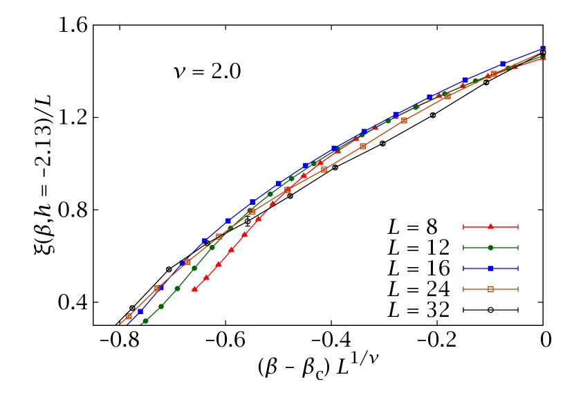
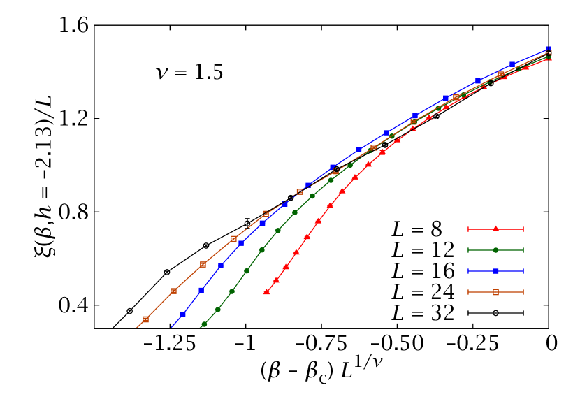
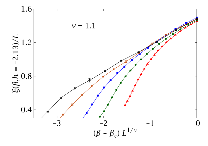
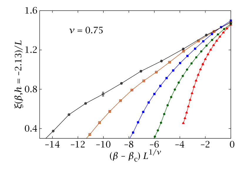
Figure 8.15: Scaling plots of $\xi/L$ for several values of the thermal critical exponent $\nu$. A very high value of $\nu$ causes a misleading collapse for low $L$, while our preferred values (bottom panels) are better at collapsing the larger sizes close to the intersection points.

Notice that exponents $\nu_{h}$ and $\nu_{\beta}$ should coincide, but we obtain $\nu_{h}\approx 0.75$ and $\nu_{\beta}\approx 1.05$. This discrepancy is mainly due to large corrections to scaling. In general, as discussed in the introduction to this chapter, attempts to determine $\nu$ have yielded values in a very broad range. We can see the reason in Figure 8.15, where we show scaling plots of $\xi(\beta)$ for values of $\nu$ in a very broad range. For each $\nu$ there is a temperature range that shows a seemingly good scaling. Therefore, attempting to estimate $\nu$ as the exponent that produces the best collapse, a method frequently employed for this and other models, is not only imprecise but also dangerous. By precisely locating the critical point and using the quotients method we minimise the effect of scaling corrections (but we do not eliminate them completely, as evinced by the incompatible values of $\nu_{h}$ and $\nu_{\beta}$).

Notwithstanding these difficulties, notice that our range of values for $\nu$ is in good agreement to that defined by the best experimental estimates: from $\nu=0.87(7)$ [slanic:99] to $\nu=1.20(5)$ [ye:04].

We can determine the critical exponent $\bar{\gamma}/\nu$ by applying the quotients method to $\overline{\langle M_{\text{s}}^{2}\rangle}(h)$. The results are quoted in Table 8.2. According to the scaling and hyperscaling relations (Section 7.2.1), $\bar{\gamma}/\nu=4-\bar{\eta}=3-2\beta/\nu$. Our resulting value of $\beta/\nu$ is very low, but different from zero. Recall that this exponent controls the evolution of the peaks in $p(\hat{m}_{\text{s}};h)$ (cf. Sections 5.2.2 and 6.4). In Figure 8.16 we can see that, indeed, the zero in $\overline{\langle\hat{b}_{\text{s}}\rangle}_{\hat{m},\hat{m}_{\text{s}}}$ shifts slowly but surely with increasing $L$. The figure is for fixed $\hat{m}=0.12\approx\hat{m}(h_{\text{c}})$.

The extremely small value of $\beta/\nu$ is one of the reasons for past claims of a first-order phase transition and is consistent with previous numerical studies.

8.5.2 The hyperscaling violations exponent $\theta$

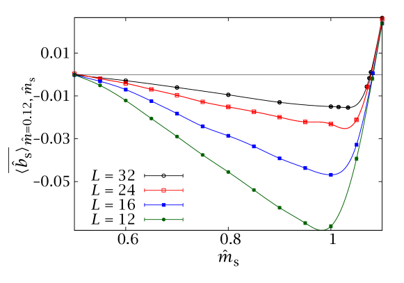
Figure 8.16: Plot of the staggered component of the tethered magnetic field, $\overline{\langle\hat{b}_{\mathrm{s}}\rangle}_{\hat{m},\hat{m}_{\mathrm{s}}}$ for $\hat{m}=0.12\approx\hat{m}(h_{\mathrm{c}})$ at $\beta=0.625$. This is a close-up of Figure 8.2—bottom, restricting the $\hat{m}$ range and eliminating the curve for $L=8$ in order better to see the $L$-evolution. The area under the curve between the two zeros gives the quantity $\Delta\overline{F}_{1}$, Eq. (8.29), which we can use to compute $\theta$. Notice the slow shift inwards of the antiferromagnetic zero, which marks the position of the peak in $p(\hat{m}_{\text{s}}|\hat{m})$.

The third and last independent critical exponent is $\theta$, which gives a measure of the violations to hyperscaling, Eq. (7.17). This exponent cannot be obtained from the canonical averages of physical observables at $h_{\text{c}}$, as we did for $\beta$ and $\nu$. Rather, its computation is an intrinsically tethered operation. Following Vink et al. [vink:10, fischer:11], we can relate $\theta$ to the free-energy barrier between the two coexisting states at the critical point,

$$\Delta\overline{F}_{N}\propto L^{\theta-D},$$ (8.25)

in this equation $\overline{F}_{N}$ is the free-energy density, as in equation (2.10). This is a specially interesting quantity to measure, since in a first-order transition $\theta\geq D-1$. Indeed, in a first order scenario the system would tunnel between the two pure phases (paramagnetic and antiferromagnetic) by building an interface. The free-energy barrier would then be associated to a surface tension. This in turn would be proportional to the dimension of the interface’s surface, which must be at least $D-1$.

We first notice that $\Delta\overline{F}_{N}$ is defined as the free-energy barrier between the two phases (disordered and antiferromagnetic) that form at the critical point $(\beta,h_{\mathrm{c}})$. Recalling our study of section 8.3 we see that this is equivalent to computing the $\Delta\overline{\varOmega}_{N}^{(h)}$ between the paramagnetic saddle point and one of the antiferromagnetic minima. We denote these two points by $(\hat{m}^{(1)},\hat{m}^{(1)}_{\mathrm{s}})$ and $(\hat{m}^{(2)},\hat{m}^{(2)}_{\mathrm{s}})$, respectively,

$$\Delta\overline{\varOmega}_{N}^{(h)}=\overline{\varOmega}_{N}^{(h)}(\hat{m}^{(1)},\hat{m}^{(1)}_{\mathrm{s}})-\overline{\varOmega}_{N}^{(h)}(\hat{m}^{(2)},\hat{m}^{(2)}_{\mathrm{s}}).$$ (8.26)

As always, this potential difference is simply the line integral of

$$\hat{\boldsymbol{B}}=\bigl{(}\overline{\langle\hat{b}\rangle}_{\hat{m},\hat{m}_{\text{s}}}-\beta h,\ \overline{\langle\hat{b}_{\text{s}}\rangle}_{\hat{m},\hat{m}_{\text{s}}}\bigr{)}$$ (8.27)

along any path connecting $(\hat{m}^{(1)},\hat{m}^{(1)}_{\mathrm{s}})$ and $(\hat{m}^{(2)},\hat{m}^{(2)}_{\mathrm{s}})$.

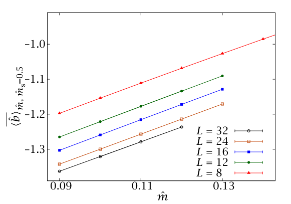
Figure 8.17: Tethered average $\overline{\langle\hat{b}\rangle}_{\hat{m},\hat{m}_{\text{s}}=0.5}$ for all our lattice sizes at $\beta=0.625$.

In our simulations we have not covered the $(\hat{m},\hat{m}_{\mathrm{s}})$ plane uniformly. Rather, we have simulated several slices with fixed $\hat{m}$. Therefore, the most convenient way to evaluate $\Delta\overline{\varOmega}_{N}^{(h)}$ is

1. At $\hat{m}=0.12\approx\hat{m}_{\text{c}}=\hat{m}(h_{\mathrm{c}})$, compute the potential difference between $(\hat{m}_{\text{c}},\hat{m}_{\text{s}}^{*})$ and $(\hat{m}_{\text{c}},0.5)$, where $\hat{m}_{\mathrm{s}}^{*}$ is the position of the peak of $p(\hat{m}_{\mathrm{s}}|\hat{m}_{\mathrm{c}})$ Notice that, since we are working at constant $\hat{m}$,

   $$\overline{\varOmega}_{N}^{(h)}(\hat{m}_{\text{c}},\hat{m}_{\text{s}}=0.5)-\overline{\varOmega}_{N}^{(h)}(\hat{m}_{\text{c}},\hat{m}_{\text{s}}^{*})=\overline{\varOmega}_{N}(0.5|\hat{m}_{\text{c}})-\overline{\varOmega}_{N}(\hat{m}_{\text{s}}^{*}|\hat{m}_{\text{c}}).$$ (8.28)

   This is just the integral

   $$\Delta F_{1}=\overline{\varOmega}_{N}(0.5|\hat{m}_{\mathrm{c}})-\overline{\varOmega}_{N}(\hat{m}_{\mathrm{s}}^{*}|\hat{m}_{\mathrm{c}})=\int\hat{\boldsymbol{B}}\cdot\mathrm{d}\boldsymbol{\ell}_{1}=\int^{0.5}_{\hat{m}_{\mathrm{s}}^{*}}\mathrm{d}\hat{m}_{\mathrm{s}}\ \overline{\langle\hat{b}_{\mathrm{s}}\rangle}_{\hat{m}_{\mathrm{c}},\hat{m}_{\mathrm{s}}}.$$ (8.29)

   In other words, $\Delta F_{1}$ is just the area under the curve in Figure 8.16. We can average $\Delta F_{1}$ for the symmetric path in the region with negative staggered magnetisation ($\hat{m}_{\text{s}}<1/2$).

2. The tethered average at $(\hat{m}_{\text{c}},\hat{m}_{\mathrm{s}}^{*})$ defines a value of $\beta h_{\mathrm{c}}$ through the saddle-point equation,

   $$\overline{\langle\hat{b}\rangle}_{\hat{m}_{\mathrm{c}},\hat{m}_{\mathrm{s}}^{*}}=\beta h_{\mathrm{c}}\,.$$ (8.30)

3. Consider the tethered values $\overline{\langle\hat{b}\rangle}_{\hat{m},\hat{m}_{\mathrm{s}}=0.5}$ as a function of $\hat{m}$ and interpolate the value $\hat{m}^{*}$ that satisfies

   $$\overline{\langle\hat{b}\rangle}_{\hat{m}^{*},\hat{m}_{\mathrm{s}}=0.5}=\beta h_{\mathrm{c}}\,.$$ (8.31)

   This turns out to be very easy to do because the $\overline{\langle\hat{b}\rangle}_{\hat{m},\hat{m}_{\mathrm{s}}=0.5}$ fall on a straight line (Figure 8.17).

4. Compute the potential difference between $(\hat{m}_{\mathrm{c}},\hat{m}_{\text{s}}\!=\!0.5)$ and $(\hat{m}^{*},\hat{m}_{\mathrm{s}}\!=\!0.5)$.

   $$\Delta F_{2}=\int\hat{\boldsymbol{B}}\cdot\mathrm{d}\boldsymbol{\ell}_{2}=\int^{\hat{m}^{*}}_{\hat{m}_{\mathrm{c}}}\mathrm{d}\hat{m}\ \bigl{(}\overline{\langle\hat{b}\rangle}_{\hat{m},\hat{m}_{\mathrm{s}}=0.5}-\beta h_{\text{c}}\bigr{)}.$$ (8.32)

5. The sum of $\Delta F_{1}$ and $\Delta F_{2}$ is equal to the integral of $\hat{\boldsymbol{B}}$ along a path joining the two saddle points $(\hat{m}^{(1)},\hat{m}_{\mathrm{s}}^{(1)})=(\hat{m}^{*},0.5)$ and $(\hat{m}^{(2)},\hat{m}_{\mathrm{s}}^{(2)})=(\hat{m}_{\mathrm{c}},\hat{m}_{\mathrm{s}}^{*})$. i.e., the free-energy barrier we were looking for,

   $$\Delta\overline{F}_{N}=\Delta F_{1}+\Delta F_{2}.$$ (8.33)

   This integration path is depicted with a dashed line in Figure 8.12. Notice that, in accordance with the study of Section 8.3, $\Delta F_{1}$ will be positive and $\Delta F_{2}$ negative.

We have implemented this procedure for all our lattices. Table 8.3 shows the resulting $\Delta\overline{F}_{N}$ and fits to

$$\Delta\overline{F}_{N}=AL^{3-\theta}.$$ (8.34)

$L$	$\Delta\overline{F}_{N}$	Fit range	$\theta$	$\chi^{2}/\mathrm{d.o.f.}$
8	0.033 82(29)	$L\geq 8\$	$1.448(9)$	5.56/3
12	0.017 56(15)	$L\geq 12$	$\mathbf{1.469}(13)$	$\mathbf{0.44\boldsymbol{/}2}$
16	0.011 38(9)	$L\geq 16$	$1.461\mathbf{\boldsymbol{(}20\boldsymbol{)}}$	0.16/1
24	0.006 08(5)
32	0.003 92(5)

Table 8.3: Computation of the hyperscaling violations exponent $\theta$ from the free-energy barriers $\Delta\overline{F}_{N}$. We report fits to (8.34), for different ranges. Our preferred final estimate is $\theta=1.469(20)$, taking the central value of the fit for $L\geq 12$ and the more conservative error of the fit for $L\geq 16$.

As our preferred final result we can give the central value of the fit for $L\geq 12$ with the error of the fit for $L\geq 16$. Therefore

$$\theta=1.469(20).$$ (8.35)

Notice that $\theta$ is close to the value $\theta=D/2$ that one would expect from a naive Imry-Ma argument [imry:75]. In particular, $\theta<D-1$, and therefore the metastable states do not define stable phases, which is yet another argument against a first-order transition.

Notice that the value of $\theta>0$ is also the reason for the exponential slowing down of this model. Indeed, we saw in Section 8.3 that the system gets trapped in local minima with escape times $\tau\sim\exp[N\Delta\overline{F}_{N}]\sim\exp[L^{\theta}]$ causing a thermally activated critical slowing down [fisher:86b, nattermann:97].

8.5.3 Scaling relations: the specific heat and $\alpha$

As discussed in the introduction to this chapter, there has long been disagreement as to whether the specific heat in the DAFF is divergent, as observed in experiments [belanger:83, belanger:98]. The specific heat critical exponent is generally difficult to obtain in numerical simulations and the self-averaging violations in the DAFF have not made things any easier [hartmann:01, wu:06, malakis:06],

Since we already have a complete set of independent critical exponents, we can obtain $\alpha$ from the hyperscaling relation (7.17). Using our range of values $0.75\leq\nu\leq 1.1$ and $\theta=1.469(20)$, we have the following bounds for $\alpha$,

$$0.32\leq\alpha\leq 0.85.$$ (8.36)

Clearly, the uncertainty in $\nu$ does not allow a good determination, yet we can safely exclude a non-divergent specific heat from our data ($\alpha<0$ would imply $\nu>1.3$). Furthermore, even the logarithmic divergence ($\alpha=0$) suggested by experimental work seems excluded. Notice, however, that the experimental values of $\nu$ together with hyperscaling relations, also imply $\alpha>0$. For instance, the result $\nu=0.87(7)$ of [slanic:99], taken with our $\theta=1.469(20)$, would give $\alpha\approx 0.67(10)$. Even the higher value $\nu=1.20(5)$ of [ye:04] would give $\alpha\approx 0.16(8)$.

We can attempt a direct determination of $\alpha$ from our simulations. We start by defining the specific heat as

$$C=\frac{\partial\overline{\langle m\rangle}}{\partial h}$$ (8.37)

In principle, at the critical field, $C\propto L^{\alpha/\nu}$, so we could compute $\alpha/\nu$ from $C$ using the quotients method. Unfortunately, the quotients method is ill-suited to this quantity, which features a large analytical background, so its scaling is more aptly described by $C\simeq A+B^{\alpha/\nu}$ [ballesteros:98b]. Therefore, one needs extremely large values of $L$ to reach the asymptotic regime where $C\sim L^{\alpha/\nu}$.

The behaviour of the quotients shown in Table 8.2 is consistent with the above expectation. Our results point to a divergent specific heat, but our estimates for the exponent $\alpha$ are clearly still very far from the asymptotic regime where (7.17) would be satisfied. An additional source of error is that our determination of the specific heat suffers from systematic effects due to the discretisation of $\hat{m}$. Indeed, while our $\hat{m}$ grid was more than adequate for a determination of $\partial_{\hat{m}}\xi$, which could be approximated by a straight line, the specific heat shows a clear curvature as a function of $\hat{m}$. We have interpolated it with a quadratic polynomial in order to estimate the derivative, but we would have needed more resolution in $\hat{m}$ to make a safe computation.

8.5.4 The two-exponent scenario and the experimental scattering line shape

We can close our FSS analysis of the phase transition by considering the two-exponent scenario discussed in Section 7.2.1. Recall that according to this proposal, $\theta=D/2-\beta/\nu$. From (8.35) and $\beta/\nu=0.011\,1(8)$ (combining the last two rows of Table 8.2) we have

$$\theta =1.469(20),$$ (8.38)

$$D/2-\beta/\nu =1.488\,9(8).$$ (8.39)

The two numbers are compatible.

We can use our results for the critical exponents to shed some light on the experimental situation. In an experimental study, the critical exponents are computed from fits to the scattering line shape or structure factor $S(k)$. We can write this quantity as

$$S(k)=S_{\text{d}}(k)+S_{\text{c}}(k),$$ (8.40)

where $S_{\text{d}}$ and $S_{\text{c}}$ are the connected and disconnected propagators defined in (7.25). Recall that these diverge as

$$S_{\text{d}}(k) \sim k^{-4+\bar{\eta}}+\ldots,$$ (8.41)

$$S_{\text{c}}(k) \sim k^{-2+\eta}+\ldots,$$ (8.42)

where the dots represent subdominant terms.

An experimental study of $S(k)$ faces, then, the considerable challenge of distinguishing two different divergences at $k=0$. One possibility is simply to disregard the difference and parameterise $S(k)$ with an effective anomalous dimension,

$$S(k)\sim k^{-2+\eta_{\text{eff}}}.$$ (8.43)

This procedure was employed in [ye:04], obtaining $\nu=1.20(5)$ and $\eta_{\text{eff}}=-0.51(5)$.

An alternative way, supported by our results, is to adopt the two-exponent ansatz (7.19), which can be rewritten as $2\eta=\bar{\eta}$. Then, the following approximation can be made:

$$S_{\text{d}}(k)=[S_{\text{c}}(k)]^{2}.$$ (8.44)

This avenue was followed in [slanic:99], yielding $\nu=0.87(7)$ and $\eta=0.16(6)$. This value of $\nu$ is right in the middle of our numerical bounds. However, taking into account (7.19), we would have

$$\theta=2-\eta=1.84(6),$$ (8.45)

which is clearly incompatible with our results.

The answer to this problem is that the approximation (8.44) is probably too naive. Even accepting that $\bar{\eta}=2\eta$, approximating all of $S_{\text{d}}$, and not just its most divergent term, as the square of $S_{\text{c}}$ is an excessive simplification. Clearly, a better theoretical parameterisation of $S(k)$ is needed. Our methods are well suited to a direct numerical approach to this question, left for future work.

8.6  Geometrical study of the critical configurations

The picture painted in the previous sections is that of a second-order transition; but one with quite extreme behaviour. Among its peculiarities we can cite an extremely small value of $\beta$ and large free-energy barriers, features both that are reminiscent of first-order behaviour. The free-energy barriers in the DAFF, however, diverge too slowly to be associated to the surface tension of well-defined, stable coexisting phases. But this only raises the question of what kind of configurations can give rise to such a behaviour.

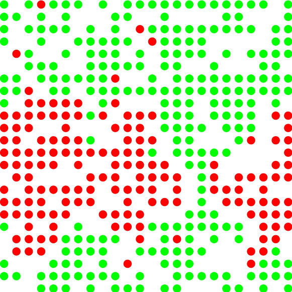
Figure 8.18: Equilibrium configuration for an $L=24$ system at $\beta=0.625$, $\hat{m}=0.12$, $\hat{m}_{\mathrm{s}}=0.5$.

In this section we study the geometrical properties of the minimal-cost spin configurations joining the two ordered phases at the critical point. To this end, we consider simulations at $\beta=0.625$, $\hat{m}=0.12\approx\hat{m}(h_{\mathrm{c}})$ and $\hat{m}_{\mathrm{s}}=0.5$. Recalling that $\hat{m}_{\mathrm{s}}\simeq m_{\mathrm{s}}+1/2$, this last condition expresses the fact that we are studying configurations with no global staggered magnetisation. This is a good example of an ‘inherently tethered’ study, that examines information hidden from a canonical treatment (cf. Figure 8.4, where we show that the region considered here has a canonical probability density of $\sim 10^{-70}$ for an $L=32$ system).

Figure 8.18 shows an example of such a configuration for an $L=24$ system. In order to make the different phases clearer, we are not representing the spin field $s_{\boldsymbol{x}}$, but the staggered field $s_{\boldsymbol{x}}\pi_{\boldsymbol{x}}$. As is readily seen, even if the global magnetisation is $m_{\mathrm{s}}\approx 0$, the system is divided into two phases with opposite (staggered) spin. In geometrical terms, most of the occupied nodes of the system belong to one of two large clusters with opposite sign. All the other clusters are orders of magnitude smaller, with most of the remaining spins forming single-site clusters.

At a first glance, this picture may seem consistent with a first-order scenario, where the system is divided into two strips whose surface tension gives rise to the free-energy barriers (see [martin-mayor:07] for an example of these geometrical transitions in a first-order setting). In order to test this possibility, we can study the evolution of the interface mass with the system size and compare it with the explicit computation of free-energy barriers done in Section 8.5.2.

$L$	${\mathcal{N}}_{\mathrm{samples}}$	${\mathcal{N}}_{\mathrm{interface}}$
12	3000	160.29(25)
16	3000	304.62(41)
24	3000	755.74(94)
32	700	1446.1(39)1

Table 8.4: Masses of the interfaces for our equilibrium configurations at $\beta=0.625$, $\hat{m}=0.12\approx\hat{m}_{\mathrm{c}}$, $\hat{m}_{\mathrm{s}}=0.5$. This mass grows as ${\mathcal{N}}_{\mathrm{interface}}\propto L^{c}$. From a fit, $c=2.240\,2(24)$, which is incompatible with our estimate of $\theta=1.469(20)$, confirming that the free-energy barriers are not associated to surface tensions.

Given a configuration, we first trace all the geometric antiferromagnetic clusters. We then identify the largest and second largest ones. Finally, we say that an occupied node belongs to the ‘interface’ if it belongs to the largest cluster and has at least one first neighbour belonging to the second largest one. We have computed in this way the interface ${\mathcal{N}}_{\mathrm{interface}}$ for our $700$ $L=32$ samples and for $3000$ samples for all our smaller systems (we have run additional simulations just at this point). Table 8.4 shows the result of this computation. A fit to

$${\mathcal{N}}_{\mathrm{interface}}=AL^{c},$$ (8.46)

for $L\geq 12$ gives $c=2.240\,2(24)$ with $\chi^{2}/$d.o.f. $=3.62/2$. If the metastability of the system were to be associated to a surface tension, then the free-energy barriers would have to scale with $c$. However, we saw in Section 8.5.2 that the actual scaling is $N\Delta\overline{F}_{N}\propto L^{\theta}$, with $\theta=1.469(20)$.

To understand the reason why this large interfaces are not responsible for metastable signatures, we have to look more closely at the geometry of the configurations. Indeed, we see in Figure 8.18 that there is a path connecting the spins in the green strip across the red one (there is only one green strip, since we are considering periodic boundary conditions).

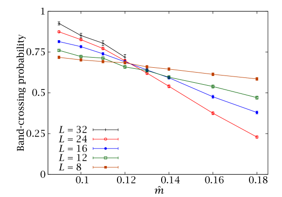
Figure 8.19: Probability of completing a path with constant staggered spin across the strip with opposite staggered magnetisation, see Fig. 8.18, for our spin configurations at $\beta=0.625$, $\hat{m}_{\mathrm{s}}=0.5$.

If we were to consider a complete tomography of this configuration, we would find several of these paths (which, of course, need not be contained in a plane). In other words, the phases are porous. This is in clear contrast to a first-order scenario in which the phases have essentially impenetrable walls. Now, this could be a peculiarity of the particular selected configuration. In order to make the analysis quantitative, we shall examine all of our samples and determine the strip-crossing probability $P$. This is defined as the probability of finding a complete path with constant staggered spin across the strip with opposite staggered magnetisation and we can compute it with the following algorithm:

1. For each configuration, compute the staggered Fourier transform (7.9) of the spin field at ${\boldsymbol{k}}_{\text{min}}^{(i)}$, for each of the three axes ($\phi_{x}$, $\phi_{y}$, $\phi_{z}$).

2. In a strip configuration, one of the $\phi$ will be much larger than the other two. Assume this is $\phi_{x}$, so the strips are perpendicular to the $OX$ axis.

3. Measure the staggered magnetisation $M_{\mathrm{s}}^{x}$ on each of the planes with constant $x$ and identify the plane $x=x_{\mathrm{max}}$ with largest $|M_{\mathrm{s}}^{x}|$. This plane will be at the core of one the strips.

4. Trace all the clusters that contain at least one spin on the $x=x_{\mathrm{max}}$ plane, but severing the links between planes $x=x_{\mathrm{max}}$ and $x=x_{\mathrm{max}}-1$.

5. If any of the clusters reaches the plane $x=x_{\mathrm{max}}-1$ there is at least a path through the strip with opposite magnetisation (the previous step has forced us to go the long way around, so we know we have crossed the strip).

We have plotted the strip-crossing probability $P(\hat{m})$ in Figure 8.19. Notice that $1-P$ behaves as an order parameter. If we keep increasing $\hat{m}$, so that we enter the ordered phase, the phases eventually become proper impenetrable strips, hence $P=0$ for large enough systems. On the other hand, for low $\hat{m}$, in the disordered phase, the strips become increasingly porous, so that $P=1$ in the limit of large systems. The crossover between these two regimes manifests in the crossing of the $P(\hat{m};L)$ at the phase transition point $\hat{m}\approx 0.12$.

8.7  Beyond $L=32$: optimising TMC simulations

The simulations listed in Table 8.1 required more than $700$ years of total CPU time and were carried out using a combination of large supercomputing facilities (Mare Nostrum of the Red Española de Supercomputación), large computing clusters (Terminus at BIFI) and grid resources (Piregrid). Even with the parallel scheme explained in Section C.4, the wall-clock for some of the toughest points has been of several months.

Essentially, by tethering the magnetisations we managed to remove the largest free-energy barriers of the systems. However, for large sizes, new barriers, associated to different reaction coordinates, began to appear. In order to eliminate these, one would have to tether additional quantities.

It may seem, then, that the methods described in this Chapter cannot be extended to larger lattices with current hardware. Actually, these simulations were intended to explore the physics of the DAFF thoroughly, perhaps sacrificing focus for breadth. In a more targeted study, however, we can take advantage of the model’s characteristics to optimise the simulations. In particular, we can highlight two interesting facts:

• Only a very narrow region around the saddle points has any significant weight for reconstructing canonical averages (Figure 8.4).

• It is much harder to equilibrate the region far from these peaks (Figure 8.6).

Combining these two observations, it turns out that, if our only interest is reconstructing canonical averages, we can achieve a qualitative reduction in simulation time by simulating only a narrow range around the peak in $p(\hat{m}_{\text{s}}|\hat{m})$ for each value of the smooth magnetisation $\hat{m}$. In fact, all the results discussed in this chapter, except for Sections 8.5.2 and 8.6, could have been computed in this simplified fashion.

We have demonstrated this optimisation by simulating $400$ samples of an $L=48$ system for $\hat{m}=0.12$. We use only ${\mathcal{N}}_{\hat{m}_{\text{s}}}=6$ (but we have to increase the number of temperatures in the parallel-tempering to $60$, in the same range, in order to keep the exchange acceptance high). Table 8.5 shows the value of $\hat{m}_{\text{s}}^{\text{peak}}$ as a function of $L$.

We can use the values of $\hat{m}_{\text{s}}^{\text{peak}}$ reported in Table 8.5 to attempt an alternative determination of $\beta/\nu$, following the method described in Section 5.2.2. In particular, we perform a fit to

$$|\hat{m}_{\mathrm{s}}^{\mathrm{peak}}-1/2|=AL^{-\beta/\nu}.$$ (8.47)

This is plotted in Figure 8.20. The result of the fit, with $\chi^{2}/$d.o.f. $=2.98/3$, is

$$\beta/\nu=0.011\,1(7).$$ (8.48)

This result is compatible with our computation with the quotients method in Table 8.2. Notice, however, that it does not take into account the uncertainty in $\hat{m}_{\mathrm{c}}$ (in Section 5.2.2 we worked at the exact $\beta_{\text{c}}$ and even in Section 6.4 we knew $\beta_{\text{c}}$ with many significant figures).

$L$	${\mathcal{N}}_{\text{samples}}$	$N_{\hat{m}_{\text{s}}}$	$\hat{m}_{\text{s}}^{\text{peak}}-1/2$
8	$1000\times 2$	31	0.585 85(87)
12	$1000\times 2$	35	0.582 39(54)
16	$1000\times 2$	35	0.581 54(36)
24	$1000\times 2$	33	0.578 39(24)
32	$700\times 2$	25	0.576 72(20)
48	400	6	0.574 91(33)

Table 8.5: Value of the peak position for our different system sizes. The result for $L=48$ is of comparable accuracy, despite being computed from only $6$ tethered simulations around the saddle point. Recall that for $L\leq 32$ we can average over the positive and negative peaks, so the number of samples for these systems is effectively double the value shown in Table 8.1.

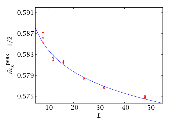
Figure 8.20: Position of the peak against $L$ from Table 8.5 with a fit to Eq. (8.47), giving $\beta/\nu=0.0111(7)$.

Part IV The Edwards-Anderson spin glass

CHAPTER IX   Spin glasses: an experimental challenge for theoretical physics

During the 20th century, the experimental study of magnetic alloys gradually led to the identification of a class of materials that suffered a ‘freezing transition’ at some critical temperature $T_{\text{c}}$. In particular, if we denote by $\boldsymbol{S}_{\boldsymbol{x}}$ the magnetic moment (spin) at site ${\boldsymbol{x}}$ in a lattice

• Below $T_{\text{c}}$, each of the spins freezes in some orientation, $\braket{\boldsymbol{S}_{\boldsymbol{x}}}_{t}\neq 0$.

• Though the freezing is collective, the spin orientations are random. In particular, the average orientation of the spins is zero: $\frac{1}{N}\sum_{\boldsymbol{x}}\braket{\boldsymbol{S}_{\boldsymbol{x}}}_{t}=0$. More generally, there is no long-range magnetic order of any kind

  $$\boldsymbol{M}_{\boldsymbol{k}}=\frac{1}{N}\sum_{\boldsymbol{x}}\mathrm{e}^{-\mathrm{i}{\boldsymbol{k}}\cdot\boldsymbol{r}}\braket{\boldsymbol{S}_{\boldsymbol{x}}}_{t}=0,\qquad\forall{\boldsymbol{k}}.$$ (9.1)

  Notice that this expression includes both the ferromagnetic order parameter, ${\boldsymbol{k}}=0$, and the antiferromagnetic one, ${\boldsymbol{k}}=(\uppi,\uppi,\uppi)$.

• The dynamical evolution takes place at macroscopic times below $T_{\text{c}}$.

The position of the freezing temperature is typically signalled by the appearance of a cusp in the imaginary part $\chi^{\prime\prime}(\omega)$ of the frequency-dependent magnetic susceptibility, although it has been proved that this freezing corresponds to an actual phase transition (cf. Section 9.1.3).

These systems were soon seen to have many interesting physical properties, which in turn generated a great deal of theoretical and experimental interest. In the early 1970s, the concept of ‘spin glass’ was introduced, and applied to random, mixed-interacting magnetic systems that experience a random, yet cooperative, freezing of spins below some critical temperature.

The random and mixed nature of the magnetic interactions gives rise to frustration (recall Figure 1.3) and this, in turn, generates a rugged free-energy landscape. Furthermore, the fact that spin glasses were particularly amenable to experimental investigation and theoretical modelling (see below) quickly established them as quintessential examples of complex systems.

In this chapter we shall begin by giving some brief notes on spin glasses from an experimental point of view in Section 9.1. This will also serve as an introduction to non-equilibrium physics and the concept of aging. We then discuss the generally accepted Edwards-Anderson model in Section 9.2, stating the main conclusions of the different (and incompatible) theoretical pictures that have been proposed for it. Finally, in Section 9.3 we motivate the numerical investigation of the problem that will be undertaken in Chapters 10 and 11.

9.1  The experimental spin glass

9.1.1 The canonical experimental spin glass: RKKY

As we said above, in order to have a spin glass system we need at least disorder and a mixture of ferromagnetic and antiferromagnetic interactions between the spins. In principle, we would be looking for a system whose spin Hamiltonian consisted of exchange interactions:

$$\mathcal{H}_{{\boldsymbol{x}}{\boldsymbol{y}}}=-J_{{\boldsymbol{x}}{\boldsymbol{y}}}\boldsymbol{S}_{\boldsymbol{x}}\cdot\boldsymbol{S}_{\boldsymbol{y}},$$ (9.2)

where we need to have both positive and negative $J_{{\boldsymbol{x}}{\boldsymbol{y}}}$.

The classical solution to these requirements is the Ruderman-Kittel-Kasuya-Yosida (RKKY) interaction [ruderman:54, kasuya:56, yosida:57]. We consider a noble metal with magnetic impurities (for instance, CuMn, for copper with manganese impurities). Then, the magnetic moments scatter the conducting electrons, which gives rise to an indirect exchange interaction: $\mathcal{H}_{{\boldsymbol{x}},{\boldsymbol{x}}+\boldsymbol{r}}=J(r)\boldsymbol{S}_{\boldsymbol{x}}\cdot\boldsymbol{S}_{{\boldsymbol{x}}+\boldsymbol{r}}$. For a large separation between impurities, we can write the coupling strength as

$$J(r)\simeq J_{0}\frac{\cos(2k_{\text{F}}r+\phi)}{(k_{\text{F}}r)^{3}},$$ (9.3)

($k_{\text{F}}$ is the Fermi momentum of the metal). Since the positions of the impurities or, in other words, the distances between the spins, are random, the oscillating nature of $J(r)$ will generate precisely the random mixture of ferromagnetic and antiferromagnetic couplings that we need.

9.1.2 Aging and other non-equilibrium phenomena

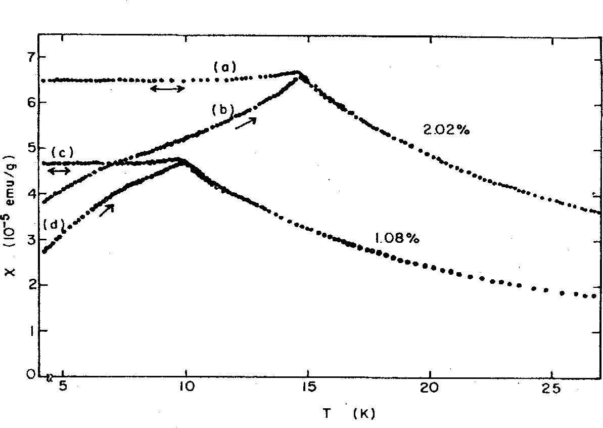
Figure 9.1: Comparison of the zero-field-cooled ($b$ and $d$ curves) and field-cooled susceptibilities ($a$ and $c$) for two samples of CuMn with different concentration of impurities. Graph from [nagata:79], as quoted in [binder:86].

The physical properties observed in spin-glass simulations are rich and surprising (see [binder:86, mydosh:93] for reviews). The main feature is that, in general, the relaxation times below $T_{\text{c}}$ are not only macroscopic, but large enough for the system to be out of equilibrium for the whole of the experiment. When the spin glass evolves at fixed $T_{1}<T_{\text{c}}$, some frozen or spin-glass phase slowly forms. In this situation, the system is said to age [vincent:97]: the response to a field variation depends on the time spent at $T_{1}$.

Let us see some examples of this. First we consider the experiment quoted in Figure 9.1. In it, the authors measured the magnetisation $M$ induced in a spin glass by a small applied field $h$ and used it to define a dc susceptibility $\chi_{\text{dc}}=M/H$. They then consider two experimental protocols. In the first one (field-cooling) they apply the field above $T_{\text{c}}$ and cool the system down to $T_{1}<T_{\text{c}}$, without switching off the field. The resulting curve is reversible if the temperature variation is cycled and it has the peculiarity that the $\chi_{\text{dc}}^{\text{FC}}$ becomes constant below $T_{\text{c}}$. In the second (zero-field cooling) the temperature is lowered to $T_{1}<T_{\text{c}}$ without applying any field. Then, the field is activated and the sample is reheated across the critical temperature. Above $T_{\text{c}}$, $\chi_{\text{dc}}^{\text{ZFC}}$ coincides with the field-cooled version, but this is not the case in the frozen phase. There, the curve is no longer constant, but increasing with $T$. Furthermore, while the FC curve was reversible, this one is not and it also depends on the temperature-variation rate. We are seeing a system out of equilibrium. In fact, if, after zero-field-cooling the system, we were to switch on the field and let the system evolve at fixed temperature, the susceptibility would grow slowly, approaching the FC value but never reaching it, even for waiting times of several hours.

A different, but related, example is the thermoremanent magnetisation. In this case, one cools the system in a field down to $T_{1}<T_{\text{c}}$, then waits for a time $t_{\text{w}}$, switches off the field and measures the decay of the remanent magnetisation when a time $t$ has passed after switching off the field. It turns out that this magnetisation depends both on $t$ and on the waiting time $t_{\mathrm{w}}$ that the system evolved in a field (the decay is slower for longer $t_{\mathrm{w}}$). This phenomenon is called aging. For a rapid cooling, the remanent decays as a function of $[(t+t_{\mathrm{w}})/t_{\mathrm{w}}^{\mu}]$ [rodriguez:03], so $t_{\mathrm{w}}$ is the only recognisable time scale. If $\mu=1$ we say that we have full aging.

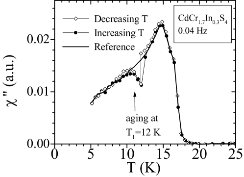
Figure 9.2: Memory and rejuvenation effects in an experimental spin-glass (see text for explanation). Figure taken from [jonason:98].

Notice that the concept of aging also applies to the coarsening dynamics of ferromagnetic systems, although there the process is much faster [sicilia:08]. However, let us stress that the differences between the dynamics of spin glasses and ferromagnets are much more profound than a simple change of speed. As an example of this, let us consider the experiment in Figure 9.2, taken from [jonason:98]. In this study, the authors took an experimental sample and measured the imaginary part $\chi^{\prime\prime}$ of the ac susceptibility as the temperature was varied. The applied field had a low frequency of $\omega/2\uppi=0.04$ Hz. In particular, they took the following three steps:

1. Starting at some temperature above $T_{\text{c}}$, they cool the system at a constant slow rate of $0.1$ K/min and then reheat it at the same rate. This cooling rate (in terms of the logarithmic derivative of the temperature), is very small compared with the frequency, $\omega$, which is equivalent to considering a regime where $t\ll t_{\mathrm{w}}$. The resulting $\chi^{\prime\prime}(T)$ is seen to be essentially reversible and represented by a thick black line. Notice the cusp at the transition temperature $T_{\text{c}}\approx 15$ K.

2. Back at the maximum temperature, the system is cooled again at the same rate (curve with empty diamonds). Now, however, they stop the cooling at $T_{1}<T_{\text{c}}$ and let the system age for a few hours. This produces a ‘dip’ in the $\chi^{\prime\prime}$ curve.

3. They resume the cooling and the susceptibility quickly returns to the reference curve, as if it had not aged at all. This effect is often named rejuvenation.

4. Now, the system is reheated at the same rate, without stopping at $T_{1}$ (curve with black diamonds). Surprisingly, the aging dip in the susceptibility is reproduced. Therefore, the rejuvenation of the previous step was not complete: the system has retained some memory of its previous aging.

No longer can we talk of a simple, temperature-independent spin-glass phase as in a ferromagnet. A picture of thermally activated barriers is also discarded, since the time spent at $T_{1}$ does not contribute to aging at $T_{2}<T_{1}$. Instead, we have some sort of temperature chaos: the appropriate spin-glass phase at $T_{1}$ looks completely random from the point of view of the system at $T_{2}$.

Still, even if the dynamical behaviour of spin glasses is very complex, there is some regularity. We shall see in Section 9.2.4 how it is possible to make experimentally testable predictions for several non-equilibrium quantities.

9.1.3 Spin glasses as models for general glassy behaviour

Structural glasses are formed when the viscosity of a liquid grows so much that the latter loses its ability to flow. The system drops out of equilibrium and its microscopic structure seems frozen. However, there is no long-range order: a still photo of the molecular arrangement would show no great difference from that of a dense liquid.

The above picture is, in qualitative terms, much the same as the one we painted at the beginning of this chapter, when introducing the spin-glass transition. This is so despite the fact that the physical causes for the two kinds of freezing processes are very different.

This observation is, of course, the motivation for the name of ‘spin glasses’ but, more than that, it is also the reason for much of their physical relevance. Indeed, taking spin glasses as model systems for investigating general glassy behaviour has many advantages, both from an experimental and from a theoretical point of view

• The nature of glass formation is still poorly understood, it has not yet been possible to relate it to a reproducible thermodynamical phase transition. On the other hand, the freezing of magnetic moments in spin glasses is known to be a phase transition, both in experiments [gunnarsson:91], where one observes a diverging non-linear susceptibility, and in theoretical models [palassini:99, ballesteros:00]. Knowing that one is really below a proper critical temperature has many advantages from the point of view of analysis and interpretation of results.

• In both classes of systems, the experimental determination of characteristic length scales is very difficult (the microscopic correlations are not accessible and one has to use an indirect determination via some susceptibility). However, spin-glass systems have two advantages: (i) The size $\xi$ of the glassy domains is much larger in spin glasses, and therefore easier to access experimentally (compare, e.g., [joh:99, bert:04] with [berthier:05]). (ii) In experiments on structural glasses, the measurements are specially delicate and taken with a variety of methods (in [berthier:05] they estimate the enthalpy fluctuations from measurements of the dielectric susceptibility). Spin-glass experiments, on the other hand, use SQUIDs, allowing for a far greater precision and convenience.

• The free-energy barriers in fragile glasses grow with a power law, while in spin glasses this growth is $\sim\log\xi$, as we shall see.

• Finally, spin glasses are easier to model theoretically (lattice models with simple interactions), making their subsequent analytical and numerical investigation more straightforward (although by no means easy, as we shall see in Section 9.2).

Still, even if we accept that spin glasses are more convenient model systems and that they have a qualitatively similar behaviour to structural glasses, we need some concrete, quantitative bridge between both systems, if only to see how far we can take the analogy.

In this sense, the study of dynamical heterogeneities can provide a valuable common ground. This topic has received much experimental attention in the last two decades [ediger:00, weeks:00, kegel:00, vidal-russell:00, oukris:10, berthier:11] and, has, in fact, been identified as the key to understanding the statistical mechanics of amorphous solids. Indeed, even though in structural glasses there is no long-range order, there are non-trivial spatiotemporal fluctuations, caused by the wide distribution of relaxation rates across the system. A thorough understanding of these dynamical heterogeneities can therefore give many clues on the nature of the glassy phase.

This heterogenous dynamic behaviour has recently been studied numerically in spin-glass systems [castillo:02, castillo:03, jaubert:07, aron:08]. In this context, the dynamical heterogeneities can be characterised by a two-time correlation length $\zeta(t,t_{\mathrm{w}})$, although the time scales that have been traditionally reachable in simulations have not permitted the authors to see correlation lengths greater than a couple of lattice spacings. At the same time, some recent experimental works suggest [oukris:10] that $\zeta$ will soon be accessible experimentally. Therefore, there is every indication that work on dynamical heterogeneities in structural and spin glass systems is soon going to converge in a unified approach. In the following chapters we shall dedicate much attention to $\zeta$, which will be the basis of a finite-time scaling paradigm for the study of non-equilibrium dynamics.

9.2  The theoretical spin glass: the Edwards-Anderson model

The complexity of the experimental spin-glass phase is both an incentive and a formidable challenge for theoretical physics. We need a system simple enough to allow for, at least, some level of analytical treatment yet complex enough to explain the rich physics observed in experiments.

The first obstacle is the very definition of an order parameter that could signal the onset of the spin-glass transition. By definition of spin glass —Eq. 9.1— we cannot use anything based on long-range order. Moreover, the temperature chaos property implies that the frozen state of the magnetic moments is going to depend on temperature. Under these conditions, Edwards and Anderson [edwards:75] proposed replacing the spatial correlations of spins at different sites with a time correlation at the same site. Considering a very large sample with $N$ nodes, we have

$$q=\lim_{t\to\infty}\frac{1}{N}\sum_{\boldsymbol{x}}\braket{s_{\boldsymbol{x}}(0)s_{\boldsymbol{x}}(t)}_{t}.$$ (9.4)

In other words, they considered the overlap between the configuration at two different times (in equilibrium). In the spin-glass phase, where the spins are frozen, this is non-zero. In particular, we would expect $q=1$ at $T=0$ and $q\to 0$ when $T\to T_{\text{c}}$ (as in a second-order transition).

Now we can take the usual step of replacing the time average $\lim_{t\to\infty}\braket{\cdots}_{t}$ with an ensemble average and write

$$q=\frac{1}{N}\sum_{\boldsymbol{x}}\braket{s_{\boldsymbol{x}}}^{2}.$$ (9.5)

Now that we know how to define a workable order parameter, we need a more tractable spin interaction than that defined by the RKKY theory. The Edwards-Anderson model is then defined in the simplest possible way: as a random mixture of positive and negative nearest-neighbour couplings,

$$\mathcal{H}=-\sum_{\langle{\boldsymbol{x}},{\boldsymbol{y}}\rangle}J_{{\boldsymbol{x}}{\boldsymbol{y}}}s_{\boldsymbol{x}}s_{\boldsymbol{y}}.$$ (9.6)

The quenched $J_{{\boldsymbol{x}}{\boldsymbol{y}}}$ are extracted from some probability distribution such that $\overline{J_{{\boldsymbol{x}}{\boldsymbol{y}}}}=0$. The actual shape of the coupling distribution is not very important (universality), the most popular examples are Gaussian and bimodal ($\pm J$) couplings.

9.2.1 The mean-field spin glass and the RSB picture

The Edwards-Anderson (EA) model is simple enough to formulate, but its solution is quite a different matter. In the DAFF, one considers the mean-field approximation, which turns out to be trivial, and attempts to extend the solution to finite dimensions using the perturbative renormalisation group (a difficult task, to be sure). In the case of the EA spin-glass, as we shall see, not even the mean-field case is easy. In the following we give an outline of the mean-field solution for the EA spin glass. Our aim is not to present the full derivation, which is well explained in several places (see, e.g., [dotsenko:01, dedominicis:06]). Rather, we shall simply give the essential information to understand its testable (and exotic) predictions for the nature of the spin-glass phase.

The mean-field version of the EA model is the Sherrington-Kirkpatrick [sherrington:75] model

$$\mathcal{H}=-\sum_{i<j}J_{ij}s_{i}s_{j}.$$ (9.7)

For the sake of simplicity, we have numbered the lattice sites, rather than denoting them by their position vector, as we have usually done. The interactions are now not only restricted to nearest-neighbours, but exist between every pair of sites (this can be seen as an infinite-dimensional version of the EA model).

The couplings are extracted from the following conveniently normalised Gaussian distribution

$$p(J_{ij})=\prod_{i<j}\sqrt{\frac{N}{2\uppi}}\exp\left(-\frac{N}{2}J_{ij}^{2}\right),$$ (9.8)

so we have

$$\overline{J_{ij}} =0, \overline{J^{2}_{ij}} =\frac{1}{N}.$$ (9.9)

The factor $1/N$ has been chosen so that the total energy at fixed $\beta$ is proportional to $N$, to make the energy density independent of $N$.

Now, let us compute the Edwards-Anderson order parameter with the replica trick, which we introduced in Section 2.2. First, let us write this quantity in replica notation. We start with the basic definition (9.5), averaged over disorder

$$\overline{q} =\frac{1}{N}\sum_{i}\overline{\braket{s_{i}}^{2}}=\frac{1}{N}\sum_{i}\overline{\frac{\left(\sum_{\{s\}}\mathrm{e}^{-\beta\mathcal{H}_{J}(\{s\})}s_{i}\right)\left(\sum_{\{s\}}\mathrm{e}^{-\beta\mathcal{H}_{J}(\{s\})}s_{i}\right)}{Z^{2}_{J}}}.$$ (9.10)

Now we multiply numerator and denominator by $Z^{n-2}_{J}$ and follow the same steps as in Section 2.2. The numerator again depends on $n$ replicas, two of which, ($\mu$ and $\nu$, say) are for the two spins that appear explicitly in (9.10). Therefore,

$$\overline{q}=\frac{1}{N}\sum_{i}\lim_{n\to 0}\overline{\sum_{\{s^{a}\}}\mathrm{e}^{-\beta\sum_{a}\mathcal{H}_{J}^{(a)}({s^{a}})}s_{i}^{\mu}s_{i}^{\nu}}.$$ (9.11)

After performing the average over the $J$, we have, in the notation of Section 2.2

$$\overline{q}=\frac{1}{N}\sum_{i}\lim_{n\to 0}\braket{s^{\mu}_{i}s_{i}^{\nu}}_{n},$$ (9.12)

Our main goal, then, is to compute the effective Hamiltonian that defines the $\braket{\cdot}_{n}$.

The replica partition function is (omitting irrelevant pre-exponential factors)

$$Z_{n}=\overline{Z_{J}^{n}}=\sum_{\{s^{a}\}}\int\mathrm{D}J_{ij}\ \exp\biggl{(}\beta\sum_{a=1}^{n}\sum_{i<j}J_{ij}s_{i}^{a}s_{j}^{a}-\frac{1}{2}N\sum_{i<j}J_{ij}^{2}\biggr{)}$$ (9.13)

The integration over the $J_{ij}$ can be performed explicitly with (9.8) and gives

$$Z_{n}=\sum_{\{s^{a}\}}\exp\left[\frac{1}{4}\beta^{2}Nn+\frac{1}{2}\beta^{2}N\sum_{a<b}^{n}\biggl{(}\frac{1}{N}\sum_{i}s_{i}^{a}s_{i}^{b}\biggr{)}^{2}\right].$$ (9.14)

Finally, one linearises the sum over the sites by introducing the so-called replica matrix $Q_{ab}$,

$$Z_{n}=\left(\prod_{a<b}^{n}\int\mathrm{d}Q_{ab}\right)\sum_{\{s^{a}\}}\exp\left[\frac{1}{4}\beta^{2}Nn-\frac{1}{2}\beta^{2}N\sum_{a<b}^{n}Q_{ab}^{2}+\beta^{2}\sum_{a<b}^{n}\sum_{i}Q_{ab}s_{i}^{a}s_{i}^{b}\right].$$ (9.15)

By definition,

$$Q_{ab} =Q_{ba}, Q_{aa} =0.$$ (9.16)

After some algebra, one can represent (9.15) as

$$Z_{n}=\int\mathrm{D}Q_{ab}\mathrm{e}^{\mathcal{L}_{n}\{Q_{ab}\}},$$ (9.17)

where the effective Lagrangian is

$$\mathcal{L}_{n}\{Q_{ab}\}=\frac{Nn}{4}\beta^{2}-\frac{N}{2}\beta^{2}\sum_{a<b}Q_{ab}^{2}N\log\left[\sum_{s^{a}}\exp\left(\beta^{2}\sum_{a<b}Q_{ab}s^{a}s^{b}\right)\right]\,.$$ (9.18)

Notice that we have eliminated the summation over $i$ and constructed a simpler single-site Lagrangian. Finally, the equilibrium values of $Q_{ab}$ are defined by the equation $\delta\mathcal{L}_{n}/\delta Q_{ab}=0$ and turn out to be

$$Q_{ab}=\frac{1}{N}\sum_{i}\braket{s_{i}^{a}s_{i}^{b}}_{n},\qquad a\neq b,$$ (9.19)

where the average $\braket{\cdot}_{n}$ is defined by the partition function in (9.17).

It is here that the computation must stop, unless we introduce some ansatz for the replica matrix $Q_{ab}$. Since the replicas are all equivalent, one could be tempted to use a symmetric form

$$Q_{ab}=(1-\delta_{ab})q.$$ (9.20)

Using this hypothesis, the computation can be taken to the end. In particular, after performing the $n\to 0$ limit, one finds that the value of $q$ is given by the saddle-point equation

$$q=\int_{-\infty}^{\infty}\frac{\mathrm{d}z}{\sqrt{2\uppi}}\exp(-z^{2}/2)\tanh^{2}(\beta z\sqrt{q}).$$ (9.21)

This equation has no non-trivial solution above $T=T_{\text{c}}=1$, while for $T<T_{\text{c}}$ it has a single solution $q_{\text{EA}}(T)$, such that $\lim_{T\to 0}q_{\text{EA}}(T)=1$. Even more, according to (9.19), (9.20) and (9.12) we have

$$q_{\text{EA}}(T)=\frac{1}{N}\sum_{i}\lim_{n\to 0}\braket{s^{a}_{i}s^{b}_{i}}_{n}=\frac{1}{N}\sum_{i}\overline{\braket{s_{i}}^{2}}.$$ (9.22)

which is just the Edwards-Anderson order parameter that we introduced earlier. Therefore, it would seem that the replica-symmetric solution reproduces just the behaviour that we want.

There are severe problems, though. The most serious being that the entropy becomes negative at low temperatures and that the spin-glass phase becomes unstable in the entire $T<T_{\text{c}}$ region.

Clearly, the replica symmetry must be broken somehow. The way to do this was explained by Parisi [parisi:79b, parisi:80]. We consider the $n\times n$ replica matrix $Q_{ab}$. Before breaking the replica symmetry, $Q_{ab}=(1-\delta_{ab})q_{0}$. We now divide the matrix into constant blocks of size $m_{1}\times m_{1}$ and set each diagonal block as a submatrix whose off-diagonal elements are all $q_{1}$. All the elements in the off-diagonal blocks remain in their original value $q_{0}$. We then take a second replica symmetry breaking (RSB) step and subdivide the diagonal blocks, introducing a new overlap $q_{2}$. See Figure 9.3 for a sketch of these two first steps. This process is continued indefinitely.

$$\left(\begin{array}[]{cccccccc}0&&&&\lx@intercol\hfil\hbox{\multirowsetup\Huge$q_{0}$}\hfil\lx@intercol\\ &0&&&\\ &&0&&\\ &&&0&\\ \lx@intercol\hfil\hbox{\multirowsetup\Huge$q_{0}$}\hfil\lx@intercol&0&&&\\ &&&&&0&&\\ &&&&&&0&\\ &&&&&&&0\end{array}\right)\quad\longrightarrow\quad\left(\begin{array}[]{cccc|cccc}0&&\lx@intercol\hfil\hbox{\multirowsetup\Large$\ \ q_{1}$}\lx@intercol\vrule\lx@intercol&\lx@intercol\hfil\hbox{\multirowsetup\Huge$q_{0}$}\hfil\lx@intercol\\ &0&&&\\ \lx@intercol\hfil\hbox{\multirowsetup\Large$q_{1}$}\hfil\lx@intercol&0&&\\ &&&0&\\ \hline\cr\lx@intercol\hfil\hbox{\multirowsetup\Huge$q_{0}$}\hfil\lx@intercol\vrule\lx@intercol&0&&\lx@intercol\hfil\hbox{\multirowsetup\Large$q_{1}$}\hfil\lx@intercol\\ &&&&&0&&\\ &&&&\lx@intercol\hfil\hbox{\multirowsetup\Large$q_{1}$}\hfil\lx@intercol&0&\\ &&&&&&&0\end{array}\right)\quad\longrightarrow\quad$$ (9.39)

$$\left(\begin{array}[]{cc|cc|cc|cc}0&q_{2}&\lx@intercol\hfil\hbox{\multirowsetup\Large$\ \ q_{1}$}\hfil\lx@intercol\vrule\lx@intercol&\lx@intercol\hfil\hbox{\multirowsetup\Huge$q_{0}$}\hfil\lx@intercol\\ q_{2}&0&&&\\ \cline{1-4}\cr\lx@intercol\hfil\hbox{\multirowsetup\Large$q_{1}$}\hfil\lx@intercol\vrule\lx@intercol&0&q_{2}&\\ &&q_{2}&0&\\ \hline\cr\lx@intercol\hfil\hbox{\multirowsetup\Huge$q_{0}$}\hfil\lx@intercol\vrule\lx@intercol&0&q_{2}&\lx@intercol\hfil\hbox{\multirowsetup\Large$q_{1}$}\hfil\lx@intercol\\ \lx@intercol\hfil\hfil\lx@intercol\vrule\lx@intercol&q_{2}&0&&\\ \cline{5-8}\cr\lx@intercol\hfil\hfil\lx@intercol\vrule\lx@intercol&\lx@intercol\hfil\hbox{\multirowsetup\Large$q_{1}$}\hfil\lx@intercol\vrule\lx@intercol&0&q_{2}\\ \lx@intercol\hfil\hfil\lx@intercol\vrule\lx@intercol&&&q_{2}&0\end{array}\right)\quad\longrightarrow\quad{\Huge\cdots}$$ (9.48)

Figure 9.3: Sketch of the first two steps of replica symmetry breaking.

Notice that the replica equivalence property is conserved, because all rows have the same elements (in different order). Now the values of the matrix elements can be described by the pdf

$$p(q) =\frac{1}{n(n-1)}\sum_{a\neq b}\delta(Q_{ab}-q)$$ (9.49)

$$=\frac{n}{n(n-1)}\bigl{[}(n-m_{1})\delta(q-q_{0})+(m_{1}-m_{2})\delta(q-q_{1})$$ (9.50)

$$\qquad\qquad\qquad+(m_{2}-m_{3})\delta(q-q_{2})+\ldots\bigr{]}$$ (9.51)

Finally, we have to take the limit $n\to 0$,

$$p(q)=m_{1}\delta(q-q_{0})+(m_{2}-m_{1})\delta(q-q_{1})+(m_{3}-m_{2})\delta(q-q_{2})+\ldots$$ (9.52)

This limit has inverted the order of the $m_{i}$, so now we have $0<m_{1}<m_{2}<\ldots<1$. In the limit of infinite RSB steps we obtain a continuous variation, so $q_{k}\to q(x)$, with $x\in[0,1]$.

In other words, the spin-glass order parameter is no longer a number, but a function. In particular,

$$\frac{\mathrm{d}x}{\mathrm{d}q}=p(q).$$ (9.53)

There are infinitely many states, whose overlap $q^{\prime}$ is $0\leq q^{\prime}\leq q_{\text{EA}}=q(1)$. It can be seen that the RSB method cures the problems of the symmetric ansatz and produces a stable spin-glass phase. In fact, it has been proved rigorously that the RSB scheme produces the correct free energy for the Sherrington-Kirkpatrick model [talagrand:06].

Some of the main physical predictions of this mean-field solution are (we shall see more in the following sections)

• Below the critical temperature, there are infinitely many states. This is represented by a non-trivial probability distribution of the spin-glass order parameter $q$, which can take any value in $[-q_{\text{EA}},q_{\text{EA}}]$ with non-zero probability density.

• The states are organised in a hierarchical structure, giving rise to an ultrametric overlap space. This is best seen by representing the RSB process as a branching tree. At lowest order, $q_{0}$, all the elements are equal and contained in one branch. As we break up the ensemble of states into more and more clusters we keep increasing the value of $q$. Then, to find the overlap $q_{ab}$ of two replicas belonging to different branches we simply have to follow up the tree up to the encounter point. Clearly enough, we have an ultrametric space where $q_{ac}\geq\min\{q_{ab},q_{bc}\}$. This hierarchical organisation might explain the temperature chaos effect observed in the experiments.

• In the presence of an external magnetic field, the spin-glass phase is not destroyed.

Such is the mean-field solution to the EA model. In principle, one could try to extend this description to finite dimensions by means of a perturbative renormalisation group. One would expect the $D=3$ spin-glass phase to share the essential properties of the mean-field solution (infinity of states, etc.) but differ in some details. In this way, one obtains the so-called RSB picture of the spin-glass phase (see [dedominicis:98, dedominicis:06, mezard:87, marinari:00] for some analytical results and more detailed physical predictions of this theory).

9.2.2 The droplet picture

The above described RSB picture is not generally accepted as a faithful description of the spin-glass phase in $D=3$. The most popular alternative is the droplet theory [bray:84, bray:87, mcmillan:84, fisher:86, fisher:88], which stems from a Migdal-Kadanoff approximation to the EA model.

The droplet approach paints a completely different picture of the spin-glass phase. Instead of having a non-trivial order parameter distribution, it considers only two equilibrium states, with $q=\pm q_{\text{EA}}$.

From a phenomenological point of view, the model assumes that the lowest-energy excitations of the system are compact domains, or droplets, of coherently flipped spins. In particular, the typical free energy of an excitation of size $L$ scales with $L^{y}$, where $y$ is the so-called stiffness exponent. Alternatively, zero-energy droplets of size $L$ occur with probability $L^{-y}$. It can be proved that

$$y<(D-1)/2.$$ (9.54)

Notice that the stiffness exponent must be positive in order for there to be a stable spin-glass phase. The issue has been examined numerically in $D=3$, resulting in values of $y\approx 0.27$ [carter:02] or $y\approx 0.24$ [boettcher:04, boettcher:05]. In $D=2$ the exponent is negative and the spin-glass phase disappears.

One of the main consequences of this picture is that the spatial correlations decay with $y$,

$$C(r_{ij})=\overline{\braket{s_{i}s_{j}}^{2}}-\overline{\braket{s_{i}}^{2}}\overline{\braket{s_{j}}^{2}}\sim\frac{1}{r_{ij}^{y}}\ .$$ (9.55)

For this reason, $\overline{q^{2}}-\overline{q}^{2}\to 0$, that is, the $p(q)$ that we introduced in the previous section has zero variance. This is translated into the previously mentioned property of a trivial overlap, where $p(q)=\delta(q^{2}-q_{\text{EA}}^{2})$.

Another point of departure of the droplet and RSB pictures is the behaviour in an external magnetic field. The RSB predicts that the spin-glass phase can survive a small magnetic field. However, in the droplet picture we can generalise the Imry-Ma argument of Chapter 7. The energy barrier for flipping the droplet is $L^{y}-hL^{D/2}$. Since $y<(D-1)/2$, this makes the spin-glass phase unstable in the presence of even an infinitesimal $h$.

Finally, let us mention that even if the droplet picture is simple compared to the RSB one, it still can explain the complex physics of the experimental spin glass. In particular, the temperature chaos property is expected. Indeed, the droplet boundary scales as $L^{D_{\text{s}}}$, with $D-1\leq D_{\text{s}}<D$. Therefore in order to produce the $L^{y}$ scale dependence, with $y<D_{\text{s}}$, different parts of the droplet’s boundary must give alternating contributions. This gives rise to a delicate balance of energy and entropy that is easily upset with a small change in temperature.

9.2.3 The geometry of the excitations and the TNT picture

A final interesting issue concerns the geometry of the activated domains. In the droplet picture we have assumed these are compact, so their surface scales as $L^{D_{\text{s}}}$, where $D-1\leq D_{\text{s}}<D$, and their surface-to-volume ratio goes to zero as $L\to\infty$. Furthermore, there are no zero-energy excitations.

In the RSB picture, however, we do have to consider excitations with zero energy cost. Let us denote by $\{s_{\boldsymbol{x}}^{(0)}\}$ the original spin configuration and by $\{s_{\boldsymbol{x}}^{(1)}\}$ the excited one. Then, we consider the link overlap (as opposed to the spin overlap $q$)

$$Q_{\text{link}}=\frac{1}{N_{\text{l}}}\sum_{\braket{{\boldsymbol{x}},{\boldsymbol{y}}}}s_{\boldsymbol{x}}^{(0)}s_{\boldsymbol{y}}^{(0)}s_{\boldsymbol{x}}^{(1)}s_{\boldsymbol{y}}^{(1)},$$ (9.56)

where $N_{\text{l}}$ is the number of links. This may seem a pointless definition from the mean-field point of view, since in the Sherrington-Kirkpatrick model $Q_{\text{link}}=q^{2}$ trivially, but we shall see how we can get valuable information from this observable. We note that in $D=3$ we no longer have this simple relation, but the RSB picture still expects $Q_{\text{link}}$ to have a non-trivial distribution (i.e., be some function of $q^{2}$).

Let us now consider an excitation where we pass from a ground state to another by flipping $\mathcal{O}(N)$ spins. The link overlap, unlike $q$, only changes for those links across the surface of the flipped domain. Its relative change is, therefore, of order $L^{D_{\text{s}}-D}$. In order to make this compatible with a non-trivial distribution for $Q_{\text{link}}$ it follows that for RSB systems $D_{\text{s}}=D$. In other words, the excitations are space-filling.

The above considerations led some authors to consider the issue of zero-temperature excitations and their geometry, as a means of deciding between the droplet and RSB pictures. In the year 2000, Palassini and Young [palassini:00] and Krzakala and Martin [krzakala:00] reached the following conclusions from their numerical simulations

• There exist excitations involving $\mathcal{O}(N)$ spins but having finite energy. That is, the spin overlap distribution is non-trivial (as in RSB).

• The surface of these excitations is $D_{\text{s}}<D$, so the link overlap distribution is trivial (as in the droplet picture). In particular [palassini:00, palassini:03], $D-D_{\text{s}}\approx 0.44$ in $D=3$.

Therefore, this trivial-non-trivial (TNT) picture emerges as an intermediate alternative to droplet and RSB.

9.2.4 Coarsening vs. non-coarsening dynamics

Throughout this chapter, there has been a disconnection between experiments and theory in that the former were considered in a non-equilibrium regime and the latter was explained in terms of the equilibrium spin-glass phase. The usual justification for this approach is that the equilibrium structures, though unreachable in finite time, do condition the dynamical evolution of the system.

Still, the explicit theoretical study of the non-equilibrium evolution can be very rewarding. To this end, the first (and most important) step in the understanding of complex phenomena such as those of Figure 9.2 is surely understanding what happens during the isothermal aging.

In this sense, one considers the direct quench experimental protocol [berthier:02, jimenez:05, marinari:00b, kisker:96, rieger:93, jimenez:03, perez-gaviro:06, castillo:02, castillo:03, jaubert:07]. We start by considering a starting configuration at a very high temperature (i.e., completely random orientation of the spins) and instantaneously cool it down to the working temperature $T<T_{\text{c}}$. We then let the system age for some waiting time $t_{\mathrm{w}}$ and probe its properties at a later measuring time $t+t_{\mathrm{w}}$. In these conditions, the main feature of the dynamics is the formation and slow growth of coherent domains, whose size is characterised by a coherence length $\xi(t_{\mathrm{w}})$. We remark that this coherence length is accessible to experiments, through estimates of Zeeman energies [joh:99], where its extremely slow grow results in $\xi\sim 100$ lattice spacings, even close to $T_{\text{c}}$ and for several hours of evolution (the evolution grows ever slower as we decrease the temperature).

This much is agreed by all, but the controversy soon begins when we consider the nature of these coherent domains. On the one hand, in the droplet picture the dynamics consists in the growth, or coarsening, of compact domains where the spin overlap takes one of its two possible equilibrium values, $q=\pm q_{\text{EA}}$. In this sense, the droplet spin glass behaves as a disguised ferromagnet. The aging dynamics of all coarsening systems is qualitatively the same.

In particular, if one measures times and lengths in units of $\xi(t_{\mathrm{w}})$, no non-equilibrium observable should depend on the quenched randomness and the resulting scaling functions should be identical for all coarsening systems [fisher:88]. This so-called superuniversality property then treats in exactly the same way systems as diverse as the ferromagnetic or site-diluted Ising model, or even the DAFF that we studied in Part III [aron:08]. According to the droplet picture then, the isothermal aging of the spin glass would be no different.

We are not aware of any investigation of the dynamical consequences of the TNT picture, but an antiferromagnetic analogy suggests that TNT systems will also show coarsening behaviour.

The study of the dynamics in the mean-field limit was thoroughly undertaken in the 1990s [cugliandolo:93, cugliandolo:94]. The emerging picture for an RSB spin glass resulted much more complex than that of coarsening systems. The main difference is that in RSB systems there exist equilibrium states with $q=0$, so the dynamics remains forever in this sector. Furthermore, the replicon, a Goldstone model analogous to magnons in Heisenberg ferromagnets, is present for all $T<T_{\text{c}}$ [dedominicis:98, dedominicis:06]. As a consequence, the spin overlap is expected to vanish even inside each domain, in the limit of large $\xi(t_{\mathrm{w}})$. Finally, the spin overlap $q$ is not a privileged observable: the link overlap exhibits the same aging behaviour (overlap equivalence).

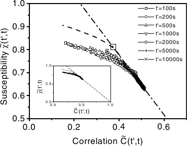
Figure 9.4: Violation of the fluctuation-dissipation theorem (dotted-dashed line) in an experimental spin glass (from [herisson:02], see text for discussion). In the figure, $t^{\prime}$ corresponds to our $t_{\mathrm{w}}$ and $t$ corresponds to our $t+t_{\mathrm{w}}$.

A good example of the relevance of these predictions for experimental work is the case of the mild violations of the classic fluctuation-dissipation theorem (FDT). This result, proven in [callen:51, kubo:57], makes it possible to predict the system’s response to an external field from its equilibrium dynamics, but only if the system was already in equilibrium when the field was applied. Still, the pattern of violations of the FDT for spin glasses admits a very simple parameterisation. Cugliandolo and Kurchan [cugliandolo:94b, cugliandolo:97] proposed characterising the deviations from the FDT behaviour by studying a fluctuation-dissipation ratio, representing the response as a function of the system correlations.

This procedure was followed experimentally in [herisson:02] and the result is represented in Figure 9.4. In it, the authors consider the response function at time $t+t_{\mathrm{w}}$ of a field that was switched off at time $t_{\mathrm{w}}$, denoted by $\tilde{\chi}(t,t_{\mathrm{w}})$. This is represented against the temporal autocorrelation of the system $\tilde{C}(t,t_{\mathrm{w}})$. Should the systems obey FDT, the resulting plot $\tilde{\chi}(\tilde{C})$ should fall on a straight line (dotted-dashed line in the figure). In the spin glass, the linear behaviour is indeed reproduced for short measuring times $t$, but the curves eventually deviate from this prediction at a $t_{\mathrm{w}}$-dependent branching point.

In the $t_{\mathrm{w}}\to\infty$ limit, the RSB and droplet pictures expect a different pattern of violations. In both theories, the measured curved should branch off from the FDT prediction at $\tilde{C}=q_{\text{EA}}$. However, in the RSB framework one expects that $\lim_{t_{\mathrm{w}}\to\infty}\mathrm{d}\tilde{\chi}/\mathrm{d}\tilde{C}$ would correspond to the Parisi function $x(q)$ that we introduced in Section 9.2.1 [franz:98, franz:99]. In the droplet picture, on the other hand, the curve of violations should be horizontal. In Figure 9.4 the authors have attempted this extrapolation (dashed line).

9.3  The Edwards-Anderson spin-glass in numerical simulations

In order to be made quantitative, the different theories for the spin-glass phase need input from numerical simulations. In this sense one can take two complementary approaches

• Simulate a very large system with a Monte Carlo update that reproduces the physical evolution (such as heat bath or Metropolis dynamics). As long as $\xi(t_{\mathrm{w}})\ll L$, one can consider to be observing the same thermodynamical-limit behaviour as in a physical sample. Then, take a long-$t_{\mathrm{w}}$ limit to predict the physical evolution.

• Simulate smaller lattices with some kind of optimised dynamics (typically parallel tempering) to equilibrate the systems. Then perform a finite-size scaling study to perform a large-$L$ extrapolation. Use the information thus obtained on the equilibrium spin-glass phase to predict the experimental non-equilibrium behaviour.

We stress that the goal of numerical work on the Edwards-Anderson model is ultimately to understand the nature of the spin-glass phase. In this sense, the situation is complementary to that of the DAFF. In the latter, the low-temperature phase is trivial (antiferromagnetic order), but the phase transition itself is poorly understood. In the spin glass, the phase transition has been thoroughly examined numerically [palassini:99, ballesteros:00, hasenbusch:08, hasenbusch:08b], and it is the low-temperature phase, as far from the critical point as possible, that has the most interest.

Of course, the extreme sluggishness of the dynamics poses a problem for numerical investigations. For instance, the typical time scales of experiments on spin glasses range from a few seconds to a few hours, but each MCS is equivalent to only $10^{-12}$ s [mydosh:93]. Therefore, one has to perform an enormous number of lattice updates even to begin to approach the physically relevant regime. In this sense, non-equilibrium simulations have reached only about $10^{-4}$ s. In the equilibrium case, the lattice sizes that one can thermalise are very small, so the data are always suspect of being dominated by finite-size effects and not considered representative of the real physics.

On the other hand, the understanding of the spin-glass phase is not yet ripe for a tethered study, because the appropriate reaction coordinate (which must be sample-dependent) is not known. Still, some of the techniques developed in the previous chapters will prove to be useful.

9.3.1 Introduction to our work with Janus

In the following chapters we shall take a brute-force approach to the numerical study of the spin-glass phase. In particular, we have carried out our simulations using Janus, a special-purpose machine optimised for Monte Carlo simulations of spin systems. For this restricted class of problems, Janus can outperform conventional computing architectures by several orders of magnitude, thus providing a qualitative jump in the time and length scales that can be accessed. In particular, we have been able to follow the non-equilibrium dynamics up to times of $0.1$ s, at the threshold of the experimental scale, and we have thermalised lattices up to $L=32$ down to $T=0.64T_{\text{c}}$.

The characteristics of Janus are very briefly explained in Appendix D. The Ising spin-glass simulations carried out with Janus, whose parameters we report in Appendix E, have produced four physics publications so far: [janus:08b, janus:09b, janus:10, janus:10b]. This work is the fruit of the collaboration of a large number of people, including physicists and engineers. To reflect this, the following chapters include only those physical studies where the author carried out a major fraction of the work. In particular, we leave out the results corresponding to Sections 5.2 and 6 in [janus:09b], as well as those corresponding to Sections 7.2 and 7.3 in [janus:10]. Fortunately, the quoted sections are relatively independent from the rest of the works, so our presentation will be self-contained.

We note that the order of presentation of our results in this and the next chapter is markedly different from their original development. In our original work we were of course constrained by the running of the simulations (we carried out the non-equilibrium ones first, while our equilibrium simulation campaign took over a year). In this dissertation, we shall try to present the results in a logical fashion, rather than in a chronological one.

CHAPTER X   The statics-dynamics correspondence and the finite-time scaling paradigm

In this chapter we tackle the second of our main topics: the relation between the (experimentally unreachable) equilibrium phase and the off-equilibrium dynamics in the context of spin glasses.

After introducing the relevant physical observables and correlation functions, we try to characterise the isothermal aging dynamics of the $D=3$ Edwards-Anderson spin-glass. We begin by using only non-equilibrium simulations and study issues like the growing characteristic lengths or the thermoremanent magnetisations.

Eventually, however, the non-equilibrium study faces an imposing stumbling block: in order fully to understand the reasons for the dynamical behaviour at finite time one must consider extrapolations to infinite time. In particular, we observe a very interesting crossover behaviour in the so-called dynamical heterogeneities (Section 10.5) that we will be unable to quantify.

It is then that we introduce a complementary approach: that of finite-size equilibrium simulations. First, we promote the relation between the equilibrium phase and the dynamics to a quantitative level, through a time-length dictionary. This will allow us to introduce one of the most important concepts (and results) of this study: the notion that experimental non-equilibrium physics is equivalent to the equilibrium behaviour, not of the thermodynamical limit, but of a more modest lattice of $L\sim 100$.

Finally, we resume the analysis of dynamical heterogeneities from an equilibrium point of view. This allows us to perform a fully quantitative study and, through it, to take the statics-dynamics one step further: the finite-time scaling paradigm.

Throughout this chapter, we shall focus only on those aspects of the spin-glass dynamics and equilibrium about which the different theoretical pictures are in full agreement. For instance, we do not try to decide whether the dynamics is coarsening-like or not. We shall see that this neutral approach can actually take us very far.

In Chapter 11 we shall, on the other hand, address the RSB-droplet-TNT controversy directly. We shall then try to decide which of these is a better description of the spin-glass phase.

10.1  Physical observables for spin-glass dynamics

We work on the Edwards-Anderson model introduced in the previous chapter,

$$\mathcal{H}=-\sum_{\langle{\boldsymbol{x}},{\boldsymbol{y}}\rangle}J_{{\boldsymbol{x}}{\boldsymbol{y}}}s_{\boldsymbol{x}}s_{\boldsymbol{y}}.$$ (9.6)

We use bimodal couplings, $J_{{\boldsymbol{x}}{\boldsymbol{y}}}=\pm 1$ with $50\%$ probability. For this Hamiltonian, the phase transition occurs at $T_{\mathrm{c}}=1.109(10)$ [hasenbusch:08, hasenbusch:08b].

We study the dynamics in the direct quench protocol explained in the previous chapter. We use heat-bath dynamics, which is in the universality class of physical evolution. We take $1$ MCS to correspond to $10^{-12}$ seconds [mydosh:93]. When studying the non-equilibrium dynamics we shall consider that we are in the thermodynamical limit, even if we simulate in a finite lattice ($L=80$ in our case). In practice, this approximation is good as long as the length scale of the coherent domains that grow during the evolution remains much smaller than the system size. We shall check this issue in Section 10.3.2

We represent by $O(t_{\mathrm{w}})$ the time evolution of some observable $O$ for a single sample, and by $\overline{O(t_{\mathrm{w}})}$ its disorder average. In principle one would have to average over many thermal histories. However, the main source of error is sample-to-sample fluctuation, so it is better to run more samples than more histories for each one. Still, we run two independent thermal histories for each sample (two real replicas), for reasons that will become apparent below. Whenever one observable can be averaged over the two replicas, we shall do so, even if we do not indicate it explicitly.

The first issue we have to consider when defining physical observables is the gauge symmetry induced by the quenched average [toulousse:77]. Indeed, the Hamiltonian is unchanged under the transformation

$$s_{\boldsymbol{x}} \longrightarrow\alpha_{\boldsymbol{x}}s_{\boldsymbol{x}},$$ (10.1)

$$J_{{\boldsymbol{x}}{\boldsymbol{y}}} \longrightarrow\alpha_{\boldsymbol{x}}J_{{\boldsymbol{x}}{\boldsymbol{y}}}\alpha_{\boldsymbol{y}},$$ (10.2)

where $\alpha_{\boldsymbol{x}}=\pm 1$. In principle, this would mean that one should have to consider for each observable its gauge average $2^{-L^{D}}\sum_{\{\alpha_{\boldsymbol{x}}\}}O(\{\alpha_{\boldsymbol{x}}s_{\boldsymbol{x}}\})$. Notice, however, that the gauge-transformed couplings are as probable as the original ones, so the disorder average of $O$ is the same as its average over the gauge orbit.

We need, therefore, gauge invariant observables. The usual way out of this problem is introducing real replicas. These are defined as statistically independent systems $\{s^{(i)}_{\boldsymbol{x}}\}$ that evolve with the same set of $J_{{\boldsymbol{x}}{\boldsymbol{y}}}$. Their overlap field is

$$q_{\boldsymbol{x}}=s_{\boldsymbol{x}}^{(1)}(t_{\mathrm{w}})s_{\boldsymbol{x}}^{(2)}(t_{\mathrm{w}}),$$ (10.3)

obviously gauge-invariant.

The averaged density of the overlap field defines the spin-glass order parameter, the spin overlap $q$

$$q(t_{\mathrm{w}})=\frac{1}{N}\sum_{\boldsymbol{x}}q_{\boldsymbol{x}}(t_{\mathrm{w}}).$$ (10.4)

We can also consider the spin-glass susceptibility

$$\chi_{\text{SG}}(t_{\mathrm{w}})=N\overline{q^{2}(t_{\mathrm{w}})},$$ (10.5)

which, as can be seen using fluctuation-dissipation relations, is essentially the same as the non-linear susceptibility $\chi_{4}$ —see (5.4) and (5.23). In fact (in equilibrium)

$$6\chi_{4}=\chi_{\text{SG}}-2/3.$$ (10.6)

10.1.1 Temporal correlations

Since we are working on an aging system, we need to consider two time scales, as we commented in Chapter 9. We are particularly interested in the overlap between the configurations at the waiting time $t_{\mathrm{w}}$ and at the measuring time $t+t_{\mathrm{w}}$,

$$c_{\boldsymbol{x}}(t,t_{\mathrm{w}})=s_{\boldsymbol{x}}^{(i)}(t_{\mathrm{w}})s_{\boldsymbol{x}}^{(i)}(t+t_{\mathrm{w}}).$$ (10.7)

Notice that this quantity needs only one replica.

We can use the two-time overlap to define the temporal correlation function

$$C(t,t_{\mathrm{w}})=\overline{\frac{1}{N}\sum_{\boldsymbol{x}}c_{\boldsymbol{x}}(t,t_{\mathrm{w}})}.$$ (10.8)

For fixed $t_{\mathrm{w}}$, $C(t,t_{\mathrm{w}})$ is strictly decreasing in $t$, indicating the gradual but very slow decorrelation in the system. In fact, for fixed $t_{\mathrm{w}}$, the $C(t,t_{\mathrm{w}})$ can be interpreted as the thermoremanent magnetisation (Section 10.4). This is because we can make a gauge transformation from the uniform configuration resulting from a strong magnetic field to the random initial configuration in our simulations. Therefore, the overlap with this random configuration plays the part of a magnetisation.

In the pseudoequilibrium regime, $t\ll t_{\mathrm{w}}$, the (real part of the) magnetic susceptibility at frequency $\omega=2\uppi/T$ is given by the fluctuation-dissipation formula $\bigl{(}1-C(t,t_{\mathrm{w}})\bigr{)}/T$.

For any finite $t_{\mathrm{w}}$, $\lim_{t\to\infty}C(t,t_{\mathrm{w}})=0$. However, in equilibrium $t_{\mathrm{w}}\to\infty$, the overlap has a finite value below $T_{\mathrm{c}}$. In particular, if we define the stationary, or translationally invariant, part of the correlation,

$$C_{\infty}(t)=\lim_{t_{\mathrm{w}}\to\infty}C(t,t_{\mathrm{w}}),$$ (10.9)

we get

$$q_{\text{EA}}=\lim_{t\to\infty}C_{\infty}(t).$$ (10.10)

This equation defines the value of the Edwards-Anderson order parameter. The dynamical computation of $q_{\text{EA}}$ from this limit is notoriously difficult [perez-gaviro:06, iniguez:97], even with the extremely long times simulated on Janus (Section 10.6). In this chapter, we shall consider an alternative, equilibrium, approach (Section 10.8).

The introduction of the stationary part of $C(t,t_{\mathrm{w}})$ can be generalised to a division of this correlation function in several time sectors. We can define the $\mu$ sector by

$$C_{\infty}^{(\mu)}(s)=\lim_{t_{\mathrm{w}}\to\infty}(st^{\mu}_{t_{\mathrm{w}}},t_{\mathrm{w}}).$$ (10.11)

The translationally invariant sector would thus correspond to $\mu=0$. Notice that $q_{\text{EA}}<C^{(0)}_{\infty}(s)<1$. In order to cover the whole range of values $C\in[0,1]$, at least another sector must be considered. The simplest (and experimentally supported) one is the full-aging regime [rodriguez:03], obtained by setting $\mu=1$. If full-aging holds, one would expect $C^{(1)}_{\infty}(s)$ to cover the whole range from $q_{\text{EA}}$ to $0$. We shall examine these claims in Section 10.2.

We finally note that some authors [castillo:02, castillo:03] use different definitions for these functions, so care must be exercised when consulting the literature. In particular, often $t$ is taken to be our $t+t_{\mathrm{w}}$ and the $C_{\infty}(t)$ is defined so that it tends to zero (i.e., subtracting $q_{\text{EA}}$ from it).

10.1.2 Spatial correlations

The spin-glass dynamics is characterised by the growth of coherent domains both in the coarsening and the non-coarsening pictures (even if their shape and nature differ). These can be studied through the spatial autocorrelation of the overlap field

$$C_{4}(\boldsymbol{r},t_{\mathrm{w}})=\overline{\frac{1}{N}\sum_{\boldsymbol{x}}q_{\boldsymbol{x}}(t_{\mathrm{w}})q_{{\boldsymbol{x}}+\boldsymbol{r}}(t_{\mathrm{w}})}\ .$$ (10.12)

In particular, the long-distance decay of $C_{4}(\boldsymbol{r},t_{\mathrm{w}})$ defines the coherence length $\xi(t_{\mathrm{w}})$

$$C_{4}(\boldsymbol{r},t_{\mathrm{w}})\xrightarrow{\ \ r\to\infty\ \ }\frac{1}{r^{a}}f\bigl{(}r/\xi(t_{\mathrm{w}})\bigr{)}.$$ (10.13)

At the critical point, $a$ is non-zero and related to the anomalous dimension, through $a(T_{\mathrm{c}})=D-2+\eta$. In $D=3$, $a(T_{\mathrm{c}})=0.625(10)$ [hasenbusch:08, hasenbusch:08b].

Below $T_{\mathrm{c}}$, the value of $a$ characterises the dynamics. For fixed $r/\xi(t_{\mathrm{w}})$, the correlation function of a coarsening system does not tend to zero when $r\to\infty$, since the domains are compact. In a system described by the RSB picture, however, there exist equilibrium states with $q=0$, so the dynamics remains forever with a vanishing order parameter. This is related to the existence of the replicon mode, a Goldstone boson (like magnons in Heisenberg ferromagnets or pions in high-energy physics). Therefore, $a\neq 0$ for RSB systems. It has been conjectured that $a(T<T_{\mathrm{c}})=a(T_{\mathrm{c}})/2$ [dedominicis:98]. The exponent $a$ is probably discontinuous at $T_{\mathrm{c}}$ [parisi:97].

In short, the value of $a$ below the critical temperature is a good marker to distinguish coarsening dynamics (droplet or TNT) from the RSB predictions. We shall consider this issue in Chapter 11.

Notice that the presence of the damping function is required due to causality considerations. In the case of $C_{4}(\boldsymbol{r},t_{\mathrm{w}})$, the damping function $f$ seems to decay a little faster than an exponential [jimenez:05, marinari:00b],

$$f(x)\sim e^{-x^{\beta}},\qquad\beta\approx 1.5.$$ (10.14)

Notice that the spin-glass susceptibility (10.5) can be defined as

$$\chi_{\text{SG}}(t_{\mathrm{w}})=N\overline{q^{2}(t_{\mathrm{w}})}=\int\mathrm{d}^{D}\boldsymbol{r}\ C_{4}(\boldsymbol{r},t_{\mathrm{w}}).$$ (10.15)

In order to characterise the aging dynamics, one must take dynamical heterogeneities into account [castillo:02, castillo:03, jaubert:07]. This is best accomplished through the two-time spatial correlation

$$C_{2+2}(\boldsymbol{r},t,t_{\mathrm{w}})=\overline{\frac{1}{N}\sum_{\boldsymbol{x}}\bigl{[}c_{\boldsymbol{x}}(t,t_{\mathrm{w}})c_{{\boldsymbol{x}}+\boldsymbol{r}}(t,t_{\mathrm{w}})-C^{2}(t,t_{\mathrm{w}})\bigr{]}}$$ (10.16)

Notice that this is a connected correlation function. In principle, it may seem more natural to subtract $\overline{C(t,t_{\mathrm{w}})}^{2}$, but due to the self-averaging nature of $C$ (see below), both definitions are equivalent in the thermodynamical limit. We note that this correlation is natural for the structural glasses problem, where the order parameter is not known (see, e.g., [berthier:05] and references therein).

$C_{2+2}$ seems complicated, but it actually has a simple probabilistic interpretation. Let us call a defect a site where $c_{\boldsymbol{x}}(t,t_{\mathrm{w}})=-1$ and let $n(t,t_{\mathrm{w}})$ be the density of such defects. Trivially, $C(t,t_{\mathrm{w}})=1-2n(t,t_{\mathrm{w}})$. Then, the conditional probability of finding a defect at site ${\boldsymbol{x}}+\boldsymbol{r}$, knowing that there is one at ${\boldsymbol{x}}$, is $n(t,t_{\mathrm{w}})g(\boldsymbol{r})$, where $g(\boldsymbol{r})$ represents the pair-correlation function of the defects. Hence, $C_{2+2}(\boldsymbol{r},t,t_{\mathrm{w}})$ is just $4n^{2}(t,t_{\mathrm{w}})\bigl{(}1-g(\boldsymbol{r})\bigr{)}$.

The long-distance decay of $C_{2+2}(\boldsymbol{r},t,t_{\mathrm{w}})$ defines the correlation length $\zeta(t,t_{\mathrm{w}})$, the characteristic length scale for dynamic heterogeneities,

$$C_{2+2}(\boldsymbol{r},t,t_{\mathrm{w}})\xrightarrow{\ \ r\to\infty\ \ }\frac{1}{r^{b}}g\bigl{(}r(\zeta(t,t_{\mathrm{w}})\bigr{)}\ .$$ (10.17)

Little is known in the literature about either $b$ of $g$, since, before Janus, the time scales that could be explored reached only very small values of $\zeta(t,t_{\mathrm{w}})$.

Notice that we have called $\zeta$ a correlation length, while we said that $\xi$ was a coherence length. The distinction stems from the fact that the former is computed from a connected correlation function and the latter from a non-connected one. In particular, $\xi(t_{\mathrm{w}})$ diverges in the large-$t_{\mathrm{w}}$ limit, while this may or may not be the case for $\zeta$. We must point out, though, that this nomenclature is not universal.

In the RSB framework, we can distinguish two sectors in the dynamics: (i) relaxation within a single state, where $q_{\text{EA}}<C<1$, and (ii) exploration of new states, where $C<q_{\text{EA}}$. These can be identified by the relation of $\zeta$ and $\xi$. In particular, for sector (i) we expect $\zeta(t,t_{\mathrm{w}})\ll\xi(t_{\mathrm{w}})$. We shall find $\zeta(t,t_{\mathrm{w}})/\xi(t_{\mathrm{w}})$ a valuable dynamical variable (Section 10.9).

Throughout this chapter, and the next, we shall need to consider the evolution of the physical observables along many orders of magnitude in time, which complicates their interpretation and analysis. Yet, recall that, for fixed $t_{\mathrm{w}}$, $C(t,t_{\mathrm{w}})$ defines a one-to-one relation between $C$ and $t$. Hence, we shall often eliminate $t$ as an independent variable in favour of $C$.

A final note concerns the issue of self-averaging. Notwithstanding the discussion in Section 2.2.2, most of the observables considered here are actually self-averaging. This is because, in the non-equilibrium regime, the coherence length is much smaller than $L$, so we essentially have about $L^{D}/\xi^{D}$ independent blocks. The exception is $\chi_{\text{SG}}$, which is non-local. In fact, the central limit theorem suggests that the probability distribution of $q(t_{\mathrm{w}})$ should tend to a Gaussian when $L\to\infty$. Therefore, the variance of $\chi_{\text{SG}}(t_{\mathrm{w}})$ is $\sim 2\chi_{\text{SG}}^{2}(t_{\mathrm{w}})$ in the limit of large systems.

10.1.3 Our non-equilibrium simulations

We comment the parameters of our non-equilibrium simulations, as well as some technical details, in Appendix E. Let us summarise by saying that we have run simulations for three subcritical temperatures $T=0.6,0.7,0.8$ as well as for $T=1.1\approx T_{\mathrm{c}}$. For the first three temperatures, we reached $t_{\mathrm{w}}=10^{11}$, simulating $96$ samples for $T=0.6,0.8$ and $63$ samples for $T=0.7$. At the critical point we reached $t_{\mathrm{w}}=4.2\times 10^{9}$ and simulated $32$ samples.

These simulations were first presented in [janus:08b]. Later, in [janus:09b], we simulated a new set of $768$ samples for $T=0.7$, which shall constitute our main working temperature. For these new simulations we reached only $t_{\mathrm{w}}=10^{10}$, since for longer times we had observed finite-size effects (see Section 10.3.2). When discussing our results at $T=0.7$, we shall find it sometimes convenient to use the longer $63$-sample simulation, instead of the shorter but more precise one with $768$ samples.

10.2  Aging and full aging in $C(t,t_{\mathrm{w}})$

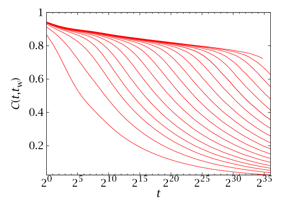
Figure 10.1: Temporal correlation function $C(t,t_{\mathrm{w}})$, Eq. (10.8), for $T=0.6$. We plot the curves as a function of $t$ for $t_{\mathrm{w}}=2^{2i}$, where $i=1,2,\ldots,18$ ($t_{\mathrm{w}}$ grows from bottom to top). The errors are smaller than the width of the lines.

We start our study of the non-equilibrium dynamics by considering the two-time correlation function. In Figure 10.1 we have plotted $C(t,t_{\mathrm{w}})$ for $T=0.6$ (our lowest temperature), for a range of $t_{\mathrm{w}}$ across $11$ orders of magnitude (equivalent to physical times from picoseconds to one tenth of a second).

We observe the qualitative claims made in the previous section, namely

• For each $t_{\mathrm{w}}$, $C(t,t_{\mathrm{w}})$ is a strictly decreasing function of $t$.

• $\lim_{t\to\infty}C(t,t_{\mathrm{w}})=0$.

• As we increase $t_{\mathrm{w}}$, we begin to see an enveloping curve. This is the $C_{\infty}(t)$ that we shall study in Section 10.6.

In the following we try to quantify these remarks. We begin by attempting to parameterise the aging behaviour. It has been claimed in experimental work [rodriguez:03] that $C(t,t_{\mathrm{w}})$ is well described by a full-aging behaviour, that is

$$C(t,t_{\mathrm{w}})=f\bigl{(}(t+t_{\mathrm{w}})/t_{\mathrm{w}}\bigr{)},$$ (10.18)

at least in the range $10^{14}<t_{\mathrm{w}}<10^{16}$. To check for this in a systematic way, we consider the functional form

$$C(t,t_{\mathrm{w}})=A(t_{\mathrm{w}})(1+t/t_{\mathrm{w}})^{-\alpha(t_{\mathrm{w}})}.$$ (10.19)

If full aging is correct, the parameters $A(t_{\mathrm{w}})$ and $\alpha(t_{\mathrm{w}})$ should be constant for large $t_{\mathrm{w}}$. This has been checked before [jimenez:03], but with much smaller statistics.

We present the results of fits to (10.19) as a function of $t_{\mathrm{w}}$ for our three subcritical temperatures of $T=0.6,0.7,0.8$ in Figure 10.2. For each $t_{\mathrm{w}}$, we consider the range $t_{\mathrm{w}}\leq t\leq 10t_{\mathrm{w}}$ (we want to avoid the short-times behaviour). These fits, and their errors, have been computed with the jackknife method explained in Appendix B. In our simulated range, the exponent $\alpha(t_{\mathrm{w}})$ is an increasing function of $t_{\mathrm{w}}$, but its growth slows down noticeably. Still, the behaviour at $t_{\mathrm{w}}=10^{16}$ seems beyond reasonable extrapolation.

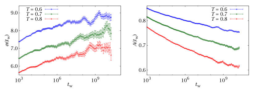
Figure 10.2: Parameters in a fit of $C(t,t_{\mathrm{w}})$ to (10.19) as functions of $t_{\mathrm{w}}$. For $T=0.7$ we use our longer simulations with $63$ samples (cf. Figure b.3). The evolution seems to slow down for large $t_{\mathrm{w}}$, but we do not yet see the full aging behaviour, in which these parameters are constant.

Notice that the $\alpha(t_{\mathrm{w}})$ exhibits some suspicious undulations (especially for $T=0.6$). This is a visual effect caused by the data correlation, as we discuss in detail in Section B.3.3.2.

In Section 10.4 we shall use our fits to (10.19) to study the thermoremanent magnetisation.

10.3  Spatial correlations and the coherence length

In this section we consider the issue of growing length scales in the spin-glass dynamics. The computation of characteristic length scales is a recurring problem in statistical mechanics, as well as in lattice gauge theory. In previous chapters we solved it by considering the second-moment definition (5.9). Notice that, in the thermodynamical limit, this second-moment estimator is equivalent to

$$\xi_{2}^{(\infty)}=\sqrt{\frac{\int\mathrm{d}^{D}\boldsymbol{r}\ \boldsymbol{r}^{2}C_{4}(\boldsymbol{r},t_{\mathrm{w}})}{\int\mathrm{d}^{D}\boldsymbol{r}\ C_{4}(\boldsymbol{r},t_{\mathrm{w}})}}\ .$$ (10.20)

The denominator in this equation is $\chi_{\text{SG}}(t_{\mathrm{w}})$, Eq. (10.15), which does not self-average. Therefore, this method is problematic in non-equilibrium studies, where one considers very large systems but not many samples (in our case ${\mathcal{N}}_{\text{samples}}\approx 100$ for $T=0.6,0.8,T_{\mathrm{c}}$ and ${\mathcal{N}}_{\text{samples}}=768$ for $T=0.7$).

On the face of this problem, one could think of replacing the integral estimators by fits to some functional form for $C_{4}(\boldsymbol{r},t_{\mathrm{w}})$ featuring the $\xi(t_{\mathrm{w}})$. However, in the spin-glass case we do not know this explicit functional form —we have at best a reasonable ansatz as to its scaling, Eq. (10.13)— so this is not a viable alternative. In addition, we would face the ever present problem of statistical correlations, which complicate fits and their interpretation.

Therefore, we must go back to the integral estimators. In this respect notice that the $C_{4}(\boldsymbol{r},t_{\mathrm{w}})$, for fixed $\boldsymbol{r}$, is self-averaging. The lack of self-averaging in $\xi_{2}$ stems from the fact that the integration volume grows with $L$. For a fixed size, it is the dismal signal-to-noise ratio in the long-distance tails which spoils the precision. But this is precisely the problem that one faces when trying to compute the integrated autocorrelation time from a time series (Section A.2.1) and we can borrow its solution: a self-consistent cutoff.

10.3.1 Integral estimators of characteristic length scales

We start our discussion by simplifying our definition of the spatial correlations to take into account only values of $\boldsymbol{r}$ along the axes. We define

$$C_{4}(r,t_{\mathrm{w}})=\frac{1}{D}\sum_{i=1}^{D}C_{4}(r\hat{\boldsymbol{u}}_{i},t_{\mathrm{w}}),$$ (10.21)

where the $\hat{\boldsymbol{u}}_{i}$ denote each of the lattice unit vectors. That is, we take the values of the correlation for a distance $r$ along the axes as representative of the whole spherical shell of radius $r$. We shall study the goodness of this approximation in Section 10.3.4,

Now, for positive integer $k$, we consider the integral,

$$I_{k}(t_{\mathrm{w}})=\int_{0}^{L/2}\mathrm{d}r\ r^{k}C_{4}(r,t_{\mathrm{w}}).$$ (10.22)

Notice that our bound of integration is $L/2$, and not $L$, due to the periodic boundary conditions. Since we are considering the regime $\xi(t_{\mathrm{w}})\ll L$, this makes no difference. In addition, the actual numerical computation of $I_{k}$ uses an error-dependent cutoff: we only integrate up to the point $r_{\text{cutoff}}$ where the relative error in $C_{4}(r,t_{\mathrm{w}})$ rises above some threshold. This is the same trick used in the computation of the integrated autocorrelation time in Section A.2.1. We shall discuss this issue in more detail in Section 10.3.3.

With this notation, and assuming rotational invariance, the second-moment estimate is

$$\xi^{(\infty)}_{2}\simeq\sqrt{\frac{I_{D+1}(t_{\mathrm{w}})}{I_{D-1}(t_{\mathrm{w}})}}\ .$$ (10.23)

An alternative approach, considered in [kisker:96], would be to identify $\xi(t_{\mathrm{w}})$ with $I_{0}(t_{\mathrm{w}})$, which has the correct dimensions. However, this is only a good definition if $a=0$ and we want a definition that would work for any scaling behaviour of the type (10.13). To this end, we note first that

$$I_{k}(t_{\mathrm{w}})\propto\xi^{k+1-a}(t_{\mathrm{w}}).$$ (10.24)

Therefore, we can introduce the following definition

$$\xi_{k,k+1}(t_{\mathrm{w}})=\frac{I_{k+1}(t_{\mathrm{w}})}{I_{k}(t_{\mathrm{w}})}\propto\xi(t_{\mathrm{w}}).$$ (10.25)

Notice that the coherence length is only defined up to a constant scale factor, so any of the $\xi_{k,k+1}(t_{\mathrm{w}})$ would work.

Still, there is a systematic error involved. Equation (10.13) is valid only in the regime where $1\ll r\ll L$. The resulting bias is minimised by considering large values of $k$, which suppress short distances in the integrals. However, too large a value of $k$ would give too much weight to the tails of the correlation function, where the signal-to-noise ratio is worst. A compromise in the value of $k$ is clearly needed (cf. Figure 10.5).

In Section 10.3.3 we shall compare different estimators of the coherence length and demonstrate that, indeed, the integral ones produce a significant error reduction. Furthermore, the issue of the choice of $k$ is not as critical as it may seem. For the moment, let us proceed with the physical discussion, using as our preferred estimator $\xi_{1,2}(t_{\mathrm{w}})$.

10.3.2 The dynamical critical exponent and finite-size effects

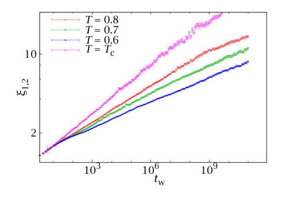
Figure 10.3: Growth of the coherence length for several subcritical temperatures and for the critical point. For $T=0.7$ we use our longer simulations with $63$ samples.

We consider in Figure 10.3 our coherence length $\xi_{1,2}(t_{\mathrm{w}})$ for $T=T_{\mathrm{c}}$ and for our three subcritical temperatures. For $T=0.7$ we have plotted our simulations with $63$ samples, since they reach longer times.

As expected, the growth of $\xi(t_{\mathrm{w}})$ is slower at lower temperatures. Furthermore, our curves follow a power law for a wide time range. There are some deviations at short times, due to lattice discretisation effects (our definitions do not make much sense for $\xi\lesssim 3$). Some of the curves also present some deviations for long times (this is most noticeable for $T=0.8$).

These can be interpreted as finite-size effects, even though we are simulating very large lattices ($L=80$). Indeed, when studying non-equilibrium dynamics we assume that our system is in the thermodynamical limit, which in principle requires $\xi(t_{\mathrm{w}})\ll L$. In practice, the bound depends on the numerical accuracy. From finite-size scaling we would expect the largest $t_{\mathrm{w}}$ for which $L=80$ still represents $L=\infty$ physics to scale as $L\geq k\xi_{1,2}(t_{\mathrm{w}})$. We have estimated $k$ by computing $\xi_{1,2}(t_{\mathrm{w}})$ in simulations for $L=24,40$ and noting where they diverge from their $L=80$ counterparts (Figure 10.4). We conclude that at $T=0.8$ the safe range is $L\geq 7\xi_{1,2}(t_{\mathrm{w}})$. For $T_{\mathrm{c}}$, the equivalent bound is $L\geq 6\xi_{1,2}(t_{\mathrm{w}})$.

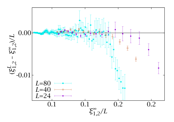
Figure 10.4: Finite size effects in $\xi(t_{\mathrm{w}})$, obtained by computing the difference between $\xi_{1,2}(t_{\mathrm{w}})$ for each of our lattice sizes and a power-law extrapolation. In particular, we define $\xi^{\infty}_{1,2}(t_{\mathrm{w}})$ as the result of applying the fit to (10.26), computed for $L=80$ in the range $\xi\in[3,10]$, to the whole temporal range. Then, for each lattice size we consider the relative difference $[\xi_{1,2}^{\infty}(t_{\mathrm{w}})-\xi_{1,2}^{(L)}(t_{\mathrm{w}})]/\xi_{1,2}^{\infty}(t_{\mathrm{w}})$.

$T$	${\mathcal{N}}_{\text{samples}}$	$[\xi_{\text{min}},\xi_{\text{max}}]$	$z$	$\chi^{2}_{\text{d}}$/d.o.f.	$t_{\mathrm{w}}^{\text{max}}$
$0.6$	96	$[3,10]$	14.06(25)	41.7/82	$\approx 9\times 10^{11}$
$0.7$	63	$[3,10]$	11.84(22)	82.7/81	$\approx 2.2\times 10^{10}$
		$[3.5,10]$	12.03(27)	52.7/71
$0.8$	96	$[3,10]$	9.42(15)	17.1/63	$\approx 4.3\times 10^{8}$
$1.1$	32	$[3,10]$	6.86(16)	18.7/46	$\approx 3.5\times 10^{6}$
$0.7$	768	$[3,10]$	11.45(10)	86.9/76	$\approx 2.2\times 10^{10}$
		$[3.5,10]$	11.56(13)	46.6/66
		$[4,10]$	11.64(15)	40.1/58
		$[4.5,10]$	11.75(20)	29.6/50

Table 10.1: Value of the dynamic critical exponent $z$ for several temperatures. For our simulations with less than $100$ samples we have used the fitting range $\xi_{1,2}\in[3,10]$, while for our $768$-sample simulation at $T=0.7$ we have needed to restrict the fitting range. For $\xi_{1,2}(t_{\mathrm{w}})>10$, our simulations are affected by finite-size effects. We also report the value of $t_{\mathrm{w}}^{\text{max}}$ for which this bound is reached (for $T=0.6$ we never reach $\xi_{1,2}=10$, so this is an extrapolation).

In order to be safe, we have considered that $\xi_{1,2}(t_{\mathrm{w}})$ is physically meaningful for $3\leq\xi(t_{\mathrm{w}})\leq 10$. For $T=0.6$ the upper bound is not reached, while for $T=0.7$ it corresponds to $t_{\mathrm{w}}\sim 10^{10}$ and for $T=0.8$ it corresponds to $t_{\mathrm{w}}\sim 10^{8}$. In this range, we have fitted the coherence length to a power law, in order to determine the dynamical critical exponent $z$,

$$\xi(t_{\mathrm{w}})=A(T)t_{\mathrm{w}}^{1/z(T)}\ .$$ (10.26)

The results of these fits can be seen in Table 10.1. We also include the maximum waiting time safe from finite-size effects, defined as $\xi_{1,2}(t_{\mathrm{w}}^{\text{max}})=10$.

The resulting values of $z$ are very large, going from $z(T_{\mathrm{c}})=6.86(16)$ at the critical point to $z(T=0.6)=14.06(25)$ at our lowest temperature. Also, we find that this exponent roughly follows the law

$$z(T)=z(T_{\mathrm{c}})\frac{T_{\mathrm{c}}}{T}\,,$$ (10.27)

consistent with previous numerical and experimental studies [joh:99, marinari:00b].

Furthermore, if we extrapolate the coherence length to a typical experimental scale of $100$ s ($t_{\mathrm{w}}\sim 10^{14}$), we find

$$\xi_{1,2}(t_{\mathrm{w}}=10^{14},T=0.6) =14.0(3),$$ (10.28)

$$\xi_{1,2}(t_{\mathrm{w}}=10^{14},T=0.7) =21.7(4),$$ (10.29)

$$\xi_{1,2}(t_{\mathrm{w}}=10^{14},T=0.8) =37.0(14),$$ (10.30)

$$\xi_{1,2}(t_{\mathrm{w}}=10^{14},T=T_{\mathrm{c}}\ ) =119(9),$$ (10.31)

which nicely compare with experiments [joh:99, bert:04].

10.3.3 Comparison of different estimators of the coherence length

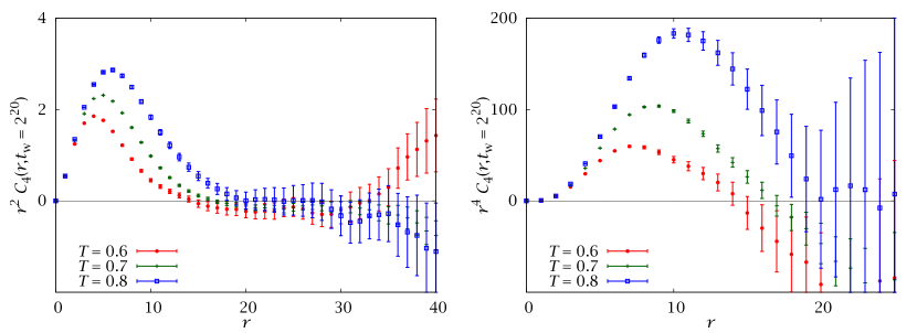
Figure 10.5: Plot of the spatial correlation function $C_{4}(r,t_{\mathrm{w}})$ for several subcritical temperatures and $t_{\mathrm{w}}=2^{20}$. We show the correlation multiplied by $r^{2}$ (left) and $r^{4}$ (right), needed to compute $I_{2}(t_{\mathrm{w}})$ and $I_{4}(t_{\mathrm{w}})$, respectively. The signal-to-noise ratio is the same in both cases, but for the latter the distances with maximum weight are closer to the noise-dominated region. The curve for $T=0.7$ is the average over $768$ samples, while those for $T=0.6,0.8$ were computed with $96$ samples.

In this section we consider some details on the implementation of our integral estimators and present a comparison of the different methods to compute $\xi(t_{\mathrm{w}})$.

A naive numerical implementation of (10.22) to compute $\xi_{1,2}$ already yields a considerable increase in precision with respect to $\xi_{2}$. However, we can still improve the computation. In Figure 10.5 we show how $r^{2}C_{4}(r,t_{\mathrm{w}})$ is very well behaved up to the point where it becomes compatible with zero, where the errors increase dramatically, spoiling the precision of the whole integral. We take this into account with a self-consistent integration cutoff, much like what we describe for the evaluation of integral correlation times in Appendix A. We integrate our data (interpolated with a cubic spline, although this choice is arbitrary) only up to the point where the relative error of $C_{4}(r,t_{\mathrm{w}})$ becomes greater than $1/3$. Thus, we reduce the statistical error at the cost of introducing a, hopefully small, cutoff bias. We can minimise this systematic effect by estimating the contribution of the tails with a fit to

$$C_{4}(r,t_{\mathrm{w}})=\frac{A}{r^{0.4}}\exp\left[-\bigl{(}r/\xi^{\text{fit}}(t_{\mathrm{w}})\bigr{)}^{1.5}\right].$$ (10.32)

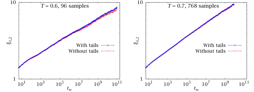
Figure 10.6: Left: Result of computing $\xi_{1,2}(t_{\mathrm{w}})$ in two different ways for our $96$ samples at $T=0.6$. In the red curve we stop the integration at the cutoff point where the relative error in $C_{4}(r,t_{\mathrm{w}})$ is greater than $1/3$. In the blue curve we add the contribution of the tail from that point on, estimated with an extrapolation using a fit to (10.14). The difference is small, but the second method maintains the power law behaviour until longer times. Right: Analogous plot for our $768$ samples at $T=0.7$. Now the effect is much less noticeable, since the increase in statistics has shifted the cutoff point.

This is the scaling function (10.14), using $a=0.4$. The fit is computed for $3\leq r\leq\min\{15,r_{\text{cutoff}}\}$, where the signal is still good. This correction turns out to be only relevant for the largest times and this only for our simulations with $\sim 100$ samples. For $T=0.7$, where we have $768$ samples, the cutoff distance is increased and the effect of the tail correction is hardly noticeable (Figure 10.6).

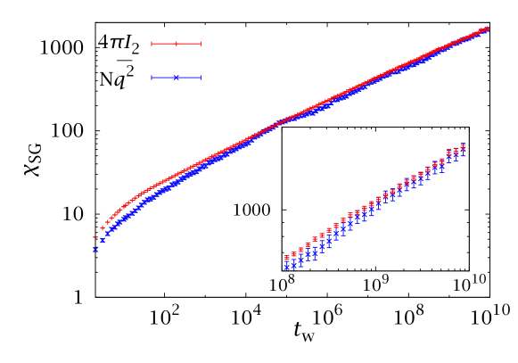
Figure 10.7: Computation of the spin-glass susceptibility for our $768$ samples at $T=0.7$ using both its straightforward definition (10.5) and the integral $I_{2}(t_{\mathrm{w}})$ of (10.22). $\chi_{\text{SG}}(t_{\mathrm{w}})=N\overline{q^{2}(t_{\mathrm{w}})}=4\uppi I_{2}(t_{\mathrm{w}})$. The second determination has been carried out using a self-consistent cutoff, which noticeably increases the precision. The inset details the upper-right corner of long times.

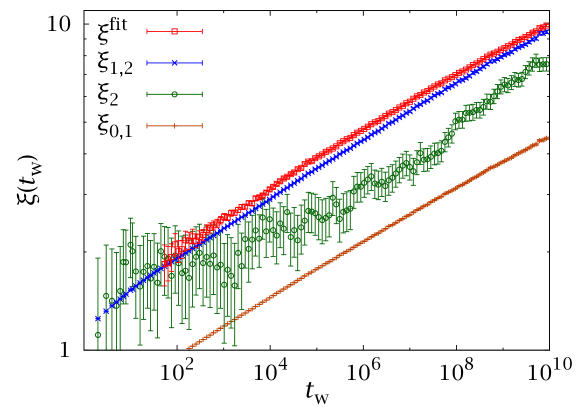
Figure 10.8: Comparison of several methods to estimate the coherence length $\xi(t_{\mathrm{w}})$ for our $768$ samples at $T=0.7$. We include the integral estimators $\xi_{1,2}$ and $\xi_{0,1}$ of (10.25), the second-moment estimate $\xi_{2}$ of (10.20) and the result of a fit to (10.13) using (10.14) and $a=0.4$. All curves are parallel for large $t_{\mathrm{w}}$, but the integral estimators are much more precise.

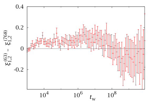
Figure 10.9: Difference between the coherence length $\xi_{1,2}(t_{\mathrm{w}})$ computed with the 63 samples of [janus:08b] and with the 768 of [janus:09b] (the errors are the quadratic sum of those for each simulation). The curves are compatible in the whole time range. Mind the dramatic statistical correlation in the sign of this difference.

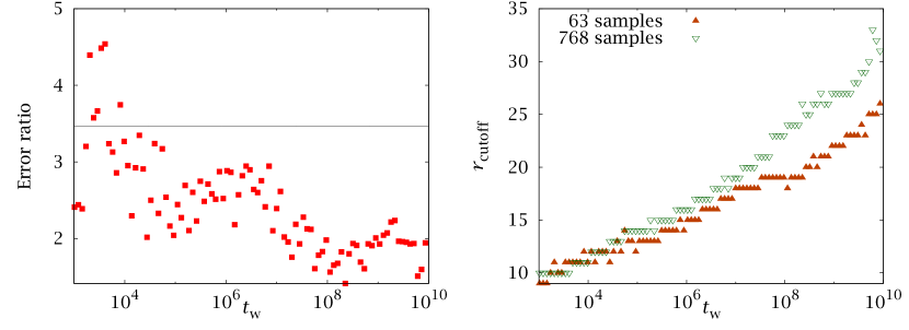
Figure 10.10: Left: Ratio of the errors in $\xi_{1,2}(t_{\mathrm{w}})$ for the simulations at $T=0.7$ with the $63$ samples of [janus:08b] and those of the $768$ samples of [janus:09b] (see text for discussion). The horizontal line is $\sqrt{768/63}\approx 3.46$. Right: Cutoff of the $I_{k}$ integrals as a function of time for both simulations.

We have claimed that this method yields a considerable increase in precision with respect to the computation of $\xi_{2}(t_{\mathrm{w}})$, or with the evaluation of $\xi$ from a fit. We offer two demonstrations of this. First, in Figure 10.7 we compare $4\uppi I_{2}(t_{\mathrm{w}})$ with $N\overline{q^{2}(t_{\mathrm{w}})}$, two quantities that should coincide (assuming rotational invariance). As we can see, the former is much more precise for the whole span of our simulation. As a second check, we have plotted in Figure 10.8 the coherence length for $T=0.7$ (where we have the best statistics) for several methods. All determinations are proportional, but the integral estimators are much more precise.

As a final test, we check not only our determination of $\xi$, but also its error estimate by comparing our $63$-sample computation of [janus:08b] with the improved 768-sample one of [janus:09b] for $T=0.7$. Figure 10.9 shows the difference in both determinations (the error in the difference is the quadratic sum of the individual errors, since both sets of samples are disjoint). We have excellent agreement for the whole time range. Notice that the points in this curve are correlated in time, so the fluctuations of neighbouring points are not independent.

Finally, we consider the error estimates in Figure 10.10. The expected error reduction is $\sqrt{768/63}\approx 3.5$, but we do not reach this value for most of our times. Notice that the relative statistical error in our error estimate is $\sim 1/\sqrt{2{\mathcal{N}}_{\text{samples}}}$, so the effect is not a fluctuation. The explanation is that the cutoff distance has increased for the simulation with $768$ samples, which trades statistical error for a reduction of systematic biases.

10.3.4 The isotropy of $C_{4}(r,t_{\mathrm{w}})$

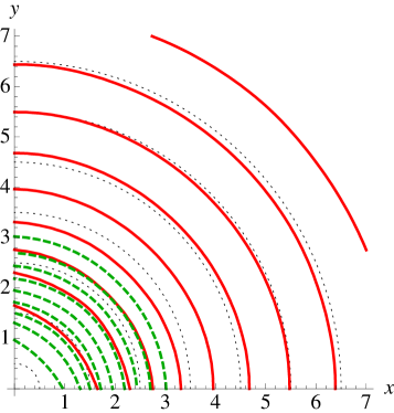
Figure 10.11: Level curves $C_{4}(\boldsymbol{r},t_{\mathrm{w}})=c$ for $c=0.3$ (dashed lines) and $c=0.1$ (solid lines) at $T=0.6$ (dotted lines are circles, for visual reference). The plot is restricted to the $z=0$ plane, for clarity. The innermost curve corresponds in both cases to $t_{\mathrm{w}}=4$ and the succeeding ones correspond to geometrically growing times ($t_{\mathrm{w}}=4\times 16^{i}$). As we can see, the deviations from isotropy are mainly due to lattice discretisation (i.e., functions of $r$). The errors are smaller than the thickness of the lines.

Throughout this section we have glossed over the issue of rotational invariance, assuming it is a good approximation. At all times we worked with correlations $C_{4}(r,t_{\mathrm{w}})$ restricted to the directions along the axes, hence ignoring most of the $N$ points for a given $t_{\mathrm{w}}$. The main motivation for this approach has traditionally been to avoid the computation of the whole $C_{4}(\boldsymbol{r},t_{\mathrm{w}})$, a task of $\mathcal{O}(N^{2})$ in a naive implementation. However, as detailed in Appendix A, we can turn the evaluation of an autocorrelation into the computation of two real Fourier transforms (the Wiener-Khinchin theorem). This latter task is $\mathcal{O}(N\log N)$ with the FFT algorithm. Therefore, computing the whole $C_{4}(\boldsymbol{r},t_{\mathrm{w}})$ implies no increase in numerical effort.

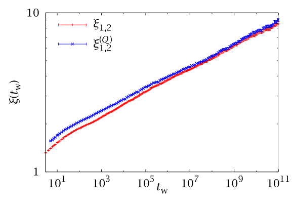
Figure 10.12: The coherence length computed with the whole correlation functions, $\xi^{(Q)}_{1,2}$, and with correlations along the axes, $\xi_{1,2}$. Both estimates coincide for large times and their errors are similar for the whole range. Data for $T=0.6$.

We examine in this section whether this complete correlation function is isotropic and whether we can take advantage of all the $N$ point to reduce statistical errors in the determination of $\xi(t_{\mathrm{w}})$. The first question is answered in Figure 10.11, where we plot level curves $C_{4}(\boldsymbol{r},t_{\mathrm{w}})=c$ for several values of $c$ and $t_{\mathrm{w}}$. As we can see, isotropy is recovered at quite small distances (remember we are only interested in $\xi\gtrsim 3$).

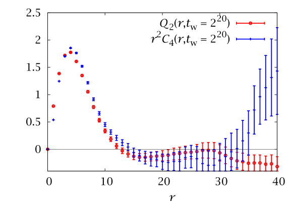
Figure 10.13: We compare the axes correlation $r^{2}C_{4}(r,t_{\mathrm{w}})$ with the shell-averaged correlation $Q_{2}(r,t_{\mathrm{w}})$. Both functions have similar precision for small distances, but the second is better behaved in the tails.

We next consider the possible improvement of our determination of $\xi(t_{\mathrm{w}})$ with the three-dimensional correlation function. In order to use our integral method we must first average over spherical shells,

$$Q_{k}(n,t_{\mathrm{w}})=\frac{\sum_{|\boldsymbol{r}|\in[n,n+1)}|\boldsymbol{r}|^{k}C_{4}(\boldsymbol{r},t_{\mathrm{w}})}{\sum_{|\boldsymbol{r}|\in[n,n+1)}1}\,.$$ (10.33)

Notice that $Q_{k}(0,t_{\mathrm{w}})=r^{k}C_{4}(0,t_{\mathrm{w}})=\delta_{k0}$. We can use $Q_{k}(m,t_{\mathrm{w}})$ as we did $r^{k}C_{4}(r,t_{\mathrm{w}})$ in our integral estimators. We would expect the resulting coherence length $\xi^{(Q)}_{1,2}(t_{\mathrm{w}})$ to coincide with $\xi_{1,2}(t_{\mathrm{w}})$ for large $t_{\mathrm{w}}$. However, if the fluctuations of $C_{4}(\boldsymbol{r},t_{\mathrm{w}})$ are independent, $\xi^{(Q)}_{1,2}$ will have smaller errors, due to the increase in statistics. In fact, see Figure 10.12, the statistical correlation between different parts of the lattice is so great that it renders the gain in precision negligible.

In short, the usual approximation of considering only correlation along the axes introduces neither a bias nor an increase in statistical errors. Still, the computation of $C_{4}(\boldsymbol{r},t_{\mathrm{w}})$ could be rewarding if one needed to consider $I_{k}$ with $k>2$ (Figure 10.13).

10.4  The thermoremanent magnetisation

$T$	$t_{\mathrm{w}}$	$c(t_{\mathrm{w}})$	$A_{0}(t_{\mathrm{w}})\times 10^{3}$	$\chi^{2}_{\text{d}}$/d.o.f.	$d(t_{\mathrm{w}})$
$0.6\approx 0.55T_{\mathrm{c}}$	2	$-0.1525(23)$	2.6(6)	14.7/64	$2.14(5)$
	4	$-0.1495(22)$	2.8(8)	15.5/64	$2.10(5)$
	8	$-0.1459(20)$	2.5(10)	17.4/64	$2.05(4)$
	16	$-0.1430(19)$	2.4(12)	17.5/64	$2.01(4)$
$0.7\approx 0.64T_{\mathrm{c}}$	2	$-0.1787(14)$	1.47(25)	23.3/50	$2.067(27)$
	4	$-0.1765(13)$	1.8(3)	18.4/50	$2.041(26)$
	8	$-0.1733(12)$	1.7(4)	18.9/50	$2.004(25)$
	16	$-0.1704(12)$	1.6(5)	15.4/50	$1.971(25)$
$0.8\approx 0.73T_{\mathrm{c}}$	2	$-0.210(8)$	1.7(10)	13.9/32	$1.98(9)$
	4	$-0.212(7)$	2.8(12)	11.1/32	$2.00(8)$
	8	$-0.208(7)$	3.0(14)	10.8/32	$1.96(8)$
	16	$-0.205(6)$	3.0(18)	8.43/32	$1.93(7)$

Table 10.2: Result of fitting the thermoremanent magnetisation to (10.34), for our three subcritical temperatures. We give the temperatures in terms of $T_{\mathrm{c}}$, to facilitate comparison with the experimental results of (10.35). For each fit we give the two parameters and the diagonal chi-square per d.o.f. The last column shows the result of computing $d=-cz$, in order to consider the scaling of equation (10.37). The fits are computed for $10^{6}<t<t_{\mathrm{w}}^{\mathrm{max}}(T)$ (cf. Table 10.1), which accounts for the different number of d.o.f. at each temperature.

The thermoremanent magnetisation of a spin glass is one of the easiest quantities to study experimentally. Indeed, it has been known since the 1980s that it decays with a power law (see [granberg:87, prejean:88] and references therein), even for temperatures very close to the critical point.

As we explained in Section 10.1.1, the two-time correlation $C(t,t_{\mathrm{w}})$ can be identified with the thermoremanent magnetisation (we have to choose $t_{\mathrm{w}}\sim 1$ as our initial ‘magnetised’ configuration and consider its overlap with the configuration at time $t\gg t_{\mathrm{w}}$). Following [parisi:97] we have fitted our data to the decay law

$$C(t,t_{\mathrm{w}})=A_{0}(t_{\mathrm{w}})+A_{1}(t_{\mathrm{w}})t^{c(t_{\mathrm{w}})}.$$ (10.34)

Notice that for a finite number of samples the correlation function does not actually go to zero for long times, hence the need for the finite asymptote $A_{0}(t_{\mathrm{w}})$. This is actually also a problem for experimental studies [granberg:87].

Table 10.2 shows the results of fits to (10.34) for our subcritical temperatures. The fits where computed in the range $10^{6}\leq t\leq t_{\mathrm{w}}^{\mathrm{max}}$, where $t_{\mathrm{w}}^{\text{max}}$ was given in Table 10.1. The lower bound of the fitting region can be varied along several orders of magnitude with no effect. Notice that the values of $\chi^{2}_{\text{d}}/\text{d.o.f.}$ are always much smaller than one, due to the correlations.

The asymptote $A_{0}(t_{\mathrm{w}})$ is in all cases of about $10^{-3}$, small compared to the the smallest value of $C(t,t_{\mathrm{w}})$ that we reach for our finite $t$, of about $10^{-2}$. The decay exponent is very small, $T$-dependent and exhibits a slight, but systematic dependence on $t_{\mathrm{w}}$ (a tendency that was already observed in [kisker:96]).

The experimental values for $c$ are, from [granberg:87],

$$c(0.55T_{\mathrm{c}}) \approx-0.12, c(0.67T_{\mathrm{c}}) \approx-0.14, c(0.75T_{\mathrm{c}}) \approx-0.17,$$ (10.35)

These values are slightly higher than our results of Table 10.2. The reason may be that our values of $c$ have been computed in fits where $t$ and $t_{\mathrm{w}}$ differ by as many as $10$ orders of magnitude, while in experimental work $t/t_{\mathrm{w}}\lesssim 10^{4}$.

We can recall here our study of full aging in Section 10.2, where we considered a fit in a narrower window of $t_{\mathrm{w}}\leq t\leq 10t_{\mathrm{w}}$. We can extrapolate our $\alpha(t_{\mathrm{w}})$ to an experimental time of $100$ s with a quadratic fit, such as we showed in Figure b.2. We thus obtain

$$-1/\alpha(t_{\mathrm{w}}=100\text{ s}) \approx-0.11, T=0.6\approx 0.55T_{\mathrm{c}},$$ (10.36a)

$$-1/\alpha(t_{\mathrm{w}}=100\text{ s}) \approx-0.12, T=0.7\approx 0.64T_{\mathrm{c}},$$ (10.36b)

$$-1/\alpha(t_{\mathrm{w}}=100\text{ s}) \approx-0.14, T=0.8\approx 0.73T_{\mathrm{c}}.$$ (10.36c)

These values still do not match the experimental values of (10.35). However, the difference between both sets seems to be roughly independent of temperature (this is best seen by plotting the parabolas defined by each of the sets of exponents). We believe this is due to an extrapolation error, with a similar bias for all temperatures.

$T$	$t_{\mathrm{w}}$	$t_{\text{min}}$	$e(t_{\mathrm{w}})$	$f(t_{\mathrm{w}})$	$\chi^{2}$/d.o.f.
$0.6$	$2$	$10^{3}$	$-0.236(7)$	$0.873(9)$	52.2/104
		$10^{6}$	$-0.30(6)$	$0.82(5)$	13.9/64
	$4$	$10^{3}$	$-0.203(6)$	$0.909(8)$	47.9/104
		$10^{6}$	$-0.25(4)$	$0.85(4)$	13.5/64
	$8$	$10^{3}$	$-0.176(4)$	$0.943(7)$	41.5/104
		$10^{6}$	$-0.21(3)$	$0.90(4)$	13.9/64
	$16$	$10^{3}$	$-0.158(4)$	$0.968(7)$	38.1/104
		$10^{6}$	$-0.19(3)$	$0.92(4)$	15.3/64
$0.7$	$2$	$10^{3}$	$-0.263(4)$	$0.890(4)$	43.0/90
		$10^{6}$	$-0.32(3)$	$0.84(3)$	14.4/50
	$4$	$10^{3}$	$-0.230(3)$	$0.921(4)$	71.9/90
		$10^{6}$	$-0.29(3)$	$0.862(25)$	12.8/50
	$8$	$10^{3}$	$-0.2003(23)$	$0.955(3)$	94.1/90
		$10^{6}$	$-0.253(23)$	$0.895(23)$	13.0/50
	$16$	$10^{3}$	$-0.1768(20)$	$0.985(3)$	138/90
		$10^{6}$	$-0.226(19)$	$0.921(22)$	10.6/50
$0.8$	$2$	$10^{3}$	$-0.302(16)$	$0.891(16)$	45.1/72
		$10^{6}$	$-0.5(3)$	$0.77(15)$	14.3/32
	$4$	$10^{3}$	$-0.257(12)$	$0.934(14)$	63.6/72
		$10^{6}$	$-0.6(4)$	$0.71(17)$	11.4/32
	$8$	$10^{3}$	$-0.223(10)$	$0.970(13)$	69.8/72
		$10^{6}$	$-0.49(24)$	$0.76(12)$	11.1/32
	$16$	$10^{3}$	$-0.192(8)$	$1.008(12)$	65.9/72
		$10^{6}$	$-0.40(19)$	$0.81(12)$	8.49/32

Table 10.3: Parameters of a fit to Eq. (10.39), offering an alternative description of the thermoremanent magnetisation. For each temperature, we present fits in the range $t_{\text{min}}\leq t\leq t_{\mathrm{w}}^{\text{max}}(T)$, where $t_{\text{min}}=10^{3},10^{6}$ and $t_{\mathrm{w}}^{\text{max}}(T)$ is given in Table 10.1.

Recall now that the coherence length $\xi(t_{\mathrm{w}})$ was also well represented by a power law. It follows that $C(t,t_{\mathrm{w}})$ should be a power of $\xi(t+t_{\mathrm{w}})$, at least for the small $t_{\mathrm{w}}$ of Table 10.2. In particular we write

$$C(t,t_{\mathrm{w}})\sim\bigl{[}\xi_{1,2}(t+t_{\mathrm{w}})\bigr{]}^{-d}.$$ (10.37)

We could perform a fit to (10.37) to find $d$, but we would have to contend with errors in both the $x$ and $y$ coordinates (see Section B.3.2). Rather, we combine equations (10.26) and (10.34) to find

$$d=cz.$$ (10.38)

Since both for $C(t,t_{\mathrm{w}})$ and for $\xi_{1,2}(t_{\mathrm{w}})$ we are computing one fit for each jackknife block, we can apply this relation block by block to obtain $d$ and its error estimate, without fitting for it directly. The result can be seen in Table 10.2. We obtain $d\approx 2$, with a temperature dependence at the limit of significance.

This is a potentially useful observation for experimental work since, as we said before, the thermoremanent magnetisation is relatively easy to measure (compared with the coherence length, in any case [joh:99]). Therefore, Eq. (10.37) could potentially be used as a definition of $\xi(t_{\mathrm{w}})$ for experimental work.

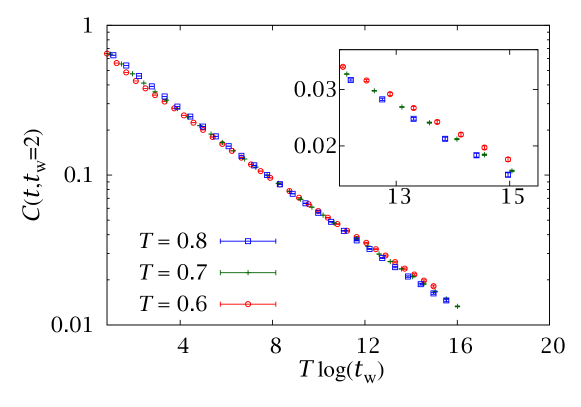
Figure 10.14: Coherence length $\xi_{1,2}(t_{\mathrm{w}})$ as a function of $T\log t_{\mathrm{w}}$, for three subcritical temperatures. Even if the three curves are not equal within errors, the overall scaling is suggestive.

As we have seen, there are several systematic effects in our results, mainly the incompatibility of (10.35) and (10.36) and the need for a finite asymptote $A_{0}(t_{\mathrm{w}})$ in (10.34). This suggests that (10.34) is perhaps not the best parameterisation. We can consider the alternative description

$$C(t,t_{\mathrm{w}})=B(t_{\mathrm{w}})\exp\bigl{[}e(t_{\mathrm{w}})(\log t)^{f(t_{\mathrm{w}})}\bigr{]}.$$ (10.39)

This would reproduce a power law if $f(t_{\mathrm{w}})=1$. Notice the difference of this functional form with a stretched exponential, discarded in [granberg:87] for our temperature range. The results of fits to (10.39) for several $t_{\mathrm{w}}$ and fitting ranges can be seen in Table 10.3. We observe that the fit parameters are very stable to variations in the fitting window. The value of $f(t_{\mathrm{w}})$ is incompatible with $1$, at least for $T=0.6,0.7$. However, from the point of view of the $\chi^{2}_{\text{d}}/\text{d.o.f.}$, both (10.34) and (10.39) are equally good.

Finally, let us go back to (10.34) and Table 10.2. We see that the exponent $c(t_{\mathrm{w}})$ is roughly linear in $T$. This suggests that the thermoremanent magnetisation could be a temperature-independent function of $T\log(t)$. We have tested this conjecture in Figure 10.14 and found it to be only approximate.

10.5  Dynamical heterogeneities

Thus far, we have characterised the spin-glass dynamics globally through the two-time correlation function. We have found this dynamics to be extremely slow and we have used a growing coherence length to monitor the evolution.

However, the dynamics is actually heterogeneous across the system, with local regions behaving differently from the bulk. As we said in Section 9.1.3, the study of these dynamical heterogeneities is a potential point of contact between studies of spin glasses and of general glassy behaviour.

The traditional numerical approach to dynamic heterogeneities has been the computation of coarse-grained correlation functions. These are defined as an average over a cell of size $\ell^{D}$, with $\ell\ll L$. The characteristic length scale for dynamical heterogeneities can then be assessed through the probability distribution of these coarse-grained correlations. For $\ell$ much larger than the correlation length, one would expect the fluctuations to be averaged out, and the resulting coarse-grained correlation would resemble the global one. For small $\ell$, however, strong deviations from a Gaussian behaviour are present [jaubert:07]. One defines, then, the correlation length as the crossover length.

Here we follow a different approach, consisting in the study of the two-time spatial correlation $C_{2+2}(\boldsymbol{r},t,t_{\mathrm{w}})$ of Eq. (10.16). This observable was introduced in [jaubert:07], but the time scales accessible to that work did not permit the measurement of correlation lengths greater than a couple of lattice spacings.

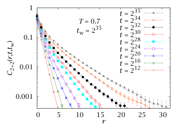
Figure 10.15: The two-time spatial correlation function $C_{2+2}(r,t,t_{\mathrm{w}})$ defined in (10.16) as a function of $r$, for several values of $t$. We consider a long waiting time of $t_{\mathrm{w}}=2^{35}$, for our $63$-sample simulations at $T=0.7$.

We have plotted the correlation length $C_{2+2}(r,t,t_{\mathrm{w}})$ (we use the same convention for axially oriented correlations as for $C_{4}$) in Figure 10.15, for a large waiting time. From this plot we can see, qualitatively, that the correlation reaches several lattice spacings for large times.

Recalling the one-to-one nature of $C(t,t_{\mathrm{w}})$ as a function of $t$ for fixed $t_{\mathrm{w}}$, we eliminate $t$ as independent variable in favour of $C^{2}$, using a cubic spline as our interpolating method. We consider, then, a correlation length $\zeta(C^{2},t_{\mathrm{w}})$ from the long-distance behaviour of $C_{2+2}(r,t(t_{\mathrm{w}},C^{2}),t_{\mathrm{w}})$, in complete analogy with the case of $\xi(t_{\mathrm{w}})$ and $C_{4}(r,t_{\mathrm{w}})$, recall Eq. (10.17). This correlation length is computed with the methods of Section 10.3.1.

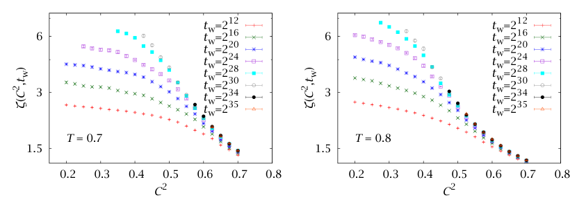
Figure 10.16: Correlation length $\zeta(C^{2},t_{\mathrm{w}})$ as a function of $C^{2}$ for several waiting times. We plot our results for $T=0.7$ with $63$ samples and for $T=0.8$ ($96$ samples).

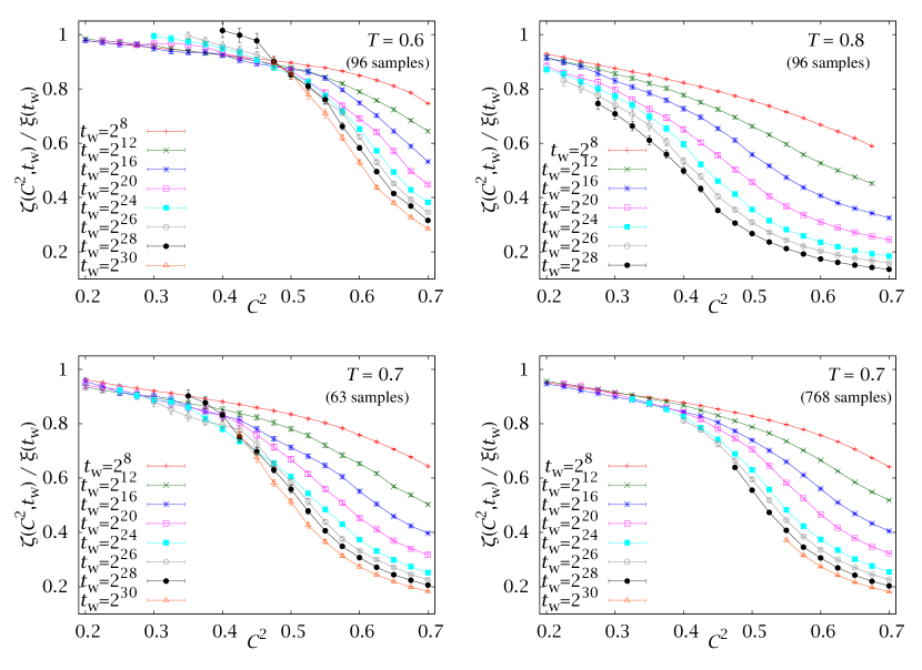
Figure 10.17: Behaviour of the ratio $\zeta_{1,2}(C^{2},t_{\mathrm{w}})/\xi_{1,2}(t_{\mathrm{w}})$ as a function of $C^{2}$ for several values of $t_{\mathrm{w}}$. We observe a crossover behaviour from a finite limit at small $C^{2}$ to a vanishing limit for large $C^{2}$. Notice that for $T=0.7$ we plot both our set with $63$ longer samples and our set with $768$ shorter ones.

We have plotted $\zeta(C^{2},t_{\mathrm{w}})$ as a function of $C^{2}$ for several $t_{\mathrm{w}}$ at $T=0.7,0.8$ in Figure 10.16. We observe that the evolution in $t_{\mathrm{w}}$ distinguishes two regimes. For large $C^{2}$ the correlation length approaches a $t_{\mathrm{w}}$-independent enveloping curve. This corresponds with the low-$t$ regime, which quickly approaches the translationally invariant sector of the dynamics. When $C^{2}$ drops below $q_{\text{EA}}^{2}$, however, we are in an aging regime, where the correlation length diverges in the large-$t_{\mathrm{w}}$ limit.

Since one would expect the divergence in the aging limit to behave as $\xi(t_{\mathrm{w}})$, it is useful to consider the scaling variable

$$R(C^{2},t_{\mathrm{w}})=\frac{\zeta(C^{2},t_{\mathrm{w}})}{\xi(t_{\mathrm{w}})}\,.$$ (10.40)

We expect

$$\lim_{t_{\mathrm{w}}\to\infty}R(C^{2}<q_{\text{EA}}^{2}) >0.$$ (10.41)

$$\lim_{t_{\mathrm{w}}\to\infty}R(C^{2}>q_{\text{EA}}^{2}) =0.$$ (10.42)

We show this quantity for our three subcritical temperatures in Figure 10.17. For $T=0.7$ we show both our longer simulations with $63$ samples and our more precise set with $768$.

Clearly, there is a crossover, which is best observed for $T=0.6$. However, we face a dilemma: for low $T$ the growth of the coherence length is very slow and we do not see the large-$C^{2}$ behaviour as clearly, while for high $T$ the value of $q_{\text{EA}}$ is too low for us to appreciate the crossover at low $C^{2}$ (notice that the spin glass undergoes a second-order transition, so $q_{\text{EA}}(T_{\text{c}})=0$).

$T$	$C^{2}$	$z_{\zeta}$	$\chi^{2}_{\zeta}$/d.o.f.	$z$
$0.6$	$0.200$	$13.4(6)\ \ \ \$	$0.01/2$	$14.06(25)$
$0.7$	$0.200$	$11.14(20)$	$0.69/3$	$11.56(13)$
$0.8$	$0.100$	$9.56(17)$	$3.73/5$	$\ \ 9.42(15)$

Table 10.4: Value of the dynamic exponent $z_{\zeta}$ of Eq. (10.43) for three subcritical temperatures. We also give our best determination of the dynamic critical exponent $z$ from Table 10.1.

In short, while our data include long enough times to appreciate the behaviour qualitatively, they are not sufficiently clean for us to characterise the scaling behaviour at the crossover point. In Section 10.8 we shall take on this problem again with equilibrium methods. We shall show how the crossover in the behaviour of dynamical heterogeneities can be interpreted as a proper phase transition and how its critical parameters, computed in equilibrium, can be used to characterise the dynamics.

For now we address the simpler problem of the scaling of $\zeta(C^{2},t_{\mathrm{w}})$ in the low-$C^{2}$ sector. Since in this situation $\zeta$ and $\xi$ differ only in a constant factor close to one, we consider the following ansatz

$$\zeta(C^{2}<q_{\text{EA}}^{2},t_{\mathrm{w}})=A_{\zeta}t_{\mathrm{w}}^{1/z_{\zeta}},$$ (10.43)

where $z_{\zeta}$ is expected to be similar to $z$. For each $T$, we have performed fits to (10.43) for a value of $C^{2}$ expected to be below $q_{\text{EA}}$. We note that the value of $q_{\text{EA}}$ has consistently been overestimated in the literature, as we shall show in the following sections. In fact, in order to be safe we have simply fitted the lowest value of $C^{2}$ for which we could obtain an acceptable number of degrees of freedom in the fits.

The results are shown in Table 10.4, where we can see that $z_{\zeta}(T)$ is indeed similar to $z(T)$, although we can measure it with much worse precision.

10.6  The translationally invariant sector

In Section 10.2 we left pending the question of computing the stationary part of the temporal correlation function. As we noted there, a naive extrapolation is complicated, because we have to consider the limit $t_{\mathrm{w}}\to\infty$, which is also strongly $t$-dependent.

Here we address this problem, taking advantage of the characteristic lengths we have computed. In particular, we study the following dynamical variable

$$x(t,t_{\mathrm{w}})=\left(\frac{\zeta(t,t_{\mathrm{w}})}{\xi(t_{\mathrm{w}})}\right)^{2}\,.$$ (10.44)

Following the discussion of the previous section, the translationally invariant sector is recovered in the limit $x\to 0$ (where $x$ is essentially $\xi^{-2}(t_{\mathrm{w}})$ in its natural units for each $t$). However, this limit is much easier to compute in a controlled way than $t_{\mathrm{w}}\to\infty$.

Figure 10.18: The temporal correlation function as a function of $x(t,t_{\mathrm{w}})$, Eq. (10.44), with an inset showing a close-up of the small-$x$ limit (equivalent to an extrapolation to $t_{\mathrm{w}}\to\infty$). Plot for our $768$-sample simulation at $T=0.7$.

We have plotted $C(t,t_{\mathrm{w}})$ against $x(t,t_{\mathrm{w}})$ for our simulations at $T=0.7$ in Figure 10.18. We see that, indeed, the curve is very smooth in the small-$x$ limit, and an extrapolation seems feasible (see Inset). Furthermore, the curves for different $t$ become parallel as $t$ grows, which suggests the existence of a smooth scaling function $C(t,t_{\mathrm{w}})=C_{\infty}(t)+f(x)$. In particular, we consider the following functional form

$$C(t,x)=C_{\infty}(t)+a_{1}(t)x+a_{2}(t)x^{2}.$$ (10.45)

However, a naive extrapolation using (10.45) is still problematic. The reason is that we have errors both for $C$ and for $x$ (i.e., for both the $x$ and $y$ coordinates in the fit). Luckily, however, the errors were similar in both directions and for all points. Therefore, we can use the method explained in Section B.3.2. We compute the fits for $x\leq 0.5$, using $\xi_{1,2}$ and $\zeta_{1,2}$ as our estimates of the characteristic lengths.

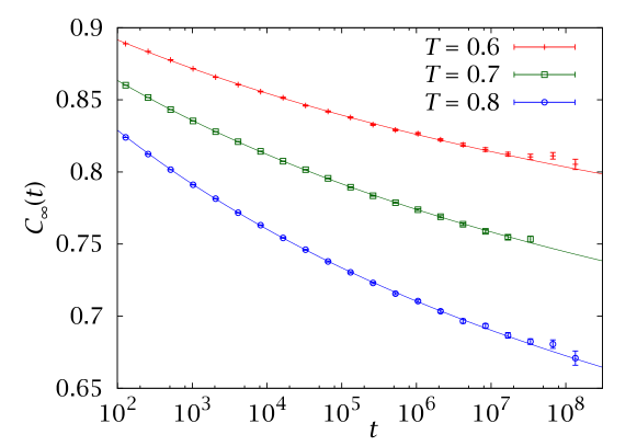
Figure 10.19: Stationary part $C_{\infty}(t)$ of the two-time correlation function $C(t,t_{\mathrm{w}})$ for $T=0.7,0.7,0.8$, obtained from the extrapolations in Figure 10.18.

This method has allowed us to compute $C_{\infty}(t)$ with remarkable accuracy for $t\lesssim 10^{8}$ (Figure 10.19). Now that we have this function, we could try a second extrapolation to find $q_{\text{EA}}$,

$$\lim_{t\to\infty}C_{\infty}(t)=q_{\text{EA}}.$$ (10.46)

However, this second extrapolation turns out to be very difficult, because now we cannot avoid the issue of considering the infinite limit explicitly. Furthermore, we lack a convincing theoretical expectation as to the functional form of $C_{\infty}(t)$.

The simplest option is a power law decay,

$$C_{\infty}(t)=q_{\text{EA}}+At^{-B}.$$ (10.47)

This equation yielded very good fits for $T=0.6,0.8$ (Table 10.5, but the values of the exponents were very small, $B\sim 0.05$. The smallness of $B$ makes the extrapolation extremely risky, since it means that $q_{\text{EA}}$ is going to be much smaller than our range of values for $C_{\infty}(t)$. We note that this slow evolution has led some authors to overestimate $q_{\text{EA}}$ in the past (with larger errors, $C_{\infty}$ seems almost constant).

$T$	Fitting range	Logarithm		Power law
		$q_{\text{EA}}$	$\chi^{2}_{\text{d}}/\text{d.o.f}$	$q_{\text{EA}}$	$B\times 10^{2}$	$\chi^{2}_{\text{d}}/\text{d.o.f}$
$0.6$	$[10^{2},10^{8}]$	0.607(16)	34.1/17	0.730(8)	5.7(4)	31.2/17
	$[10^{3},10^{8}]$	0.62(3)	7.23/14	0.733(14)	5.8(7)	7.59/14
	$[10^{4},10^{8}]$	0.62(5)	6.25/10	0.726(24)	5.4(12)	6.32/10
$0.7$	$[10^{2},10^{8}]$	0.497(10)	23.7/17	0.656(5)	6.16(18)	32.6/17
	$[10^{3},10^{8}]$	0.474(21)	18.9/14	0.637(11)	5.5(3)	18.5/14
	$[10^{4},10^{8}]$	0.49(5)	15.0/10	0.63(3)	5.4(9)	15.3/10
$0.8$	$[10^{2},10^{8}]$	0.371(13)	6.50/17	0.568(7)	6.56(20)	9.39/17
	$[10^{3},10^{8}]$	0.368(24)	5.53/14	0.556(12)	6.2(4)	4.27/14
	$[10^{4},10^{8}]$	0.40(6)	4.31/10	0.56(3)	6.4(11)	3.82/10

Table 10.5: Estimate of $q_{\text{EA}}$ for three subcritical temperatures, using two different extrapolating functions. For $T=0.6,0.8$ both are very good, but at $T=0.7$ (where we have better statistics) they are somewhat forced. This suggests that the real $q_{\text{EA}}$ probably lies in between our two estimates. For the power law extrapolation, Eq. (10.47), we also quote the exponent $B$. Notice that this exponent is not proportional to $T$. See Section 10.8 for a considerably more precise determination of this parameter.

Perhaps more disquieting, it may seem that a low enough value of $B$ would allow for the possibility that $q_{\text{EA}}=0$. In order to dispel this notion, we have tried a second fit to a logarithmic decay,

$$C_{\infty}(t)=q_{\text{EA}}+\frac{A}{B+\log t}\ .$$ (10.48)

We stress that this ansatz lacks theoretical basis, we merely take it as a lower bound on the value of $q_{\text{EA}}$. Numerically, it turns out, the logarithmic fit is as good as the exponential one for $T=0.6,0.8$, even if it produces incompatible values of $q_{\text{EA}}$ (Table 10.5).

Furthermore, if we try both fitting functions for our $T=0.7$ data, where we have much better statistics, we find that they were somewhat forced. This leads us to conclude that the real asymptotic behaviour of $C_{\infty}(t)$ is probably something in between (10.47) and (10.48). We can use the difference between both methods with a fitting window of $t\in[10^{3},10^{8}]$ as our uncertainty interval,

$$0.62 \leq q_{\text{EA}}(T=0.6)\leq 0.733,$$ (10.49a)

$$0.474 \leq q_{\text{EA}}(T=0.7)\leq 0.637,$$ (10.49b)

$$0.368 \leq q_{\text{EA}}(T=0.8)\leq 0.556.$$ (10.49c)

Even with our unprecedently long simulations, we are still at the threshold of being able to compute $q_{\text{EA}}$ with dynamical methods. In Section 10.8 we shall perform an equilibrium computation of this quantity.

10.7  Equilibrium analogues and the time-length dictionary

As we have seen, the non-equilibrium approach, while straightforward, is limited when one needs to perform some delicate analyses, such as the estimation of $q_{\text{EA}}$. Therefore, one should complement it with equilibrium computations. Recall that we are working in a framework where the equilibrium phase is unreachable for experimental systems, yet conditions the non-equilibrium dynamics. Remember, for instance, the relation between the fluctuation-dissipation ratio of Figure 9.4 and the equilibrium $p(q)$ [franz:98, franz:99].

In this section we take the qualitative statics-dynamics relation one step farther. Our proposal is that the equilibrium correlation functions computed for systems of finite size should reproduce their non-equilibrium counterparts in the thermodynamical limit for finite time. An infinite system with a finite coherence length $\xi(t_{\mathrm{w}})$ can, very roughly, be considered as a collection of systems of size $L\sim\xi(t_{\mathrm{w}})$ in equilibrium, with some reservations. This relation should establish a time-length dictionary $t_{\mathrm{w}}\leftrightarrow L$, which is our objective in this section.

In particular, we shall consider the equilibrium spatial autocorrelation,

$$C_{4}(\boldsymbol{r})=\frac{1}{N}\sum_{\boldsymbol{x}}\overline{\braket{q_{\boldsymbol{x}}q_{\boldsymbol{x}+\boldsymbol{r}}}}.$$ (10.50)

We want to relate $C_{4}(\boldsymbol{r})$ to $C_{2+2}(\boldsymbol{r},t,t_{\mathrm{w}})$. As we have said, the waiting time $t_{\mathrm{w}}$ can be related to $L$, but what of $t$? The answer lies in the, already exploited, one-to-one relation between $t$ and the two-time overlap $C(t,t_{\mathrm{w}})$ at fixed $t_{\mathrm{w}}$. In equilibrium, the dependence on $C$ is replaced by the computation of correlation functions conditioned to a fixed value of $q$. Finally, we note that (10.50) is non-connected, unlike $C_{2+2}$, as we defined it in (10.16). Therefore, we shall consider here a non-connected version of $C_{2+2}$,

$$C_{2+2}^{\prime}(\boldsymbol{r},t,t_{\mathrm{w}})=\overline{\frac{1}{N}\sum_{\boldsymbol{x}}c_{\boldsymbol{x}}(t,t_{\mathrm{w}})c_{{\boldsymbol{x}}+\boldsymbol{r}}(t,t_{\mathrm{w}})}\ .$$ (10.51)

Our objective, then, for this section, is finding a relation between

$$C_{2+2}^{\prime}\bigl{(}\boldsymbol{r},t(C(t,t_{\mathrm{w}})),t_{\mathrm{w}}\bigr{)}\longleftrightarrow C_{4}(\boldsymbol{r}|q).$$ (10.52)

We still have to provide a workable definition of the $q$-conditioned $C_{4}(\boldsymbol{r}|q)$. In order to do this, let us step back for a moment and consider the pdf of the spin overlap,

$$p_{1}(q)=\overline{\biggl{\langle}\delta\biggl{(}q-\frac{1}{N}\sum_{\boldsymbol{x}}q_{\boldsymbol{x}}\biggr{)}\biggr{\rangle}}.$$ (10.53)

This definition is completely analogous to the $p_{1}(m)$ of (4.8) we considered in Chapter 3. Like in that case, the $p_{1}(q)$ is not smooth for finite systems, but rather the sum of $N+1$ Dirac deltas. Even if we are not considering a tethered formalism here, we can borrow the cure to this problem. In particular, we define our smooth $p(q)$ as the convolution of $p_{1}(q)$ with a Gaussian of width $1/\sqrt{N}$

$$p(q=c) =\int_{-\infty}^{\infty}\mathrm{d}q^{\prime}\ p_{1}(q^{\prime})\mathcal{G}_{N}(c-q^{\prime})=\overline{\biggl{\langle}\mathcal{G}_{N}\biggl{(}c-\frac{1}{N}\sum_{\boldsymbol{x}}q_{\boldsymbol{x}}\biggr{)}\biggr{\rangle}},$$ (10.54)

$$\mathcal{G}_{N}(x) =\sqrt{\frac{N}{2\uppi}}\mathrm{e}^{-Nx^{2}/2}.$$ (10.55)

The pdf $p(q)$ is an interesting observable in its own right, since, as we saw in Chapter 9, its thermodynamical limit is very different in the droplet and RSB pictures. We shall study it in detail in Section 11.1.

Now, we can generalise our treatment of $p(q)$ to define conditional expectation values at fixed $q$

$$\mathrm{E}(O|q=c)=\frac{\overline{\biggl{\langle}O\mathcal{G}_{N}\biggl{(}c-\frac{1}{N}\sum_{\boldsymbol{x}}q_{\boldsymbol{x}}\biggr{)}\biggr{\rangle}}}{\overline{\biggl{\langle}\mathcal{G}_{N}\biggl{(}c-\frac{1}{N}\sum_{\boldsymbol{x}}q_{\boldsymbol{x}}\biggr{)}\biggr{\rangle}}}.$$ (10.56)

Of course, the standard expectation values can be recovered from the $\mathrm{E}(O|q)$,

$$\overline{\braket{O}}=\int_{-\infty}^{\infty}\mathrm{d}q\ p(q)\mathrm{E}(O|q).$$ (10.57)

Finally, we define the fixed-$q$ correlation function as

$$C_{4}(\boldsymbol{r}|q)=\mathrm{E}\left(\frac{1}{N}\sum_{\boldsymbol{x}}q_{\boldsymbol{x}}q_{{\boldsymbol{x}}+\boldsymbol{r}}\middle|q\right).$$ (10.58)

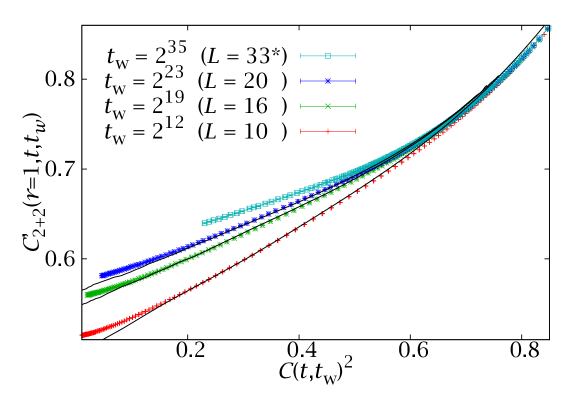
Figure 10.20: Plot of the off-equilibrium non-connected correlation $C_{2+2}^{\prime}(r=1,C^{2},t_{\mathrm{w}})$ of Eq. (10.51) for several waiting times at $T=0.7$. We compare it with the equilibrium $C_{4}(r=1|q)$, Eq. (10.58), using data from [contucci:07] (continuous lines), finding that they are accurately matched through the time-length dictionary $L\approx 3.7\xi(t_{\mathrm{w}})$. According to this, the correlation for $t_{\mathrm{w}}=2^{32}$ would correspond to an $L=33$ system.

In [janus:08b] we compared our non-equilibrium $C_{2+2}^{\prime}(r=1,t,t_{\mathrm{w}})$ with the equilibrium $C_{4}(r=1|q)$, using equilibrium data from [contucci:06, contucci:07], at $T=0.7$. The result is plotted in Figure 10.20. We can see, how, indeed, the equilibrium correlation functions reproduce the non-equilibrium ones through a consistent time-length correspondence. More precisely, the non-equilibrium correlations at time $t_{\mathrm{w}}$ can be matched to the equilibrium ones with the time-length dictionary

$$L(t_{\mathrm{w}})\approx 3.7\xi_{1,2}(t_{\mathrm{w}}).$$ (10.59)

In [janus:08b] we used this equivalence to predict that $t_{\mathrm{w}}=2^{32}$ would correspond to an $L=33$ system. We note that, due to our discretisation of measuring times, we have only established this dictionary up to the nearest power of $2$.

In the previous analysis, we were limited by the equilibrium data, which only reached $L=20$ and did not consider correlations for $r>1$. We afterwards ran our own equilibrium simulations with Janus, reaching $L=32$ and taking more thorough measurements (see Appendix E for details on these simulations and thermalisation checks). Our lowest temperature for our largest lattices was precisely $T=0.7$. We simulated $L=8,12,16,24,32$. We can now use this much more precise equilibrium simulation to improve on the conclusions of Figure 10.20.

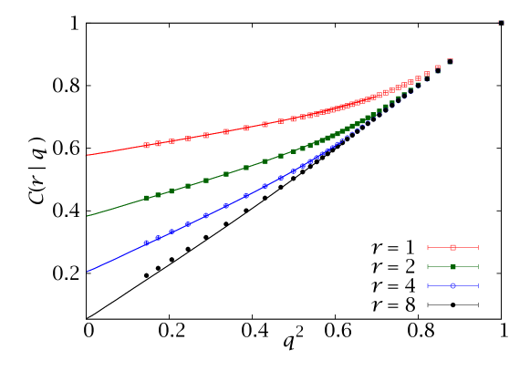
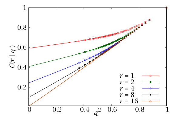
Figure 10.21: Comparison of our non-equilibrium correlation functions $C^{\prime}_{2+2}(r,C^{2},t_{\mathrm{w}})$ (points) and our equilibrium $C_{4}(r|q)$ (lines) at $T=0.7$. In the top panel we compare $L=24$ with $t_{\mathrm{w}}=2^{26}$ and on the bottom one we consider $L=32$ and $t_{\mathrm{w}}=2^{31}$. The errors in both data sets are comparable and smaller than the points.

According to the time-length dictionary, then, our $L=32$ simulations would correspond to $t_{\mathrm{w}}\approx 2^{31}$ and our $L=24$ ones would correspond to $t_{\mathrm{w}}\approx 2^{26}$. We have plotted both cases in Figure 10.21, this time for several values of $r$, corroborating our prediction of [janus:08b]. Notice that in a finite lattice $C_{4}(r|q)$ can only be computed up to $r=L/2$, while the non-equilibrium $C_{2+2}^{\prime}(r,t,t_{\mathrm{w}})$ is defined for arbitrary distance. However, we find a very good matching even for relatively large values of $r$.

10.7.1 The experimental length scale

As we can see, even relatively long times $2^{32}\text{ MCS}\sim 10^{10}\text{ MCS}\sim 0.01\text{ seconds}$, correspond to the equilibrium behaviour for quite small systems. This raises the question of the relevance of the thermodynamical limit for experimental physics. Indeed, for a typical experimental scale of $1$ hour, that is, for a $t_{\mathrm{w}}\approx 3.6\times 10^{15}\text{ MCS}$, we can extrapolate the expected coherence length with equation (10.26) and the data in Table 10.1. We conclude that

$$L(t_{\mathrm{w}})\approx 3.7\xi_{1,2}(t_{\mathrm{w}})\qquad\Longrightarrow\qquad 1\text{ hour}\longleftrightarrow L=110$$ (10.60)

That is, the equilibrium length scale relevant to the non-equilibrium experiments is not the thermodynamical limit, but rather $L\sim 100$.

This concept of experimental length scale will be extremely relevant in the next Chapter, where we try to elucidate the nature of the spin-glass phase. We shall find there that making extrapolations to $L\to\infty$ is very difficult, but that extrapolating to $L=110$ is safe.

As a final comment, we point out that some authors have proposed a modified scaling for the coherence length, substituting the power law with a more complex functional form [bouchaud:01]. This was studied in Section 6 of [janus:09b] and found to fit our non-equilibrium simulations (the underlying reason being that $1/z$ is very small and it is very difficult to distinguish a small power from a logarithm with numerical data). If this modified scaling were to hold instead of the power-law behaviour, the length scale equivalent to one hour would be smaller than $L=110$.

10.8  The phase transition in the dynamical heterogeneities

The previous section presented one of our most important results: the statics-dynamics equivalence can be made quantitative. We shall now take this observation one step further and use the equilibrium correlation functions to understand the crossover in the behaviour of the dynamical heterogeneities. Recall that, for large $C$, the two-time correlation length $\zeta(C,t_{\mathrm{w}})$ reached a $t_{\mathrm{w}}$-independent value, while for small $C$ it grew as the coherence length $\xi(t_{\mathrm{w}})$.

Our dynamical study was precise enough for us to observe this phenomenon, but not to study it quantitatively. One of the major limiting factors was that the crossover value, $q_{\text{EA}}$, was very low, so even with our long simulations we did not have enough statistics in the low-$C$ sector. However, one of the advantages of an equilibrium study is that we can cover the whole range of $q$. To this end we can consider the behaviour of the connected correlation function at fixed $q$. Below $q_{\text{EA}}$ (and for $T<T_{\text{c}}$), one expects

$$C_{4}(\boldsymbol{r}|q)-q^{2} =\frac{A_{q}}{r^{\theta(q)}}+\ldots, |q| <q_{\text{EA}}.$$ (10.61)

The droplet and RSB pictures have very different predictions for the structure exponent $$\theta(q) 0\leq\theta(q)<D$$, which we shall study in detail in Section 11.3. For the moment, we only need that , on which both theories agree. In order to study these connected correlations in position space, one has to perform a subtraction that complicates the analysis (Section 11.3 and cf. [contucci:09]). Instead, in this Section we work in Fourier space. The scaling behaviour is now

$$\hat{C}_{4}({\boldsymbol{k}}|q) \propto k^{\theta(q)-D}+\ldots, |q| <q_{\text{EA}}.$$ (10.63)

On the other hand [dedominicis:98, contucci:09],

$$\hat{C}_{4}({\boldsymbol{k}}|q) \propto\frac{1}{k^{2}+\xi_{q}^{-2}}, |q| >q_{\text{EA}}.$$ (10.64)

This equation defines a correlation length $\xi_{q}$ —cf. Eq. (5.6)— which diverges when $|q|\to q_{\text{EA}}$ from above.

In what follows we shall use the notation:

$$F_{q}^{(n)} =\hat{C}_{4}(n{\boldsymbol{k}}_{\text{min}}|q), F_{q} =F_{q}^{(1)}.$$ (10.65)

The two scalings (10.63) and (10.64) for $\hat{C}_{4}$ reproduce the crossover behaviour that we found when studying $\zeta(C,t_{\mathrm{w}})$: $F_{q}\sim L^{D-\theta(q)}$ for $|q|<q_{\text{EA}}$ but $F_{q}\sim 1$ for $|q|>q_{\text{EA}}$. In the large-$L$ limit, the crossover becomes a phase transition where

$$\xi_{q}^{(\infty)}\propto\frac{1}{(q-q_{\text{EA}})^{\hat{\nu}}}\ .$$ (10.66)

Here $\hat{\nu}$ is a critical exponent, in principle different from the thermal critical exponent at $T_{\mathrm{c}}$. This concept of a phase transition at $T<T_{\mathrm{c}}$ as we vary $q$ may seem unorthodox for spin glasses. However, a very similar picture appears in the study of the equation of state for Heisenberg ferromagnets [brezin:73].

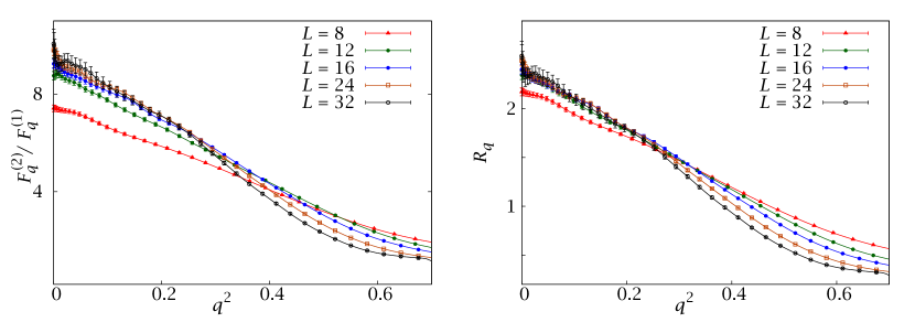
Figure 10.22: Left: Plot of the dimensionless quantity $F_{q}^{(1)}/F_{q}^{(2)}$. Right: Same plot, but now we add factors of $\sin^{2}(n\uppi/L)$ to avoid trivial free-field scaling corrections and plot $R_{q}=\bigl{[}F_{q}^{(1)}\sin(\uppi/L)\bigr{]}/\bigl{[}F_{q}^{(2)}\sin(2\uppi/L)\bigr{]}$. In both cases the curves merge below $q_{\text{EA}}$ (as in a Kosterlitz-Thouless transition), but we cannot distinguish the critical point with much precision.

We can study this phase transition using finite-size scaling, as we did for the Ising model and the DAFF. Up to scaling corrections, we have

$$F_{q}^{(n)}=L^{D-\theta(q_{\text{EA}})}G_{n}\bigl{(}L^{1/\hat{\nu}}(q-q_{\text{EA}})\bigr{)}.$$ (10.67)

Notice that this approach also has close parallels with the condensation transition, which can be studied with Ising ferromagnets. In what follows, just as in the previous section, we shall work at $T=0.703$.

As in previous chapters, we want to exploit (10.67) using phenomenological renormalisation. The first step in those analyses was finding some suitable dimensionless quantity and studying the intersections of its curves for different $L$. The only obvious such quantity that we have here is $F^{(n)}_{q}/F^{(m)}_{q}$. Unfortunately, these ratios do not show clear intersections. Indeed, in the case where $\theta(|q|<q_{\text{EA}})>0$ the whole phase $|q|<q_{\text{EA}}$ will be critical and we will be in a situation analogous to a Kosterlitz-Thouless transition [kosterlitz:73], where the curves merge, rather than intersect, at the critical point. Figure 10.22 suggests that this may be the case, but it is not possible to get a clear determination of $q_{\text{EA}}$ from these data.

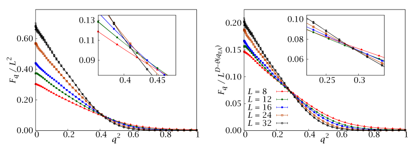
Figure 10.23: Plot of $F_{q}/L^{y}$ against $q^{2}$ for all our system sizes at $T=0.703$ and two values of $y$. In the left panel we consider the free-field scaling $F_{q}({\boldsymbol{k}})\propto k^{-2}$, that is, $y=2$. In the right panel we consider $y=2.35\approx D-\theta(q_{\text{EA}})$ (see below). The insets are closeups of the crossing region and both are shown at the same scale.

We have therefore adopted an alternative approach. Rather than looking for dimensionless quantities we consider the ratios $F_{q}/L^{y}$, where $y$ is a continuous parameter,

$$F_{q}/L^{y}=L^{\epsilon-y}G_{1}\bigl{(}L^{1/\hat{\nu}}(q-q_{\text{EA}})\bigr{)},\qquad\epsilon=D-\theta(q_{\text{EA}}).$$ (10.68)

Now, as long as $y<D-\theta(0)$, it follows that, in the large-$L$ limit, $F_{q}/L^{y}$ vanishes for $|q|>q_{\text{EA}}$ and diverges for $|q|<q_{\text{EA}}$. Therefore, the curves for these quantities as a function of $q$ for different $L$ will also intersect. We show two values of $y$ in Figure 10.23.

Now we can once again analyse these intersections with the quotients method. We consider pairs of lattices $(L,sL)$. Then, operating with (10.68) we see that the crossing points $q_{L,y}^{(s)}$ scale as

$$q_{L,y}^{(s)} =q_{\text{EA}}+A_{y}^{(s)}L^{1/\nu}+\ldots, A_{y}^{(s)} =\frac{G_{1}(0)}{G^{\prime}_{1}(0)}\frac{s^{\epsilon-y}-1}{s^{1/\nu}-s^{\epsilon-y}}\ ,$$ (10.69)

where the dots denote corrections to leading scaling. A fit to this equation could produce the values of $q_{\text{EA}}$ and of $\hat{\nu}$. Recall that we tried, in vain, to estimate the former parameter using non-equilibrium methods. Notice that for an exponent $y=\epsilon=D-\theta(q_{\text{EA}})$ the intersection point is constant in $L$ (neglecting scaling corrections, of course).

Since we have simulated $L=8,12,16,24,32$, our best option is to choose $s=2$. In this case, for a fixed $y$, there will be three intersection points: $(8,16)$, $(12,24)$, ($16,32$). However, there are also three fit parameters ($q_{\text{EA}}$, $A_{y}^{(2)}$ and $\hat{\nu}$), so we would be left with no degrees of freedom.

We can get around this problem by considering $n$ values of $y$ at the same time. This way, we can make a joint fit of all the resulting intersections, with fit parameters $\{q_{\text{EA}},\hat{\nu},A_{y_{1}}^{(2)},\ldots,A_{y_{n}}^{(2)}\}$ (that is, forcing the intersections for different $y$ to extrapolate to the same $q_{\text{EA}}$ and with the same exponent). Such a procedure may (should) raise an alarm: we are taking two internally correlated curves and extracting many crossing points between them by varying a free parameter. Fortunately, the potentially dangerous effects of correlations can in this case be fully controlled by considering the complete covariance matrix.

In particular, we have a set of measured data points $\{q_{L_{a},y_{i}}^{(2)}\}$, labelled by their $L$ and their $y$. The sizes $L_{a}$ are $L_{1}=8$, $L_{2}=12$ and $L_{3}=16$, while the $y_{j}$ go from $y_{1}$ to $y_{n}$. Then, the appropriate chi-square estimator is

$$\chi^{2}=\sum_{i,j=1}^{n}\sum_{a,b=1}^{3}\bigl{(}q_{L_{a},y_{i}}^{(2)}-q_{\text{EA}}-A_{y_{i}}^{(2)}L_{a}^{-1/\hat{\nu}}\bigr{)}\sigma_{(ia)(jb)}^{-1}\bigl{(}q_{L_{b},y_{j}}^{(2)}-q_{\text{EA}}-A_{y_{j}}^{(2)}L_{a}^{-1/\hat{\nu}}\bigr{)}.$$ (10.70)

In this equation, $\sigma_{(ia)(jb)}$ is the covariance matrix of the data (we need two coordinates to identify each point: its $L$ and its $y$). In this case, unlike in our non-equilibrium analysis, the full covariance matrix is treatable.

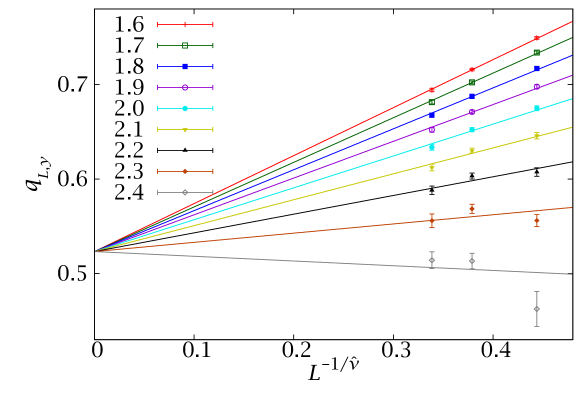
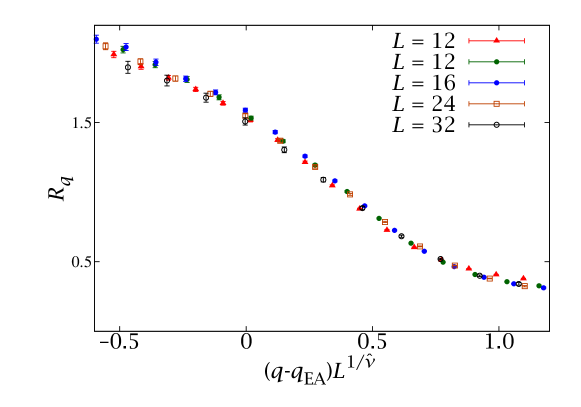
Figure 10.24: Crossing points $q^{(2)}_{L,y}$ computed for pairs of lattices $(L,2L)$ and several values of $y$, against $L^{-1/\hat{\nu}}$. The continuous lines are fits to (10.69) constrained to yield common values of $\hat{\nu}$ and $q_{\text{EA}}$.

Figure 10.25: Scaling plot of the quantity $R_{q}$ of Figure 10.22, using the critical parameters computed in (10.71).

Figure 10.25 shows the result of this fitting procedure. The selection of the number of $y$ is arbitrary: the more $y$ we add, the more degrees of freedom (information) we have, but at the cost of increasing the effects of correlations and endangering the conditioning of the covariance matrix. Fortunately, what seems a delicate choice turns out to be arbitrary, both the fit parameters and their errors being remarkably resilient to changes in the $y_{j}$. For our choice of $y_{j}$ (shown in Figure 10.25), the final results are

$$q_{\text{EA}} =0.52(3), 1/\hat{\nu} =0.39(5),$$ (10.71)

with $\chi^{2}/\text{d.o.f.}=18.9/16$. Notice that our value of $q_{\text{EA}}$ is consistent with the (wide) bounds that we obtained in our preliminary non-equilibrium analysis in Section 10.6.

As pointed out above, the result is very stable to changes in the values of $y$. For instance, removing the $L=8$ data for $y=2.3,2.4$ (the outliers) shifts our final values by one fifth of the error bar. Notice that, from Figure 10.25, $A_{y}^{(2)}$ changes sign at $y\approx 2.35$, so $\theta(q_{\text{EA}})\approx 0.65$. We shall return to this exponent in the next Chapter.

As a test of these critical parameters, we can attempt to produce a scaling plot of the ratio $R_{q}$ that we had plotted in Figure 10.25. This is represented in Figure 10.25, which shows that, indeed, a good collapse is obtained.

Let us finally note that our value of $1/\hat{\nu}=0.39(5)$ is compatible with the best known result for the thermal critical exponent $1/\nu=0.408(25)$ [hasenbusch:08b], so it may be that the two are equal after all. We shall consider other conjectures for $1/\hat{\nu}$ and, in particular, its relation with $\theta(q)$, in Section 11.3.

10.9  The finite-time scaling paradigm

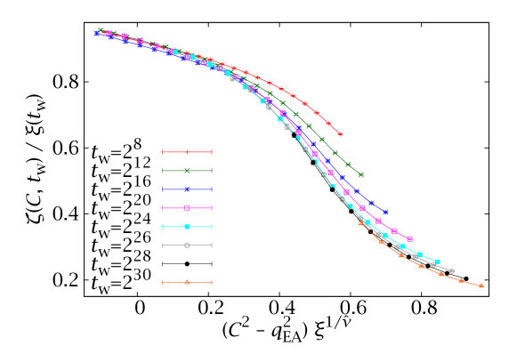
Figure 10.26: Finite-time scaling plot: dimensionless ratio $\zeta(C,t_{\mathrm{w}})/\xi(t_{\mathrm{w}})$ against the scaling variable $(C^{2}-q_{\text{EA}}^{2})\xi(t_{\mathrm{w}})^{1/\hat{\nu}}$.

In the previous section we obtained an important result: the spin-glass order parameter $q_{\text{EA}}$. This had eluded us in our previous non-equilibrium study (Section 10.6) and had also never been done in a controlled way in equilibrium.

We also saw how the critical parameters thus obtained could produce scaling plots of dimensionless observables in equilibrium.

We can now consider a complementary problem. Given the equivalence between $L$ and $\xi(t_{\mathrm{w}})$ through the time-length dictionary, should it not be possible to produce a dynamical scaling plot? The answer turns out to be yes. In Figure 10.26 we have plotted the dimensionless ratio $\zeta(C,t_{\mathrm{w}})/\xi(t_{\mathrm{w}})$ as a function of the scaling variable $(C^{2}-q_{\text{EA}}^{2})\xi(t_{\mathrm{w}})^{1/\hat{\nu}}$. The values of $\hat{\nu}$ and $q_{\text{EA}}$ used were directly those of (10.71). As we can see, we obtain a collapse of the curves for large $t_{\mathrm{w}}$.

Figure 10.26 suggests that the correct manner to treat the statics-dynamics equivalence in a fully quantitative way is to adopt a ‘finite-time scaling’ (FTS) formalism.

The FTS approach provides a natural explanation for the extremely small exponents found in our power-law extrapolation of $C_{\infty}(t)$ (Section 10.6). Indeed, FTS implies that

$$C_{\infty}(t)-q_{\text{EA}}\propto\zeta_{\infty}(t)^{-1/\hat{\nu}},\qquad\zeta_{\infty}(t)=\lim_{t_{\mathrm{w}}\to\infty}\zeta(t,t_{\mathrm{w}}).$$ (10.72)

Finally, we expect

$$\zeta_{\infty}(t)\propto t^{z_{\zeta}},$$ (10.73)

and, in fact, (see Table 10.4) the evidence suggests that $z_{\zeta}$ is equal to the dynamic critical exponent $z$. Therefore, the exponent $B$ of Section 10.6,

$$C_{\infty}(t)=q_{\text{EA}}+At^{-B},$$ (10.47)

is

$$B=\frac{1}{z\hat{\nu}}\approx 0.0325.$$ (10.74)

We have used the value of $z(T=0.7)=12.03(27)$ from Table 10.1. This agrees at least in order of magnitude with the results of Table 10.5 (which is about as much as we could have hoped for, given the problems in estimating $B$ from dynamical data).

We finally note that recent improvements in the experimental measurement of response function with space-time resolution suggest that $\zeta(t,t_{\mathrm{w}})$ may soon be experimentally accessible [oukris:10]. Therefore, our finite-time scaling framework has potential implications for experimental work.

CHAPTER XI   The structure of the $D=3$ spin-glass phase

In this chapter we consider the finer details of the structure of the $D=3$ spin-glass phase. In particular, we try to decide which of the competing theories (RSB, droplet, TNT) offers a best description. To this end, we begin by examining the would-be triviality in the spin and link overlaps which, as we explained in Chapter 9, is the main differentiating characteristic between the three pictures.

This analysis is carried out on the light of our previous results for the statics-dynamics equivalence. In particular, we stress the fact that the theory with most experimental relevance is the effective one at $L\sim 100$, rather than the one that best describes the thermodynamical limit. In this sense, we shall conclude that the RSB framework provides the best picture of the experimental spin glass. Still, this large-$L$ limit is also interesting from a theoretical point of view. Therefore, we also attempt infinite-volume extrapolations, carefully checking for finite-size effects.

We conclude this chapter (and our study of spin glasses) with a detailed analysis of the structure of correlations in the spin-glass phase.

11.1  The spin overlap

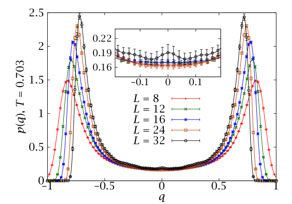
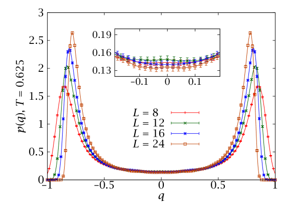
Figure 11.1: Overlap probability density function $p(q)$, Eq. (10.54), at $T=0.625$ and $T=0.703$. Notice that for the central sector of $q\sim 0$ the curves for the different system sizes quickly reach a plateau with $p(q)>0$.

We begin our study by considering the most straightforward observable: the spin overlap $q$. As we explained in Chapter 9, the behaviour of this quantity is one of the clearest markers to distinguish the droplet picture from the RSB one. In particular, droplet predicts a trivial $p(q)$ in the thermodynamical limit (two deltas at $\pm q_{\text{EA}}$), while RSB predicts a non-trivial behaviour (non-zero probability density for all $|q|\leq q_{\text{EA}}$).

We have plotted the $p(q)$ of Eq. (10.54), in Figure 11.1 for $T=0.703$ (the lowest temperature for $L=32$) and for $T=0.625$ (the lowest for $L=24$). The curves are very smooth, thanks to the Gaussian convolution of (10.54). According to the previously mentioned theoretical predictions, one would expect the peaks to get narrower and closer together as $L$ grows. The shift in position is very clear (recall from the previous Chapter that $q_{\text{EA}}$ at $T=0.703$ is $\approx 0.52$) but a more careful analysis is needed to assess the change in width (Section 11.1.2).

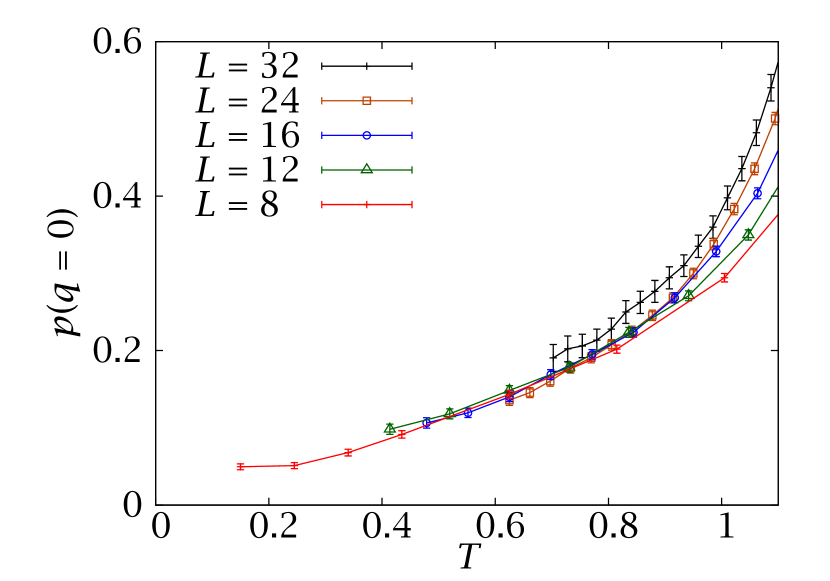
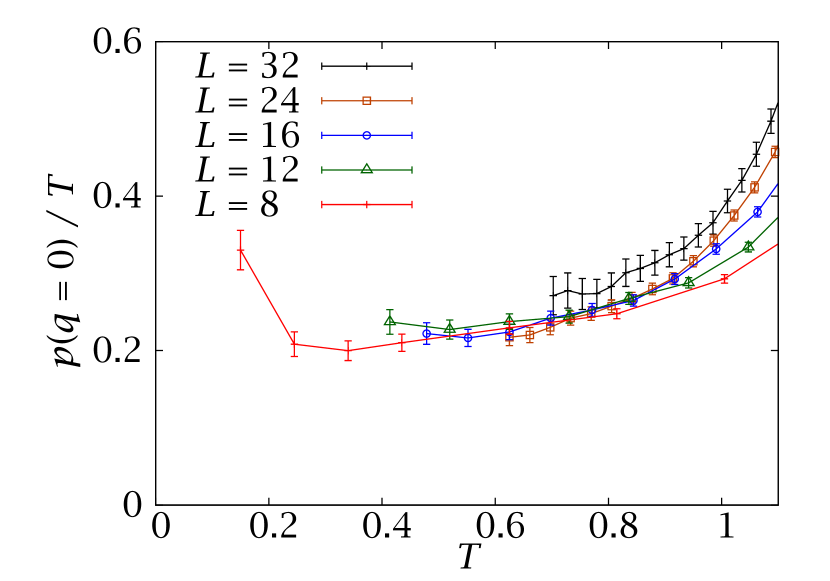
Figure 11.2: Overlap density distribution function at zero overlap as a function of temperature. We observe an enveloping curve with a linear behaviour, as expected in an RSB setting.

In addition, the probability density at $q=0$ shows no evolution, favouring the RSB scenario. In order to see it more clearly we have plotted $p(q=0)$ at $T=0.703$ in Figure 11.2 for all our lattices. We can see a clear non-zero enveloping curve. More precisely, in a mean-field setting one expects this probability density to be linear in $T$ below $T_{\mathrm{c}}$ [mezard:87]. This expectation is checked in the right panel of Figure 11.2. The seemingly out of control value of $p(0)$ at the lowest temperature for $L=8$ is an artifact of the binary nature of the couplings (a finite system always has a finite energy gap). The fact that finite-size effects in $p(0)$ are stronger close to $T=0$ than at finite temperature has been studied in [palassini:01].

From a droplet model point of view, Moore et al. [moore:98] have argued that the apparent lack of a vanishing limit for $p(0)$ in numerical work in the 1990s was an artifact of critical fluctuations. In fact, at $T_{\mathrm{c}}$, $p(0)$ diverges as $L^{\beta/\nu}$ while droplet theory predicts that, for very large lattices, it vanishes with the stiffness exponent $y\approx 0.2$ as $L^{-y}$, for all $T<T_{\mathrm{c}}$. These authors rationalise the numerical findings as a crossover between these two limiting behaviours. However, a numerical study at very low temperatures (so the critical regime is avoided) found for moderate system sizes a non-vanishing $p(0)$ [katzgraber:01]. Furthermore, we shall compute in Section 11.1.2 a characteristic length for finite-size effects in the spin-glass phase, which turns out to be small at $T=0.703$.

In any case, the behaviour at the experimentally relevant scale of $L\sim 100$ seems without a doubt to be non-trivial (there is no room for a change of regime between our simulations and $L\sim 100$).

11.1.1 The Binder cumulant

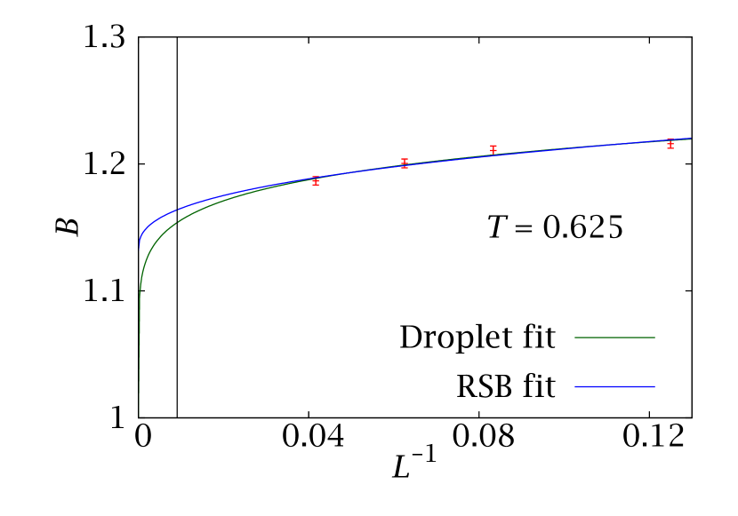
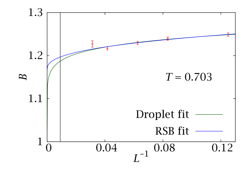
Figure 11.3: Infinite volume extrapolation of the Binder parameter at $T=0.703$ and $T=0.625$ and fits to the behaviour expected in the RSB, Eq. (11.3b), and droplet, Eq. (11.3a), pictures (cf. Table 11.1). For the experimentally relevant scale of $L=110$ (dotted vertical line), both fits are well above the $B=1$ value of a coarsening system.

$T$	Droplet fit				RSB fit
	$\chi^{2}/\mathrm{d.o.f.}$	$a$	$y$		$\chi^{2}/\mathrm{d.o.f.}$	$c$	$d$
0.703	3.78/3	0.312(17)	0.110(17)		3.44/3	1.165(12)[34]	0.186(34)[03]
0.625	2.00/2	0.289(16)	0.134(21)		2.73/2	1.128(11)[33]	0.193(28)[03]

Table 11.1: Scaling of the Binder parameter and fit to the behaviour expected in the droplet, Eq. (11.3a), and RSB pictures, Eq. (11.3b).

We can define the Binder ratio for spin glasses just as we did for the Ising ferromagnet in (5.10)

$$B(T)=\frac{\overline{\braket{q^{4}}}}{\overline{\braket{q^{2}}}^{2}}\,.$$ (11.1)

Notice that we compute these moments from the original $p_{1}(q)$, not from our smoothed version. Above $T_{\mathrm{c}}$ the fluctuations of $q$ are expected to be Gaussian in the large-$L$ limit, hence

$$\lim_{L\to\infty}B(T)=3,\qquad T>T_{\mathrm{c}}.$$ (11.2)

Below $T_{\mathrm{c}}$ the situation of course depends on whether the droplet or the RSB pictures are correct. In the former, $B(T<T_{\mathrm{c}})$ should approach $1$ in the large-$L$ limit (as in a ferromagnet). In the latter, one expects $1<B<3$.

Therefore, we have the following expectations

$$\mathrm{Droplet:}\qquad B(T;L) =1+aL^{-y},$$ (11.3a)

$$\ \ \,\quad\mathrm{RSB:}\qquad B(T;L) =c+dL^{-1/\hat{\nu}}.$$ (11.3b)

The droplet prediction (11.3a) depends on the stiffness exponent $y$, while in the RSB picture the finite-size evolution is controlled by the exponent $1/\hat{\nu}=0.39(5)$, which we computed in the previous Chapter.

We have plotted the Binder ratio for $T=0.703$ and $T=0.625$ in Figure 11.3, along with fits to (11.3). The resulting parameters are gathered in Table 11.1. For the RSB fit we include two error bars: the number enclosed in $(\cdot)$ comes from the statistical error in a fit with fixed $\hat{\nu}$ and the one in $[\cdot]$ is the systematic error due to our uncertainty in $\hat{\nu}$.

As it turns out, both fits have acceptable values of $\chi^{2}/\text{d.o.f.}$. However, the evolution of $B$ with $L$ is very slow, so in order to accommodate the droplet behaviour we have needed a very small exponent $y\approx 0.12$, smaller than the usual droplet prediction of $y\approx 0.2$ [bray:87].

Let us finally note that, again, the extrapolation at $L\sim 100$ is well above one even with the droplet scaling.

11.1.2 The peaks of $p(q)$

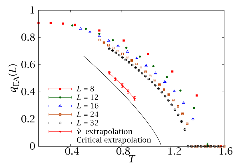
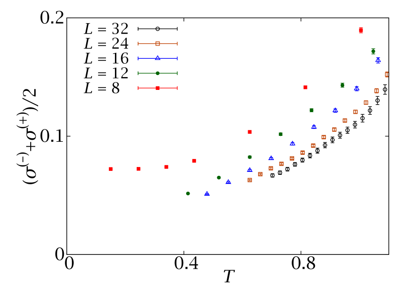
Figure 11.4: Left: $q_{\mathrm{EA}}(L)$ as a function of the temperature. We include two different infinite-volume extrapolations. The first uses the dynamical heterogeneities exponent $1/\hat{\nu}$, cf. (11.5) and (11.3). The second is obtained from finite-size scaling arguments in the critical region, Eqs. (11.10) and (11.13). Right: Width of the peaks of $p(q)$, Eq. (11.4), as a function of $T$ for all our lattice sizes.

$L$	$T=0.703$			$T=0.805$
	$\sigma$	$\sigma p\bigl{(}q_{\mathrm{EA}}(L)\bigr{)}$		$\sigma$	$\sigma p\bigl{(}q_{\mathrm{EA}}(L)\bigr{)}$
8	0.117 7(20)	0.178 4(10)		0.139 1(25)	0.183 3(10)
12	0.096 3(21)	0.174 0(12)		0.116 5(25)	0.180 9(12)
16	0.081 7(16)	0.169 6(11)		0.100 1(22)	0.175 6(11)
24	0.073 5(16)	0.169 0(12)		0.086 0(19)	0.172 8(12)
32	0.066 8(29)	0.163 1(23)		0.079 8(34)	0.166 9(22)
$L_{\mathrm{min}}$	16			16
$\chi^{2}/\mathrm{d.o.f.}$	0.43/1			1.13/1
$B$	$-0.278(28)$			$-0.346(30)$

Table 11.2: Width $\sigma=\bigl{(}\sigma^{(+)}+\sigma^{(-)}\bigr{)}/2$ of the peaks in $p(q)$ and fit to a power law $\sigma(L)=AL^{B}$ in the range $[L_{\mathrm{min}},32]$. We also include the product $\sigma p\bigl{(}q_{\mathrm{EA}}(L)\bigr{)}$.

As we have seen, the droplet and RSB pictures have very different predictions for $p(q)$ as a whole. However, they both agree in that the two symmetric peaks observed at finite $L$ should eventually become two Dirac deltas at $\pm q_{\text{EA}}$, a prediction that we can check.

Let us begin by defining $q_{\text{EA}}(L)$ as the position of the maximum of $p(q;L)$ (in the remainder of this section, we consider all overlaps positive and the pdf symmetrised). Again, our Gaussian smoothing procedure makes this quantity easy to compute (we fit the neighbourhood of the peak to a third-order polynomial, since the peak is very asymmetric).

In order to test that the peak not only tends to $q_{\text{EA}}$, but also gets infinitely narrow, we can employ the half-widths at half height. Defining $q^{(\pm)}$ through $p(q^{(\pm)})=p\bigl{(}q_{\text{EA}}(L)\bigr{)}/2$, we have

$$\sigma^{(\pm)}=\bigl{|}q^{(\pm)}-q_{\text{EA}}(L)\bigr{|}.$$ (11.4)

Notice that, since we are considering the positive peak, $q^{(-)}<q_{\text{EA}}(L)<q^{(+)}$ (that is, $q^{(-)}$ is the inner width and $q^{(+)}$ the outer).

We have plotted $q_{\text{EA}}(L)$ and $\sigma^{(\pm)}$ in the left and right panels of Figure 11.4, respectively. We see that the width of the peaks does decrease slowly with $L$. However, the product $\sigma p\bigl{(}q_{\text{EA}}(L)\bigr{)}$ has a small dependence on $L$ (Table 11.2).

We can now consider the actual value of $q_{\text{EA}}$. Following Section 10.8, we expect

$$q_{\text{EA}}(L,T)=q_{\text{EA}}(T)\left[1+\frac{A(T)}{L^{1/\hat{\nu}}}\right]\,.$$ (11.5)

We cannot perform a three-parameter fit to (11.5), due to the lack of degrees of freedom, but we need to use our previously computed value of $1/\hat{\nu}=0.39(5)$. Similar extrapolations were attempted in [iniguez:96], but with less control on $1/\hat{\nu}$ (and smaller sizes, $L\leq 16$).

We present the values of $q_{\mathrm{EA}}(L)$ and the result of a fit to Eq. (11.5) in Table 11.3. As we can see, the errors due to the uncertainty in the exponent, denoted by $[\,\cdot\,]$, are greater than those caused by the statistical error in the individual points, $(\,\cdot\,)$. In fact, our data admit good fits for a very wide range of values in $1/\hat{\nu}$. For instance, if we try to input the value of the stiffness exponent obtained in the droplet-like extrapolation of the Binder parameter, $y\sim 0.12$ (see Eq. (11.3a) and Table 11.1), we still obtain a good fit, even though the extrapolated value for $q_{\mathrm{EA}}$ is almost zero at $T=0.703$ and negative at $T=0.805$. Therefore, using the droplet exponent $y$ the spin-glass phase would be non-existent.

$L$	$T=0.703$	$T=0.805$
8	0.824 61(83)	0.781 8(11)
12	0.793 33(85)	0.741 2(11)
16	0.773 00(75)	0.716 81(95)
24	0.740 27(71)	0.679 05(83)
32	0.717 4(14)	0.65 35(16)
$L_{\mathrm{min}}$	16	16
$\chi^{2}/\mathrm{d.o.f.}$	1.83/1	0.98/1
$q_{\mathrm{EA}}$	0.538[22](6)	0.447[24](6)
Section 10.6	$0.474\leq q_{\mathrm{EA}}\leq 0.637$	$0.368\leq q_{\mathrm{EA}}\leq 0.556$

Table 11.3: Extrapolation to infinite volume of $q_{\mathrm{EA}}(L,T)$ using the replicon exponent, Eq. (11.5). We also include the confidence interval previously obtained in the non-equilibrium study of Section 10.6. The resulting estimate for $T=0.703$ is compatible with our previous determination from the phase transition in the dynamical heterogeneities in Section 10.8.

Also included in Table 11.3 is the confidence interval for this observable computed from non-equilibrium considerations in Section 10.6. Notice that the equilibrium values are much more precise, but consistent. The extrapolations included in this table (and analogous ones for other values of $T$) are plotted in Figure 11.4. Finally, notice that the estimate of $q_{\text{EA}}(T=0.703)$ in Table 11.3 is compatible with our value of $q_{\text{EA}}(T=0.703)=0.52(3)$, obtained in Section 10.8 with a completely different method.

11.1.3 Critical and finite-size effects

In order for our extrapolations to the thermodynamical limit to be meaningful, we have to check that we are not in a preasymptotic regime dominated by critical fluctuations. This is best done through a finite-size scaling analysis of the $p(q)$.

$T$	$L_{\mathrm{c}}^{1/\hat{\nu}}$	$L_{\mathrm{c}}$	$L_{\mathrm{c}}(T_{\mathrm{c}}-T)^{\nu}$
0.703	1.253[20](32)	1.78[8](11)	0.197[8](13)
0.75	1.448[24](34)	2.58[12](16)	0.210[8](13)
0.805	1.731[28](44)	4.08[18](27)	0.221[10](15)
0.85	2.023[32](54)	6.09[26](42)	0.222[10](15)
0.90	2.514[41](66)	10.63[44](71)	0.230[10](15)

Table 11.4: Determination of $L_{\mathrm{c}}$ from the fits to Eq. (11.5), using (11.8), for several temperatures below $T_{\mathrm{c}}$. Errors are given as in Table 11.3. The characteristic length $L_{\mathrm{c}}(T)$ scales as a correlation length when $T$ approaches $T_{\mathrm{c}}$ ($\nu\approx 2.45$ from [hasenbusch:08b]). We warn the reader that the $\chi^{2}/\mathrm{d.o.f.}$ for the fits at $T=0.85$ and $0.90$ are, respectively, $2.6/1$ and $2.7/1$.

Let us first show that our estimate of $q_{\text{EA}}$ provides a determination of the correlation length in the spin-glass phase. Notice that we are in a situation were the correlations decay algebraically, so the concept of correlation length is delicate [josephson:66]. In particular, finite-size effects are ruled by a crossover length $L_{\text{c}}(T)$, scaling as a correlation length: $L_{\text{c}}\propto(T_{\text{c}}-T)^{-\nu}$. In fact, one would expect

$$\frac{q_{\text{EA}}(T,L)}{q_{\text{EA}}(T)}=1+h[L/L_{\text{c}}(T)].$$ (11.6)

We do not know the complete crossover function $h$, but we do know that for large $x$ it should behave as $h(x)\sim x^{-1/\hat{\nu}}$, so we make the simplest ansatz,

$$h(x)=x^{-1/\hat{\nu}}.$$ (11.7)

Then, if we compare (11.6) with (11.5), we see that the amplitude of the finite-size corrections in the latter can be written as

$$A(T)=[L_{\text{c}}(T)]^{1/\hat{\nu}}.$$ (11.8)

The resulting values of $L_{\text{c}}$ can be seen in Table 11.4. Notice that this crossover length does scale with temperature as expected for the bulk behaviour, which constitutes a weighty argument for the asymptotic nature of our results.

In order for our previous extrapolations for $q_{\text{EA}}$ to be valid, we need to stay in a temperature regime where $L\gg L_{\text{c}}(T)$, a condition that is amply satisfied for our working temperatures of $T=0.703$ and $T=0.805$.

In the region close to $T_{\text{c}}$, where $L$ becomes smaller than $L_{\text{c}}(T)$, we can use finite-size scaling to extrapolate $q_{\text{EA}}(T)$. This somewhat unconventional use of finite-size scaling was started in [luescher:91, kim:93, caracciolo:95, caracciolo:95b] and has also been used in the spin-glass context [palassini:99, jorg:06]. Most of the times, these ideas are used in the paramagnetic phase, but we show below how to implement them in the low-temperature phase.

Close to $T_{\mathrm{c}}$, we know that

$$q_{\mathrm{EA}}^{\infty}(T)=\lambda(T_{\mathrm{c}}-T)^{\beta}[1+\mu(T_{\mathrm{c}}-T)^{\omega\nu}+\ldots]\,.$$ (11.9)

We have excellent determinations of $T_{\mathrm{c}}$ and $\beta$ from the work in [hasenbusch:08b], so we need only estimate the amplitude $\lambda$. In fact, Wegner’s confluent corrections $(T_{\mathrm{c}}-T)^{\omega\nu}$ are small close to $T_{\mathrm{c}}$. To proceed, we note that finite-size scaling tells us that

$$q_{\mathrm{EA}}(L,T)=L^{-\beta/\nu}F(x)[1+L^{-\omega}G(x)+\ldots],\qquad x=L^{1/\nu}(T_{\mathrm{c}}-T),$$ (11.10)

where the critical exponents are (from [hasenbusch:08b]),

$$\nu=2.45(15),\qquad\beta=0.77(5),\qquad\omega=1.0(1).$$ (11.11)

In order to connect Eq. (11.10) with the infinite-volume limit in Eq. (11.9) the asymptotic behaviour of the scaling functions $F(x)$ and $G(x)$ must be for large $x$

$$F(x)\sim x^{\beta},\qquad G(x)\sim x^{\omega\nu}.$$ (11.12)

The resulting scaling plot is represented in Figure 11.5. Varying the values of $T_{\mathrm{c}}$ and the critical exponents inside their error margins does not make significant changes in the plot. Notice how the curves collapse for small values of the scaling variable $x$ and large $L$, but how for our lowest temperatures scaling corrections become important. In fact, Eq. (11.10) implies that when the temperature is lowered away from $T_{\mathrm{c}}$ the amplitude for scaling corrections grows as $x^{\omega\nu}\approx x^{2.45}$.

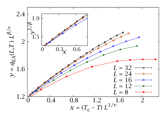
Figure 11.5: Scaling plot of $y=q_{\mathrm{EA}}(L,T)L^{\beta/\nu}$ in the critical region below $T_{\mathrm{c}}$, following Eq. (11.10) and using the values given in [hasenbusch:08b] for the critical exponents and $T_{\mathrm{c}}$. Inset: Close-up of the region near $T_{\mathrm{c}}$ in the representation of Eq. (11.13), showing a linear behaviour for large $L$.

In order to estimate the amplitude $\lambda$ we shall concentrate on the small-$x$ region where finite-size scaling corrections are smallest. Disregarding scaling corrections in (11.10),

$$\bigl{(}q_{\mathrm{EA}}(L,T)L^{\beta/\nu}\bigr{)}^{1/\beta}=F(x)^{1/\beta}\ \underset{x\to\infty}{\longrightarrow}\ x.$$ (11.13)

The inset of Figure 11.5 shows that we reach this asymptotic behaviour for $L\geq 24$. Then, using the simplest parameterisation, $F(x)=(\lambda^{1/\beta}x+B)^{\beta}$,

$$q_{\mathrm{EA}}(L,T)=\lambda(T_{\mathrm{c}}-T)^{\beta}\left[1+\frac{\beta B}{\lambda^{1/\beta}(T_{\mathrm{c}}-T)L^{1/\nu}}+\ldots\right]\ .$$ (11.14)

We can fit our $L=32$ data for $x<0.4$ (where the curves for $L=24$ and $L=32$ are compatible) and use the resulting value of $\lambda$ to extrapolate in Eq. (11.14) to infinite volume. This extrapolation is represented as a function of $T$ in Figure 11.4. It is clear that this critical extrapolation differs with the extrapolation from (11.5) at most by two standard deviations. The difference, if any, could be explained as Wegner’s confluent corrections. However, to make any strong claim on confluent corrections, one would need to estimate the error in the critical extrapolation. Unfortunately, we have found that this error estimate is quite sensitive to the statistical correlation between $T_{\mathrm{c}}$, $\nu$, and $\beta$ (as far as we know, the corresponding covariance matrix has not been published).

One could be tempted to compare Eq. (11.14) with Eq. (11.5) and conclude $\hat{\nu}=\nu$. In the previous Chapter we observed that, at the numerical level, $\nu=2.45(15)$ [hasenbusch:08b] and $\hat{\nu}=2.6(3)$. However, we do not regard this as fireproof. Indeed, it is a consequence of our somewhat arbitrary parameterisation $F(x)=(\lambda^{1/\beta}x+B)^{\beta}$. To investigate this issue further, the small-$x$ region is not enough. One is interested in the asymptotic behaviour of $F(x)$ for large $x$ where unfortunately corrections to scaling are crucial. A careful study of the crossover region can be done only by considering corrections to scaling both at the critical temperature (at $q=0$) and below the critical temperature (at $q=q_{\mathrm{EA}}$).

Finally, the reader could worry about the applicability of (11.9) well below $T_{\mathrm{c}}$. The issue has been considered recently within the framework of droplet theory [moore:10]. It was found that (11.9) is adequate for all $T<T_{\mathrm{c}}$ (actually, no Wegner’s scaling corrections were discussed in [moore:10]). Thus, the fact that our data are describable as scaling behaviour with leading Wegner’s correction does not imply that they are not representative of the low-temperature phase.

11.2  The link overlap and overlap equivalence

In the previous section we showed that our numerical simulations favour a non-trivial scenario for the spin overlap, at least for experimentally relevant scales. This is strong evidence against the droplet picture of the spin-glass phase, but still leaves undecided the issue of TNT vs. RSB.

The difference between these two theoretical descriptions is best examined through the link overlap, introduced in Section 9.2.3. In the notation of real replicas $\{s_{\boldsymbol{x}}^{(1)}\}$ and $\{s_{\boldsymbol{x}}^{(2)}\}$, this is

$$Q_{\text{link}}=\frac{1}{N_{\text{l}}}\sum_{\braket{{\boldsymbol{x}},{\boldsymbol{y}}}}s_{\boldsymbol{x}}^{(1)}s_{\boldsymbol{y}}^{(1)}s_{\boldsymbol{x}}^{(2)}s_{\boldsymbol{y}}^{(2)}.$$ (11.15)

Notice that in a system of $D$ spatial dimensions, the number of links is $N_{\text{l}}=ND$. Also,

$$C_{4}(r\!=\!1)=\overline{\braket{Q_{\text{link}}}}.$$ (11.16)

The link overlap is arguably a better fundamental quantity to describe the spin-glass phase in $D=3$ than $q$ [marinari:99, contucci:05b, contucci:06]. First, as was explained in Section 9.2.3, it is more sensitive than $q$ to the differences between RSB and the other theoretical scenarios for the spin-glass phase (RSB expects a non-trivial behaviour for $Q_{\text{link}}$, which is trivial in both the droplet and TNT pictures). Second, while $Q_{\text{link}}$ is just $q^{2}$ in the mean-field model, the link overlap is actually more amenable than $q$ to an analytical treatment in $D=3$ (within the RSB framework) [contucci:03, contucci:05, contucci:07]. In particular, $Q_{\text{link}}$ is a more convenient quantity to study some properties of the spin-glass phase such as replica equivalence [parisi:98, parisi:00] or ultrametricity [contucci:07b].

In short, for RSB system we expect to have overlap equivalence: fixing $q^{2}$ should also fix $Q_{\text{link}}$, even if the relation between these two observables in $D=3$ is something other than an identity.

In this section we shall study the issue of overlap equivalence using both a non-equilibrium and an equilibrium approach.

11.2.1 Non-equilibrium study

From a non-equilibrium point of view, we can consider the two-time link overlap

$$C_{\text{link}}(t,t_{\mathrm{w}})=\frac{1}{DN}\overline{\sum_{\braket{{\boldsymbol{x}},{\boldsymbol{y}}}}c_{\boldsymbol{x}}(t,t_{\mathrm{w}})c_{\boldsymbol{y}}(t,t_{\mathrm{w}})},$$ (11.17)

where $c_{\boldsymbol{x}}(t,t_{\mathrm{w}})$ was defined in (10.7). Using the usual substitution of $C^{2}$ for $t$ as independent variable, we can explore the would-be differences in the aging of the spin and link overlap with this equations and, hence, distinguish between the coarsening dynamics of droplet and TNT and the non-coarsening evolution of RSB. The analogue to Eq. (10.10) is now

$$\overline{\braket{Q_{\text{link}}}}=\lim_{t\to\infty}\lim_{t_{\mathrm{w}}\to\infty}C_{\text{link}}(t,t_{\mathrm{w}})=\lim_{C^{2}\to 0}\lim_{t_{\mathrm{w}}\to\infty}C_{\text{link}}\bigl{(}t(C^{2},t_{\mathrm{w}}),t_{\mathrm{w}}\bigr{)}.$$ (11.18)

In particular, for a coarsening system, $C_{\text{link}}(C^{2},t_{\mathrm{w}})$ should be independent of $C^{2}$ for $C^{2}<q_{\text{EA}}^{2}$ and large $t_{\mathrm{w}}$. Indeed, in this regime, the relevant system excitations are the reversal of coherent domains where the overlap is already $q_{\text{EA}}$ (as low as it can get, since there are no states for smaller $|q|$). Since these domains have a vanishing surface-to-volume ratio (cf. Section 9.2.3), these excitations do not induce a finite change in $C_{\text{link}}$, even if they do modify $C^{2}$. Therefore, in the large-$t_{\mathrm{w}}$ limit, $C_{\text{link}}$ should reach its equilibrium value $\overline{\braket{Q_{\text{link}}}}$ at $C^{2}=q_{\text{EA}}^{2}$ and not decrease any further. This behaviour is illustrated in Figure 11.6, showing the $C_{\text{link}}(C^{2},t_{\mathrm{w}})$ of the $D=2$ Ising model (the most straightforward coarsening system).

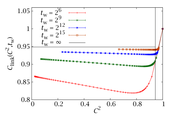
Figure 11.6: Plot of $C_{\text{link}}(C^{2},t_{\mathrm{w}})$ for the $D=2$ Ising model at $T=0.66T_{\text{c}}$ (results from simulations of an $L=4096$ system, averaged over $20$ thermal histories). Below $C^{2}=q_{\text{EA}}^{2}$ the function approaches a $C$-independent value for long times —here $q_{\text{EA}}=m_{\text{Y}}^{2}$, where $m_{\text{Y}}$ is Yang’s magnetisation (5.13).

On the other hand, the overlap equivalence property of the RSB picture translates into an equal aging for $C$ and $C_{\text{link}}$. Here, when $C^{2}$ decreases below $q_{\text{EA}}^{2}$ it is because new states are constantly being found, involving a change of a domain with a volume-filling surface and, hence, changing $C_{\text{link}}$. Therefore, $C_{\text{link}}$ is a non-constant function of $C^{2}$ for the whole range (again, for the Sherrington-Kirkpatrick model, $C_{\text{link}}=C^{2}$).

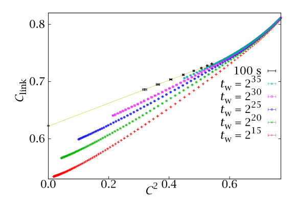
Figure 11.7: Plot of $C_{\text{link}}(C^{2},t_{\mathrm{w}})$ for our spin-glass simulations at $T=0.6$. The behaviour for our simulated times reproduces a non-coarsening behaviour, even if the slope decreases with increasing $t_{\mathrm{w}}$. We also show an extrapolation for a typical experimental time of $100$ s, which is still far from the coarsening behaviour of Figure 11.6.

Let us see where our simulations stand. We have plotted the $C_{\text{link}}(C^{2},t_{\mathrm{w}})$ of the Edwards-Anderson spin glass at $T=0.6$ in Figure 11.7. The behaviour at our finite times seems to reproduce the RSB prediction. Still, the slope of the curve decreases (slowly) when $t_{\mathrm{w}}$ increases.

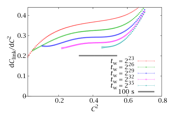
Figure 11.8: Derivative of the link correlation function, regarded as a function of $C^{2}$, for our spin-glass simulations at $T=0.6$. For fixed $C^{2}$, the derivative decreases with time but an extrapolation to an experimental scale of $100$ s is well above zero (grey line, the width represents our error bars).

In order to analyse this behaviour more quantitatively, we have interpolated the link correlation function at fixed $t_{\mathrm{w}}$ with the lowest-order polynomial that allowed a fair fit (seventh order for $t_{\mathrm{w}}\lesssim 2^{35}$, sixth for longer times, where we cover a smaller $C^{2}$ range). We then computed $\mathrm{d}C_{\text{link}}/\mathrm{d}(C^{2})$ by differentiating the interpolating polynomial (Figure 11.8).

Notice that for small $C^{2}$ the derivative seems to reach a plateau for a widening $C^{2}$ range (suggesting that the relation between $C_{\text{link}}$ and $C^{2}$ becomes linear, as in the mean-field model).

Now, we would like to extrapolate these correlation functions and their derivatives to an experimentally relevant time scale, to see whether or not they reach the coarsening behaviour. In order to do this, we consider $C(rt_{\mathrm{w}},t_{\mathrm{w}})$ and $C_{\text{link}}(rt_{\mathrm{w}},t_{\mathrm{w}})$ for $r=8,4,\ldots,\frac{1}{16}$ and fit each of these functions to $a_{r}+b_{r}t_{\mathrm{w}}^{-c_{r}}$. The parameters are stable to variations in the fitting range, as long as $t_{\mathrm{w}}>10^{5}$ and $c_{r}\approx 0.5$. We then use the fits to extrapolate both the link and spin correlation functions to $t_{\mathrm{w}}=10^{14}\sim 100$ s. Additionally, recalling (11.18), the limiting behaviour for $C^{2}=0$ is estimated by extrapolating $\overline{Q_{\text{link}}}(t_{\mathrm{w}})$ to the same experimental time. The resulting $C_{\text{link}}(C^{2},t_{\mathrm{w}}=10^{14})$ is plotted with black crosses in Figure 11.7. The computed points fall on a straight line, whose slope we can use to estimate the derivative $\mathrm{d}C_{\text{link}}/\mathrm{d}(C^{2})|_{t_{\mathrm{w}}=10^{14}}$. This is plotted in Figure 11.8 with a thick grey line (the width of the line represents our error interval).

In short, the behaviour at a typical experimental time is still far from that of a coarsening system. One could be tempted to use the same procedure to extrapolate to $t_{\mathrm{w}}\to\infty$, but the resulting errors are so large as to permit any kind of behaviour.

We need some more theoretical input on the scaling of $C_{\text{link}}$ in the coarsening scenario in order to consider the infinite-time extrapolation.

We consider a large droplet of size $\xi(t+t_{\mathrm{w}})$ at time $t+t_{\mathrm{w}}$ that, at time $t_{\mathrm{w}}$, was made of ${\mathcal{N}}_{\text{C}}$ smaller droplets of size $\xi(t_{\mathrm{w}})$. The number of spins in the droplet’s boundary scales as $\xi(t_{\mathrm{w}})^{D_{\text{s}}}$. In a simple coarsening system (such as a ferromagnet), $D_{\text{s}}=D-1$, but we can actually have $D-1\leq D_{\text{s}}<D$ [fisher:88, mcmillan:84, bray:87, fisher:86, fisher:88b]. In fact, the numerical simulations carried out in the TNT framework expect $D-D_{\text{s}}\approx 0.44$ [palassini:00, palassini:03] in $D=3$.

The scaling of ${\mathcal{N}}_{\text{C}}$ is straightforward: ${\mathcal{N}}_{\text{C}}\sim[\xi(t+t_{\mathrm{w}})/\xi(t_{\mathrm{w}})]^{D}$. The overlap of each of the droplets at time $t_{\mathrm{w}}$ with the combined droplet at $t+t_{\mathrm{w}}$ is randomly $\pm q_{\text{EA}}$. Therefore, one expects

$$C(t,t_{\mathrm{w}})\sim\sqrt{{\mathcal{N}}_{\text{C}}}\left(\frac{\xi(t_{\mathrm{w}})}{\xi(t+t_{\mathrm{w}})}\right)^{D}\sim\left(\frac{\xi(t_{\mathrm{w}})}{\xi(t+t_{\mathrm{w}})}\right)^{D/2}\,.$$ (11.19)

This equation is intuitively evident, but we note that for an Ising ferromagnet (the paragon of coarsening models) it can be actually obtained with an explicit computation. Indeed, for an Ising model, it is shown in [cugliandolo:94] can be written as a series in a parameter $y$, where

$$y=\frac{\xi(t+t_{\mathrm{w}})^{D/2}\xi(t_{\mathrm{w}})^{D/2}}{\bigl{[}\xi(t+t_{\mathrm{w}})^{2}+\xi(t_{\mathrm{w}})\bigr{]}^{D/2}}\,.$$ (11.20)

Equation (11.19) then follows in the $\xi(t+t_{\mathrm{w}})\gg\xi(t_{\mathrm{w}})$ limit.

As to the link overlap, we expect

$$C_{\text{link}}(t,t_{\mathrm{w}})=C_{\text{link}}^{0}+{\mathcal{N}}_{\text{C}}\frac{\xi(t_{\mathrm{w}})^{D_{\text{s}}}}{\xi(t+t_{\mathrm{w}})^{D}}\,.$$ (11.21)

That is, $C_{\text{link}}$ cannot decrease below some finite value $C_{\text{link}}^{0}$, which is nothing but the equilibrium value $\overline{\braket{Q_{\text{link}}}}$. The excess over this value at finite $t$ comes from the probability that a link belong to the surface of a droplet at time $t_{\mathrm{w}}$.

We can now rewrite (11.19) in the form

$${\mathcal{N}}_{\text{C}}\sim\frac{g(C)}{C^{2}}\,,$$ (11.22)

where $g(x)$ is some continuous positive function, not necessarily differentiable at $x=0$. Combining the previous expressions we can rewrite (11.21) as

$$C_{\text{link}}(t,t_{\mathrm{w}})=C_{\text{link}}^{0}+C^{1}_{\text{link}}g(C)\xi(t_{\mathrm{w}})^{D_{\text{s}}-D}.$$ (11.23)

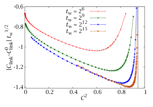
Figure 11.9: Check of (11.23) for the Ising model (the vertical line is $C=q_{\text{EA}}$).

This equation explains the behaviour observed in Figure 11.6 for the Ising ferromagnet. For this system, the $D-D_{\text{s}}=1$, so we would expect $C_{\text{link}}(C^{2},t_{\mathrm{w}})-C_{\text{link}}^{0}$ to scale with $\xi^{-1}$. In Figure 11.9 we can see that this is indeed the case —notice that for the Ising model the coherence length scales as $t_{\mathrm{w}}^{1/2}$ see, e.g., [bray:94].

Equation (11.23) suggests plotting $\mathrm{d}C_{\text{link}}/\mathrm{d}(C^{2})|_{C=C_{*}}$ against $\xi^{-1}(t_{\mathrm{w}})$ and against $\xi^{-0.44}(t_{\mathrm{w}})$ (see Figure 11.10). It is important to choose a value $C_{*}^{2}$ below $q_{\text{EA}}$ but not too small, because otherwise the numerical derivative would be unreliable for lack of data. Therefore, we have chosen values smaller than, but close to, our lower bound for $q_{\text{EA}}$ in Section 10.6. The two representations are linear within our errors. However, while a $\xi^{-1}(t_{\mathrm{w}})$ scaling compatible with standard coarsening seems falsified (i.e., its extrapolation is well above zero), the TNT scaling of $\xi^{-0.44}(t_{\mathrm{w}})$ does extrapolate close to zero with our data.

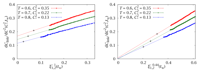
Figure 11.10: Plot of $\mathrm{d}C_{\text{link}}/\mathrm{d}(C^{2})$ against $\xi^{D-D_{\text{s}}}$ for $D_{\text{s}}=2$ (standard coarsening, left) and $D_{\text{s}}=2.55$ (TNT scaling, right). We compute the derivatives at a value of $C_{*}$ below our lowest estimate for $q_{\text{EA}}$ at each temperature. We also mark by crosses our extrapolations to an experimental scale of $100$ s.

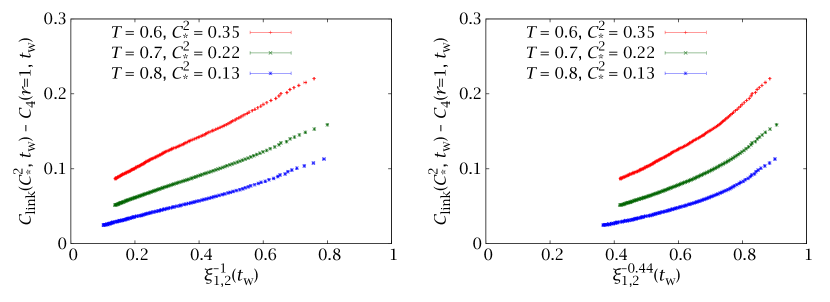
Figure 11.11: Difference $C_{\text{link}}(C^{2}_{*},t_{\mathrm{w}})-C_{4}(r\!=\!1,t_{\mathrm{w}})$ against $\xi^{D_{\text{s}}-D}$ using the same values for $C_{*}$ and $D_{\text{s}}$ as in Figure 11.10. An extrapolation to zero seems unlikely even in the $\xi^{-0.44}$ case.

It is also interesting to attempt a similar representation to Figure 11.9 for the Edwards-Anderson model. Unlike the Ising case, now we do not know the exact value of $C_{\text{link}}^{0}$. However, by definition,

$$\lim_{t_{\mathrm{w}}\to\infty}\overline{Q_{\text{link}}}(t_{\mathrm{w}})=\overline{\braket{Q_{\text{link}}}}=C_{\text{link}}^{0}.$$ (11.24)

Of course, $\overline{Q_{\text{link}}}(t_{\mathrm{w}})=C_{4}(r\!=\!1,t_{\mathrm{w}})$. Then, following (11.23), in a coarsening system

$$C_{\text{link}}(C^{2}_{*},t_{\mathrm{w}})-C_{4}(r\!=\!1,t_{\mathrm{w}})\sim\xi(t_{\mathrm{w}})^{D_{\text{s}}-D},\qquad C_{*}^{2}<q_{\text{EA}}^{2}.$$ (11.25)

We have plotted this difference in Figure 11.11 for a value of $C_{*}$ below our lower bound for $q_{\text{EA}}$ in Section 10.6. Again, we represent both the standard $\xi^{-1}$ scaling and the TNT scaling of $\xi^{-0.44}$. From the first one, it is easy to find a smooth extrapolation to a positive difference. However, now the data are more precise than in Figure 11.10 and the TNT scaling of $\xi^{-0.44}$ does not fit our data and would only be possible if the whole of our simulation were in a preasymptotic regime.

There is another problem with the TNT scaling and it is that (11.23) relies on (11.19), an equation that is disproved by our computation of exponent $d$ in Section 10.4 —we obtained $d\approx 2$, rather the $d=3/2$ compatible with (11.19).

In short, the infinite-time extrapolations remain inconclusive, leaving room for a TNT-like coarsening behaviour. However, in all cases the extrapolations to the experimentally relevant time scale, much safer, show that the dynamics is certainly non-coarsening there (thick line in Figure 11.8 and crosses in Figure 11.10).

11.2.2 Equilibrium study

We can attempt an analogous study with our equilibrium simulations. The role of $C_{\text{link}}(C^{2},t_{\mathrm{w}})$ is now played by $\mathrm{E}(Q_{\text{link}}|q)$, where the conditional expectation value was defined in (10.56).

Just as in the non-equilibrium case, we expect $Q_{\text{link}}$ to be a strictly increasing function of $q^{2}$ below $q_{\text{EA}}^{2}$ for an RSB system, and to be constant for a TNT system. Now the large-$t_{\mathrm{w}}$ limit is of course replaced by a large-$L$ limit and the experimental scale is, as always, $L\sim 100$.

In Table 11.5 we give $C_{4}(r\!=\!1|q\!=\!0)$ and $C_{4}(r\!=\!1|q\!=\!0.523)$ for our simulations at $T=0.7$ (where $q_{\text{EA}}=0.523(32)$, from Section 10.8). According to the TNT picture, these two quantities should scale as $L^{-0.44}$ and have the same extrapolation to infinite $L$. As the reader can check, however, the data do not fit the $L^{-0.44}$ behaviour, let alone extrapolate to the same large-$L$ limit. The same conclusion holds if we replace $L$ by

$$\ell=\uppi/\sin(\uppi/L),$$ (11.26)

more natural for lattice systems. Yet, it could be argued that our data are preasymptotic, so we may try a TNT extrapolation with corrections to scaling

$$C_{4}(r\!=\!1|q)=C_{\infty}+A_{q}L^{-0.44}(1+B_{q}L^{-x}).$$ (11.27)

We have performed a joint fit of the data from Table 11.5 to this equation, using a chi-square estimator analogous to that of (10.70). The fit parameters are the four amplitudes $A_{0},B_{0},A_{0.523},B_{0.523}$, the common scaling corrections exponent $x$ and the common extrapolation $C_{\infty}$. In this case the correlation of the data for $q=0$ and $q=0.523$ at the same $L$ is very small —see Table 11.5— and, of course, there is no correlation between data at different $L$. The result is

$$C_{\infty} =0.677_{-0.005}^{+0.012}, x =0.57^{+0.26}_{-0.08}, \chi^{2}/\text{d.o.f.} =9.1/4.$$ (11.28)

Notice the highly asymmetric errors. The fit is not a very good one, its $\mathcal{P}$-value (cf. Appendix B) is of only $6~{}\%$.

$L$	$C(1|0)$	$C(1|q_{\mathrm{EA}})$	$\mathcal{R}$
8	0.46138(82)	0.57253(33)	0.134
12	0.51649(71)	0.60390(28)	0.051
16	0.54552(60)	0.62089(22)	0.060
24	0.57573(77)	0.63742(17)	$-0.119$
32	0.59131(94)	0.64579(24)	0.063

Table 11.5: $C(r=1|q)$ for $q=0$ and $q=q_{\mathrm{EA}}$ for all our system sizes at $T=0.703$. For each $L$, we include the correlation coefficient between both values of $q$.

Therefore, the TNT behaviour is seen to be, at best, very forced with our numerical data. In the RSB setting, however, we expect $C_{4}(r\!=\!1|q)$ to scale as $\sim L^{-1}$, with a $q$-dependent infinite volume value $C_{\infty}(q)$. Indeed, if we fit the data in Table 11.5 to $C(1|q)=C_{\infty}(q)+A/\ell$ we obtain

$$C_{\infty}(0) =0.634\,9(8), \chi^{2}/\text{d.o.f.} =3.63/3,$$ (11.29)

$$C_{\infty}(q_{\text{EA}}) =0.671\,1(2), \chi^{2}/\text{d.o.f.} =2.86/3.$$ (11.30)

Using $L$ instead of $\ell$, we would have had to restrict the fit to the largest lattices, but the results would be similar (if with larger errors), as the reader can easily check.

11.2.2.1 The variance of the link overlap

We have seen that $Q_{\text{link}}$ is a strictly increasing function of $q^{2}$. However, in order for these two variables to be interchangeable, we need a second condition. That is, the conditional variance of $Q_{\text{link}}$ at fixed $q$ must vanish in the large-$L$ limit. In this way, fixing $q$ would unambiguously fix $Q_{\text{link}}$ also.

In general, we define the conditional variance of $O$ at fixed $q=c$ as

$$\mathrm{Var}(O|q=c)=\mathrm{E}(O^{2}|c)-\mathrm{E}(O|c)^{2}.$$ (11.31)

Notice that

$$\overline{\braket{O^{2}}}-\overline{\braket{O}}^{2}=\int_{-\infty}^{\infty}\mathrm{d}q\ p(q)\bigl{[}\mathrm{Var}(O|q)+\bigl{(}\mathrm{E}(O|q)-\overline{\braket{O}}\bigr{)}^{2}\bigr{]}.$$ (11.32)

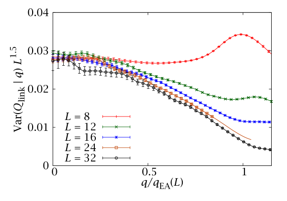
Figure 11.12: Conditional variance $\mathrm{Var}(Q_{\text{link}}|q)$ for all our lattice sizes at $T=0.703$. We rescale the horizontal axis by the $q_{\text{EA}}(L)$, in order to see a better collapse.

In Figure 11.12 we plot $\mathrm{Var}(Q_{\text{link}}|q)$ for all our lattice sizes at $T=0.703$. We find a very clear decay of the variance. The decay exponent $\mathrm{Var}(Q_{\text{link}}|q)\sim L^{-c}$ is compatible with $c=D/2$, although we lack a theoretical argument for this particular value.

11.3  The structure of correlations in the spin-glass phase

In the previous sections we examined two of the most straightforward characteristics of the spin-glass phase: the question of (non)-triviality in the spin and link overlaps. We interpreted our study as a way of distinguishing between the three competing pictures of the spin-glass phase: droplet, TNT and RSB.

Of the three, RSB fit our finite-size data better and also produced more consistent extrapolations to the thermodynamical limit (assuming our data are representative of the asymptotic behaviour, a possibility supported by Section 10.3.2). In any case, even accepting the possibility of a crossover at very large sizes that would completely change the behaviour in the thermodynamical limit, the conclusion that the RSB picture describes the spin-glass phase at the experimentally relevant scale of $L\sim 100$ seems safe.

Still, stating that the RSB framework seems more faithful to the physics of the Edwards-Anderson model would not end the discussion. Recall that this theory was introduced as the solution of the mean-field version of the Edwards-Anderson model. In $D=3$ its more general points (such as the non-triviality of the spin and link overlaps studied thus far) are expected to remain valid, but many fine details are certain to change.

Among these we have the issue of the structure of the correlations in the spin-glass phase. In Section 10.8 we said that the connected correlation function of an RSB system was expected to decay as $C_{4}(\boldsymbol{r}|q^{2}\leq q_{\text{EA}}^{2})-q^{2}\sim r^{-\theta(q)}$, where the structure exponent $\theta(q)$ is positive for $0\leq|q|\leq q_{\text{EA}}$. This clustering property is a consequence of the existence of the replicon, a critical Goldstone mode. In particular, the RSB result above the upper critical dimension $(D>6)$ is [dedominicis:98, dedominicis:99]

$$\theta(q=0) =D-4,$$ (11.33a)

$$\theta(0<|q|<q_{\text{EA}}) =D-3.$$ (11.33b)

$$\theta(|q|=q_{\text{EA}}) =D-2.$$ (11.33c)

These results are expected to renormalise in lower dimensions [dedominicis:06]. In particular, if we want the spin-glass phase to have the clustering property, these values are inconsistent in $D<4$ (because then the correlation function would grow with distance). On the other hand, some authors [contucci:09] expect the mean-field prediction for $q=q_{\text{EA}}$ not to change in $D=3$ (so the singularity in Fourier space remains $k^{-2}$, as for Goldstone bosons). Notice that the mean-field study predicts a discontinuity at $q=0$, which may or may not be present for $D=3$. A theoretical conjecture [dedominicis:06], suggests that $\theta(0)=(D-2+\eta)/2$, which, using the anomalous dimension from [hasenbusch:08b], would give $\theta(0)=0.313(5)$ in $D=3$.

Using our numerical data, we can try to estimate $\theta(q)$ directly for $D=3$ and, therefore, increase our knowledge of the RSB spin-glass phase. At the same time, a study of the connected correlations provides an additional way of distinguishing between the RSB and droplet pictures. In particular, a droplet system is not expected to have the clustering property. Rather, it expects

$$C_{4}(\boldsymbol{r}|q)=q_{\text{EA}}^{2}f_{\boldsymbol{r}/r}(r/L),\qquad|q|<q_{\text{EA}},1\ll r\ll L,$$ (11.34)

where $f_{\boldsymbol{r}/r}$ is a direction-dependent scaling function with $f_{\boldsymbol{r}/r}(0)=1$. On the other hand, for $|q|=q_{\text{EA}}$, the connected correlation is expected to vanish in the large-$r$ limit, decaying with the stiffness exponent $y$ [bray:87]. We could, then, summarise the droplet expectation as

$$\theta(|q|<q_{\text{EA}}) =0,$$ (11.35)

$$\theta(|q|=q_{\text{EA}}) =y.$$ (11.36)

The exponent $\theta(q)$ is actually closely related with the critical exponent $1/\hat{\nu}$ that we introduced in Section 10.8. Indeed, we can prove the following hyperscaling law

$$\theta(q_{\text{EA}})=2/\hat{\nu}.$$ (11.37)

In order to do this, let us consider a similar scaling argument as we used for the DAFF in Section 7.2.1. We start by adding an interaction $hqL^{D}$ to the Hamiltonian. Then,

$$\xi(h)\sim h^{-\nu_{h}}=h^{-\hat{\beta}\hat{\delta}/\hat{\nu}}.$$ (11.38)

On the other hand, from the decay of the correlation function at the transition point

$$C_{4}(\boldsymbol{r}|q_{\text{EA}})-q_{\text{EA}}^{2}\sim r^{-\theta(q_{\text{EA}})},$$ (11.39)

combined with the definition (2.17), we immediately read off

$$\theta(q_{\text{EA}})=D-2+\hat{\eta}.$$ (11.40)

Now, from (11.38) and (11.40) and the hyperscaling relation (2.19d) we have

$$\theta(q_{\text{EA}})=2(D-\nu_{h}^{-1}).$$ (11.41)

The field $h$ has the effect of changing $q_{\text{EA}}$,

$$\frac{\mathrm{d}q_{\text{EA}}}{\mathrm{d}h}\sim\xi^{D-\theta(q_{\text{EA}})},$$ (11.42)

so

$$[q_{\text{EA}}(h)-q_{\text{EA}}(0)]\sim h^{1-\nu_{h}\bigl{(}D-\theta(q_{\text{EA}})\bigr{)}}\sim\xi^{(1-\nu_{h}D)/\nu_{h}},$$ (11.43)

where we have used (11.38) and (11.41). Finally, by definition of $\hat{\nu}$,

$$[q_{\text{EA}}(h)-q_{\text{EA}}(0)]\sim\xi^{-1/\hat{\nu}}.$$ (11.44)

Comparing these last two equations we get

$$\frac{1}{\nu_{h}}+\frac{1}{\hat{\nu}}=D,$$ (11.45)

which, when plugged into (11.41), produces our sought relation (11.37). Notice that the combination of this hyperscaling law and our result $1/\hat{\nu}=0.39(5)$ gives $\theta(q_{\text{EA}})=0.78(10)$. Recall that in Section 10.8 we obtained a very rough estimate of $\theta(q_{\text{EA}})\approx 0.65$, which is therefore compatible with this scaling law.

However, both of the above values for $\theta(q_{\text{EA}})$ are incompatible with the droplet prediction of $\theta(q_{\text{EA}})=y$. Remember that the values of $y$ in the literature are typically close to $y\approx 0.25$ [carter:02, boettcher:04, boettcher:05]. Furthermore, by forcing our data to follow the droplet scaling in Section 11.1.1 we obtained an even lower $y\approx 0.12$.

Aside from this exact scaling law, we can formulate some additional conjectures. Indeed, assume that $\theta(0^{+})=\theta(0<|q|<q_{\text{EA}})<\theta(q_{\text{EA}})$. Then, we can write

$$C_{4}(r|q)-q^{2} =\frac{A(q)}{L^{\theta(0^{+})}}+\ldots, 0 <|q|<q_{\text{EA}}.$$ (11.46)

On the other hand,

$$C_{4}(r|q)-q^{2} =\frac{B(q)}{L^{\theta(q_{\text{EA}})}}+\ldots, q \simeq q_{\text{EA}}.$$ (11.47)

Notice that the decay in (11.46) is slower than that of (11.47). Therefore, $A(q_{\text{EA}})$ must be zero. Close to $q_{\text{EA}}$ we can consider, then the expansion

$$C_{4}(r|q)-q^{2}=\frac{(q-q_{\text{EA}})}{L^{\theta(0)}}+\ldots$$ (11.48)

If $(q-q_{\text{EA}})$ is of order $L^{-1/\hat{\nu}}$, one expects both (11.47) and (11.48) to hold and, therefore

$$\theta(0<|q|<q_{\text{EA}})=\theta(0^{+})<\theta(q_{\text{EA}})\quad\Longrightarrow\quad\theta(0^{+})+\frac{1}{\hat{\nu}}=\theta(q_{\text{EA}}).$$ (11.49)

Notice that the combination of this conjecture and the scaling law (11.37) gives the additional conjecture

$$\theta(0^{+})=1/\hat{\nu}.$$ (11.50)

In the previous equations, we have written $\theta(0^{+})$ to accommodate the possibility of a discontinuity at $q=0$.

Let us finally note that, at the critical temperature,

$$\theta(0)=1+\eta=0.625(10),$$ (11.51)

where we have used the value of $\eta$ from [hasenbusch:08b].

In this section we shall use our spin-glass simulations to compute the exponent $\theta(q)$ and decide between the RSB and droplet expectations.

11.3.1 Non-equilibrium study

As we have mentioned before, in the RSB scenario, the non-equilibrium spatial correlation gives us access to the $q=0$ physics (we start with $q=0$ at $t_{\mathrm{w}}=0$ and remain there, since there are equilibrium states with vanishing order parameter). Therefore, one expects the following long-distance behaviour of $C_{4}(r,t_{\mathrm{w}})$,

$$C_{4}(\boldsymbol{r},t_{\mathrm{w}})\xrightarrow{\ \ r\to\infty\ \ }\frac{1}{r^{\theta(0)}}f\bigl{(}r/\xi(t_{\mathrm{w}})\bigr{)}.$$ (11.52)

Notice that this is just (10.13), but now we have reinterpreted the decay exponent $a$ as $a=\theta(0)$.

The statement that $\theta(0)=0$ for droplet systems then translates in that the spatial correlation at fixed $r/\xi(t_{\mathrm{w}})$ should not vanish in the large-$t_{\mathrm{w}}$ limit. This is, of course, just the behaviour that one expects in a coarsening system.

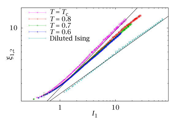
Figure 11.13: Plot of $\xi_{1,2}(t_{\mathrm{w}})$ as a function of $I_{1}(t_{\mathrm{w}})$ for our three subcritical spin-glass runs and for our run at $T=1.1\approx T_{\text{c}}$. We also include, as a comparison, the analogous plot for a $D=2$ site-diluted Ising model. We expect a behaviour $\xi_{1,2}^{2-\theta(0)}\propto I_{1}$, with a different $\theta(0)$ in each case. The diluted Ising is a coarsening system, so $\theta(0)=0$ and $\xi_{1,2}\propto I_{1}^{1/2}$. The critical simulation is well represented by $\theta(0)=1+\eta$ (full line, taking the anomalous dimension from [hasenbusch:08b]). On the other hand, the subcritical spin-glass simulations show an intermediate value of $\theta(0)$, different both from the critical and the coarsening predictions.

$T$	$N_{\text{samples}}$	$[\xi_{\text{min}},\xi_{\text{max}}]$	$z$	$\theta(0)$	$\chi^{2}_{\xi}$/d.o.f.	$\chi^{2}_{I_{1}}$/d.o.f.
$0.6$	96	$[3,10]$	14.06(25)	0.359(13)	41.7/82	49.0/82
$0.7$	768	$[4,10]$	11.64(15)	0.397(12)	40.1/58	60.4/58
$0.8$	96	$[3,10]$	9.42(15)	0.442(11)	17.1/63	12.2/63
$1.1$	32	$[3,10]$	6.86(16)	0.585(12)	18.7/46	26.1/46

Table 11.6: Computation of the replicon exponent $\theta(0)$ with non-equilibrium methods. For each temperature, we include the range of $\xi_{1,2}$ in which we computed the separate fits for $I_{1}$ and $\xi_{1,2}$ and the $\chi^{2}_{\text{d}}/\text{d.o.f.}$ for each fit. Notice that the fits for $\xi_{1,2}$ are the same ones reported in Table 10.1.

Recalling the integrals $I_{k}(t_{\mathrm{w}})$, defined in (10.22), and our choice of $\xi_{1,2}(t_{\mathrm{w}})$ for estimating the coherence length, we have

$$I_{1}(t_{\mathrm{w}})\propto[\xi_{1,2}(t_{\mathrm{w}})]^{2-\theta(0)}.$$ (11.53)

We have plotted $I_{1}$ against $\xi(t_{\mathrm{w}})$ in Figure 11.13 for $T=0.6,0.7,0.8,T_{\text{c}}$. We also include, as a comparison, the same plot for the $D=2$ site-diluted Ising model, a system that we know follows the $\theta(0)=0$ coarsening behaviour. From this plot we see that the value of $\theta(0)$ for our subcritical temperatures is clearly different both from the coarsening behaviour and from the critical value. On the other hand, the curve at $T=T_{\text{c}}$ seems to follow the expected $\theta(0)=1+\eta$ behaviour. Notice also that $\theta(0)$ is at least very similar for all the subcritical temperatures, in accordance with our theoretical expectation (but in clear contrast with the behaviour of the dynamic critical exponent $z$, which was inversely proportional to $T$).

In order to compute the actual value of $\theta(0)$ we could in principle fit $I_{1}$ to (11.53) as a function of $\xi_{1,2}$. Notice that these variables are highly correlated, which should reduce the statistical errors in $\theta(0)$. However, we would face the complicated problem of fitting strongly correlated data to a functional form $y=f(x)$ with errors in both the $x$ and $y$ coordinates. We faced quite the same difficulty when estimating the exponent $d$ measuring the decay of the thermoremanent magnetisation in Section 10.4 and we can adopt the same solution. In particular, we fit $I_{1}(t_{\mathrm{w}})$ to a power law,

$$I_{1}(t_{\mathrm{w}})=Bt_{\mathrm{w}}^{c}$$ (11.54)

and recall that $\xi_{1,2}(t_{\mathrm{w}})=At_{\mathrm{w}}^{1/z}$, Eq. (10.26). Therefore

$$\theta(0)=2-cz,$$ (11.55)

a relation that we can apply for each jackknife block.

The results of following this procedure are quoted in Table 11.6. As we can see, the values of $\theta(0)$ below $T_{\text{c}}$ are not actually compatible. However, the value at $T=0.8$ is probably affected by critical effects, while the values at $T=0.6,0.7$ are actually very close (see also Section B.3.3.1 for some technical issues with these fits). Therefore, we use the interval between the computations at $T=0.6$ and $T=0.7$ as our confidence interval for the replicon exponent,

$$\theta(0) =0.38(2), T<T_{\text{c}}.$$ (11.56)

This value is in good agreement with a previous (but much less precise) ground-state computation giving $$\theta(0)\approx 0.4 T=0 T=T_{\text{c}}$$ at  [marinari:01]. On the other hand, at we have

$$\theta(0) =0.585(12), T=T_{\text{c}}.$$ (11.57)

This value is a couple of standard deviations away from the estimate we quoted in (11.51). This difference is at the limit of statistical significance and could be due either to corrections to scaling or to a small cutoff error in our computations of the coherence length and $I_{1}$ (we have fewer samples at $T_{\text{c}}$, see Section B.3.3.1 for a discussion of this issue).

11.3.2 Equilibrium study

Let us now examine the scaling of the equilibrium connected correlations. We shall first carry out a study in real space, using the previously computed $\theta(0)$ as a starting point. Then, as in Section 10.8, we change into Fourier space, more convenient for a fully quantitative analysis.

11.3.2.1 Real space

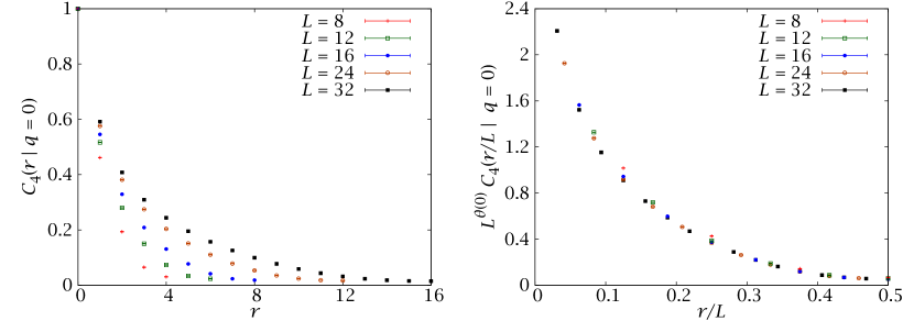
Figure 11.14: Spatial correlation function $C_{4}(r|q=0)$ at $T=0.703$. We show on the right panel a rescaled version using the replicon exponent $\theta(0)=0.38$ and the scaling variable $r/L$.

We first concentrate on $q=0$, the region where the droplet and RSB prediction are most different. Here, see Figure 11.14, the correlation function is seen to go to zero for large distances. Furthermore, in order for the droplet scaling as $r/L$ of (11.34) to work, we need to rescale our data by a factor $L^{\theta(0)}$, using our previously computed value of $\theta(0)=0.38(2)$.

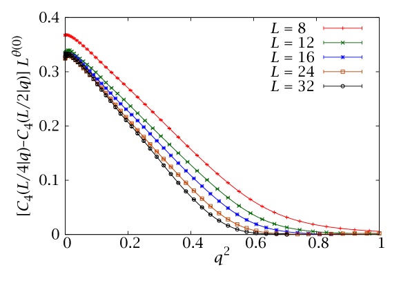
Figure 11.15: Subtracted correlation functions in units of $L^{-\theta(0)}$ as a function of $q$. We used $\theta(0)=0.38(2)$ from (11.56).

For $|q|>0$, in principle we have to compute explicitly the connected correlation $C_{4}(r|q)-q^{2}$. This subtraction is problematic for finite lattices [contucci:09], so instead we take care of the large-$r$ background by considering the differences

$$C_{4}(r=L/4|q)-C_{4}(r=L/2|q)\sim L^{-\theta(q)},$$ (11.58)

We see in Figure 11.15 that the above differences scale with $L^{-\theta(0)}$ in a finite $q$ range (approximately for $q^{2}<0.2$). This is a new piece of evidence in favour of the clustering property, that is, of the algebraic decay of connected correlations.

On the other hand, for $q^{2}=q_{\text{EA}}^{2}\approx 0.3$ the exponent is clearly larger than $\theta(0)$. The fact that the scaling with $\theta(0)$ holds for a finite range and that, in particular, there seems to be no discontinuity at $q=0$ suggests the following scenario

$$\theta(0\leq|q|<q_{\text{EA}})=\theta(0)<\theta(q_{\text{EA}}).$$ (11.59)

Therefore, we are in the conditions for the scaling law (11.49) to hold and we should have $\theta(0)=1/\hat{\nu}$. In fact, our results are

$$\theta(0) =0.38(2),$$ (11.60)

$$1/\hat{\nu} =0.39(5),$$ (11.61)

compatible with this expectation. We still lack, however, one final piece in the puzzle: the actual value of $\theta(q_{\text{EA}})$. We shall attempt to compute it in Fourier space in the next section.

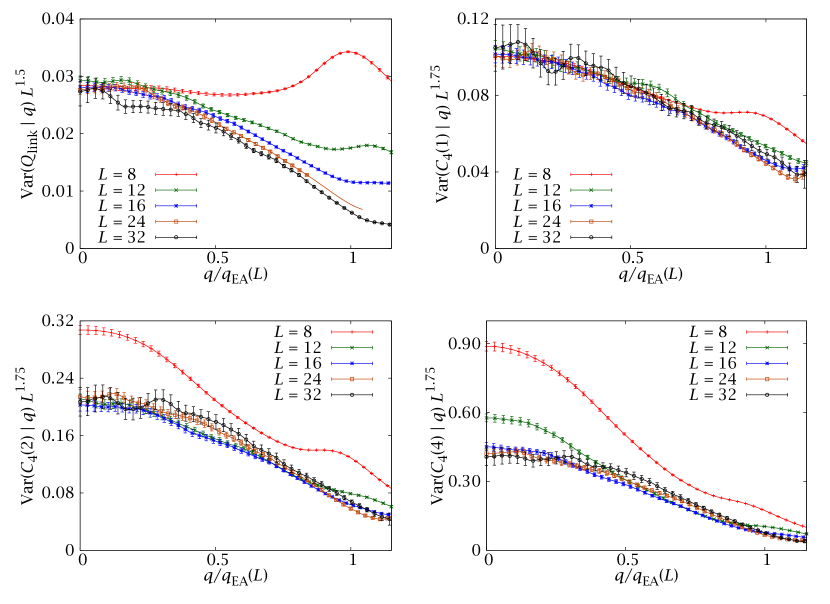
Figure 11.16: Conditional variance of the spatial correlation functions at $T=0.703$, which is seen to scale as $\sim L^{-1.75}$, faster than the $L^{-1.5}$ scaling of $\mathrm{Var}(Q_{\text{link}}|q)$.

Let us conclude the real-space study by examining the conditional variance of the correlation function. We shall write $\mathrm{Var}\bigl{(}C_{4}(r)|q\bigr{)}$ in an abuse of language ($C_{4}$ is already defined as an averaged quantity, not a random variable) that we hope will create no confusion. Notice that, while $\mathrm{E}(Q_{\text{link}}|q)=C_{4}(r=1|q)$ the variance $\mathrm{Var}(Q_{\text{link}}|q)$ is different than $\mathrm{Var}\bigl{(}C_{4}(1)|q\bigr{)}$. These variances are plotted in Figure 11.16, where they are seen to decrease with $L$ even faster than $\mathrm{Var}(Q_{\text{link}}|q)$.

11.3.2.2 Fourier space

$L$	$T=1.109$		$T=0.703$
	$F_{0}$		$F_{0}$	$F_{q_{\mathrm{EA}}}$
8	16.126(64)		19.46(18)	10.373(48)
12	40.59(18)		53.65(62)	25.79(15)
16	79.07(31)		112.5(13)	51.60(29)
24	204.05(83)		327.3(43)	134.54(80)
32	404.4(29)		699(23)	267.9(30)
$L_{\mathrm{min}}$	8		8	16
$\chi^{2}/\mathrm{dof}$	$0.90/3$		1.38/3	0.13/1
$\theta$	$0.638\,2(44)$		0.377(14)	0.611(16)[60]

Table 11.7: $F_{q=0}$ for our different system sizes and temperatures $T\!=\!1.109\!\approx\!T_{\mathrm{c}}$ and $T\!=\!0.703$. We report at the bottom power-law fits $F_{q}\!=\!A\ell^{D-\theta(q)}$ in the range $L\!\geq\!L_{\mathrm{min}}$. At $T\!=\!0.703$ we also consider $F_{q}$ at $q\!=\!0.523\!\approx\!q_{\mathrm{EA}}$. The second error bar, in square brackets, accounts for the uncertainty induced by the determination of $q_{\mathrm{EA}}$ (a larger $q_{\text{EA}}$ produces a larger $\theta$).

In the previous section we saw that the equilibrium spatial correlations scaled well at $q=0$ with the $\theta(0)$ computed out of equilibrium and that, indeed, this same exponent seemed to rule the scaling for a finite $q$ range.

Here we want to make a more quantitative study, using the correlations in Fourier space (more convenient at $q\neq 0$, since they do not require a subtraction). In particular, we shall obtain independent estimates of $\theta(0)$ and $\theta(q_{\text{EA}})$ and test the hypothesis of constant $\theta(q)$ in the range $0\leq q<q_{\text{EA}}$.

To this end, let us recall definition (10.65) and perform fits to

$$F_{q}=A_{q}\ell^{D-\theta(q)},$$ (11.62)

where $\ell$ was defined in (11.26). We have done this for $q=0$ and $q=q_{\text{EA}}$ at $T=0.703$ in Table 11.7. The scaling at $q=0$ is very good and we obtain

$$\theta(0)=0.377(14),$$ (11.63)

in excellent agreement with our non-equilibrium estimate (11.56). For $q=q_{\text{EA}}$, however, we need to restrict our fitting range to $L\geq 16$. Furthermore, the uncertainty in $q_{\text{EA}}=0.52(3)$ induces a systematic error, which we denote with square brackets. Our final estimate is

$$\theta(q_{\text{EA}})=0.611(16)[60].$$ (11.64)

This estimate is compatible with the scaling law $\theta(q_{\text{EA}})=2/\hat{\nu}$ —recall that $1/\hat{\nu}=0.39(5)$.

For the sake of completeness, and as a check of our procedure, we have also computed $\theta(0)$ at $T_{\text{c}}$. Our result, $\theta(0)=0.638(4)$, is very different from the value at $T=0.703$ and compatible with the best result in the literature [hasenbusch:08b], $\theta(0)=0.625(10)$ (our error bar is deceptively small, because we have not taken scaling corrections into account, unlike [hasenbusch:08b]).

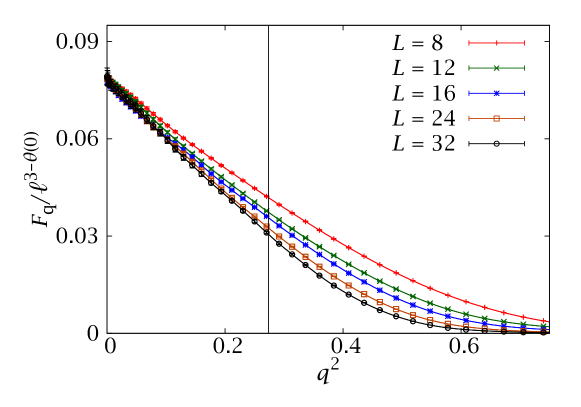
Figure 11.17: Plot of $F_{q}$ at $T=0.703$ in units of $\ell^{D-\theta(0)}$. As in the real-space representation of Figure 11.15, we can see a good scaling for a finite range in $q$. The vertical line marks our estimate of $q_{\text{EA}}^{2}$.

Finally, let us test the hypothesis of constant $\theta(q)$ for $|q|<q_{\text{EA}}$. To this end, we show in Figure 11.17 the analogous plot to Figure 11.15 in Fourier space. Not only do we see a good scaling with $\theta(0)$ for a finite range, as in Figure 11.15, but now in our Fourier-space representation each of the curves is linear in $q^{2}$ below $q_{\text{EA}}^{2}$. Therefore, we have performed the following fit

$$F_{q}-F_{0}=-a_{2}q^{2}+a_{4}q^{4}.$$ (11.65)

Notice that, since the data at different $q$ are correlated, subtracting the $q=0$ value yields a significant error reduction. The quadratic term is only included to control systematic effects in the computation of $a_{2}$ (and it probably causes us to overestimate errors). We report the resulting vales of $a_{2}$ in Table 11.8.

$L$	$a_{2}$
8	35.6(18)
12	110.4(58)
16	254(12)
24	816(40)
32	1823(216)

Table 11.8: Coefficient $a_{2}$ in a fit to (11.65) for for $q^{2}<0.5$ at $T=0.703$.

Now, in the case of discontinuous $\theta(q)$, one would expect a behaviour

$$a_{2}(L)=b\ell^{c},$$ (11.66)

with $c>D-\theta(0)$. If we perform this fit from the data in Table 11.8, we obtain $c=2.91(6)$, with $\chi^{2}/\text{d.o.f.}=0.08/3$. Yet, the extremely small $\chi^{2}$ is an indication that we have probably overestimated the errors in $a_{2}$. Therefore, let us take the value of $c$ seriously and consider the scaling of $F_{q_{*}}$ with $q_{*}=0.1<q_{\text{EA}}$. Then, in order for the would-be different scaling at $q_{*}$ to be noticeable, we need a lattice size large enough so that

$$F_{0}-F_{q}\approx a_{2}q_{*}^{2}\sim F_{0}.$$ (11.67)

The reader can check that this results in an enormous $L\sim 3\times 10^{6}$. Therefore, we do not find any numerical evidence in favour of the perturbative prediction of a discontinuity at $q=0$.

Let us go back our favoured scenario of constant $\theta(q)$ in $|q|<q_{\text{EA}}$. Then, the linear behaviour of $F_{q}$ with $q^{2}$ suggests a scaling

$$a_{2}(L)=e\ell^{D-\theta(0)}(1-d\ell^{\theta(0)-\theta(q_{\text{EA}})}).$$ (11.68)

In addition, in this hypothesis of constant $\theta(q)$ we have $\theta(0)=1/\hat{\nu}=\theta(q_{\text{EA}})/2$ from (11.37) and (11.49). Therefore, we can write

$$a_{2}(L)=e\ell^{D-\theta(0)}(1-d\ell^{-\theta(0)}).$$ (11.69)

Fitting the data in Table 11.8 to this expression, fixing $\theta(0)=0.38(2)$ and varying only the amplitudes, we obtain an excellent $\chi^{2}/\text{d.o.f.}=0.35/3$. Therefore, the simplest scenario consistent with the data is

$$\theta(|q|<q_{\text{EA}}) =\theta(0)=1/\hat{\nu}=0.38(2),$$ (11.70)

$$\theta(q_{\text{EA}}) =2\theta(0).$$ (11.71)

CHAPTER XII   Conclusions and outlook

In this dissertation we have explored two main themes in the context of the statistical mechanics of disordered systems,

1. It is worthwhile (and feasible) to consider a statistical ensemble tailored to the problem at hand, both from the point of view of achieving thermalisation and in order to obtain the maximum amount of physical information about the system.

2. When working with disordered systems, one cannot help dealing with non-equilibrium phenomena. In this sense, a quantitative relation between the equilibrium phase and the non-equilibrium evolution can, and should, be established.

We took a Monte Carlo simulation approach to both issues, carrying out simulations in a variety of computing systems (conventional computing clusters, supercomputing facilities and grid resources) for a combined total of several millions of CPU hours. In addition, we analysed the data from about one year of non-stop production of Janus, a special-purpose machine equivalent to many thousands of conventional computers.

In regards to the first point we introduced the Tethered Monte Carlo method, a general formalism to reconstruct the Helmholtz effective potential associated to an arbitrary reaction coordinate. The method consists in performing individual Monte Carlo simulations at fixed values of the reaction coordinate, which are then combined to construct the Helmholtz potential from a fluctuation-dissipation formalism. By choosing an appropriate reaction coordinate (i.e., one that labels the different relevant metastable states) it is possible to use this method to obtain a comprehensive picture of the system’s physics.

We demonstrated that this approach is indeed workable in physically relevant situations by tackling a classic ‘hard’ problem in the field of disordered systems: the phase transition of the diluted antiferromagnet in a field. We found that the tethered approach unlocked much information that remains hidden to a traditional method and we were able to obtain a comprehensive and consistent picture of the critical behaviour in this model.

We explored our second point, the statics-dynamics relation, in the field of spin glasses. There we analysed large-scale simulations performed on Janus. These were carried out both in and out of equilibrium and in both cases constituted a jump of several orders of magnitude with respect to the state of the art. We were able to use these high-quality data, combined with some novel analysis techniques, to establish a quantitative statics-dynamics equivalence and to determine the nature of the spin-glass phase up to the experimental scale.

In the following subsections we detail our conclusions and outlook for each of our three lines: Tethered Monte Carlo, the DAFF and the Edwards-Anderson spin glass.

12.1  The Tethered Monte Carlo method

We started by demonstrating our Tethered Monte Carlo method in the context of Ising ferromagnets. In this comparatively simple problem we found that our formalism, coupled to a local update algorithm, was able to reconstruct the effective potential without critical slowing down. We then showed that the method can be combined with sophisticated update schemes (cluster algorithms), in which case the critical slowing down disappeared even for non-magnetic observables.

We then applied Tethered Monte Carlo to a system with a rugged free-energy landscape: the DAFF (see below for the physical results). We found that the method was able to eliminate the exponential slowing down caused by the free-energy barriers associated to our reaction coordinates (the magnetisation and staggered magnetisation).

Thus, we were able to thermalise safely much larger systems that are possible with conventional methods, such as parallel tempering in the canonical ensemble. However, for our largest systems we started to see metastable behaviour caused by new free-energy barriers. In this sense, the onset of exponential slowing down was delayed, rather than outright eliminated.

Dealing with these new free-energy barriers will probably require the introduction of additional reaction coordinates, capable of a further classification of metastable states. Our method is in principle equipped to carry out this plan, but a practical implementation requires some work.

A different avenue for further work with Tethered Monte Carlo is extending its application to new systems. One interesting possibility is the study of the condensation transition [biskup:02, binder:03, macdowell:04, nussbaumer:06, nussbaumer:08], which can be modelled with Ising systems. We finally note that the tethered formalism has already been applied to the study of hard-spheres crystallisation [fernandez:11].

12.2  The diluted antiferromagnet in a field

The use of the tethered formalism allowed us to obtain a consistent picture of the critical behaviour in the DAFF. We obtained clear evidence in favour of the second-order nature of the transition and computed the three independent critical exponents. In particular, we obtained a precise determination, $\theta=1.469(20)$, for the elusive hyperscaling violations exponent. We also observed a clear divergence of the specific heat, in accordance with experimental work.

Still, there is much work still to do. In particular, our data for the $\nu$ critical exponent was affected by finite-size effects. Also, even if we determined that the specific-heat exponent $\alpha$ is positive, we could not estimate its precise value very precisely. To this end, the simulation of even larger systems would be required.

Finally, it would be very interesting to achieve a closer connection to experimental work. The obvious contact point would be obtaining a precise numerical determination of the scattering line shape, which is the basic quantity explored in experiments to characterise the critical behaviour. Our methods are well suited to carry out this programme in the future.

12.3  The Edwards-Anderson spin glass

We studied the $D=3$ Edwards-Anderson spin glass in and out of equilibrium and were able to establish a time-length dictionary, relating the equilibrium phase of a system of size $L$ and the non-equilibrium state at time $t_{\mathrm{w}}$ of a system in the thermodynamical limit. In particular, we reached the conclusion that the equilibrium phase of a system of size $L\sim 100$, and not the thermodynamical limit, is the relevant one for understanding experimental work on spin glasses.

We later took this quantitative statics-dynamics connection one step further by establishing a finite-time scaling framework. This last result, in which dynamical heterogeneity played a major role, has implications for experimental work.

The above studies were carried out in a neutral formalism, without assuming the validity of any particular theory for the spin-glass phase. A more detailed analysis of the spin-glass phase showed clear evidence in favour of the RSB picture, at least for experimentally relevant scales. We based this conclusion on three main observations: (i) non-triviality of the spin overlap, (ii) overlap equivalence and (iii) the existence of a non-zero replicon exponent.

When trying to decide which is the relevant theory in the thermodynamical limit (equivalent to the limit of infinite experimental time), we found that our data still supported the RSB picture, but here our results are not as conclusive (in principle, there can always appear a change of regime for much larger sizes or much longer times, even if we see no trace of it with our data).

There are several promising avenues for future work in this field. First, deciding in favour of RSB for the nature of the spin-glass phase does not automatically grant one full knowledge of its characteristics. Much work is needed in order to work out some very important details, such as the nature of temperature chaos.

Perhaps the most interesting prospect for future work is trying to reproduce, as realistically as possible, an actual spin-glass experiment. Our non-equilibrium simulations only considered the simplest protocol of isothermal aging, but many interesting effects (memory, rejuvenation, etc.) can only be observed by varying the temperature. In this sense, our current simulations were limited by the onset of finite-size effects. Indeed, for temperatures close to the critical point, our simulated size $L=80$ is not large enough to be representative of the non-equilibrium physics for experimentally relevant times, since the coherence length grows too quickly. Let us stress that although this effect is restricted to the vicinity of the critical temperature, any experimental cooling protocol should expend a time close to $T_{\text{c}}$ which is very long in the microscopic scale.

Simulating even larger lattices is, therefore, a must if one wants to reproduce sophisticated experimental protocols. We are very optimistic in this sense: we are already testing a code that allows us to simulate lattices of size $L=256$ and we also have funding for Janus II, which will not only allow us to simulate even larger systems, but also to probe longer times, taking us fully into the experimental regime.

Appendix A Thermalisation in Monte Carlo simulations

This appendix is intended as a reference on thermalisation in Monte Carlo simulations, providing some definitions that are used throughout this thesis. Most of the definitions are standard, but subsection A.3.1 contains some methods developed in part during this thesis.

A.1  Markov chain Monte Carlo

Let us begin by recalling some definitions and results relevant to the theory of dynamic Monte Carlo methods (this is not meant to be a rigorous or self-contained account, just a quick reference, cf. [sokal:97, rubinstein:07]). In general, we are interested in extracting configurations from some probability distribution $p(\{s_{\boldsymbol{x}}\})$, often of the kind $p(\{s_{\boldsymbol{x}}\})\propto\mathrm{e}^{-\beta E(\{s_{\boldsymbol{x}}\})}$. In order to simplify the notation, we denote the system configuration by a single random variable $X$ and our target probability distribution by $P_{x}=\mathcal{P}(X=x)$.

Then we define our Monte Carlo method as a random walk in configuration space, that is, a sequence $X_{t}$ of random variables. The first one —the starting configuration— will follow some simple probability distribution $P^{(0)}_{x}$ (completely random spins, for instance). We need the random walk to reach a stationary state such that $\lim_{t\to\infty}P^{(t)}_{x}=P_{x}$.

We consider a Markov chain: the probability distribution of $X_{t+1}$ depends only on $X_{t}$ and not on the whole previous history. Then, we can specify the whole process by giving the initial distribution $P^{(0)}_{x}$ and a transition matrix $U_{xy}$. The latter is defined as

$$U_{xy}=\mathcal{P}(X_{t+1}=y|X_{t}=x),$$ (a.1)

that is, the probability that the system will be in the configuration $y$ at time $t+1$ if it was at $x$ at time $t$. Of course, we can iterate this definition

$$[U^{n}]_{xy}=\mathcal{P}(X_{t+n}=y|X_{t}=x).$$ (a.2)

The objective is that, no matter the initial distribution $P^{(0)}_{x}$, after a sufficiently long number of iterations we obtain configurations distributed according to $P_{x}$. In other words

$$\lim_{n\to\infty}[U^{n}]_{xy}=P_{x}.$$ (a.3)

We need two ingredients for this

• First, we need our method to be capable of exploring the whole configuration space. To this end, we require the transition matrix to be irreducible: for all $x,y$ there exists an $n$ such that $[U^{n}]_{xy}>0$.

• Naively, we could think of requiring that, once we have reached the stationary distribution $P_{x}$, the Markov process should lose all sense of direction and be reversible. We should not be able to tell if it is running backwards or forwards. That is

  $$P_{x}U_{xy}=P_{y}U_{yx}.$$ (a.4)

  This is called the detailed balance condition. Actually, it turns out that this is too restrictive. We only need that the stationary distribution of the Markov chain correspond to $P_{x}$, that is

  $$P_{y}=\sum_{x}P_{x}U_{xy}.$$ (a.5)

  This is the balance condition.

If $U_{xy}$ satisfies these two conditions, then (a.3) can be proved and we have a legitimate Monte Carlo method. Notice that the balance condition is easier to check than it seems, since it does not depend on the normalisation of the $P_{x}$ (typically given by the unknown partition function $Z$).

Perhaps the easiest example of Monte Carlo dynamics is the heat bath. Let us consider the update of a single Ising spin at site ${\boldsymbol{x}}$, $s_{\boldsymbol{x}}\to s_{\boldsymbol{x}}^{\prime}$, where all the remaining spins in the lattice are kept fixed. Then, we consider the following update probability

$$\mathcal{P}(X_{t+1}=\{s^{\prime}\}|X_{t}=\{s\})=\frac{\mathrm{e}^{-\beta E(\{s^{\prime}\})}}{\sum_{s^{\prime\prime}_{\boldsymbol{x}}=\pm 1}\mathrm{e}^{-\beta E(\{s^{\prime\prime}\})}},$$ (a.6)

Notice that all the terms in the energy that do not involve site ${\boldsymbol{x}}$ factor out. Therefore, it is obvious that the update of a single spin satisfies the detailed balance condition. In order to define a full Monte Carlo method we need to update all the spins. We can do this by randomly choosing one spin each time and defining each Monte Carlo step as $N$ spin updates (so that each spin in the lattice is updated once, on average). In this case the whole transition matrix would also satisfy detailed balance. We can also consider a scheme where we run through the lattice sequentially, visiting all the sites in order. In this case, the process would clearly not be reversible, and the transition matrix would only satisfy balance.

A.2  The autocorrelation times

As a general rule, the thermalisation of a Monte Carlo simulation (i.e., how long it takes to reach the stationary distribution) should be assessed through the temporal autocorrelation functions [sokal:97]. Let $O$ be an observable, defined as always as a real-valued function on the configuration space, and assume we have equilibrated the system for a very long time, so we have reached the stationary regime. Then, we consider the equilibrium (stationary) evolution $O(t)$ and define the equilibrium autocorrelation functions

$$C_{O}(t)=\bigl{\langle}[O(0)-\langle O\rangle][O(t)-\langle O\rangle]\bigr{\rangle},\qquad\rho_{O}(t)=\frac{C_{O}(t)}{C_{O}(0)}\ .$$ (a.7)

The angle brackets here denote any kind of thermal average (e.g., canonical or tethered). The autocorrelation function decays as an exponential for long times,

$$\rho_{O}(t)\xrightarrow{\ \ t\to\infty\ \ }A\exp[-t/\tau].$$ (a.8)

This asymptotic behaviour suggests the definition of the exponential autocorrelation time,

$$\tau_{\text{exp},O} =\lim_{t\to\infty}\sup\frac{t}{-\log|\rho_{O}(t)|},$$ (a.9)

$$\tau_{\text{exp}} =\sup_{O}\tau_{\text{exp},O}.$$ (a.10)

In general, we express the autocorrelation as a sum of exponentials

$$\rho_{O}(t)=\sum_{i}A_{i}\mathrm{e}^{-t/\tau_{i}}.$$ (a.11)

The exponential time, then, is the largest of the $\tau_{i}$ and characterises the relaxation time of a certain observable. Actually, barring symmetry considerations, the exponential time is the same for all observables.

Another useful concept is that of integrated autocorrelation time

$$\tau_{\text{int},O}=\frac{1}{2}+\sum_{t=1}^{\infty}\rho_{O}(t),$$ (a.12)

The integrated time indicates the minimum time difference so that two measurements of some observable $O$ can be considered independent (i.e., uncorrelated). In particular, if $\mathrm{Var}(O)$ is the variance of a single measurement of $O$ (after we have reached equilibrium) and we average over $\mathcal{N}$ successive such measurements, the resulting variance is

$$\mathrm{Var}\bigl{(}O^{(\mathcal{N})}\bigr{)}=\frac{\mathrm{Var}(O)}{\mathcal{N}/(2\tau_{\text{int},O})},$$ (a.13)

as opposed to the value $\mathrm{Var}(O)/\mathcal{N}$ that we would obtain for $\mathcal{N}$ statistically independent measurements.

The integrated time is less useful as a measure of thermalisation than the exponential. In fact, notwithstanding the previous discussion, the determination of $\tau_{\text{int},O}$ is not even always needed to estimate statistical errors (see Appendix B). It has, however, the considerable advantage of being much easier to measure safely. Notice as well that, if the decomposition (a.11) contains a single exponential, $\tau_{\text{exp},O}=\tau_{\text{int},O}$, This approximation can often be employed. Alternatively, if we do not take measurements for every single MCS or, better, if we make bins of consecutive measurements, we can neutralise the faster modes in (a.11) and approach the single-exponential limit. By ‘binning’ we understand averaging groups of $n$ consecutive measurements. In this case, all the components with $\tau_{i}\ll n$ dissappear. The same approach is taken in a different context, that of random variables strongly correlated in space, close to a critical point (Kadanoff-Wilson blocks).

A.2.1 Some computational recipes

For a large-scale MC simulation, where we have to handle very long time series (millions of time steps even after the binning procedure mentioned above), the computation of $\rho_{O}(t)$ can be time-consuming. Indeed, a naive implementation of definition (a.7) requires $\mathcal{O}(\mathcal{N}^{2})$ operations.

We can do better. For simplicity, and without loss of generality, let us consider an observable such that $\langle O\rangle=0$, for which we take $\mathcal{N}$ measurements $O(t)$, $t=0,\ldots,\mathcal{N}-1$. We also assume all this measurements have already been taken in the equilibrium regime (i.e., we have discarded a sufficient number of measurements for thermalisation). Then we could estimate $C_{O}$ as

$$[C_{O}(t)]=\frac{1}{\mathcal{N}-t}\sum_{s=0}^{\mathcal{N}-1-t}O(s)O(s+t).$$ (a.14)

Let us define

$$S_{O}(t)=(\mathcal{N}-t)C_{O}(t)$$ (a.15)

and

$$O^{\prime}(t)=\begin{cases}O(t),&0\leq t<\mathcal{N},\\ 0,&\mathcal{N}\leq t<2\mathcal{N},\end{cases}$$ (a.16)

and we consider $O^{\prime}(t)$ to be extended periodically.

Then we can write our numerical estimate for the unnormalised correlation of $O^{\prime}$ as

$$[S_{O^{\prime}}(t)]=\sum_{s=0}^{2\mathcal{N}-1}O^{\prime}(s)O^{\prime}(s+t)$$ (a.17)

Notice that

$$[S_{O^{\prime}}(t)]=[S_{O}(t)].$$ (a.18)

Now consider the Fourier transform of $S_{O^{\prime}}(t)$,

$$[\hat{S}_{O^{\prime}}(q)] =\sum_{t=0}^{2\mathcal{N}-1}\sum_{s=0}^{2\mathcal{N}-1}O^{\prime}(s)O^{\prime}(s+t)\mathrm{e}^{-\mathrm{i}qt}$$ (a.19)

Notice that, since we are summing $$t s+t\to t^{\prime}$$ over a whole period of the function, we can change in the second sum

$$[\hat{S}_{O^{\prime}}(q)] =\sum_{s=0}^{2\mathcal{N}-1}O^{\prime}(s)\sum_{t^{\prime}=0}^{2\mathcal{N}-1}O^{\prime}(t^{\prime})\mathrm{e}^{\mathrm{i}qs}\mathrm{e}^{-\mathrm{i}qt^{\prime}}$$ (a.20)

$$=\biggl{(}\sum_{s=0}^{2\mathcal{N}-1}O^{\prime}(s)\mathrm{e}^{\mathrm{i}qs}\biggr{)}\biggl{(}\sum_{t^{\prime}=0}^{2\mathcal{N}-1}O^{\prime}(t^{\prime})\mathrm{e}^{-\mathrm{i}qt^{\prime}}\biggr{)}=|\hat{O}(q)|^{2}.$$ (a.21)

That is, the Fourier transform of the autocorrelation is equal to the modulus of the Fourier transform of $O^{\prime}$ (we have needed a periodic $O^{\prime}$ to get this result). This is the Wiener-Khinchin theorem.

Therefore, we can obtain $S_{O^{\prime}}(t)=S_{O}(t)=(\mathcal{N}-t)C_{O}(t)$ by computing the Fourier transform of $O(t)$, evaluating its complex modulus and then computing the inverse Fourier transform of $|\hat{O}(q)|^{2}$. It may seem that we have gained nothing. However, the computation of discrete Fourier transforms, seemingly an $\mathcal{O}(\mathcal{N}^{2})$ task, can actually be done in $\mathcal{O}(\mathcal{N}\log\mathcal{N})$ operations using the Fast Fourier Transform algorithm (see, e.g., [press:92]). In the work reported herein we have always followed this method to evaluate temporal autocorrelation functions. We use the FFTW implementation reported in [frigo:05].

Notice that an analogous method can be followed to evaluate spatial correlations, as we will have ample occasion to do (especially in Part IV). In this case, even if the functions are three-dimensional, the procedure is even simpler, as the periodic boundary conditions are already built in. Therefore, we do not have to pad our observables with zeros, as in (a.16).

Once we have computed the $\rho_{O}(t)$ we need to estimate the autocorrelation times. For the exponential ones our only recourse is a fit to one or more exponential modes (see below). The integrated time must, in principle, be computed from the sum of our numerical estimate $[\rho_{O}(t)]$ extended to all our values of $t$. However, as is clear from our definition (a.14), the final times have much smaller statistics, so their contribution is nothing but a white noise. Therefore, $\tau_{\text{int},O}$ is best evaluated using a self-consistent window [sokal:97]

$$\tau_{\text{int},O}=\frac{1}{2}+\sum_{t=1}^{\varLambda}[\rho_{O}(t)],$$ (a.22)

where $\varLambda$ is chosen as $\varLambda=W\tau_{\text{int},O}$, with $W$ a tunable parameter ($W=6$ works well).

A.3  Thermalisation in disordered systems

The safe computation of the autocorrelation times described in the previous section requires a simulation time orders of magnitude larger than $\tau_{\text{exp}}$. This is not a problem when simulating ordered systems, because extending the simulation reduces the statistical error of the final results. With disordered systems, however, the main source of statistical error is the sample-to-sample fluctuation. Reducing the thermal error for each sample beyond a certain, easily reachable, threshold is useless.

Therefore, given a fixed computational budget, we would like to simulate each sample for the shortest possible time that ensures thermalisation. Since so short a run time does not permit a computation of the $\tau_{O}$ for physical observables, researchers have traditionally employed less rigorous methods to check thermalisation.

In general, the typical method is to study the time evolution of the disorder-averaged physical observables. In particular, one of the most widespread practical recipes is the so-called $\log_{2}$-binning. One divides the simulation time $\mathcal{N}$ in logarithmic intervals $\mathcal{I}_{n}$:

$$\mathcal{I}_{n}=(2^{-n+1}\mathcal{N},\ 2^{-n}\mathcal{N}],$$ (a.23)

Notice that with this definition time decreases with increasing $n$, so $\mathcal{I}_{0}$ corresponds to the second half of the run, $\mathcal{I}_{1}$ to the second quarter, etc. Then, one evaluates the thermal average for each sample and the disorder average, for each of the time intervals. If the last few $\mathcal{I}_{n}$ show no evolution, the simulations are considered to be thermalised.

This procedure is not optimal, because in many situations the thermalisation time is wildly dependent on the sample (see Figures 8.6 and 8.6 for the DAFF or Figures e.1 and e.2 for the Edwards-Anderson spin glass). Thus, if we choose a simulation time that would thermalise even the slowest samples, we will spend most of our time extending already well thermalised runs for no benefit. Worse, a stationary average over many samples may hide the fact that a few samples are still quite far from equilibrium (the thermalisation time can vary along several orders of magnitude from one sample to another).

One could toughen the $\log_{2}$-binning test by taking the correlations into account [fernandez:07]. Indeed, since the samples considered for each $\mathcal{I}_{n}$ are always the same, the difference between the resulting averages (even assuming complete temporal decorrelation) will typically be much smaller than their statistical errors. This is because, as we said earlier, the thermal fluctuations account for an almost negligible part of the total statistical error. We can take this into account by computing for each sample the differences between the average for $\mathcal{I}_{0}$ and each of the $\mathcal{I}_{n}$ and considering the evolution of these correlated differences, which have a much smaller error (see Figure 8.9). To be sure, this is a more stringent test, but ultimately an unphysical one (because it considers much smaller errors than those of the physical results). Furthermore, it does not address the important problem of efficiency.

In the next section we shall see how we can provide a more rigorous method, taking advantage of the parallel tempering algorithm used to accelerate the thermalisation.

A.3.1 Parallel tempering

Parallel tempering [hukushima:96, marinari:98b] is one of the most common methods to accelerate thermalisation. Its motivation is the rugged free-energy landscape picture described in the General Introduction. Let us consider a system described in the canonical ensemble by the following partition function

$$Z(\beta)=\sum_{\{s_{\boldsymbol{x}}\}}\mathrm{e}^{-\beta E}.$$ (a.24)

At a physically interesting low temperature the system is trapped in deep free-energy valleys, with extremely long escape times. At a higher temperature, however, the energy fluctuations are enough to overcome these barriers quickly.

We can take advantage of this by simulating ${\mathcal{N}}_{T}$ copies of the system (in our case, ${\mathcal{N}}_{T}$ starting configurations with the same disorder realisation). Each copy starts the simulation at a different temperature, with $T_{1}<T_{2}<\ldots<T_{{\mathcal{N}}_{T}}$. We assume that $T_{1}$ is such that our chosen Monte Carlo dynamics would need an impossibly long time to thermalise the system, while $T_{{\mathcal{N}}_{T}}$ is high enough for the same dynamics to achieve thermalisation very quickly. After updating each copy independently for one or more MCS we perform the parallel tempering update.

Then, we consider a configuration space with ${\mathcal{N}}_{T}(V+1)$ degrees of freedom, $\{T^{(i)},\{s_{\boldsymbol{x}}^{(i)}\}\}$. The temperature associated to copy $i$ of the system can change, but the ensemble of temperatures $\{\beta^{(i)}\}$ must always be a permutation of

$$\{\beta_{1},\ldots,\beta_{{\mathcal{N}}_{T}}\}=\{1/T_{1},\ldots,1/T_{{\mathcal{N}}_{T}}\}.$$ (a.25)

Now, the partition function of the whole ensemble of systems is

$$Z_{{\mathcal{N}}_{T}}=\frac{1}{{\mathcal{N}}_{T}!}\prod_{i=1}^{{\mathcal{N}}_{T}}Z(\beta^{(i)}).$$ (a.26)

We can compute the marginal distributions for the $\beta^{(i)}$. Summing over the spins, we find that the marginal probability density of the temperature configuration $\{\beta^{(i)}\}$ is uniform,

$$p(\{\beta^{(i)}\})=1/({\mathcal{N}}_{T}!).$$ (a.27)

Moreover, the marginal probability for a single temperature is also uniform,

$$p(\beta^{(i)})=1/{\mathcal{N}}_{T}.$$ (a.28)

The partition function (a.26) allows us to consider a Monte Carlo dynamics where we simply try to exchange copies $i$ and $j$ of the system, initially at neighbouring temperatures $T_{k}$ and $T_{k+1}$,

$$\begin{split}\{\beta^{(i)}=\beta_{k},\{s_{\boldsymbol{x}}^{(i)}\}\}&\times\{\beta^{(j)}=\beta_{k+1},\{s_{\boldsymbol{x}}^{(j)}\}\}\ \longrightarrow\\ &\longrightarrow\ \{\beta^{(i)}=\beta_{k+1},\{s_{\boldsymbol{x}}^{(i)}\}\}\times\{\beta^{(j)}=\beta_{k},\{s_{\boldsymbol{x}}^{(j)}\}\}.\end{split}$$ (a.29)

The Metropolis acceptance probability (see Section 3.2) for this dynamics is

$$\mathcal{P}=\min\{1,\omega_{\text{new}}/\omega_{\text{old}}\}=\min\bigl{\{}1,\exp\bigl{[}-(\beta_{k+1}-\beta_{k})(E^{(j)}-E^{(i)})\bigr{]}\bigr{\}}.$$ (a.30)

In order for this dynamics to be irreducible, a full parallel temperature update consists in attempting one exchange per temperature, going sequentially from the lowest to the highest (so one configuration can actually jump several temperatures in a single update).

This way, the temperature of each copy performs a random walk in temperature space. Once the system reaches a high enough temperature, a few MCS are enough to make it cross the free-energy barriers so when it eventually returns to its original temperature it has been decorrelated from the starting configuration.

Notice that for this algorithm to work, we need to choose the participating temperatures close enough for their energy histograms to overlap, so the acceptance probability (a.30) is high enough.

A.3.2 The temperature random walk

In equilibrium, each copy should spend the same time at each temperature (recall (a.27)), so studying the temperature random walk can give information about the thermalisation. In particular, several round trips from lowest to highest temperature are needed for a system to be considered thermalised.

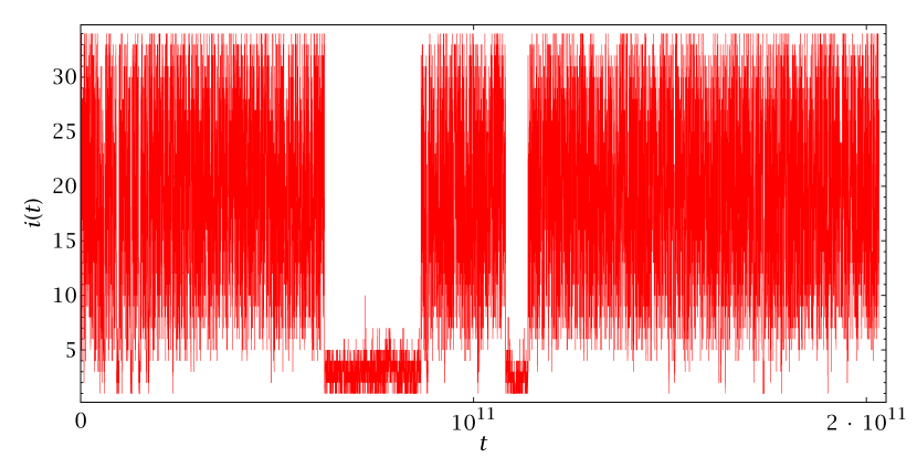
Figure a.1: Temperature random walk of a single configuration in one of our spin-glass simulations of Appendix E. We plot the temperature index $i(t)$ against the time measured in heat bath updates. The critical temperature corresponds to $i_{\text{c}}=17$ (in the middle of the range).

We can promote this idea to a fully quantitative and physically meaningful level. Let us assume that our range of temperatures crosses the critical point and let us define $i_{\text{c}}$ such that

$$T_{i_{\text{c}}-1}<T_{\text{c}}<T_{i_{\text{c}}}.$$ (a.31)

Now, for one of the ${\mathcal{N}}_{T}$ copies of the system, we consider its temperature random walk mapped to the range of the temperature index $i(t)\in\{1,\ldots,{\mathcal{N}}_{T}\}$. Figure a.1 shows one example, taken from our spin-glass simulations. Notice that the random walk is clearly not Markovian, as evinced by the long plateaux, since the system retains for a long time a memory that it started in the high (or low) temperature phase.

Our goal is to construct a quantity that is both representative of the random walk and amenable to the computation of autocorrelation times described in the previous section. To this end, we consider a mapping $f(i)$ such that

$$f(i) \geq 0, \forall i\geq i_{\text{c}},$$ (a.32)

$$f(i) <0, \forall i<i_{\text{c}},$$ (a.33)

$$\sum_{i=1}^{{\mathcal{N}}_{T}}f(i) =0.$$ (a.34)

Recalling (a.28), we see that the last condition is just $\braket{f}=0$. It is also convenient that $f$ be monotonic. Generally, one chooses the temperatures so that $i_{\text{c}}$ is in the middle of the range, so a simple linear $f$ suffices.

Now we can compute the autocorrelation $C_{f}(t)$ with Eq. (a.14). Notice that $f$ has an advantage over the $C_{O}$ of the physical observables: we can average the correlations over the ${\mathcal{N}}_{T}$ copies in the parallel tempering. These are not, of course, completely independent (the most obvious constraint being that each must be at a different temperature), but still the averaged correlation has a much smaller variance. Furthermore, in the case of spin glasses one simulates several statistically independent replicas, which provide an additional averaging layer and allow an estimate of the statistical error.

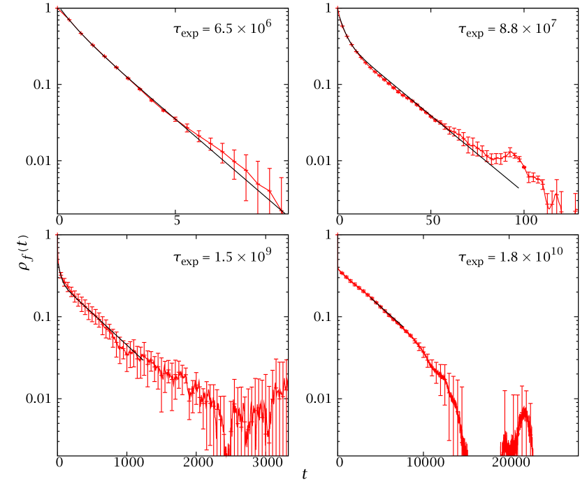
Figure a.2: Autocorrelation functions for some of our equilibrium spin-glass simulations of Appendix E, showing samples with $\tau_{\text{exp}}$ across several orders of magnitude, plotted against the simulation time in units of $10^{6}$ MCS. We have plotted the range $[0,6\tau_{\text{exp}}]$ and also show the result of the automated fitting procedure described in Section A.3.3. In order to avoid cluttering the graphs we have only plotted a few times (the actual correlation functions have many more points). In the last panel the correlation function has a strong downwards fluctuation. Our fitting code takes this into account by choosing a restricted range and fitting to a single exponential.

As explained in Section A.2, the thermalisation of the system is characterised by the exponential autocorrelation time. Recall that, barring symmetry considerations, the exponential time should be the same for all random variables in the simulation, including the physical observables. In general, the exponential autocorrelation time must be computed from a fit to an equation such as (a.11), with an appropriate number of exponential modes. This is not a problem for ordered systems simulations, where one can simply select the fitting range and functional form manually. When simulating disordered systems, however, one would have to do thousands of such fits, each with a different fitting range (in our study of the DAFF, for instance, we performed several hundred thousands independent parallel tempering simulations).

Clearly, an automated system must be found. The first step is making the $C_{f}(t)$ as simple as possible. In this respect we notice that the choice of $f$ should not modify the exponential autocorrelation time, but will affect the relative sizes of the $A_{i}$. Our criteria (a.32) and (a.33) hopefully select a family of functions that reduce the amplitude of the irrelevant fast modes. A second simplification is afforded by the sheer length of the simulations in practical cases. From a look at Tables 8.1 and e.2 we see that the runs can be as long as $10^{12}$ MCS. In this situation, averaging the $f\bigl{(}i(t)\bigr{)}$ over a large number of consecutive measurements implies no real information loss (as long as the bins are much smaller than $\tau_{\text{exp}}$). This binning procedure also has the welcome side effect of suppressing the fastest modes.

With these considerations in mind, in practice it turns out that the $\rho_{f}(t)$ can be adequately described by considering just two exponential modes. As an example of this, we have plotted in Figure a.2 several autocorrelation functions from our spin-glass simulations. The depicted correlation functions have been chosen randomly, with the only condition that they represent samples with very different exponential autocorrelation times.

A.3.3 Thermalisation protocol for parallel tempering simulations

We can summarise the previous discussion in the following three-step thermalisation procedure

1. Simulate for a minimum length of ${\mathcal{N}}^{\text{min}}$ MCS, chosen to be enough to thermalise most samples. Notice that most published parallel tempering studies stop here, assessing thermalisation only through the evolution of disorder-averaged observables.

2. Discard the first sixth of the measurements and compute the $\rho_{f}(t)$ from the remainder. Compute the integrated autocorrelation time with the self-consistent window method of Eq. (a.22), using $W=6$. Using this first estimate of the integrated time, we extend the simulation until ${\mathcal{N}}>A^{\text{int}}\tau_{\text{int}}$, always discarding the first sixth. This criterion was introduced in [fernandez:09b].

3. Now that the simulation is reasonably dimensioned, estimate $\tau_{\text{exp}}$ (typically of the same order of magnitude as $\tau_{\text{int}}$, but always bigger). Extend the simulations until ${\mathcal{N}}>A^{\text{exp}}\tau_{\text{exp}}$.

The actual thresholds $A^{\text{int}}$ and $A^{\text{exp}}$ are somewhat arbitrary and should be tuned to the system at hand (especially $A^{\text{int}}$, since the integrated time, unlike the exponential one, depends on the choice of $f$ and the frequency of its measurements).

We introduced the third step in this protocol for our spin-glass simulations in [janus:10], choosing $A^{\text{int}}=22$, $A^{\text{exp}}=12$ (see A.3.3.2 for our criteria for the DAFF). Notice that this implied performing non-linear fits with custom ranges for some $10^{4}$ autocorrelation functions. The first step was parameterising $\rho_{f}(t)$ by a double exponential decay (an assumption empirically justified by the shape of these correlation functions, cf. Figure a.2).

$$\rho_{f}(t)\simeq A_{1}\mathrm{e}^{-t/\tau_{1}}+A_{2}\mathrm{e}^{-t/\tau_{2}},\qquad\tau_{1}=\tau_{\text{exp}}>\tau_{2}.$$ (a.35)

The choice of fitting range of course depends on the values of the $\tau_{i}$, which vary across several orders of magnitude from one sample to another. However, notice that, if $A_{2}=0$, then $\tau_{\text{exp}}=\tau_{\text{int}}$. Therefore, $\tau_{\text{int}}$ is a good starting assumption for $\tau_{\text{exp}}$, so we took the following steps:

1. Perform a first fit to a single exponential in the range $[2\tau_{\text{int}},3\tau_{\text{int}}]$, yielding an amplitude $A$ and a time $\tau$.

2. Using $\tau_{1}=\tau$, $\tau_{2}=\tau/10$, $A_{1}=A$ and $A_{2}=1-A$ as a starting point, perform a non-linear fit to (a.35), with the fitting range $[\tau_{\text{int}}/10,10\tau_{\text{int}}]$.

In most cases we can stop here. Sometimes, however, the second fit fails —typically because one of the amplitudes is very small, so $\rho_{f}(t)$ is indistinguishable from a single exponential. This can be detected, and solved, in a number of ways:

1. One of the $A_{i}$ is $A_{i}\gg 1$, $\tau_{1}$ has an absurdly large value (indicating a fit to a short plateau in a noisy range) or the iterative fitting method breaks down. In these cases, a single exponential fits the data better. We perform a fit to a single exponential in the range $[5\tau_{\text{int}},10\tau_{\text{int}}]$.

2. One of the $A_{i}$ is negative, indicating an unphysical downwards fluctuation in the $\rho_{f}(t)$ for large times (cf. bottom-left panel of Figure a.2). We perform a fit to a single exponential in the reduced range $[2.5\tau_{\text{int}},3.5\tau_{\text{int}}]$.

A.3.3.1 Fail-safe mechanisms

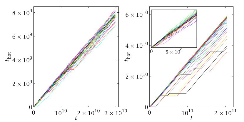
Figure a.3: Time spent above the critical temperature against total simulation time for two spin-glass samples. In each case we plot the ${\mathcal{N}}_{T}$ copies of the system. The left panel shows an ‘easy’ sample, where the random walk is relatively fluid and all configurations progress gradually. The right panel shows a ‘hard’ sample, where the configurations get trapped in local minima at low temperatures, producing long plateaux (notice the scales in both plots). In a very short run time (inset), only one of the copies of the second system would betray its hard character.

This automatic and fully quantitative procedure works for most samples, but there are some potential pitfalls that can lead to our underestimating $\tau_{\text{exp}}$. For instance, the exponential time may sometimes be much larger than $\tau_{\text{int}}$. In these situations, $A_{1}$ is very small and it is very difficult to fit the data properly. Therefore, if our fitting method detects $\tau_{\text{exp}}>10\tau_{\text{int}}$, we increase the measurement bins by a factor of $10$, making both $\tau_{\text{int}}$ and $A_{1}$ grow and easing the fitting procedure.

More generally, we have assumed that our $\rho_{f}(t)$ has been measured in equilibrium, or close to it (i.e., that our simulation is at least a couple of $\tau_{\text{exp}}$ long). In a very short run, however, some of the configurations may not even have had time to visit the relevant minima, and get trapped in them, producing a misleadingly fluid random walk. In particular, this happens when some of the copies have not crossed the critical temperature in the parallel tempering dynamics. To prevent this from happening, we also measure $t_{\text{hot}}$, defined as the time that each copy has spent above the critical temperature. In case one of the copies has a $t_{\text{hot}}$ smaller than a third of the median one, we consider that the simulation time is woefully underestimated and we simply double it. Notice that, unlike our other criteria, this is not completely quantitative. As a general rule, if many samples only raise the alarm because of the $t_{\text{hot}}$ check, we must conclude that our ${\mathcal{N}}^{\text{min}}$ is too short and extend all the runs to a larger minimum run time. We show two examples of $t_{\text{hot}}$ as a function of simulation time in Figure a.3.

A.3.3.2 The criteria for the DAFF simulations

The procedure described above for the computation of the $\tau_{\text{exp}}$ must be tuned for the physical system we want to study. For example, consider the case of the DAFF simulations discussed in Chapter 8. In contrast with our spin-glass simulations, which probed deep into the low-temperature region, these were restricted to the neighbourhood of the critical point. As a consequence, the resulting $\rho_{f}(t)$ were generally simpler than those of the spin glass. Indeed, most of the time we could only see one exponential mode, so $\tau_{\text{int}}\simeq\tau_{\text{exp}}$. On the other hand, we only simulated one replica, so we could not easily estimate the error in $\rho_{f}(t)$. This complicates the evaluation of $\tau_{\text{exp}}$ (making it difficult to distinguish fluctuations from real effects), especially for the shorter runs, which have smaller statistics.

To take this into account, we modified our criteria to give more weight to the integrated time. We required a minimum run length of $100\tau_{\text{int}}$ (i.e., we chose $A^{\text{int}}=100$ in step ii above). In this way, even if $\tau_{\text{exp}}\simeq 10\tau_{\text{int}}$, an upper bound in our experience, we would still have a run length of about $10\tau_{\text{exp}}$.

Appendix B Analysing strongly correlated data

In a Monte Carlo computation, one has to deal both with systematic and a statistical error sources. Furthermore, the strong correlation between the data makes the estimation of this latter error delicate. In this Appendix we present some recipes to handle correlated data.

B.1  Computing thermal averages from correlated data

We start by resuming an issue introduced in Appendix A: how to estimate the error in the average of correlated measurements. The methods contained in this section are well known, to the point of being included in textbooks [amit:05]. It is, however, convenient to present a summarised account here, if only to fix the notation for the more sophisticated methods of succeeding sections.

Let us suppose we have ${\mathcal{N}}$ independent measurements $O_{i}$ of some random variable (observable) $O$. We want to use them to estimate the thermal average $\braket{O}$, for which our estimator $[O]$ is naturally

$$[O]=\frac{1}{{\mathcal{N}}}\sum_{i=1}^{\mathcal{N}}O_{i}.$$ (b.1)

This estimator is unbiased, meaning that $\braket{[O]}=\braket{O}$. More than that, by virtue of the central limit theorem we can expect it to behave as

$$[O]=\braket{O}+\eta\frac{\sigma}{\sqrt{\mathcal{N}}}=\braket{O}+\eta\varDelta_{O}\,,\quad\sigma=\sqrt{\text{Var}(O)},$$ (b.2)

where $\eta$ is a standard Gaussian random variable. We can likewise estimate the error $\varDelta_{O}$ as

$$[\varDelta_{O}^{2}]=\frac{1}{{\mathcal{N}}-1}\left[\frac{1}{{\mathcal{N}}}\sum_{i}O_{i}^{2}-\left(\frac{1}{{\mathcal{N}}}\sum_{i}O_{i}\right)^{2}\right]\,.$$ (b.3)

Again, $[\varDelta_{O}^{2}]$ is an unbiased estimator for $\varDelta_{O}^{2}$. It can be further shown that

$$[\varDelta_{O}]-\varDelta_{O}\sim\frac{\varDelta_{O}}{\sqrt{2{\mathcal{N}}}}\ .$$ (b.4)

So, in order to get a reliable error estimate, we need to average at least $50$ independent measurements. Now consider that our $O_{i}$ are the values $O(t)$ that the observable $O$ takes along a Monte Carlo simulation. The former formulas are no longer valid, because the $O(t)$ are no longer independent. In particular, it is straightforward to show that

$$\bigl{\langle}([O]-\braket{O})^{2}\bigr{\rangle}=\frac{2\tau_{\text{int},O}}{{\mathcal{N}}}\bigl{(}\braket{O^{2}}-\braket{O}^{2}\bigr{)}+\mathcal{O}({\mathcal{N}}^{-2}).$$ (b.5)

Therefore, the effective number of independent measurements when estimating errors is not ${\mathcal{N}}$, but ${\mathcal{N}}/2\tau_{\text{int},O}$. The computation of the $\tau_{\text{int},O}$ is costly and usually not very precise, so we need a more robust method to estimate errors. One obvious possibility is to consider $\mathcal{M}$ independent runs $O^{(i)}(t)$. Then we can compute the individual $[O^{(i)}]$ and do

$$[O] =\sum_{i=1}^{\mathcal{M}}[O^{(i)}],$$ (b.6)

$$[\varDelta_{O}]^{2} =\frac{1}{{\mathcal{N}}-1}\left[\frac{1}{{\mathcal{N}}}\sum_{i}[O^{(i)}]^{2}-\left(\frac{1}{{\mathcal{N}}}\sum_{i}[O^{(i)}]\right)^{2}\right]\,.$$ (b.7)

This strategy guarantees us independent data, but it is very cumbersome, since we need many runs in order to get an acceptable error estimate. It contains, however, the germ of a workable system: data binning. Indeed, let us combine our ${\mathcal{N}}$ measurements of $O$ along a simulation into $\mathcal{B}$ blocks of size ${\mathcal{N}}/\mathcal{B}=n$:

$$\tilde{O}_{i}=\frac{1}{n}\sum_{t=(i-1)n+1}^{ni}O(t).$$ (b.8)

Notice that

$$[\tilde{O}_{i}]=\frac{1}{\mathcal{B}}\sum_{i}\tilde{O}_{i}=\frac{1}{n\mathcal{B}}\sum_{i}\sum_{t=(i-1)n+1}^{ni}O(t)=[O].$$ (b.9)

Now let us assume that the block length $n$ is $n\gg\tau_{\text{int},O}$, so the $\tilde{O}_{i}$ can be considered independent from one another. We have, then

$$[\varDelta_{O}^{2}]=\frac{1}{\mathcal{B}-1}\left[\frac{1}{\mathcal{B}}\sum_{i}\tilde{O}_{i}^{2}-\left(\frac{1}{\mathcal{B}}\sum_{i}\tilde{O}_{i}\right)^{2}\right]\,.$$ (b.10)

Of course, if we do not know $\tau_{\text{int},O}$ we cannot know whether $n\gg\tau_{\text{int},O}$. However, we can just evaluate $[\varDelta_{O}]$ for increasing block lengths $n$. For small $n$ the error will be underestimated, but we will eventually reach a stationary regime. Once this is achieved, we should not let $n$ grow much more, in order to maximise the number of blocks $\mathcal{B}$ and, with it, the precision of our error estimate.

B.2  Non-linear functions and the jackknife method

Often, the interesting physical quantities are not restricted to thermal averages of observables, but include functions of these thermal averages (susceptibilities, correlation lengths, etc.). In general, we estimate $f(\braket{O})$ by $f([O])$. However, now $f([O])$ is a biased estimator for $f(\braket{O})$ (unless $f$ is linear). Fortunately, this bias is $\mathcal{O}({\mathcal{N}}^{-1})$, much smaller than the statistical error which, as we have seen, goes as $\mathcal{O}({\mathcal{N}}^{-1/2})$ (yet, see Section B.2.1). However, we still have the problem of providing an error estimate for our $f([O])$. Naively, we would do this with a linear error propagation but here the correlations actually play in our favour, reducing the errors.

Throughout this thesis we have always employed the jackknife method. This is simple and robust but not, we must say, the only possible choice (the other main alternative is the bootstrap, cf. Section B.3.3.1). We consider a function $f$ of one or several thermal averages and we define the following procedure

1. Estimate the central value $f(\braket{A},\braket{B},\ldots,\braket{Z})$ by $f([A],[B],\ldots,[Z])$.

2. Bin each of the observables, as in (b.8), with large enough $n$ and $\mathcal{B}$. Then form the jackknife blocks,

   $$O_{\text{JK},i}=\frac{1}{\mathcal{B}-1}\sum_{j\neq i}\tilde{O}_{i}.$$ (b.11)

3. Evaluate the function for each jackknife block,

   $$f_{\text{JK},i}=f\bigl{(}A_{\text{JK},i},B_{\text{JK},i},\ldots,Z_{\text{JK},i}\bigr{)}.$$ (b.12)

4. Compute the jackknife error estimate

   $$[\varDelta_{f}^{2}]=(\mathcal{B}-1)\left[\frac{1}{\mathcal{B}}\sum_{i}f^{2}_{\text{JK},i}-\left(\frac{1}{\mathcal{B}}\sum_{i}f_{\text{JK},i}\right)^{2}\right]\,.$$ (b.13)

This error estimate coincides exactly with (b.10) for linear functions. For non-linear ones, it takes the correlations into account and provides a reliable estimate, since the blocks are allowed to fluctuate jointly.

B.2.1 Disordered systems

In this thesis, we are mainly concerned with disordered systems, where one has to compute double averages of the type $\overline{\braket{O}}$. In these cases, the application of the data binning procedure is even easier. Since each thermal average $\braket{O}$ comes from a different, independent sample we do not have to concern ourselves with the block length. We simply consider one block for each sample, so $\tilde{O}_{i}$ is replaced by our estimate $[O_{i}]$ for the thermal average of the $i$-th sample. We can then form jackknife blocks with these $[O_{i}]$ as usual.

However, not all is simple. Sometimes we wish to compute disorder averages of non-linear functions of thermal averages, that is, quantities of the type $\overline{f(\braket{O})}$. In these cases, the bias produced by mocking $f(\braket{O})$ by $f([O])$ can have dangerous effects. There are general cures for this problem (see, for instance, [ballesteros:97]). A particularly elegant solution is afforded by the simulation of several real replicas for each sample (for systems such as spin glasses, this is something we have to do anyway).

For instance, let us consider a simple quadratic function, $\braket{O}^{2}$. We already saw in (b.5) that $[O]^{2}$ is a biased estimator of $\braket{O}^{2}$, with a bias of $\mathcal{O}({\mathcal{N}}^{-1}$). Instead, if we run two independent simulations, resulting in time series $O^{\alpha}$ and $O^{\beta}$ we have

$$\braket{O^{\alpha}O^{\beta}}=\braket{O^{\alpha}}\braket{O^{\beta}}=\braket{O}^{2}.$$ (b.14)

However, the numerical estimate $[O^{\alpha}O^{\beta}]$ can be computed without considering the square of an averaged quantity (just as if $O^{\alpha}O^{\beta}$ where a single observable). Therefore,

$$\braket{[O^{\alpha}O^{\beta}]}=\braket{O^{\alpha}O^{\beta}}=\braket{O}^{2}$$ (b.15)

B.3  Computing fits of correlated data

Let us suppose we have a series of ${\mathcal{N}}$ points $(x_{i},y_{i})$, which we want to fit to a functional form $y=y(x;a_{1},\ldots,a_{n})$, depending on some unknown parameters $a_{i}$. For each point we have an estimate $\varDelta_{i}$ of the statistical error (standard deviation). Then, the maximum likelihood estimator for the $a_{i}$ can be obtained by minimising the ‘chi-square’

$$\chi^{2}=\sum_{i=1}^{{\mathcal{N}}}\left(\frac{y_{i}-f(x_{i};a_{1},\ldots,a_{n})}{\varDelta_{i}}\right)^{2}.$$ (b.16)

If our model function is linear in the $a_{i}$, and each of the $y_{i}$ are Gaussianly distributed, it can be shown that the values of the minimum $\chi^{2}$ follow the chi-square distribution for ${\mathcal{N}}-n$ degrees of freedom. This distribution has mean ${\mathcal{N}}-n$ and standard deviation $\sqrt{2({\mathcal{N}}-n)}$. Because of the central limit theorem it tends to a Gaussian distribution in the limit of large ${\mathcal{N}}-n$. Notice that this also guarantees that it will not be too wrong to treat a non-linear function of the $a_{i}$ in the same way, as is usually done.

The above results mean that not only can we use the $\chi^{2}$ to obtain the best fit parameters for a given functional form, but also to test whether this function is a good model for the data. Indeed, for a ‘good’ fit, the value of $\chi^{2}$ per degree of freedom should be $\chi^{2}/\text{d.o.f.}\approx 1$. Too large a value of $\chi^{2}/\text{d.o.f.}$ would mean that the function is not a good fit for the data (too low a value usually means that the $\varDelta_{i}$ are overestimated, yet see below). To be more precise, the probability that $\chi^{2}$ should exceed a particular value $\mu$ by chance in a fit with $\nu={\mathcal{N}}-n$ degrees of freedom is given by the incomplete gamma function,

$$\mathcal{P}(\chi^{2}>\mu,\nu)=\frac{1}{\varGamma(\nu/2)}\int_{\mu/2}^{\infty}\mathrm{e}^{-t}t^{\nu/2-1}\ \mathrm{d}t.$$ (b.17)

Notice that giving the value of $\chi^{2}/\text{d.o.f.}$ is not enough, we need to know $\chi^{2}$ and $\nu$ separately. For example, a fit with $2$ degrees of freedom and $\chi^{2}=4$ would have $\chi^{2}/\text{d.o.f.}=2$ and $\mathcal{P}\approx 0.135$ (not a very good fit, but still acceptable). However, a fit with $10$ degrees of freedom and $\chi^{2}=20$ would also have $\chi^{2}/\text{d.o.f.}=2$, yet now the $\mathcal{P}$-value would be $\mathcal{P}\approx 0.029$, indicating a bad fit.

We can also use the $\chi^{2}$ test to estimate the errors in the fit parameters. Let us denote by $\chi^{2}_{\text{min}}$ and by $a_{i}^{\text{min}}$ the best fit parameters and the resulting $\chi^{2}$ value. Then, finding the error in $a_{i}$ is a matter of perturbing this parameter and noting the change in $\chi^{2}$. The traditional recipe, followed here, is to modify $a_{i}^{\text{min}}$ to $a_{i}^{\text{min}}+\varDelta a_{i}$ and perform a new fit where the other parameters are varied, but $a_{i}$ is kept fixed. This new fit will have a $\chi^{2}=\chi^{2}_{\text{min}}+\varDelta\chi^{2}$. Since we are considering the fluctuations in $\chi^{2}$ caused by a single (assumed to be) Gaussian variable $a_{i}$, a variation of one standard deviation in $a_{i}$ is equivalent to $\varDelta\chi^{2}=1$.

We have hitherto considered the simplifying assumption that the $y_{i}$ are uncorrelated. This is sometimes the case, a typical example being fits where the $x$ coordinate is the lattice size, so each $y_{i}$ comes from a completely independent simulation. Very often, however, the data are strongly correlated. The rigorous way to take this into account is to consider the full covariance matrix of the results. We define

$$\sigma_{ij} =\text{Cov}(y_{i},y_{j}), \delta_{i}=y_{i}-f(x_{i};a_{1},\ldots,a_{n}).$$ (b.18)

Let us mention in passing that the covariance $\text{Cov}(A,B)$ can be estimated from our jackknife blocks as follows:

$$[\text{Cov}(A,B)]=\left(\mathcal{B}-1\right)\left[\frac{1}{\mathcal{B}}\sum_{i}(A_{\text{JK},i}-[A])(B_{\text{JK},i}-[B])\right]\,.$$ (b.19)

Then, the complete $\chi^{2}$ estimator is

$$\chi^{2}=\sum_{i,j}\delta_{i}\sigma_{ij}^{-1}\delta_{j},$$ (b.20)

which, of course, if the data are not correlated is the same as (b.16), since $\sigma_{ii}=\varDelta_{i}^{2}$. The errors in the parameters are then estimated just as in the uncorrelated case.

The actual minimisation of $\chi^{2}$ can be performed in a number of ways. Let us first note that, if $f$ is linear in the $a_{i}$, then (b.20) is just a quadratic form in the $a_{i}$, whose minimisation yields a set of linear equations. If $f$ is non-linear, however, we must usually employ an iterative method. In this thesis we have used the Levenberg-Marquardt algorithm [press:92].

B.3.1 Singularities in the covariance matrix

Sometimes the data correlation is so extreme that the covariance matrix turns out to be singular. This is the case, for instance, where we include ${\mathcal{N}}_{y}$ random variables $y_{i}$ in a fit where we only have ${\mathcal{N}}_{\text{samples}}<{\mathcal{N}}_{y}$ samples (or jackknife blocks). In order to prove this, let us denote each random variable with a Latin index $i=1,\ldots,{\mathcal{N}}_{y}$ and each sample with a Greek index $\mu=1,\ldots,{\mathcal{N}}_{\text{samples}}$. We now define the matrix

$$T_{i\nu}=y_{i}^{\nu}-\frac{1}{{\mathcal{N}}_{\text{samples}}}\sum_{\mu=1}^{{\mathcal{N}}_{\text{samples}}}y_{i}^{\mu}.$$ (b.21)

Now, since ${\mathcal{N}}_{\text{samples}}<{\mathcal{N}}_{y}$, it is clear that $T_{i\mu}$ has at most rank ${\mathcal{N}}_{\text{samples}}$. On the other hand, the covariance matrix is just

$$\sigma_{ij}=\frac{1}{{\mathcal{N}}_{\text{samples}}({\mathcal{N}}_{\text{samples}}-1)}TT^{\dagger}.$$ (b.22)

Therefore,

$$\mathrm{rk}(\sigma)=\mathrm{rk}(TT^{\dagger})=\mathrm{rk}(T)\leq{\mathcal{N}}_{\text{samples}}<{\mathcal{N}}_{y}$$ (b.23)

and the matrix $\sigma$ is singular. The most obvious example of this are the fits of temporal correlations in Part IV, where we must consider some $10^{4}$ random variables extracted from a set of a few hundred samples.

Throughout this thesis, we have followed an empirical procedure to address this issue. We find the best fit parameters using only the diagonal part of the covariance matrix, i.e., minimising the so-called diagonal chi-square

$$\chi^{2}_{\text{d}}=\sum_{i}\frac{\delta_{i}^{2}}{\sigma_{ii}}\ .$$ (b.24)

In order to take the correlations into account, we perform an independent fit for each jackknife block and use their fluctuations to compute the errors in the $a_{i}$. We have found this method to be reliable (see Section B.3.3.1, below), even if it complicates the interpretation of the $\chi^{2}_{\text{d}}$ values. Indeed, since the fitting function fluctuates coherently with the data, the values of $\chi^{2}_{\text{d}}/\text{d.o.f.}$ are typically much smaller than $1$. In effect, $\chi^{2}$ behaves as if there were fewer degrees of freedom, so we cannot readily compute the $P$ values.

Throughout this thesis, we shall use $\chi^{2}$ to denote either the full $\chi^{2}$ estimator of (b.20) or the $\chi^{2}$ of a fit of uncorrelated data and we shall denote by $\chi^{2}_{\text{d}}$ the diagonal chi-square of (b.24).

B.3.2 Errors in the $x$ and $y$ coordinates

Thus far we have assumed that there are only errors in the $y$ coordinate of the data, which is often the case. If this is not true, we would have to estimate the chi-square as (assuming no data correlation, for simplicity)

$$\chi^{2}=\sum_{i=1}^{\mathcal{N}}\frac{\bigl{(}y_{i}-f(x_{i};a_{1},\ldots,a_{n})\bigr{)}^{2}}{\mathrm{Var}\bigl{(}y_{i}-f(x_{i};a_{1},\ldots,a_{n})\bigr{)}}\,.$$ (b.25)

Notice that now the $a_{i}$, which we must change during our iterative procedure to perform the fit, appear also in the denominator. For non-linear $f$ the corresponding expressions rapidly get intractable with our usual numerical methods.

Sometimes one can skirt the issue by performing separate fits for the $x_{i}$ and $y_{i}$ and relating the resulting fit parameters with those of the real fit to $y=f(x)$ (see, for instance, Section 10.4). If this is not possible, one can often consider a simplified procedure for minimising (b.25). Suppose that the errors in $(x_{i},y_{i})$ are similar for both coordinates and for all values of $i$. Then the denominator in (b.25) is almost constant in $i$ and the values of the $a_{i}$ that minimise

$$\tilde{\chi}^{2}=\sum_{i=1}^{\mathcal{N}}\bigl{(}y_{i}-f(x_{i};a_{1},\ldots,a_{n})\bigr{)}^{2}$$ (b.26)

should be very similar to those that minimise the real $\chi^{2}$ estimator. Now, this would give us an approximation to the values of the best-fit parameters, but not an idea of the fit’s goodness. But the latter can be estimated by an a posteriori $\chi^{2}$ test with (b.25), where we no longer vary any parameter.

B.3.3 Case studies

In the remainder of this section we present two examples of the previous methods, taken from our work.

B.3.3.1 Estimating the error in the replicon exponent

In this section we perform a detailed test of our technique for coping with singular covariance matrices. We have chosen the computation of the replicon exponent $a$, detailed in Section 11.3.1. There are two reasons for this: first, it is a particularly tricky case, with both statistical and systematic error sources for the $y_{i}$. Second, we actually have two independent determinations, one with ten times more data, so we can check the reliability of the method.

Let us recall the steps of the computation. We want to estimate the exponent $a$ in an equation

$$I_{1}(t_{\mathrm{w}})=A\xi^{2-a}(t_{\mathrm{w}}).$$ (b.27)

The quantities $I_{1}$ and $\xi$ are estimated from integrals of the spatial correlation function for each time, using a dynamical cutoff procedure:

$$[I_{k}(t_{\mathrm{w}})]=\int_{0}^{\varLambda}\mathrm{d}r\ r^{k}[C_{4}(r,t_{\mathrm{w}})],$$ (b.28)

where the cutoff $\varLambda$ is chosen as the point where the relative error in $[C_{4}(r,t_{\mathrm{w}})]$ becomes larger than $50\%$. The coherence length is estimated as

$$[\xi(t_{\mathrm{w}})]=[I_{2}(t_{\mathrm{w}})]/[I_{1}(t_{\mathrm{w}})].$$ (b.29)

We then perform two independent fits, using the diagonal chi-square method,

$$I_{1}(t_{\mathrm{w}}) =Bt_{\mathrm{w}}^{c}, \xi(t_{\mathrm{w}}) =Ct_{\mathrm{w}}^{1/z},$$ (b.30)

and we finally estimate $a$ as

$$a=2-cz,$$ (b.31)

a relation that is used, of course, for each jackknife block in order to estimate errors.

We first performed this procedure in [janus:08b], for simulations at $T=0.7$ with $63$ samples, obtaining the result

$$a=0.355(15).$$ (b.32)

The computation was then repeated in [janus:09b], this time with $768$ samples, producing

$$a=0.397(12).$$ (b.33)

The discrepancy in the results could be due to a simple statistical fluctuation, but they are different enough to make this unlikely. Another hint that something may be amiss is that the error has not decreased nearly the factor $\sqrt{768/63}$ that one would expect from the increase in statistics.

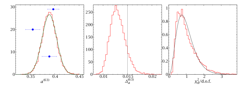
Figure b.1: Left: Probability density function of $a^{(63)}$, the estimate of exponent $a$ as obtained from a set of 63 samples. The dots with horizontal error bars are, from top to bottom: our best estimate with 768 samples, the value with the 63 samples of [janus:08b] and the mean and standard deviation of $a^{(63)}$. The continuous line is a Gaussian distribution with the same mean and variance. Centre: As in left panel, for the jackknife errors $\varDelta_{a}^{(63)}$. The vertical line marks the standard deviation of $a^{(63)}$. Right: Histogram of the $\chi^{2}_{\text{d}}$/d.o.f. for the $\xi$ fit, which had $80$ degrees of freedom. We see that there is a very large variance, indicating that the effective number of degrees of freedom is much smaller. As a comparison, we have plotted with a continuous line the chi-square distribution (per d.o.f.) for only $8$ degrees of freedom.

Therefore, we may have underestimated our errors, or there may be some bias in our methods (or in our statistics). The first source of systematic error is the dynamic cutoff method. Naturally, for the simulations with $768$ samples the cutoff point $\varLambda$ is larger. This has the effect of trading statistical uncertainty (including more noisy data at the tails) for a reduction of systematic errors, and is probably at the core of the small decrease in our error estimate.

However, the effect is large enough to merit a more detailed study, which we shall carry out with a bootstrap procedure (see, e.g., [efron:94]). Our objective is to estimate the probability distribution of $a^{(63)}$, defined as the result of computing $a$ from a statistic of $63$ samples. This can be easily done, since from our second set of simulations we have $768$ samples. Therefore, we can pick random sets of $63$ samples and determine for each set the estimate of $a^{(63)}$ and of its error $\varDelta_{a}^{(63)}$. There are $\binom{768}{63}\sim 10^{93}$ possible combinations, so our distribution of $a^{(63)}$ computed from a set of $768$ samples can be considered the ‘real’ one.

We have used $10\,000$ random sets, with which we have computed normalised histograms of $a^{(63)}$ and its errors, plotted in Figure b.1. From the first histogram we can take several conclusions:

1. The distribution of $a^{(63)}$ is Gaussian, with a very good approximation. We denote its mean by $\mathrm{E}(a^{(63)})$.

2. We were unfortunate in [janus:08b], in that the $63$ samples used therein are ‘atypical’. More precisely, the samples of [janus:08b] produce an estimate of $[a^{(63)}]$ that is $2.2$ standard deviations away from its true expectation value $\mathrm{E}(a^{(63)})$ (there is only a $3\%$ probability to obtain a larger fluctuation in Gaussianly distributed results).

3. The random variable $a^{(63)}$ seems to be a slightly biased estimator of $a$, $\mathrm{E}(a^{(63)})$ showing a small deviation from our estimate of $a$ with $768$ samples. This is probably due from the cutoff effects discussed earlier, although the fact that $a$ is obtained from a non-linear operation may also produce a small bias in the fitting procedure.

From the second histogram, representing the pdf of $\varDelta^{(63)}_{a}$, we see that the jackknife method tends to underestimate the errors somewhat (compare the mean of this distribution with the vertical line, marking the true standard deviation of $a^{(63)}$).

As a final result, we can look at the histogram of the $\chi^{2}_{\text{d}}/\text{d.o.f.}$ obtained in the $10\,000$ fits during the bootstrapping procedure. Each of these had $80$ degrees of freedom, yet the standard deviation of the distribution is much larger than that of a chi-square distribution with $80$ degrees of freedom. This supports our initial claim that fits with the diagonal chi-square procedure have a small effective number of degrees of freedom.

B.3.3.2 The full-aging exponent

Let us now consider our analysis of full aging in Section 10.2. The $\alpha(t_{\mathrm{w}})$ that we plotted in Figure 10.2 showed suspicious fluctuations (this is especially noticeable for $T=0.6$). This may lead the reader to think we have underestimated our errors when computing fits to (10.19).

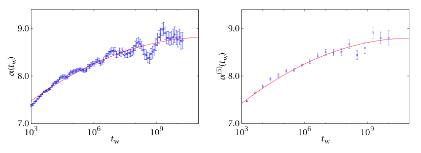
Figure b.2: Exponent $\alpha(t_{\mathrm{w}})$ for our $T=0.6$ simulations, with a fit to a quadratic polynomial in $\log t_{\mathrm{w}}$. We show on the left panel the same data as in Figure 10.2 and on the right one the result of binning the data in blocks of $5$ consecutive times.

We can check that the errors are actually correctly estimated by performing a fit of $\alpha(t_{\mathrm{w}})$ to a very smooth function. We have done this in the worst case ($T=0.6$, Figure b.2—left) with a quadratic fit

$$\alpha(t_{\mathrm{w}})=\alpha_{0}+\alpha_{1}\log t_{\mathrm{w}}+\alpha_{2}\log^{2}t_{\mathrm{w}}.$$ (b.34)

For $t_{\mathrm{w}}>10^{5}$ we have

$$\alpha_{0} =6.4(6), \alpha_{1} =0.19(8), \alpha_{2} =-0.003\,5(20),$$ (b.35)

with a diagonal chi-square of $\chi^{2}_{\text{d}}/\text{d.o.f.}=66.26/63$.

As an additional check we show in Figure b.2—right the same plot, but now binning the data in blocks of $5$ consecutive times. The resulting parameters are

$$\alpha_{0}^{(5)} =6.2(6), \alpha_{1}^{(5)} =0.20(8), \alpha_{2}^{(5)} =-0.003\,9(24),$$ (b.36)

with $\chi^{2}_{\text{d}}/\text{d.o.f.}=11.58/10$. Therefore, neither the parameters nor the value of $\chi^{2}_{\text{d}}/\text{d.o.f.}$ are affected by the binning procedure. Notice that in Figure b.2—right the wiggles in the curve seem just what they are: random fluctuations.

A second check is provided by our simulations for $T=0.7$. For this temperature, we performed two series of runs (cf. Appendix E). The first, reaching $t_{\mathrm{w}}=10^{11}$, included $63$ samples. The second, for $768$ samples, reached $t_{\mathrm{w}}=10^{10}$. We have plotted $\alpha(t_{\mathrm{w}})$ for both sets in Figure b.3. We see that, increasing the number of samples, the period of the oscillations does not change, but their amplitude decreases proportionally to the error. However, see right panel, the $\chi^{2}_{\text{d}}/\text{d.o.f.}$, which is reasonable from $t_{\mathrm{w}}\sim 10^{4}$ for $63$ samples, is not good with $768$ until $t_{\mathrm{w}}\sim 10^{8}$. This indicates that there probably is a systematic deviation from (10.19). Nevertheless, the estimates for $\alpha(t_{\mathrm{w}})$ are compatible in a much wider range.

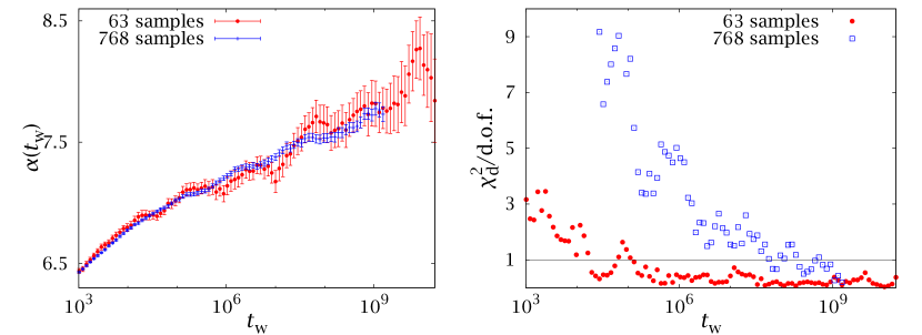
Figure b.3: Left: Estimate of $\alpha(t_{\mathrm{w}})$ in (10.19) for our $T=0.7$ simulations with $63$ and $768$ samples. Right: Values of $\chi^{2}_{\text{d}}/\text{d.o.f.}$ for both series.

B.4  Using correlations to improve the statistics: control variates

In the above section, we have discussed the difficulties posed by data correlation. However, sometimes correlations can be exploited to our advantage. A good example is the use of control variates (see [rubinstein:07] and [fernandez:09c] for a review, applied to Monte Carlo simulations).

The idea is the following, assume we want to compute some parameter $A$ and that we have a random variable $\mathcal{A}$ such that $\mathrm{E}(\mathcal{A})=A$ (that is, $\mathcal{A}$ is an unbiased estimator for $A$). Here $\mathrm{E}$ denotes the mathematical expectation, which in a Monte Carlo context can be either a thermal or a disorder average. In addition, we have an estimator $\mathcal{B}$ (the control variate) whose expectation value $B=\mathrm{E}(\mathcal{B})$ is known in advance. Then $\mathcal{A}^{\prime}=\mathcal{A}+\alpha(\mathcal{B}-B)$ is another unbiased estimator for $A$, $\mathrm{E}(\mathcal{A}^{\prime})=\mathrm{E}(\mathcal{A})=A$. Furthermore,

$$\mathrm{Var}(\mathcal{A}^{\prime})=\mathrm{Var}(\mathcal{A})+\alpha^{2}\mathrm{Var}(\mathcal{B})+2\alpha\mathrm{Cov}(\mathcal{A},\mathcal{B}),$$ (b.37)

where $\mathrm{Var}$ denotes the variance and $\mathrm{Cov}(\mathcal{A},\mathcal{B})$ the covariance of $\mathcal{A}$ and $\mathcal{B}$. It is easy to show that choosing

$$\alpha=-\frac{\mathrm{Cov}(\mathcal{A},\mathcal{B})}{\mathrm{Var}(\mathcal{B})}$$ (b.38)

minimises the variance of $\mathcal{A}^{\prime}$, so that

$$\mathrm{Var}(\mathcal{A}^{\prime}) =(1-\mathcal{R}_{\mathcal{A},\mathcal{B}}^{2})\mathrm{Var}(\mathcal{A}), \mathcal{R}_{\mathcal{A},\mathcal{B}}=\frac{\mathrm{Cov}({\mathcal{A},\mathcal{B}})}{\sqrt{\mathrm{Var}({\mathcal{A}})\mathrm{Var}({\mathcal{B}})}},$$ (b.39)

where $\mathcal{R}_{\mathcal{A},\mathcal{B}}$ is the correlation coefficient of $\mathcal{A}$ and $\mathcal{B}$. Notice that this process not only reduces statistical errors in the sought parameter, but also corrects finite-statistics biases.

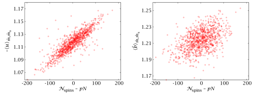
Figure b.4: Scatter plots of the energy and tethered field of individual samples against the number of spins (top panels and bottom left panel). The bottom right panel plots the staggered component of the tethered magnetic field against the $\mathcal{F}({\boldsymbol{k}})$ of Eq. (b.41) for ${\boldsymbol{k}}=(\uppi,\uppi,\uppi)$. All panels show our $1000$ samples for $L=24$ at $\beta=0.625$, $\hat{m}=0.12$ and $\hat{m}_{\text{s}}=0.5$.

We have applied this method in order to minimise the variance in the disorder average of physical quantities in our DAFF simulations of Chapter 8. For potential control variates we can consider the distribution of the vacancies $\epsilon_{\boldsymbol{x}}$ in the lattice. Indeed, we know that, for instance, the average value of spins in the lattice is

$$\overline{{\mathcal{N}}_{\text{spins}}}=pN.$$ (b.40)

More generally, the distribution of empty nodes on the lattice should be completely random, with no periodicity or correlation. We can, therefore, consider the Fourier transform of the $\epsilon_{\boldsymbol{x}}$,

$$\mathcal{F}({\boldsymbol{k}})=\sum_{\boldsymbol{x}}\epsilon_{\boldsymbol{x}}\mathrm{e}^{-\mathrm{i}{\boldsymbol{x}}\cdot{\boldsymbol{k}}}.$$ (b.41)

We have, then,

$$\overline{\mathcal{F}}(0) =\overline{{\mathcal{N}}_{\text{spins}}}=pN, \overline{\mathcal{F}}({\boldsymbol{k}}) =0,\quad{\boldsymbol{k}}\neq 0.$$ (b.42)

Once we have found viable candidates for control variates, we have to check whether they are correlated with any physical quantity. Let us start with $N_{\text{spins}}$, for which we show scatter plots in the first three panels of Figure b.4. This quantity has a strong correlation with the energy of the sample (top left) and a slight correlation with the regular component of the tethered field (top right), but no correlation at all with $\hat{b}_{\text{s}}$ (bottom left). However, see bottom right panel, this latter quantity does show a correlation with $\mathcal{F}=\mathcal{F}\bigl{(}{\boldsymbol{k}}=(\uppi,\uppi,\uppi)\bigr{)}$.

Therefore, we have used ${\mathcal{N}}_{\text{spins}}$ as a control variate for the energy and $\hat{b}$ and $\mathcal{F}$ as a control variate for $\hat{b}_{\text{s}}$. The correlation coefficients for an $L=24$ system at $\beta=0.625$, $\hat{m}=0.12$ and $\hat{m}_{\text{s}}=0.5$ are

$$\mathcal{R}_{u,{\mathcal{N}}_{\text{spins}}} =-0.85, \mathcal{R}_{\hat{b},N_{\text{spins}}} =0.47, \mathcal{R}_{\hat{b}_{\text{s}},\mathcal{F}} =-0.62.$$ (b.43)

For the energy, the resulting reduction, Eq. (b.39), is of about $50\%$. Even for $\hat{b}_{\text{s}}$ the error reduction is of about $20\%$. Recalling that the statistical error otherwise goes as $\sim 1/\sqrt{{\mathcal{N}}_{\text{samples}}}$, we see that using control variates for $\hat{b}_{\text{s}}$ is equivalent to an increase of $\approx 65\%$ in the number of samples (and, hence, in the simulation time).

Appendix C Fine tuning Tethered Monte Carlo

This chapter contains some technical details on our tethered simulations, as well as some practical recipes for the correct usage of TMC. We use the example of the $D=2$ Ising model, as in Chapter 5, except for Section C.4, which explains our numerical implementation for the DAFF.

C.1  Numerical implementation of the Metropolis scheme for the $D=2$ Ising model

We have used the Metropolis algorithm explained in Section 3.2.1. A naive implementation is completely straightforward and no different than that of canonical Metropolis (see [amit:05], for instance, for a complete working example). We can, however, significantly enhance the performance in a simple way. Indeed, using the explicit form (4.17) of the tethered weight, the spin reversal probability is

$$P(s_{\boldsymbol{x}}\to-s_{\boldsymbol{x}})=\begin{cases}0,&M^{\prime}>\hat{M},\\ \min\{1,\mathrm{e}^{\Delta S}\},&M^{\prime}\leq M,\end{cases}$$ (c.1)

where

$$\Delta S=-\beta(U^{\prime}-U)+(M^{\prime}-M)-\left(\frac{N}{2}-1\right)\log\left(1-\frac{M^{\prime}-M}{\hat{M}-M}\right)\ .$$ (c.2)

Now, in a Metropolis simulation, most of the CPU time is going to be dedicated to evaluating $\exp[\Delta S]$, which includes computing a logarithm, and therefore needs a large number of elementary operations. However, there are only a finite number of possible values for $\Delta S$.

• $(U^{\prime}-U)=-Hs_{\boldsymbol{x}}$, where $H$ is the local field around ${\boldsymbol{x}}$ and can only take $5$ different values for this model, $H=-4,-2,0,2,4$.

• $M^{\prime}=M-2s_{\boldsymbol{x}}$ and $M$ can only take $(N+1)$ values.

• The spin $s_{\boldsymbol{x}}$ itself can take only two values.

In all, we have $10(N+1)$ possible values of the Metropolis update probability (many of which are going to be zero or one, because of the constraints). This is a manageable number, so we can compute them all and store them in memory in a look-up table before starting the simulation. This way, we remove the need for computing logarithms on the fly and greatly accelerate the code.

A second note concerns the choice of the pseudorandom number generator. We originally used a $64$-bit congruential generator reported in [ossola:04]. We ran through the lattice sequentially, extracting one random number per site (although, in principle, we would only need one when $\Delta S<0$ and $\hat{M}\geq M^{\prime}$). This reproduces the conditions studied in [ossola:04, ossola:04b], where significant deviations from the expected values where found using the same generator in a $D=3$ Ising model for $N\geq 128^{3}$. Perhaps unsurprisingly, we also obtained wrong results for our larger lattices $(N=1024^{2})$. We solved the problem by repeating all our simulations with a more sophisticated generator, computed as the sum (modulo $2^{64}$) of the congruential generator and a $64$-bit version of the shift-register method reported in [parisi:85].

C.2  Sampling the $\hat{m}$ space

The first practical decision in a TMC computation is the sampling of the coordinate space, that is, how many values of $\hat{m}$ to simulate and where to put them. This is an important matter because the reconstruction of the canonical partition function (and of the canonical expectation values) involves an integral over $\exp[-N\varOmega_{N}]$, where $\varOmega_{N}$ is itself an integral of the discretised $\braket{\hat{b}}_{\hat{m}}$. A good sampling should make the discretisation errors negligible, as well as minimise the statistical ones.

Recalling the definition (4.9) of $\hat{M}$, we see that this parameter can, in principle take values in the interval $[-1,\infty)$. In practice, though, $\hat{m}\simeq m+1/2$, so the pdf $p(\hat{m})$ is going to be completely negligible outside a finite range (roughly $[-1/2,3/2]$, except for very small lattices, where we need a broader scope). In addition, see Figure 5.1, $p(\hat{m})$ is a two-peaked distribution, so values of $\hat{m}$ close to the probability maxima contribute more towards the canonical average. The peaks get narrower and closer together as $L$ grows (notice that $\varOmega_{N}$ has to be a convex function in the thermodynamical limit). It may seem that the choice of $\hat{m}$ is quite delicate (especially considering we do not know the pdf until we have run the simulation). Finally, given a fixed computational budget, is it better to compute $\braket{\hat{b}}_{\hat{m}}$ at more points or more precisely at each point with a coarser grid?

Let us assume we have measured $\braket{\hat{b}}_{\hat{m}}$ at $K$ points in a grid. Our numerical estimator $[\hat{b}]_{\hat{m}}$ at point $k$ is

$$[\hat{b}]_{k}=\braket{\hat{b}}_{k}+\eta_{k},\qquad k=1,\ldots,K.$$ (c.3)

Here $\eta_{k}$ are the statistical errors, expected to follow a Gaussian distribution and to be of similar size and statistically uncorrelated. Therefore, our numerical estimate for $\varOmega_{N}$ will be given by some quadrature formula

$$\varOmega_{N}\simeq[\varOmega_{N}]=\sum_{k=1}^{N}g_{k}\braket{\hat{b}}_{k}+\sum_{k=1}^{K}g_{k}\eta_{k}.$$ (c.4)

The first term in this equation is subject to systematical error while the second one represents the statistical fluctuations. Naively, the quadrature coefficients $g_{k}$ scale as $1/N$, so the error will scale as $1/\sqrt{N}$. This suggests that doubling the number of points is equivalent to doubling the simulation time in each one. The analysis of canonical expectation values is, however, more involved, since the errors in $\varOmega_{N}$ are going to be highly correlated for different $\hat{m}$. Therefore, we perform a numerical experiment.

We report in Table c.1 the values for the energy density $\braket{u}$ at the critical temperature for an $L=128$ lattice, obtained in two different series of runs. In the first column, we take $10^{6}$ Monte Carlo sweeps (MCS) on each point, while in the second we perform $10^{7}$ such updates. In both cases the points are evenly spaced. In the third and fourth columns we report analogous simulations, but now with a greater density of points inside the peaks. We can reach several conclusions from this table:

${\mathcal{N}}_{\text{points}}$	Uniform sampling		Improved sampling
	$10^{6}$ MCS	$10^{7}$ MCS	$10^{6}$ MCS	$10^{7}$ MCS
12	1.437 28(33)	1.437 38(11)
23	1.419 25(22)	1.419 117(6)
46	1.419 21(13)	1.419 117(43)	1.419 08(11)	1.419 107(38)
91	1.419 14(10)	1.419 093(36)	1.419 13(8)	1.419 128(31)
181	1.419 14(7)	1.419 095(28)	1.419 03(5)
451	1.419 06(5)		1.419 073(39)
901	1.419 065(33)		1.419 077(26)
1801	1.419 062(24)
Exact	1.419 076 272 086…

Table c.1: Final value for $-\langle\hat{u}\rangle$ as we change the number of points for the reconstruction of $\varOmega_{N}$ and their precision. MCS = Monte Carlo Sweeps for each point. The runs labelled ‘uniform sampling’ consist of ${\mathcal{N}}_{\text{points}}$ values of $\hat{m}$ evenly distributed in the range $[-0.4,1.4]$. The runs labelled ‘improved sampling’ have $2/3{\mathcal{N}}_{\text{points}}$ points evenly distributed in the same range, plus and additional ${\mathcal{N}}_{\text{points}}/3$ inside the peaks, effectively doubling the density in the dominant regions. The last results of each column have a similar precision, but those computed with uniform sampling required twice the simulation time. The exact value has been computed from the results of [ferdinand:69].

• If we use to low a number of points we will see a significant systematic error, no matter how precise they are.

• Once the systematic error is under control, increasing the number of evenly distributed points has an effect of $1/\sqrt{{\mathcal{N}}_{\mathrm{points}}}$ in the statistical error. This is best seen in the leftmost column. The effect is roughly the same if we increase the number of MCS in each point by the same factor (the errors of the first column are $\sim\sqrt{10}$ times greater than the corresponding ones of the second).

• If we add more points inside the peaks, the error may decrease faster than $1/\sqrt{{\mathcal{N}}_{\mathrm{points}}}$. The errors with ${\mathcal{N}}_{\text{points}}$ and uniform sampling are only slightly smaller than those with ${\mathcal{N}}_{\text{points}}/2$ and improved sampling.

We can summarise this analysis with the following prescription for the choice of $\hat{m}$:

1. Run a first simulation with enough uniformly sampled $\hat{m}$ so that the systematic error is small or unnoticeable (i.e., so that the peaks of the distribution can be roughly reconstructed and the tails are reliably sampled). We have used $\sim 50$. This may seem a big number, but we must take into account that we have only looked at the energy in Table c.1. Other quantities, such as high moments of the magnetisation or observables at a nonzero magnetic field, require that the tails of the distribution be reasonably well sampled.

2. Add a similar number of points inside the peaks of the pdf to eliminate the systematic error and reduce the statistical error.

We have found that the second step is not always necessary. In fact, for lattices up to $L=256$ we have limited ourselves to computing $51$ evenly distributed $\hat{m}$. For bigger lattices the peaks are steeper and we have added another $26$ points inside them.

This general prescription can be generalised to more complicated situations (such as the DAFF studied in Chapter 8). The rule of thumb is that the final results should not change, within the statistical errors, even if we remove several points.

A final comment concerns computation time. Obviously, it takes as much total CPU time to run $10$ simulations of length $T$ as one simulation of length $10T$. The wall-clock, defined as the physical time we have to wait for the results, is, however, $10$ times smaller in the former case, since the different tethered simulations are trivially parallelisable. Therefore, in a large-scale computation and so long as thermalisation has been ensured, it is generally better to add more points rather than extend the original ones.

C.3  Integrating over $\hat{m}$ space

The numerical implementation of (4.23) can be done in several different ways of similar numerical accuracy. Here we briefly explain our choices. Once we have the $\braket{O}_{\hat{m}_{k}}$ we need to take three steps

1. Interpolate the tethered averages as a smooth function of $\hat{m}$.

2. Integrate $\braket{\hat{b}}_{\hat{m}}$ to get $\varOmega_{N}$.

3. Use (4.4) to compute the canonical averages.

For the first step we have used a cubic spline interpolation (see, e.g., [press:92] for an implementation). We have not used the so called natural spline, which imposes vanishing curvature for $\braket{\hat{b}}_{\hat{m}}$ at $\hat{m}_{\text{max}}$ and $\hat{m}_{\text{min}}$. Instead, we have estimated the derivative of this function at both ending points with a parabolic interpolation.

In order to compute the potential $\varOmega_{N}$ we have to integrate $\braket{\hat{b}}_{\hat{m}}$ for our whole $\hat{m}$ range. In principle we could compute $\varOmega_{N}$ from

$$I_{N}(\hat{m})=\int_{\hat{m}_{\text{min}}}^{\hat{m}}\mathrm{d}\hat{m}^{\prime}\ \braket{\hat{b}}_{\hat{m}^{\prime}},$$ (c.5)

$I_{N}$ defines $\varOmega_{N}$ up to an additive normalisation constant. This expression has the disadvantage of not treating symmetrically the $\hat{m}$ range. In particular, values of $\hat{m}$ close to $\hat{m}_{\text{min}}$ will have smaller errors than those close to $\hat{m}_{\text{max}}$. In order to avoid this problem, we use the average of the integral in both directions,

$$I_{N}(\hat{m})=\frac{1}{2}\left(\int_{\hat{m}_{\text{min}}}^{\hat{m}}\mathrm{d}\hat{m}^{\prime}\ \braket{\hat{b}}_{\hat{m}^{\prime}}-\int_{\hat{m}}^{\hat{m}_{\text{max}}}\mathrm{d}\hat{m}^{\prime}\ \braket{\hat{b}}_{\hat{m}^{\prime}}\right).$$ (c.6)

Notice that, assuming $\hat{m}_{\text{min}}$ and $\hat{m}_{\text{max}}$ are far enough as to have negligible probability, both (c.5) and (c.6) are equivalent, considering the potential nature of $\Omega_{N}$. It is only when we consider numerical issues that the second is preferable.

We now normalise the pdf,

$$\mathcal{C}=\int_{\hat{m}_{\text{min}}}^{\hat{m}_{\text{max}}}\mathrm{d}\hat{m}\ \exp[-NI_{N}(\hat{m})],$$ (c.7)

so that

$$\varOmega_{N}(\hat{m})=I_{N}(\hat{m})-\frac{1}{N}\log\mathcal{C}.$$ (c.8)

Some comments are in order. First of all, naively applying this interpolation scheme for the exponential, $p(\hat{m})=\exp[-N\varOmega_{N}(\hat{m})]$, could introduce strong integration errors. Fortunately, this can be easily solved by accurately representing $\varOmega_{N}$, which is a smooth function (recall the curve in logarithmic scale of Figure 3.1).

In particular, since we have represented the tethered field with a cubic spline, $\varOmega_{N}$ is a fourth order polynomial between each pair of simulated points, which can be exactly computed. To avoid losing precision, we evaluate $\varOmega_{N}(\hat{m})$ in an extended grid that includes $3$ equally spaced intermediate points between each pair of simulated values of $\hat{m}$. This way the Lagrange interpolating polynomial for each segment of the extended lattice (two original points plus three intermediate ones) represents the exact integral of our spline.

Of course, the pdf, $\exp[-N\varOmega_{N}(\hat{m})]$, is not a polynomial anymore. It is, however, a smooth function, so a self consistent Romberg method [press:92] provides an estimate of the integral (4.4) with any required numerical accuracy. Notice that this yields the basically exact results for a given interpolation of $\braket{\hat{b}}_{\hat{m}}$, but it does not cure any discretisation errors introduced by the spline, which should be minimised with the prescription of the previous section.

Throughout this process, we estimate errors with the jackknife method (see Appendix B). For instance, we compute and integrate a different cubic spline for each jackknife block. This way, data correlation is safely taken into account when estimating the statistical errors.

Typically, even with a very moderate effort, the Romberg integration error has been much smaller than the statistical one. There is one exception: the fluctuation-dissipation formulas, such as (5.2), because of the large cancellations between the two terms. To solve this problem, we have computed the fluctuation-dissipation formula as a sum of two squares:

$$N^{-1}C=\braket{\hat{u}^{2}}-\braket{\hat{u}}^{2} =\int\mathrm{d}\hat{m}\ p(\hat{m})\left[\braket{\hat{u}^{2}}_{\hat{m}}-\braket{\hat{u}}^{2}_{\hat{m}}+\braket{\hat{u}}^{2}_{\hat{m}}-\braket{\hat{u}}^{2}\right]$$

$$=\int\mathrm{d}\hat{m}\ p(\hat{m})\left[\braket{(\hat{u}-\braket{\hat{u}}_{\hat{m}})^{2}}_{\hat{m}}+\left(\braket{\hat{u}}_{\hat{m}}-\braket{\hat{u}}\right)^{2}\right].$$ (c.9)

In spite of this, as a consistency check, we have also employed the original equation and forced the Romberg integral to yield the same value, by reducing its tolerance.

It is sometimes interesting to compute high moments of the magnetisation. One obvious possibility is to measure the instantaneous values for $m^{\ell}(\hat{m};\{\sigma_{\boldsymbol{x}}\})$ during the simulation and then compute the tethered and canonical averages as usual. But TMC provides an alternative way of calculating $\langle m^{\ell}\rangle$. Indeed, we have the whole pdf $p(\hat{m})$ and we know that $\hat{M}=M+R$. Now, the moments for $R$ can be easily obtained analytically, so it suffices to compute $\langle\hat{m}^{\ell}\rangle$ to reconstruct $\langle m^{\ell}\rangle$ without any need for individual measurements of $m^{\ell}$. For example,

$$\langle m^{2}\rangle =\langle(\hat{m}-1/2)^{2}\rangle-\frac{1}{2N}\ .$$ (c.10)

$$\langle m^{4}\rangle =\langle(\hat{m}-1/2)^{4}\rangle-\frac{3}{N}\langle m^{2}\rangle-\frac{3}{4N^{2}}+\frac{3}{N^{3}}\ .$$ (c.11)

These formulas are valid for the symmetric phase, where $\langle m\rangle=0$. We have computed the moments of the magnetisation up to $\langle m^{8}\rangle$, both from individual measurements and with this procedure, and the results are identical. This will not be at all surprising once we see Section 5.5, where it is shown that the correlation time for $\langle m\rangle_{\hat{m}}$ is $<1$ (which means that the uncertainty in $p(\hat{m})$ is going to determine the total error).

C.4  Numerical implementation of TMC for the DAFF

The tethered simulations of the DAFF were also carried out with a Metropolis algorithm. In principle we could have used the, potentially more efficient, cluster method studied in detail in Appendix 6. Indeed, the formulation for the DAFF follows the same steps as that for the Ising model , with the exceptions that the clusters are now of constant staggered spin and that we now have two tethered quantities, so now the cluster flipping weight is

$$\omega(\{S_{i}\})\propto\gamma(\hat{m},m)\gamma(\hat{m}_{\text{s}},m_{\text{s}}),$$ (c.12)

where $\gamma(\hat{x},x)$ was defined in (4.33). Unfortunately, for the relevant temperature and magnetisation regimes for the DAFF, the spin configurations are not well suited to cluster methods. In particular (see Section 8.6), the whole configuration is dominated by two very large clusters of opposite staggered spin, of similar size for $\hat{m}_{\text{s}}=0.5$ and with one dominant cluster in magnetised regions. What few spins remain outside them are scattered in a few very small clusters and a large number of single-spin ones. In these conditions, and given the stringent constraints on $(m,m_{\text{s}})$ imposed by (c.12), the cluster flipping would only invert loose spins and leave the large clusters untouched.

We must, therefore, stick with the Metropolis scheme. Still, there are a few things we can do to optimise the simulation. First of all, we avoid computing logarithms when evaluating the Metropolis acceptance probability with the preparation of look-up tables, as discussed in Section C.1. Now we have to consider $\mathcal{O}(N^{2})$ values for $(M,M_{\text{s}})$, so we cannot fit all the possibilities in a single array. However, since the contributions of $U$, $M$ and $M_{\text{s}}$ to the update probability are factorised, we can simply prepare one look-up table for each of these quantities and evaluate the whole Metropolis probability with a simple multiplication.

The peculiarities of the DAFF in the tethered formalism afford us an additional possible optimisation. It turns out that the Metropolis acceptance is very low, of about $10\%$ in most cases (this is mainly due to the regular magnetisation, which is in a very constrained regime due to the high applied fields that we consider). In addition, with the look-up table method, the computation of the acceptance probability is faster than the generation of a single pseudorandom number.

With this in mind, let us suppose we are performing a sweep of the whole lattice, updating nodes $0$ to $N-1$. Let us call $p_{i}$ the probability of flipping spin $i$ and $q_{i}=1-p_{i}$ the probability of rejecting the change. Then, the probability of leaving the spins from $i=k$ to $i=s$ unchanged

$$Q_{k,s}=\prod_{j=k}^{s}q_{j}=Q_{k,s-1}q_{s}.$$ (c.13)

Therefore, we can define a ‘survival’ Metropolis scheme in the following way:

• For $k=0,\ldots,N-1$ do

  1. Generate a single pseudorandom number $\mathcal{R}\in[0,1)$.

  2. Compute $Q_{k,s}$ until $Q_{k,s-1}>\mathcal{R}\geq Q_{k,s}$. Then flip spin $s$.

  3. Set $k=s+1$.

This algorithm obviously satisfies the balance condition for a Monte Carlo method and should be more efficient than the standard Metropolis for low acceptance probabilities. In practice, modern compilers make this a strongly device-dependent optimisation. We have found that for modern Intel processors, using the Intel C compiler icc, the gain is negligible for the acceptance of $10\%$ found in our DAFF simulations. However, more than half of our simulations (over $3.5$ million CPU hours) were carried out on the Mare Nostrum supercomputer, of different design, where the survival version of the Metropolis scheme nets us a $30$ to $40$% acceleration.

Finally, we take one parallel tempering (Section A.3.1) step for each lattice update, attempting to exchange configurations for the same $(\hat{m},\hat{m}_{\text{s}})$ but different $\beta$. In the tethered weight (4.17), the factors that depend on the magnetisation are independent of $\beta$, so the parallel tempering acceptance probability is exactly the same as that for a canonical simulation, given by (a.30). For our longest simulations, we use a parallel version of our code that runs the Metropolis update of each of the participating configurations in a different processor. When the whole lattice has been updated, the energies and temperatures of each configuration are sent to the master process (with MPI, Message Passing Interface), which performs the parallel tempering update and sends back the new temperatures. In this way the total CPU time is of course unchanged, but the wall-clock is reduced by a factor ${\mathcal{N}}_{T}$.

Appendix D The Janus computer

The Monte Carlo simulation of complex disordered systems has an unquenchable thirst for computing power. Any acceleration due to innovations in computer design is immediately exhausted. In addition, the terrible scaling properties of the characteristic times (often exponential, as we pointed out in Chapter 3) mean that, in order to obtain a qualitative improvement in the data, one needs an acceleration of orders of magnitude.

In these conditions, the investigation on new, optimised, Monte Carlo methods in not only necessary but also rewarding, as we saw with our examination of the Tethered Monte Carlo method during Part II of this dissertation. Sometimes, however, devising ingenious dynamical algorithms is not an option.

A prime example of this issue is the non-equilibrium dynamics of spin glasses. Here, we face the following constraints

• The interesting physical phenomena occur at macroscopic times, with the typical experimental scale ranging from a few seconds to a few hours.

• The physical dynamics can be faithfully simulated with heat bath or Metropolis dynamics, but each MCS is equivalent to only $\sim 10^{-12}$ s [mydosh:93].

• One has to simulate very large lattices, to keep the system in a truly off-equilibrium regime, free of finite-size effects. Therefore, each MCS takes some time.

Notice that it is not easy to see how one could improve this situation with a clever update algorithm, since we want to reproduce the physical dynamics.

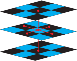
Figure d.1: Division of the spin-glass lattice in a checkerboard scheme. The first neighbours are always the opposite colour of the site, so sites of the same colour can be updated at the same time.

Thankfully, the physics of the spin glass provide a different avenue for acceleration: parallelisation. Indeed, the nearest-neighbours nature of the interaction means that we can divide each plane of the lattice in a checkerboard scheme (Figure d.1), with sites of the same colour being statistically independent from one another. That is, one could in principle update the whole lattice in two steps: first all the black sites at once and then all the white sites at once.

The problem with this idealised scheme is that conventional computers (CPUs) are simply not equipped to handle it:

• CPUs are optimised for operations on long data words, but we need (i) operations on single bits (the spins) (ii) variables that only appear in a small number of states (the local field needed to compute the update probability).

• The memory architecture does not permit the processor to gather all the necessary information quickly enough.

• We need one random number for each node that we update, so random-number generation is another bottleneck.

Sharing the computation across several CPUs (making each handle one portion of the lattice) does not work due to communication limitations: even if we only need small chunks of data, they have to be accessed extremely often.

One possible answer to this problem is designing a special-purpose computer, whose architecture is optimised for simulations of spin systems. We note that this idea is not new, custom computers have been used in statistical mechanics for some time [ogielski:85, cruz:01]. The Janus computer, fruit of a collaboration between physicists and engineers in the universities of Zaragoza, Complutense de Madrid and Extremadura (in Spain) and Ferrara and Rome 1 ‘La Sapienza’ (in Italy), is one such custom machine.

Since the author was not involved in the hardware design or the low-level programming of the machine, just in the physical analysis of the simulations, this is not the place to give a detailed account of the machine. We shall only consider some brief notions to understand why Janus can outperform conventional computers. The interested reader is referred to [janus:06, janus:09] for details on the architecture and to [janus:08] for an explanation of the implementation of the Monte Carlo simulation. See also the doctoral dissertation of F. Mantovani [mantovani:08].

The solution adopted by Janus consists in replacing the conventional CPUs by Field Programmable Gate Arrays (FPGAs) as computing nodes. These devices offer a large number of reconfigurable logic resources, so they can be divided into many update engines, each taking care of the update of one spin.

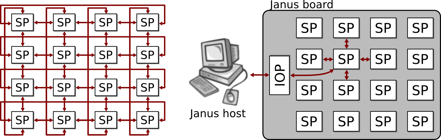
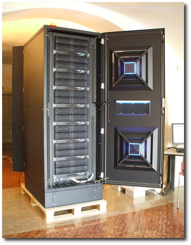
Figure d.2: Board of the Janus computer. Each of the $16$ scientific processors (SPs) is an FPGA. These are connected along nearest-neighbour links, with periodic boundary conditions. The board includes an input/output processor.

Figure d.3: The complete Janus computer.

The FPGAs are grouped in $4\times 4$ arrays, forming boards (Figure d.3). Each board includes data links among nearest neighbours and an input/output processor (IOP), whose job is to distribute work among the computing nodes and gather the results. There is a standard PC (called host) for each two boards, which acts as the interface and storage element. The whole Janus computer consists of $16$ boards (a total of $256$ processors) in one rack (Figure d.3).

In the basic implementation for non-equilibrium dynamics, each FPGA simulates two replicas of one sample, divided in the checkerboard scheme. The implementation seeks to maximise the number of spins that can be updated in each clock cycle. In particular, each FPGA can be divided in $1024$ update engines. Each of them takes the following steps

1. Reads as input $6$ nearest neighbours and the corresponding $6$ couplings.

2. Computes the local field and addresses a pre-computed look-up table (cf. Section C.1).

3. Compares the result with a freshly generated random number.

4. Sets the new value for the spin.

This whole process is pipelineable so that each of the $1024$ update engine updates one spin per clock cycle (notice that this requires a clever memory architecture, so the needed information can be accessed with no latency).

Another potential bottleneck is the generation of random numbers. As we indicated above, we need one random number for each spin of the $1024$ spins that we update in each clock cycle. For these, we use the Parisi-Rapuano shift-register generator [parisi:85]. We have a wheel $I(k)$ of $62$ numbers ($32$-bit integers). Then, in order to generate a random number $R(K)$ we perform the following operation

$$R(k) =\bigl{(}I(k-24)+I(k-55)\bigr{)}\otimes I(k-61).$$ (d.1)

Then, the wheel is shifted (we increase $k$) and update the $k$ position with the previously computed sum

$$I(k)=I(k-24)+I(k-55).$$ (d.2)

The value of $k$ is, of course, always taken modulo $62$.

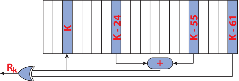
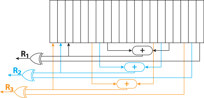
Figure d.4: Left: One step of the Parisi-Rapuano generator, implemented through a logical circuit. Right: Nested generation of three random numbers at once with the same Parisi-Rapuano wheel. At the cost of complicating this circuit, Janus generates up to $96$ random numbers per wheel per clock cycle.

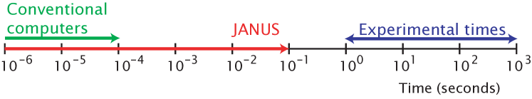
Figure d.5: Comparison of the time scales accessible to Janus and to conventional computers.

The interesting feature of this generator is that it can be easily implemented through a logic circuit (Figure d.4—left). More than that, at the cost of complicating the circuit, we can consider the simultaneous generation of many random numbers from the same wheel —several iterations of (d.1) and (d.2)— by setting up a cascade-structured combinatorial logic. This is represented for the simultaneous generation of three random numbers in Figure d.4—right. In the actual implementation, Janus is capable of generating $96$ random numbers for each wheel in each clock cycle (we still need to keep several wheels turning at the same time to keep up with the needs of the update engines).

D.1  Performance

Janus is capable of simulating a system of size up to $L=96$ in each FPGA. The above-outlined implementation is capable of exhausting $88\%$ of the available logic resources. The clock frequency of the machine is of $62.5$ MHz, so the performance of each FPGA is

$$\frac{16\text{ ns}}{1\text{ cycle}}\times\frac{1\text{ cycle}}{1024\text{ spins}}\approx 16\text{ ps/spin}$$ (d.3)

This number is, however, too abstract. One can update many spins per second by simply running many independent simulations at once, without accelerating any of them. The real measure of the performance of a computer (or an implementation) is the new physics to which it grants us access. In this sense, in the above implementation Janus is capable of simulating $256$ samples of an $L=80$ Edwards-Anderson spin glass for $10^{11}$ MCS in less than a month, a time long enough to understand what happens at the experimental scale, as we see in Chapter 10 (see Figure d.5). We also note that one can simulate even larger systems by sharing the workload among several FPGAs. For instance, a Janus board can simulate an $L=256$ lattice for $10^{10}$ MCS in less than ten days. Notice that this means that fewer samples can be simulated at once, but this is of no consequence due to the self-averaging nature of the physical observables.

Let us stress that Janus is optimised for accelerating the simulation of a single sample. If all one needs is to run many samples for a comparatively short time each —as is commonly the case for critical-point studies— Janus is also going to be very efficient, but there are simpler alternatives (the most popular being asynchronous multi-spin coding in CPUs or even graphic cards). In this dissertation, we consider also equilibrium simulation with Janus, but these are in the low-temperature regime where the thermalisation time for each sample is exceedingly long (cf. Appendix E).

We finally note that, aside from the simulations for the Edwards-Anderson spin glass with Ising spins reported in Appendix E, Janus has been used to simulate the Potts spin glass (where the spins can take several values, not just $\pm 1$) [janus:09c, janus:10c]. In this case, the gain factor with respect to conventional PCs is even greater.

Appendix E Our spin-glass simulations: parameters and thermalisation

We report in this Appendix the parameters of our spin-glass simulations and give some technical details on our logistics and (in the case of the ones in equilibrium) thermalisation tests.

E.1  Non-equilibrium simulations

$L$	$T$	$\mathcal{N}_{\text{HB}}$	$\mathcal{N}_{\text{samples}}$
$80$	$0.6$	$10^{11}$	$96$
$80$	$0.7$	$10^{11}$	$63$
80	0.7	$10^{10}$	768
80	0.8	${10}^{11}$	96
$80$	$1.1$	$4.2\times 10^{9}$	$32$
$40$	$0.8$	$2.2\times 10^{8}$	$2218$

Table e.1: Parameters the non-equilibrium simulations studied in this dissertation. The overall wall-clock time needed was less than six weeks.

We have simulated the direct quench protocol explained in Chapter 9 for several temperatures. We have used heat bath dynamics, in the highly parallelised implementation described in Appendix D. The parameters of these runs are included in Table e.1.

We have used lattices of linear size $L=80$, simulating two real replicas for each sample. In a first simulation campaign, originally reported in [janus:08b], we ran one sample in each of our $256$ FPGAs for just under one month, resulting in $96$ samples for $T=0.6,0.8$, $63$ samples for $T=0.7$ and $32$ for $T=1.1\approx T_{\text{c}}$. Our wall-clock time of $24$ days was enough to reach $10^{11}$ MCS for our subcritical simulations. At the critical point we only ran for $4.2\times 10^{9}$ MCS, using the freed-up time to run some shorter simulations for smaller lattices. These were used exclusively to check for finite-size effects (cf. Section 10.3.2).

We were interested in two kinds of dynamics: those at the critical temperature and those representative of the low-temperature phase. In the latter, one is interested in a temperature low enough not to be dominated by critical effects. However, the lower the temperature, the slower the dynamics (where the speed is measured by the growth rate of the coherence length). Since one is interested in seeing as large a coherence length as possible, one should try to find a middle ground. After analysing the results of this first batch of runs in [janus:08b], we decided that $T=0.7$ provided the best compromise. Therefore, we carried out a new set of simulations at this temperature, increasing the number of simulated samples by an order of magnitude. In these new runs, first reported in [janus:09b], we took only $10^{10}$ MCS, because after that time we could begin to resolve some finite-size effects in the coherence length growth at that temperature. When giving non-equilibrium results at $T=0.7$, we shall always refer to this larger set of runs, unless we say otherwise.

We note that $T=0.7$ is also the lowest temperature at which we could safely thermalise our largest samples in our equilibrium simulations (cf. Section E.2, below). Therefore, this should be considered as our main working temperature and will, in particular, be the one we consider when establishing the quantitative statics-dynamics equivalence, one of our main results.

Finally, let us give some logistical notes. Some of the physical quantities we study are time-consuming to measure and some are even functions of the configurations at different times. Therefore, rather than taking complex measurements during the simulation (online) we saved to disk the spin configurations at logarithmically spaced times. In particular, we stored all the information at times $[2^{i/4}]+[2^{j/4}]$, with integer $i$ and $j$ (the square brackets denote the integer part). This choice was made so that our $t$ and $t_{\mathrm{w}}$ (cf. Chapter 9) could be both studied in a logarithmic scale.

E.2  Equilibrium simulations

E.2.1 Set-up of the simulations

For our equilibrium simulations we used the parallel tempering algorithm described in Appendix A. In this case we simulated four real replicas for each sample (in order to have better statistics for some fine analyses, as well as for constructing unbiased estimators for some sophisticated observables).

The parallel tempering was coupled to heat bath dynamics. The implementation in this case was a little different than that explained for the non-equilibrium dynamics in Appendix D. In particular, since we had to run many temperatures for each replica, each FPGA simulated just one replica, so each sample was spread across four computing cores. Due to the special architecture of Janus, the parallel tempering step is not costless, as was the case for the DAFF. This is because the FPGAs first have to compute the total energy for each temperature. We thus equilibrate the computational cost of both updates by performing $10$ heat bath steps for each parallel tempering update. This hardly affects the efficiency of the parallel tempering scheme.

As was the case in our off-equilibrium dynamics simulations, most of the analyses were performed offline. In particular, for the shortest simulations (the samples that do not need extending after applying our thermalisation criteria) we stored on disk about $\sim 100$ evenly spaced configurations. This number grew proportionally to the length in the case of extended runs. Notice that this is in stark contrast with the DAFF, where we just saved the last configuration to act as a checkpoint for possible extensions.

In particular, we needed many configurations on disk to perform the analysis of fixed-$q$ correlation functions, as we explain in Section E.2.3.

Finally, for a few specific samples (one for $L=24$ and four for $L=32$) the wall-clock time required to fulfil our thermalisation criteria (cf. Appendix A) was exceedingly long, more than six months. For these cases we used a special low-level code that spread the different temperatures for each replica across several FPGAs, thus speeding up the simulation (recall that Janus has very fast connections between the FPGAs on the same board).

For the smaller lattices ($L\leq 12$) we ran the simulations on Terminus, the computing cluster of the BIFI. Even if these were very small systems, we thermalised them down to extremely low temperatures, so the simulation time was far from negligible.

E.2.2 Parameters of our simulations

$L$	$T_{\mathrm{min}}$	$T_{\mathrm{max}}$	${\mathcal{N}}_{T}$	${\mathcal{N}}_{\mathrm{mes}}$	${\mathcal{N}}_{\mathrm{HB}}^{\mathrm{min}}$	${\mathcal{N}}_{\mathrm{HB}}^{\mathrm{max}}$	${\mathcal{N}}_{\mathrm{HB}}^{\mathrm{med}}$	${\mathcal{N}}_{\mathrm{s}}$	System
8	0.150	1.575	10	$10^{3}$	$5.0\!\times\!10^{6}$	$8.30\!\times\!10^{8}$	$7.82\!\times\!10^{6}$	4000	PC
8	0.245	1.575	8	$10^{3}$	$1.0\!\times\!10^{6}$	$6.48\!\times\!10^{8}$	$2.30\!\times\!10^{6}$	4000	PC
12	0.414	1.575	12	$5\!\times\!10^{3}$	$1.0\!\times\!10^{7}$	$1.53\!\times\!10^{10}$	$3.13\!\times\!10^{7}$	4000	PC
16	0.479	1.575	16	$10^{5}$	$4.0\!\times\!10^{8}$	$2.79\!\times\!10^{11}$	$9.71\!\times\!10^{8}$	4000	Janus
24	0.625	1.600	28	$10^{5}$	$1.0\!\times\!10^{9}$	$1.81\!\times\!10^{12}$	$4.02\!\times\!10^{9}$	4000	Janus
32	0.703	1.549	34	$2\!\times\!10^{5}$	$4.0\!\times\!10^{9}$	$7.68\!\times\!10^{11}$	$1.90\!\times\!10^{10}$	1000	Janus
32	0.985	1.574	24	$2\!\times\!10^{5}$	$1.0\!\times\!10^{8}$	$4.40\!\times\!10^{9}$	$1.16\!\times\!10^{8}$	1000	Janus

Table e.2: Parameters of our spin-glass parallel tempering simulations. In all cases we have simulated four independent real replicas per sample. The $\mathcal{N}_{T}$ temperatures are uniformly distributed between $T_{\mathrm{min}}$ and $T_{\mathrm{max}}$ (except for the runs of the first row, which have all the temperatures of the second one plus $T=0.150$ and $T=0.340$). In this table ${\mathcal{N}}_{\mathrm{mes}}$ is the number of Monte Carlo Steps between measurements (one MCS consists of $10$ heat-bath updates and $1$ parallel-tempering update). The simulation length was adapted to the thermalisation time of each sample, using the methods of Appendix A. The table shows the minimum, maximum and medium simulation times (${\mathcal{N}}_{\mathrm{HB}}$) for each lattice, in heat-bath steps. Lattice sizes $L=8,12$ were simulated on conventional PCs, while sizes $L=16,24,32$ were simulated on Janus. Whenever we have two runs with different $T_{\mathrm{min}}$ for the same $L$ the sets of simulated samples are the same for both. The total spin updates for all lattice sizes sum $1.1\times 10^{20}$. It is interesting to compare the length of these simulations with the ones for the DAFF in Table 8.1.

In our DAFF simulations, we set-up our parallel tempering scheme with a very high maximum temperature, where the copies of the system achieved decorrelation very fast.

Here, however, we are not interested in the critical point, but rather in the low-temperature physics, which makes thermalisation all the more difficult. For that reason, the simulations are several orders of magnitude longer than in the DAFF’s case and, hence, for the same ratio of autocorrelation time at $T_{\text{max}}$ over total simulation time we do not need to reach such high temperatures. Still, we can perform a quantitative analysis in order to justify our parameters (which can be seen in Table e.2).

Following Ogielski [ogielski:85], the equilibrium autocorrelation time in the thermodynamic limit is taken from a power law to a critical divergence

$$\tau_{\text{HB}}(T)\sim(T-T_{\text{c}})^{-z\nu}\,.$$ (e.1)

For instance, for the maximum temperature used in our largest lattice, Ogielski found $\tau_{\text{HB}}\sim 10^{5}$. This is several orders of magnitude shorter than our shortest simulations in Table e.2.

We chose the minimum temperature so that the whole simulation campaign took about $200$ days of the whole Janus machine and so that the lowest temperature scaled as $T_{\text{c}}-T_{\text{min}}\sim L^{-1/\nu}$. With $4000$ samples for $L=16,24$ and $1000$ for $L=32$, this resulted in $T_{\text{min}}=0.479,0.625,0.703$, respectively.

As we cautioned in Appendix A, trying to optimise the choice of the remaining parameters (number and distribution of the intermediate temperatures) is an unrewarding task. We dedicated several weeks to testing several combinations, mainly by modifying the number $\mathcal{N}_{T}$ of temperatures so that the acceptance of the parallel tempering exchanges varied between $7\%$ and $30\%$. Perhaps against conventional wisdom, taking into account that the computational effort at fixed $\mathcal{N}_{\text{HB}}$ is proportional to $\mathcal{N}_{T}$, we found that the efficiency hardly changed. Eventually, we settled for a spacing of temperatures that produced acceptances of $\approx 20\%$. This both avoided unconventionally low acceptances and saved disk space.

E.2.3 Offline evaluation of observables

As we indicated before, most of our analyses were performed offline, on previously stored spin-glass configurations. In particular, the computation of conditional correlation functions $C_{4}(\boldsymbol{r}|q)$ —Eq. 10.58— was not only time-consuming but also required a lot of unrefined data. This was a problem, due to the scarcity of stored configurations. In fact, for the samples that were simulated only for the minimum simulation time, we had only ${\mathcal{N}}_{\mathrm{conf}}\sim 100$ configurations stored on disk (ranging from ${\mathcal{N}}_{\mathrm{conf}}=10$ for $L=12$ to ${\mathcal{N}}_{\mathrm{conf}}=200$ in the case $L=32$). We regard the second half (in a Monte Carlo time sense) of these configurations as well thermalised. Yet, when forming the overlap field, one needs only that the two spin configurations, $\{s_{\boldsymbol{x}}^{(1)}\}$ and $\{s_{\boldsymbol{x}}^{(2)}\}$, be thermalised and independent. Clearly enough, as long as the two configurations belong to different real replicas and belong to the second half of the Monte Carlo history they will be suitable. There is no need that the two configurations were obtained at the same Monte Carlo time (as it is done for the online analyses). Furthermore, the four real replicas offer us 6 pair combinations. Hence, we had at least $6\times({\mathcal{N}}_{\mathrm{conf}}/2)^{2}\sim 10000$ ($60000$ for $L=32$) measurements to estimate the overlaps and the correlation functions. We used the Fast Fourier Transform to speed up the computation of the spatial correlations. For those samples that had more configurations (because their total simulation time exceeded ${\mathcal{N}}_{\mathrm{min}}^{\mathrm{HB}}$), we considered nevertheless ${\mathcal{N}}_{\mathrm{conf}}/2$ configurations evenly spaced along the full second half of the simulation.

For some quantities, such as the spin overlaps, we did have a large number of online measurements. Therefore, When some quantity, for instance the $p(q)$, could be computed in either way, online or offline, we have compared them. The two ways turn out to be not only compatible, but also equivalent from the point of view of the statistical errors. As an example of this let us compute the following quantity:

$$\sigma_{\mathrm{link}}^{2}=\overline{\langle Q_{\mathrm{link}}^{2}\rangle}-\overline{\langle Q_{\mathrm{link}}\rangle}^{2}.$$ (e.2)

For $L=32$, $T=0.703$, the value of $\sigma_{\mathrm{link}}^{2}$ computed from online measurements of $Q_{\mathrm{link}}$ and $Q_{\mathrm{link}}^{2}$ is

$$N\sigma_{\mathrm{link,online}}^{2}=50.88(90).$$ (e.3)

We could now recompute this value from offline measurements of $Q_{\mathrm{link}}$ and $Q_{\mathrm{link}}^{2}$. Instead, we are going to use (11.32), which involves the intermediate step of computing conditional expectation values and variances at fixed $q$ and then integrating with $p(q)$. This will serve as a test both of the offline measurements’ precision and of our Gaussian convolution method for the definition of fixed-$q$ quantities. The result is

$$N\sigma_{\mathrm{link,conf}}^{2}=50.81(90),$$ (e.4)

The precision of $\sigma_{\mathrm{link,online}}^{2}$ and $\sigma_{\mathrm{link,conf}}^{2}$ is the same and the difference less than $10\%$ of the error bar, even though we only analysed $100$ configurations per sample for the second one. Of course, both determinations are very highly correlated, so the uncertainty in their difference is actually much smaller than their individual errors. Computing the difference for each jackknife block we see that

$$N[\sigma_{\mathrm{link,conf}}^{2}-\sigma_{\mathrm{link,online}}^{2}]=-0.065(79),$$ (e.5)

which is indeed compatible with zero.

A final issue is the comparison of data computed in different system sizes at the same temperatures. Unfortunately the grids of temperatures that we used for the different $L$ differ. Hence we have interpolated our data by means of a cubic spline.

E.2.4 Thermalisation

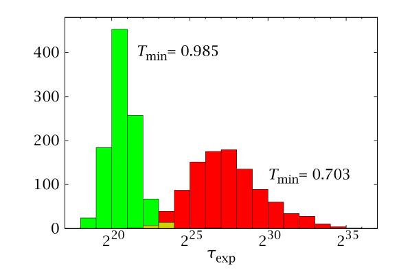
Figure e.1: Histogram of exponential autocorrelation times for our simulations of the $L=32$ lattice (1000 samples).

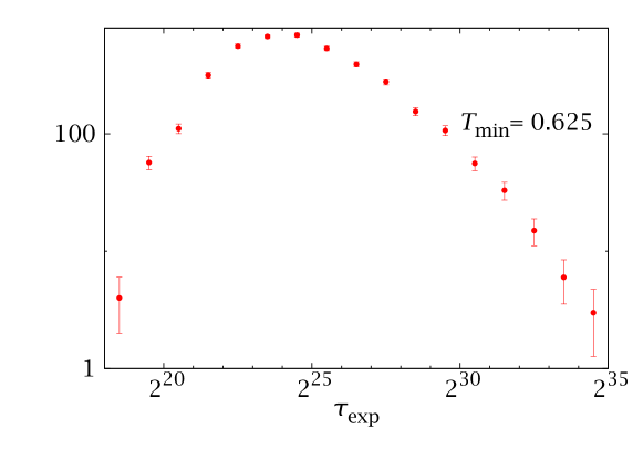
Figure e.2: Logarithm of the histogram of exponential autocorrelation times for our simulations of the $L=24$ lattice (4000 samples). Mind the behaviour of the long-times tail.

We have followed the thermalisation protocol detailed in Section A.3.3. Figure e.1 shows the histogram of exponential autocorrelation times for our $L=32$ simulations. As with the DAFF, we need to use logarithmic bins. Notice the dramatic increase of the $\tau_{\text{exp}}$ when decreasing the minimum temperature of the simulation. In Figure e.2 we plot the logarithm of the histogram to show the exponential behaviour of the long-times tail. This result gives confidence that rare events with extremely large correlation times are at least exponentially suppressed.

E.2.4.1 Thermalisation tests

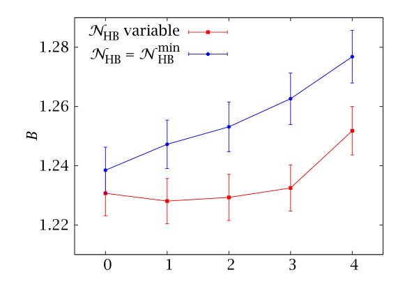
Figure e.3: Evolution of the Binder parameter for $L=32$, $T=0.703$ using $\log_{2}$ binning. The blue curve (circles) is the result of stopping at step 1 of our thermalisation protocol (i.e., all samples simulated for a fixed time of $4\!\times\!10^{9}$ heat-bath updates). The red curve (squares) is the result of completing all the steps, which implies an increase of roughly 150% in simulation time.

We consider in this section thermalisation tests directly based on physically meaningful quantities.

We start by the traditional $\log_{2}$-binning procedure of Section A.3, illustrated in Figure e.3 for the Binder ratio of Eq. (11.1), which is especially sensitive to rare events and, therefore, to possible thermalisation biases. In the figure we show two curves, both for $L=32$ and $T=T_{\text{min}}=0.703$. The blue one, with circles, is the result of stopping at step one in our thermalisation protocol of Section A.3.3 and shows a poorly thermalised ensemble. The situation improves dramatically if we follow the simulation protocol to the end, simulating each sample for a time proportional to its autocorrelation time. Notice that, thanks to our choice of ${\mathcal{N}}^{\text{min}}_{\text{HB}}$, the simulation time for most samples has not increased. If we first rescale the data according to total simulation length and average for equal rescaled time, the $\log_{2}$-binning gives four steps of stability within errors. That is to say: we obtain the Binder parameter without thermalisation bias just discarding $1/16$ of the history. Regarding $B$, then, our requirement of $12\tau_{\text{exp}}$ has been excessive.

In retrospect, shorter simulations would have produced indistinguishable physical results for most observables. We do not regret our choices, however, as we plan to use these thermalised configurations in the future [janus:xx] for very delicate analyses (such as temperature chaos), which are probably much more sensitive to thermalisation effects.

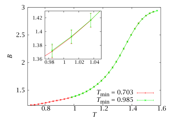
Figure e.4: Binder ratio as a function of the temperature for $L=32$. The good overlap between two different simulations (one of them in the much easier critical region) is a further thermalisation check. We use the same set of 1000 samples.

A different test can be performed by comparing the difficult low-temperature simulations of our largest lattice with simulations of the same samples in the much easier critical region. A faulty thermalisation (for instance, a configuration remains trapped at low temperatures) could be observable as inconsistencies in the values of quantities in common temperatures. In Figure e.4 we show the Binder parameter as a function of temperature for the two simulations with $L=32$ (see Table e.2). The agreement between both simulations is excellent.

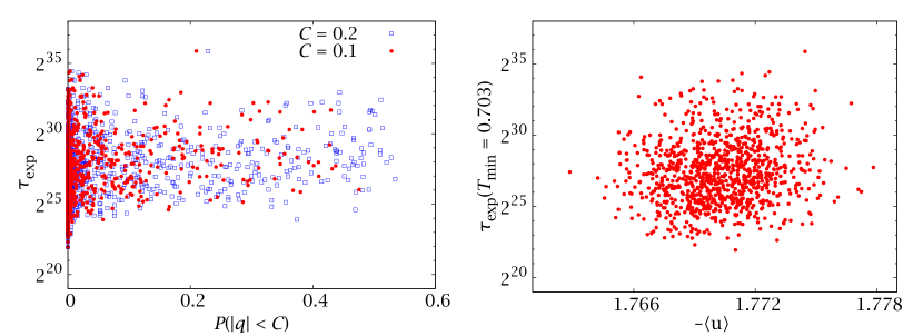
Figure e.5: Left: Scatter plot of the exponential autocorrelation time against the probability that the overlap be less than a small quantity at $T=0.703$, for all our $L=32$ samples. Right: Scatter plot of the autocorrelation time and the energy at $T=0.703$ for the same samples. The thermalisation time does not seem to be correlated with these physically relevant quantities.

We carefully avoided making decisions during thermalisation based on the values of physical quantities. However, one could worry about the possibility of important statistical correlations between the temperature random walk and interesting quantities. Such correlation could originate some small biases that would be difficult to eliminate. Fortunately, we have not found any correlation of this type. In Figure e.5 we show the correlation between $\tau_{\mathrm{exp}}$ and two important quantities: probability of the overlap being small and the energy.