Primordial Nucleosynthesis and Finite Temperature QED

Abstract

Abundances of light nuclei formed during primordial nucleosynthesis are predicted by Standard Big Bang Model. The latest data from WMAP, with precision’s higher than ever before, provides a motivation to determine theoretical higher order corrections to change in helium abundance and the related parameters. Here we evaluate the QED corrections to the change in these parameters during primordial nucleosynthesis using finite temperature effects at the two loop level. Relative variations in neutron decay rate, total energy density of the universe, relative change in neutrino temperature etc., with two loop corrections to electron mass, at the timescale when QED corrections were relevant, have been estimated.

I   Introduction

Big Bang cosmology Weinberg2004 , combined with the observational data from recent satellites and experimental data analysis available from large-scale particle colliders, results in a confident extrapolation of the history of universe with unprecedented precision. Cosmic Background Explorer (COBE) and Wilkinson Microwave Anisotropy Probe (WMAP) Hinshaw2009 have been providing observational input for modifications to light element abundances, at the time of Big Bang Nucleosynthesis (BBN) AlphBethGam1948 , through their sophisticated observational techniques. WMAP was specifically launched to confirm and reinforce the understanding of standard model of cosmology and precisely determine the cosmological parameters. It was stunningly successful during its seven years of operation providing, precision up to five decimal places Bennet2011 . Latest observational missions, Planck and Herschel are further providing data with even more sensitivity, opening newer windows for understanding, how the universe evolved. There has been a persistent effort to re-examine and refine the possibilities of improved theoretical input to these parameters.

BBN provides one of the earliest direct cosmological probes on parameters of the universe when it was at a temperature scale of around MeV ($\thicksim 10^{10}K$). The role of BBN in formation of primordial light elements has been extensively discussed in literature Cyburt2003 -Bailin2004 . Helium-4 (${}^{4}He$) yield is sensitive to the expansion rate of the early universe. Very early universe contained highly energetic relativistic particles, i.e., photons, electrons, positrons and neutrinos. At such high energies the weak interactions given below played a major role Hecht1971 -Sears1964 in regulating the relative number of protons and neutrons:

$$n\rightleftharpoons p+e^{-}+\overline{\nu}_{e},$$

$$p+e^{-}\rightleftharpoons n+\nu_{e},$$

$$n+e^{+}\rightleftharpoons p+\overline{\nu}_{e},$$

$$\text{ }n+p\rightleftharpoons D+\gamma.$$

During the primordial era of nucleosynthesis, temperature was high enough for the mean energy per particle to be greater than the binding energy of $D$ ($2.2$ MeV) thereby any $D$ formed was immediately destroyed. Thus formation of ${}^{4}He$ was delayed until the universe became cool enough to form $D$ (at $T\sim 0.1$ MeV), when there was a sudden burst of nuclei of light elements production. The abundances of light elements got fixed and only changed as some of the radioactive products of BBN such as ${}^{3}He$ decayed. Theory of BBN provides a detailed description on production of $D,$ ${}^{3}He,$ ${}^{4}He$, and ${}^{7}Li$ as well as precise quantitative predictions for their abundances. The theory predicts mass abundances of about 75% of ${}^{1}H$, about 25% ${}^{4}He$, about 0.01% of $D$, traces ($\thicksim$ $10^{-10}$) of $Li$ and $Be$, and no other heavy elements. Then until the first star formation, there were no significantly produced new elements.

Changes brought about by cosmic expansion are combined with thermodynamics to calculate the fraction of protons and neutrons based on temperature. ${}^{4}He$ abundance is important because ${}^{4}He$ in the universe is much more than what could be explained by stellar nucleosynthesis. For ${}^{4}He$, there is a good agreement of predictions from BBN with observations. Standard Big Bang Nucleosynthesis (SBBN) gives a measure for ${}^{4}He$ abundance $Y_{p}=0.25$ which is taken equivalent to ${}^{4}He$ abundance on the basis that all the neutrons wind up into ${}^{4}He$ because of its stability. Primordial ${}^{4}He$ abundance $Y=0.241\pm\ 0.006$ leads to a very small baryon density parameter $\eta_{{}_{10}}<3$ Miele2009 (with $\eta_{{}_{10}}=10^{10}\eta_{b}$ where $\eta_{b}=\frac{N_{b}}{N_{\gamma}}$) which is largely inconsistent with what was predicted by SBBN. ${}^{4}He$ abundance deduced from WMAP results, as a function of the baryonic density with Monte-Carlo calculation, gives $Y=$ $0.2476\pm 0.0004$ Coc2010 . The data from WMAP showed that if the Big Bang creation model is correct, the value based on Cosmic Microwave Background (CMB) prediction is $Y=0.24819_{-0.00040}^{+0.00029}\pm 0.0006$ (syst.) Spergel2007 .

The perturbation in ${}^{4}He$ abundance during the era of primordial nucleosynthesis is related to mass shift arising from radiative corrections to particles propagating in the early universe Hecht1971 -Sears1964 . Abundances of light elements formed in the early universe are influenced by finite temperature effects. The temperature range particularly of relevance in primordial nucleosynthesis of light elements is the range where finite temperature Quantum Electrodynamics (QED) interactions are valid. At these temperatures virtual electron-positron pairs couple to photons in loops, and vice versa, affecting particle dispersion. One loop corrections to QED processes have been calculated in detail at finite temperature and by including densities, in some cases, for various physical environments Levinson1985 -Masood1992b . During primordial nucleosynthesis, the modification due to temperature prevailed over density effects with $\mu/T\leqslant 10^{-9}$, where $\mu$ is the chemical potential of the particles such as electrons, neutrinos and their anti particles present in the background.

We used real time formalism because the temperature corrections with this formalism are obtained as separate terms additive to the zero temperature part. At finite temperature, the corrections are usually calculated for limiting cases of temperature $T\ll m$ and $T\gg m,$ where $m$ is the electron mass. These were re-examined in a general form so that the range of threshold temperatures ($T$ $\thicksim$ $m$) for the creation of electron positron pairs are also included Ahmed1987a . The ranges of temperature $T<m$ and $T>m$ can be retrieved as limiting cases. The relative change in electron mass and the variation in Helium abundance parameter can be calculated vs $T/m$. Higher order in $\alpha$ modifications to the electron self mass are worth estimating for even finer corrections.

II   Self Energy of Electron at Finite Temperature

Quantum Field Theory assumes that particles are analogous to excitations of a harmonically oscillating field permeating space-time. The state of vacuum is the absence of particles, but it is not devoid of energy and fields. Finite temperature effects are considered in heat bath containing hot particles and antiparticles which can mediate interactions between real and virtual particles. Particle propagation in vacuum can be taken as the propagation with such interactions switched off. Therefore, properties of system with background medium are somewhat different from the system in which all the particles propagate freely. In finite temperature environments, relevant in QED, electrons and photons propagate in statistical background at energies around thresholds for the production of electron-positron pairs. The temperature effects that arise due to continuous particle exchanges during the physical interactions in a heat bath need to be appropriately taken into consideration.

Calculations involved in finite-temperature field theory are similar to those in perturbative quantum field theory at $T=0$. The interactions taking place when photons propagate through a system in the presence of fermions in the background, or vice versa, contribute to perturbative corrections in dynamics describing the system. The statistical effects of particles propagating in a heat bath of photons, electrons and positrons at finite temperature enter the theory through Fermi-Dirac and Bose-Einstein distribution functions. These interactions with the background heat bath are incorporated by modifying the particle propagators. Using the finite temperature formulations, scattering amplitudes and loop corrections are calculated. From poles of the propagators, modified dispersion relations are obtained Donoghue1983 .

Self energies of particles acquire temperature corrections in a heat bath due to the possibility of energy-momentum exchanges with real particles. Thermal mass is radiatively generated in such particle interactions and serves as a kinematical cut-off, in production rate of particles from the heat bath. Electrons and photons acquire dynamically generated mass due to plasma screening through the self energy corrections at finite temperature. This leads to modification in masses, coupling etc., of interacting particles at finite temperature. The electromagnetic properties of the medium in which they propagate are also influenced in such background. Physical mass of electron at one loop level was obtained from electron self-energy Donoghue1983 for $T\ll m$ and $T\gg m$. Using the corrections to electron self energy, first order in $\alpha\$corrections to primordial parameters have been determined Dicus1983 for these limits of temperature. In particular from the point of view of light elements abundances at the time of primordial nucleosynthesis, self energy corrections to electron propagators have been of significance even at $T$ $\thicksim$ $m$ Saleem1987 . Corrections to self energies in QED have been calculated at the two loop level Qader1991 -Haseeb2011 , in real time formalism.

III   Modified Electron Mass at Finite Temperature

During primordial nucleosynthesis the relative changes in Helium abundance parameter, neutron decay rate, energy density, etc. have been shown to depend on relative shift in electron mass Hecht1971 -Sears1964 . QED finite temperature corrections obtained by Dicus et al. Dicus1982 for one loop were already included in the BBN codes Walker1991 . The relative shift in electron mass was calculated in detail Qader1992 at order $\alpha^{2}$ by one particle reducible and one particle irreducible self energy diagrams with two loops. This shift in electron mass up to second order in $\alpha$ was calculated in a general form in which $T\thicksim m$ was also inclusively represented. The results for $T\ll m$ and $T>m$ were retrievable as limiting cases. The mass shift at finite temperature was calculated, which leads to the determination of the physical mass of an electron: $m_{phy}=m+\delta m^{(1)}+\delta m^{(2)}$. Here $m\$is the electron mass without temperature background and $\delta m^{(1)}$ and $\delta m^{(2)}$ are the shifts in electron mass due to temperature effects at one and two loop level respectively. One particle reducible corrections with two loop were presented Qader1992 to obtain an expression for $\frac{\delta m}{m}$. The expression for self energy for one particle reducible diagrams was taken as:

$$\left(\frac{\delta m}{m}\right)^{n}\simeq\left(\frac{\alpha\pi T^{2}}{2m^{2}}\right)^{n},$$ (1)

where $n$ represents the number of loops under consideration. Thus, on iteration of one loop result, the relative change in electron mass for high temperature Ahmed1987a is

$$\left(\frac{\delta m}{m}\right)^{2}\simeq\frac{\alpha^{2}\pi^{2}T^{4}}{4m^{4}}.$$ (2)

In case of one particle irreducible diagram for two loops, the leading term for temperature values around the electron mass was calculated Qader1992 to be:

$$\frac{\delta m^{(2)}}{m}\overset{T\sim m}{\longrightarrow}-\frac{16\alpha^{2}}{\pi^{2}}\varsigma(3)\left(\frac{T}{m}\right)^{3}\left(\frac{E}{m}\right)^{2}.$$ (3)

The expression for the two loop shift in electron mass at finite temperature $\frac{\delta m^{(2)}}{m}$ was derived Haseeb2011 . From ref. Masood2012 , at two loop level, the leading order contributions to the electron mass at low temperature $(T<m)$, contributions to $\frac{\delta m}{m}$ come out to be:

$$\frac{\delta m^{(2)}}{m}\overset{T<m}{\longrightarrow}15\alpha^{2}\left(\frac{T^{2}}{m^{2}}\right).$$ (4)

On the other hand, similar contributions at high temperature $(T>m)$ Masood2012 are given by:

$$\frac{\delta m^{(2)}}{m}\overset{T>m}{\longrightarrow}\frac{\alpha^{2}}{4}\left[\pi^{2}\left(\frac{T^{2}}{m^{2}}\right)^{2}-\frac{m^{2}}{T^{2}}\right].$$ (5)

Using the expression for relative change in electron mass in eqs. (2)-(5), in various temperature limits, one can determine the temperature effect on the primordial ${}^{4}He$ abundance parameter $\Delta Y$ at the two loop level.

IV   Results and Discussion

The presence of finite temperature background at the time of synthesis of light nuclei makes it relevant to include temperature corrections to electron mass while determining the variation in primordial ${}^{4}He$ abundance. We have determined here the effect of two loop correctionsin QED to the change in Helium abundance parameter $\Delta Y$, related to the relative shift in electron mass Schwarchild1958 -Sears1964 , Levinson1985 -Donoghue1983 $\frac{\delta m}{m}$ arising from temperature dependent radiative corrections. For this, the relevant relations needed are:

$$\Delta Y=-0.2\frac{\Delta\lambda}{\lambda},$$

such that $\frac{\Delta\lambda}{\lambda}$ is relative change in neutron decay rate given by:

$$\frac{\Delta\lambda}{\lambda}=-0.2\left(\frac{m}{T}\right)^{2}\frac{\delta m}{m},$$

where $\lambda=\left(\tau_{1/2}\right)^{-1}$ with $m$ as the mass of the propagating particle and $T$ the temperature of background heat bath. Therefore $\Delta Y$ becomes

$$\Delta Y=0.04\left(\frac{m}{T}\right)^{2}\frac{\delta m}{m}.$$ (6)

The interesting range of QED temperatures for primordial ${}^{4}He$ synthesis is from $T\thicksim 0.1$ MeV  to a few MeV. One loop corrections estimated Saleem1987 were $\Delta Y=0.4\times$ $10^{-3}$ at $T$ $\thicksim$ $m$ which falls to $0.3\times$ $10^{-3}$ at $T$ $\thicksim$ $m/3$. A rough estimate was earlier given Haseeb2011 , using eq. (3), at energies $\thicksim 1$ MeV from one particle irreducible diagram. We now further analyze the dependence of $\frac{\delta m^{(2)}}{m}$ on finite temperature corrections for the temperature ranges of interest during the primordial synthesis of elements.

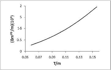
Figure 1: $\frac{\delta m^{(2)}}{m}$ vs $T/m$ for $T<m,$ for two loop one particle irreducible diagrams.

The temperatures of particular interest during BBN are $0.08$ MeV $\lesssim T\lesssim 0.03$ MeV, since most of the Helium produced, was synthesized during this range of temperature. Two loop correction at temperature $T<m,$ from one particle irreducible diagrams, the value of $\Delta Y$ is $3.20\times 10^{-5}$. A similar situation was found while determining these ratios for one loop corrections in ref. Saleem1987 . This value remains constant here since the $T/m$ dependence cancels out in the two loop correction to expression for $\Delta Y,$ for low temperatures, as can be seen from eqs. (4) and (6). It is evident that the two loop corrections at temperature $T<m$ though small, are not completely negligible. The corrections to $\Delta Y$ obtained here are in the fifth decimal places. The behavior of $\frac{\delta m^{(2)}}{m},$ with change in $T/m$ for the temperature range $0.08$ MeV $\lesssim T\lesssim 0.03$ MeV is plotted in figure 1. The variation in $\frac{\delta m^{(2)}}{m},$ with change in $T/m$ for this temperature range comes out to be between $2.75\times 10^{-6}$ and $1.96\times 10^{-5}.$

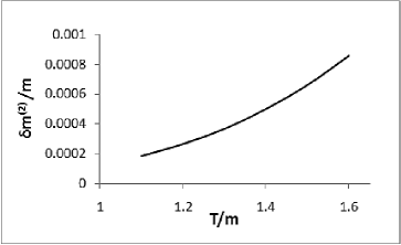
Figure 2: $\frac{\delta m^{(2)}}{m}$ vs $T/m$ for $T>m,$ for two loop one particle irreducible diagrams.

Using eq. (2), the variation in $\frac{\delta m^{(2)}}{m},$ with change in $T/m$ for the temperature range relevant in QED soon after the freezeout of weak interactions, is between $1.8\times 10^{-4}$ and $8.6\times 10^{-4}.$ This variation in $\frac{\delta m^{(2)}}{m}$ vs $T/m$ for $T>m$ in this temperature range is plotted in figure 2, for two loop one particle irreducible diagrams.

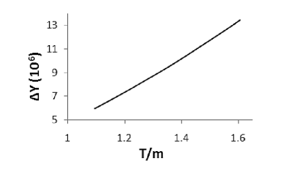
Figure 3: $\Delta Y$ vs $T/m$ for $T>m,$ for two loop one particle irreducible diagrams for $0.82$ MeV $\lesssim T\lesssim 0.56$ MeV.

The plot of $\Delta Y$ vs $T/m$ for temperatures $0.82$ MeV $\lesssim T\lesssim 0.56$ MeV, is given in figure 3. The values of $\Delta Y$ vary between $1.35\times 10^{-5}$ and $5.95\times 10^{-6}$. These values are somewhat smaller at $T>m$ probably due to the reason that even the synthesis of light elements was not much as compared to this synthesis during the range of temperature $0.08$ MeV $\lesssim T\lesssim 0.03$ MeV, when there was sudden burst of light elements nucleosynthesis. The values of $\Delta Y$ obtained for two loops are significantly smaller than $\Delta Y$ values with one loop corrections. This is in accordance with the perturbative nature of QED. It needs to be mentioned that from eq. (3), the value of $\Delta Y\thicksim 4.15\times$ $10^{-6}$ at $T$ $\thicksim$ $m$, (energies $\thicksim 0.5\$MeV).

Other parameters such as the relative change in the neutrino temperature

$$\frac{\Delta T_{\nu}}{T_{\nu}}=-0.1\left(\frac{m}{T}\right)^{2}\frac{\delta m}{m},$$

the change in neutrino temperature relative to photon temperature

$$\frac{\Delta T_{\nu}}{T}=-\left(\frac{m}{5T}\right)^{2}\frac{\delta m}{m},$$

and the relative variation in the total energy density of the universe during the era under consideration

$$\frac{\Delta\rho_{T}}{\rho_{T}}=-\left(\frac{m}{4T}\right)^{2}\frac{\delta m}{m}$$

are also calculated using Dicus1982 the expressions of two loop modifications to $\frac{\delta m}{m}$ for the relevant temperature limits in eqs. (2) - (5) for two loop irreducible diagrams. The values from these relations for $T>m$ are listed in Table 1.

$T$ (MeV)	$\frac{\delta m}{m}$	$\Delta Y$	$\frac{\Delta T_{\nu}}{T_{\nu}}$	$\frac{\Delta T_{\nu}}{T}$	$\frac{\Delta\lambda}{\lambda}$	$\frac{\Delta\rho_{T}}{\rho_{T}}$
$0.6$	$0.00024$	$6.96\times 10^{-6}$	$-1.74\times 10^{-5}$	$6.96\times 10^{-6}$	$-3.5\times 10^{-5}$	$1.09\times 10^{-5}$
$0.7$	$0.00046$	$9.71\times 10^{-6}$	$-2.43\times 10^{-5}$	$9.71\times 10^{-6}$	$-4.9\times 10^{-5}$	$1.52\times 10^{-5}$
$0.8$	$0.00078$	$1.28\times 10^{-5}$	$-3.19\times 10^{-5}$	$1.28\times 10^{-5}$	$-6.4\times 10^{-5}$	$2.0\times 10^{-5}$
$0.9$	$0.0013$	$1.62\times 10^{-5}$	$-4.06\times 10^{-5}$	$1.62\times 10^{-5}$	$-8.1\times 10^{-5}$	$2.54\times 10^{-5}$
$1.0$	$0.0019$	$2.01\times 10^{-5}$	$-5.02\times 10^{-5}$	$2.01\times 10^{-5}$	$-0.0001$	$3.14\times 10^{-5}$
$1.1$	$0.0028$	$2.43\times 10^{-5}$	$-6.08\times 10^{-5}$	$2.43\times 10^{-5}$	$-0.00012$	$3.80\times 10^{-5}$
$1.2$	$0.0039$	$2.9\times 10^{-5}$	$-7.24\times 10^{-5}$	$2.9\times 10^{-5}$	$-0.00014$	$4.52\times 10^{-5}$
$1.3$	$0.0055$	$3.4\times 10^{-5}$	$-8.49\times 10^{-5}$	$3.4\times 10^{-5}$	$-0.00017$	$5.31\times 10^{-5}$
$1.4$	$0.0074$	$3.9\times 10^{-5}$	$-9.85\times 10^{-5}$	$3.9\times 10^{-5}$	$-0.0002$	$6.16\times 10^{-5}$
$1.5$	$0.0097$	$4.5\times 10^{-5}$	$-0.00011$	$4.5\times 10^{-5}$	$-0.00023$	$7.07\times 10^{-5}$

Table 1. The values of $\Delta Y$, $\frac{\Delta T_{\nu}}{T}$, $\frac{\Delta\lambda}{\lambda}$, $\frac{\Delta\rho_{T}}{\rho_{T}}$, and $\frac{\Delta T_{\nu}}{T_{\nu}}$ obtained for temperature range $0.6$ MeV $\leq T\leq$ $1.5$ MeV.

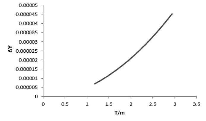
Figure 4: Plot of second order corrections to $\Delta Y$ vs $T/m$ for $0.6$ MeV $\leq T\leq$ $1.5$ MeV.

The values of $\Delta Y$, $\frac{\Delta T_{\nu}}{T}$, $\frac{\Delta\lambda}{\lambda}$, $\frac{\Delta\rho_{T}}{\rho_{T}}$, and $\frac{\Delta T_{\nu}}{T_{\nu}}$ obtained for $T>m$ in the temperature range $0.6$ MeV $\leq T\leq$ $1.5$ MeV are plotted vs $T/m$ in figures (4) - (8) respectively. In figure 4, the second order correction to $\Delta Y$ parameter is plotted vs $T/m$ . The values of $\Delta Y$ vary from $6.96\times 10^{-6}$ to $4.53\times 10^{-5}$ for the range of temperature $0.6$ MeV $\leq T\leq$ $1.5$ MeV.

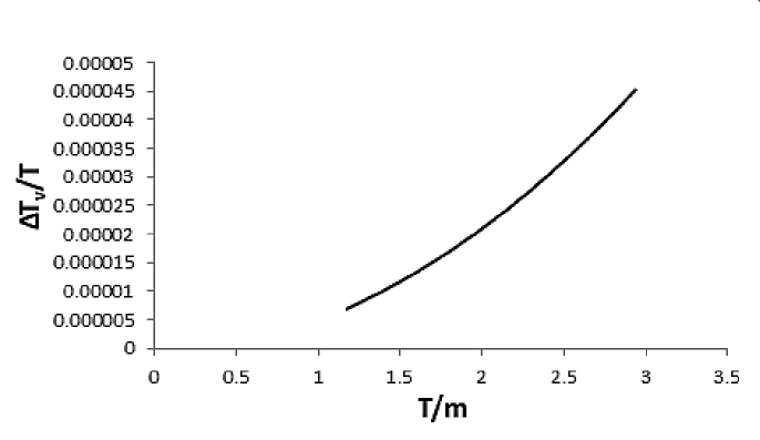
Figure 5: Plot of two loop corrections to $\frac{\Delta T_{\nu}}{T}$ vs $T/m$ for $T>m$.

As portrayed in figure 5 for $\frac{\Delta T_{\nu}}{T},$ the values show an increasing behavior with increase in $T/m$. Table 1 shows that as $T$ varies between $0.6$ MeV $\leq T\leq$ $1.5$ MeV, the values of $\frac{\Delta T_{\nu}}{T}$ increase from $6.96\times 10^{-6}$ to $4.53\times 10^{-5}.$

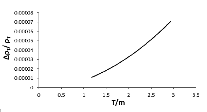
Figure 6: Plot of second order corrections to $\frac{\Delta\rho_{T}}{\rho_{T}}$ vs $T/m$ for $0.6$ MeV $\leq T\leq$ $1.5$ MeV.

Figure 6 also depicts an increase in the values of $\frac{\Delta\rho_{T}}{\rho_{T}}$ vs $T/m$. The range in variation of the values of $\frac{\Delta\rho_{T}}{\rho_{T}}$ is from $1.09\times 10^{-5}$ to $7.07\times 10^{-5}$ for $0.6$ MeV $\leq T\leq$ $1.5$ MeV, shown in Table 3. Figure 7 gives the variation of relative decay rate of neutrons $\frac{\Delta\lambda}{\lambda}$ with $T/m$ which is negative and varies from $-3.5\times 10^{-5}$ to $-2.3\times 10^{-4}$ for the same variation in temperature.

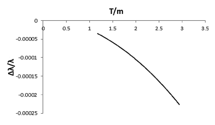
Figure 7: Plot of two loop corrections to $\frac{\Delta\lambda}{\lambda}$ vs $T/m$ for $T>m$.

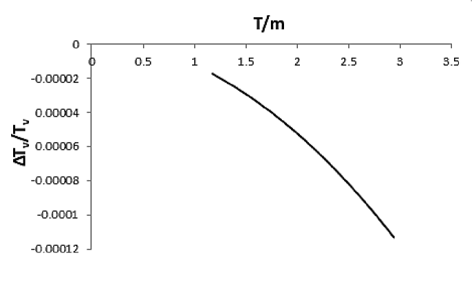
Figure 8: Plot of two loop corrections to $\frac{\Delta T_{\nu}}{T_{\nu}}$ vs $T/m$ for $T>m$.

Figure 8 is a plot for variation of $\frac{\Delta T_{\nu}}{T_{\nu}}$ from $-1.74\times 10^{-5}$ to $-1.13\times 10^{-4}$ for $0.6$ MeV $\leq T\leq$ $1.5$ MeV. The relative variations in all these parameters though small are not completely negligible.

The latest observational probes such as Planck, Herschel and James Webb Space Telescope are to provide further fine tuning in precision measurement for the values of these parameters. The finite temperature corrections around the electron mass scale are interesting since even up to second order in $\alpha,$ they give corrections within the recently measurable range of observational probes, within uncertainities. Higher order corrections to weak processes may be also interesting and useful for estimating modifications to parameters in the early universe, due to finite temperature effects.

Acknowledgement: The authors are thankful to Prof. Riazuddin and Samina S. Masood for useful discussions and suggestions. Higher Education Commission (HEC), Pakistan is acknowledged for partial funding under a research grant # 1925 during this work.

Figure Captions

Figure 1. $\frac{\delta m^{(2)}}{m}$ vs $T/m$ for $T<m,$ for two loop one particle irreducible diagrams.

Figure 2. $\frac{\delta m^{(2)}}{m}$ vs $T/m$ for $T>m,$ for two loop one particle irreducible diagrams.

Figure 3. $\Delta Y$ vs $T/m$ for two loop one particle irreducible diagrams for $0.82$ MeV $\lesssim T\lesssim 0.56$ MeV.

Figure 4. Plot of second order corrections to $\Delta Y$ vs $T/m$ for $0.6$ MeV $\leq T\leq$ $1.5$ MeV.

Figure 5. Plot of second order corrections to $\frac{\Delta T_{\nu}}{T}$ vs $T/m$ for $0.6$ MeV $\leq T\leq$ $1.5$ MeV.

Figure 6. Plot of two loop corrections to$\ \frac{\Delta\rho_{T}}{\rho_{T}}$ vs $T/m$ for $T>m$.

Figure 7. Plot of second order corrections to$\ \frac{\Delta\lambda}{\lambda}$ vs $T/m$ for $T>m$.

Figure 8. Plot of two loop corrections to $\frac{\Delta T_{\nu}}{T_{\nu}}$ vs $T/m$ for $T>m$.

References

- (1) S. Weinberg, Gravitation and Cosmology, John Wiley & Sons (2004); E. W. Kolb and M. S. Turner, The Early Universe, Addison Wesley, (1990); A. R. Liddle and J. Loveday, The Oxford Companion to Cosmology, University Press, Oxford (2008).
- (2) G. Hinshaw et. al, Five-year Wilkinson Microwave Anisotropy Probe (WMAP) observations: Data processing, sky maps, and basic results, Astrophys. J. Suppl. 180 (2009) 225-245.
- (3) R. A. Alpher, H. Bethe, and G. Gamow, The origin of chemical elements, Phys. Rev. 73 (1948) 803-804; R. A. Alpher, R. C. Herman, Theory of the origin and relative abundance distribution of the elements, Rev. Mod. Phys. 22 (1950) 153-212.
- (4) C. L. Bennett et. al, Seven-year Wilkinson Microwave Anisotropy Probe (WMAP) observations: Are there cosmic microwave background anomalies? Astrophys. J. Suppl. 192 (2011) 17-35.
- (5) Richard H. Cyburt, Brian D. Fields, and Keith A. Olive, Primordial nucleosynthesis in light of WMAP, Phys. Lett. B567 (2003) 227-234.
- (6) Alain Coc, Elisabeth Vangioni-Flam, Pierre Descouvemont, Abderrahim Adahchour, and Carmen Angulo, Updated Big-Bang nucleosynthesis compared to WMAP results, AIP Conf. Proc. 704 (2004) 341-350.
- (7) G. Steigman, Primordial Nucleosynthesis after WMAP, Chemical abundances in the universe: Connecting first stars to planets, in Proc. IAU Sympos. No. 265, edited by K. Kunha et al. (2009).
- (8) Ann Merchant Boesgaard and Gary Steigman, Big Bang Nucleosynthesis: Theories and observations, Ann. Rev. Astron. Astrophys. 23 (1985) 319-378.
- (9) Jong-Mann Yang, Michael S. Turner, G. Steigman, D. N. Schramm, and Keith A. Olive, Primordial Nucleosynthesis: A critical comparison of theory and observation, Astrophys. J. 281 (1984) 493-511.
- (10) Keith A. Olive, Gary Steigman, and Terry P. Walker, Primordial nucleosynthesis: Theory and observations, Phys. Rep. 333 (2000) 389-407.
- (11) Keith A. Olive, David N. Schramm, Gary Steigman, Michael S. Turner, and Jong-Mann Yang, Big Bang Nucleosynthesis as a probe of cosmology and particle physics, Astrophys. J. 246 (1981) 557-568.
- (12) Gary Steigman, Primordial Nucleosynthesis: The predicted and observed abundances and their consequences, in Proceedings of the 11th Symposium on Nuclei in the Cosmos (NIC ’11), N. Christlieb, Ed., PoS, Trieste, Italy (2010).
- (13) G. Steigman, Primordial Nucleosynthesis: Successes and challenges, Int. J. Mod. Phys. E15 (2006) 1-36.
- (14) G. Steigman, Primordial Nucleosynthesis in the precision cosmology era, Annu. Rev. Nucl. Part. Sci. 57 (2007) 463-491.
- (15) G. Miele and O. Pisanti, Primordial Nucleosynthesis: an updated comparison of observational light nuclei abundances with theoretical predictions, Nucl. Phys. B (Proc. Suppl.) 188 (2009) 15-19.
- (16) A. Coc and E. Vangioni, Big-Bang nucleosynthesis with updated nuclear data, J. Phys.: Conf. Series, 202 (2010) 012001.
- (17) Gary Steigman, Primordial Helium and the Cosmic Background Radiation, JCAP 1004 (2010) 029-037.
- (18) Keith A. Olive, Evan Skillman, and Gary Steigman, The Primordial abundance of He-4: An Update, Astrophys. J. 483 (1997) 788-797.
- (19) Gary Steigman, Big bang nucleosynthesis, Nucl. Phys. Proc. Suppl. 48 (1996) 499-507.
- (20) N. Hata, R. J. Scherrer, G. Steigman, D. Thomas, T. P. Walker, Sidney A. Bludman, and P. Langacker, Big bang nucleosynthesis in crisis, Phys. Rev. Lett. 75 (1995) 3977-3980.
- (21) M. J. Balbes, R. N. Boyd, and G. Steigman, D. Thomas, Post big bang processing of the primordial elements, Astrophys. J. 459 (1996) 480-498.
- (22) Keith A. Olive and Gary Steigman, On the abundance of primordial helium, Astrophys. J. Suppl. 97 (1995) 49-58.
- (23) Gary Steigman, Big bang nucleosynthesis comes of age, Phys. Scripta T36 (1991) 55-59.
- (24) Keith A. Olive, David N. Schramm, Gary Steigman, and Terry P. Walker, Big Bang Nucleosynthesis Revisited, Phys. Lett. B236 (1990) 454–460.
- (25) Gary Steigman, Primordial Nucleosynthesis: A Window On The Early Universe, Nucl. Phys. B252 (1985) 11-24.
- (26) Dana S. Balser, The Chemical Evolution of Helium, Astron. J. 132 (2006) 2326-2332.
- (27) Brian Fields and Subir Sarkar, Big-Bang nucleosynthesis, J. Phys. G33 (2006) 1-1232.
- (28) Richard H. Cyburt, Primordial nucleosynthesis in the new cosmology, Nucl. Phys. A718 (2003) 380-382.
- (29) Gary Steigman, Big bang nucleosynthesis, Nucl. Phys. Proc. Suppl. 37C (1995) 68-73.
- (30) Terry P. Walker, Gary Steigman, David N. Schramm, Keith A. Olive, and Ho-Shik Kang, Primordial nucleosynthesis redux, Astrophys. J. 376 (1991) 51-69.
- (31) George M. Fuller and Christel J. Smith, Nuclear weak interaction rates in primordial nucleosynthesis, Phys. Rev. D82 (2010) 125017-1 -125017-9.
- (32) Sourish Dutta and Robert J. Scherrer, Big Bang nucleosynthesis with a stiff fluid, Phys. Rev. D82 (2010) 083501-1 - 083501-5.
- (33) Erik Aver, Keith A. Olive, and Evan D. Skillman, A New Approach to Systematic Uncertainties and Self-Consistency in Helium Abundance Determinations, JCAP 1005 (2010) 003-053.
- (34) Manuel Peimbert, The Primordial Helium Abundance, Curr. Sci. 95 (2008) 1165-1176.
- (35) Fabio Iocco, Gianpiero Mangano, Gennaro Miele, Ofelia Pisanti, and Pasquale D. Serpico, Primordial Nucleosynthesis: from precision cosmology to fundamental physics, Phys. Rep. 472 (2009) 1-76.
- (36) Thomas Dent, Steffen Stern, Christof Wetterich, Big Bang nucleosynthesis as a probe of fundamental constants, J. Phys. G35 (2008) 014005-1 - 014005-6.
- (37) Ruben Salvaterra, A. Ferrara, Is primordial He truly from big bang? Mon. Not. Roy. Astron. Soc. 340 (2003) L17-L20.
- (38) David Tytler, John M. O’Meara, Nao Suzuki, Dan Lubin, Review of Big Bang nucleosynthesis and primordial abundances, Phys. Scripta T85 (2000) 12-31.
- (39) S. Esposito, G. Mangano, G. Miele, O. Pisanti, Big bang nucleosynthesis: An accurate determination of light element yields, Nucl. Phys. B568 (2000) 421-444.
- (40) Peter J. Kernan and Subir Sarkar, No crisis for big bang nucleosynthesis, Phys. Rev. D54 (1996) 3681-3685.
- (41) Brian D. Fields, On the evolution of the light elements D, He-3, and He-4, Astrophys. J. 456 (1996) 478-498.
- (42) Brian D. Fields, Kimmo Kainulainen, Keith A. Olive, and David Thomas, Model independent predictions of big bang nucleosynthesis from He-4 and Li-7: Consistency and implications, New Astron. 1 (1996) 77-96.
- (43) D. A. Dicus, E. W. Kolb, A. M. Gleeson, E. C. G. Sudarshan, V. L. Teplitz, and M. S. Turner, Primordial Nucleosynthesis including radiative, Coulomb, and finite temperature corrections to weak rates, Phys. Rev. D26 (1982) 2694-2706.
- (44) A. E. I. Johansson, G. Peressutti, B. S. Skagerstam, Quantum field theory at finite temperature: Renormalization and radiative corrections, Nucl. Phys. B278 (1986) 324-342.
- (45) G. Peressutti, B. S. Skagerstam, Finite temperature effects in quantum field theory, Phys. Lett. B110 (1982) 406-410.
- (46) L. Cambier, J. Primack, and M. Sher, Finite temperature radiative corrections to neutron decay and related processes, Nucl. Phys. B209 (1982) 372-388.
- (47) D. Bailin and A. Love, Cosmology in Gauge Field Theory and String Theory, IoP Pub. Ltd., Bristol and Philadelphia (2004).
- (48) H. Hecht, The electron-neutrino cross-section and its effect on the cosmological helium abundance, Astrophys. J. 170 (1971) 401-404.
- (49) M. Schwarzchild, Structure and Evolution of the Stars Structure, ed. by L. H. Aller and D. B. Mclaughlin, University of Chicago Press, Princeton (1958).
- (50) J. N. Bahcall, W. A. Fowler, I. Iben Jr., and R. L. Sears, Solar neutrino flux, Astrophys. J. 137 (1963) 344-346.
- (51) R. L. Sears, Helium content and neutrino fluxes in solar models, Astrophys. J. 140 (1964) 477-484.
- (52) I. J. Danziger, The cosmic abundance of helium, Ann. Rev. Astron. and Astrophys. 8 (1970) 161-178.
- (53) D. N. Spergel et. al, Wilkinson Microwave Anisotropy Probe (WMAP) Three Year Observations: Implications for Cosmology, Astrophys. J. Suppl. 170 (2007) 377-408.
- (54) K. A. Olive and E. Skillman, A Realistic Determination of the Error on the Primordial Helium Abundance, Astrophys. J. 617 (2004) 29-49.
- (55) Y. I. Izotov et. al, The primordial abundance of He: a self-consistent empirical analysis of systematic effects in a large sample of low-metallicity HII regions, Astrophys. J. 662 (2007) 15-38.
- (56) M. Peimbert et. al, Revised Primordial helium abundance derived from new atomic data, Astrophys. J. 666 (2007) 636-646.
- (57) E. J. Levinson and D. H. Boal, Self-energy corrections to fermions in the presence of a thermal background, Phys. Rev. D31 (1985) 3280-3284.
- (58) D. A. Dicus, D. Down, and E. W. Kolb, On perturbation theory at finite temperature, Nucl. Phys. B223 (1983) 525-531.
- (59) S. Saleem, Finite-temperature and -density effects on electron self-mass and primordial nucleosynthesis, Phys. Rev. D36 (1987) 2602-2605.
- (60) J. F. Donoghue and B. R. Holstein, Quantum electrodynamics at finite temperature, Phys. Rev. D28 (1983) 340; [Erratum ibid 29 (1983) 3004].
- (61) J. F. Donoghue, B. R. Holstein, and R. W. Robinett, Quantum electrodynamics at finite temperature, Ann. Phys. (N.Y.) 164 (1985) 233-253.
- (62) Samina S. Masood, Photon mass in the classical limit of finite-temperature and -density QED, Phys. Rev. D44 (1991) 3943-3948.
- (63) K. Ahmed and Samina Saleem, Renormalization and radiative corrections at finite-temperature reexamined, Phys. Rev. D35 (1987) 1861-1871.
- (64) K. Ahmed and Samina Saleem, Vacuum polarization at finite temperature and density in QED, Ann. Phys. (N.Y.) 207 (1991) 460-473.
- (65) K. Ahmed and Samina S. Masood, Finite-temperature and -density renormalization effects in QED, Phys. Rev. D35 (1987) 4020-4023.
- (66) Samina S. Masood and Mahnaz Q. Haseeb, Gluon polarization at finite temperature and density, Astropart. Phys. 3 (1995) 405-412.
- (67) Samina S. Masood and Mahnaz Qader, Finite-temperature and -density corrections to electroweak processes, Phys. Rev. D46 (1992) 5110-5116.
- (68) Mahnaz Qader, Samina S. Masood, and K. Ahmed, Second-order electron mass dispersion relation at finite temperature, Phys. Rev. D44 (1991) 3322-3327.
- (69) Samina S. Masood, and Mahnaz Q. Haseeb, Second-order corrections to QED coupling at low temperature, Int. J. of Mod. Phys. A23 (2008) 4709-4719.
- (70) Mahnaz Q. Haseeb and Samina S. Masood, Two loop low temperature corrections to electron self energy, Chin. Phys. C35 (2010) 608-611.
- (71) Mahnaz Qader, Samina S. Masood, and K. Ahmed, Second-order electron mass dispersion relation at finite temperature. II., Phys. Rev. D46 (1992) 5633-5647.
- (72) Mahnaz Q. Haseeb and S. S. Masood, Second order thermal corrections to electron wavefunction, Phys. Lett. B704 (2011) 66-73.
- (73) Samina S. Masood and Mahnaz Q. Haseeb, Second-order corrections to the magnetic moment of electron at finite temperature, Int. J. of Mod. Phys. A27 (2012) 1250188-1250197.