Quantum energy decays and decoherence in discrete baths

Abstract

The quantum average energy decay and the purity decay are studied for a system particle as a function of the number of constituents of a discrete bath model. The system particle is subjected to two distinct physical situations: the harmonic oscillator (HO) and the Morse potential. The environment (bath) is composed by a finite number $N$ of uncoupled HOs, characterizing the structured bath, which in the limit $N\to\infty$ is assumed to have an ohmic, sub-ohmic or super-ohmic spectral density. For very low values of $N$ the mean energy and purity remain constant in time but starts to decay for intermediate values ($10\lesssim N\lesssim 20$), where two distinct time regimes are observed: two exponential decays for relatively short times and a power-law decay for larger times. In this interval of $N$ decoherence occurs for short times and a non-Markovian dynamics is expected for larger times. When $N$ increases, energy and coherence decay very fast and a Markovian dynamics is expected to occur. Wave packet dynamics is used to determine the evolution of the particle inside the system potentials.

1 Introduction

The quantum dissipation and decoherence are analyzed here for an open system interacting with its environment by collision processes. The problem (System+Environment+Interaction) is conservative but, due to energy exchange between system and environment, the system can be seen as an open system with dissipation. Such theoretical model has been proposed and studied in quantum [1, 2, 3] and classical [2, 3, 4] systems. Various models were developed to treat such open system. We start by mention the methods which have focused on an explicit quantum dynamical treatment of the system+bath dynamics: the multiconfiguration time-dependent Hartree (MCTDH) technique for wave packet propagation [5], the Gaussian-MCTDH approach [6], the effective-mode representation[7], and the local coherent-state approximation to system-bath dynamics [8]. Another way of studying the system+bath dynamics is to solve the non-Markovian master equations [9, 10], including some semiclassical approaches [11, 12, 13].

Here a non-Markovian quantum trajectory theory is used, named non-Markovian quantum-state diffusion, that describes the dynamics of a quantum system coupled linearly via position to a environment [14, 15, 16, 17]. Differently from most the previous studies, the environment is composed by a finite number, $N$, of uncoupled HOs, as studied before for classical systems [18, 19]. In such cases we say to have a discrete or structured bath. Structured baths have become important since they describe realistic physical situations of non-equilibrium physics. One major recent application is the energy transfer between a light-harvesting protein and a reaction center protein [20]. Understanding the physics encountered in this process will help exploring its huge potential [21]. Some experiments in which the non-Markovian behavior arises due to the discreteness of the bath can be mentioned: high-Q microwave cavities, quantum optics in materials with a photonic band gap, output coupling from a Bose-Einstein condensate to create an atom laser [22, 23, 24, 25, 26] or the decoherence phenomenon [27, 28, 29, 30]. From the classical point of view, in the context of finite baths with uncoupled HO, there are some works which analyze the effect of discrete (structured) baths on the system energy decay [4, 18, 19]. The main result found is that finite baths may induce a non-Markovian dynamics on the system particle. From the quantum point of view, most works [4, 6, 8, 13, 30, 31] focus on the analysis of changing the frequencies distribution and the coupling strength between system and bath.

We analyze systematically the effect of increasing the number of oscillators $N$ from the bath on the system energy decay. In most cases we vary $N=1\to 100$. As $N$ increases, the quantum simulations, usually done here for $500$ realizations of the bath, need very long computational times. For very low values of $N$ the mean time energy decay keeps constant but starts to decay for intermediate values of $N$. For $10\leq N\leq 50$ a transition to exponential decay for shorter times and a power-law decay for larger times is observed. For higher values $N>100$ only exponential decay is observed. In the interval $20\leq N\leq 50$ an additional power-law decay between the two previously mentioned behaviors is observed.

The paper is organized as follows. In Section 2 we introduce the basic concepts of non-Markovian quantum-state diffusion and derive a new simplified stochastic Schrödinger equation valid for finite baths. In Section 3 the simplified equation is applied to analyze the $N$ dependence of some useful physical quantities such as the energy decay, the average position, and the purity (decoherence). In this section harmonic potential is considered. In Section 4 a Morse potential is used for the system particle. In the last section we present a summary and the conclusions.

2 Linear non-Markovian quantum-state diffusion

The non-Markovian quantum-state diffusion (QSD) equation is based on a standard model of open system dynamics: a quantum system interacting with a bosonic environment with the total Hamiltonian

$$H_{tot}=H+\sum_{\lambda}g_{\lambda}(La^{+}_{\lambda}+L^{+}a_{\lambda})+\hbar\sum_{\lambda}\omega_{\lambda}a^{+}_{\lambda}a_{\lambda},$$ (1)

where $H$ is the Hamiltonian of the system of interest, $L$ is a system operator coupling to environment and $a^{+}_{\lambda}$, $a_{\lambda}$ are the raising and lowering operators, with the property $[a_{\lambda},a^{+}_{\lambda^{{}^{\prime}}}]=\delta_{\lambda\lambda^{{}^{\prime}}}$. The linear non-Markovian QSD equation [16, 17, 34, 35, 36] is given by

$$\hbar\left|\dot{\psi}_{t}\right>=-iH^{\prime}\left|\psi_{t}\right>+Lz^{*}_{t}\left|\psi_{t}\right>-L^{+}\int^{t}_{0}dsK(t-s)\frac{\delta\left|\psi_{t}\right>}{\delta z^{*}_{s}},$$ (2)

where was assumed a factorized total initial state $\left|\psi_{0}\right>\left|0_{1}\right>\left|0_{2}\right>\cdots\left|0_{\lambda}\right>\cdots$, with an arbitrary system state $\left|\psi_{0}\right>$ and all environmental oscillators in their ground state $\left|0_{\lambda}\right>$.

$$z^{*}_{t}=-i\sum_{\lambda}g^{*}_{\lambda}z^{*}_{\lambda}e^{i\omega_{\lambda}t}$$ (3)

is a complex Gaussian process with zero mean and correlations $M[z^{*}_{t}z_{s}]=K(t-s)=\sum_{\lambda}|g_{\lambda}|^{2}e^{-i\omega_{\lambda}(t-s)}$, where $M[]$ denotes the ensemble average over the classical driving noise. The form of $K(t-s)$ corresponds to the zero-temperature limit. $\lambda$ is the number of oscillators from the bath, $g_{\lambda}$ is the coupling to oscillator $\lambda$, $\omega_{\lambda}$ is its frequency and $z^{*}_{\lambda}=(x_{\lambda}+iy_{\lambda})/\sqrt{2}$, where $(x_{\lambda},y_{\lambda})$ are normal (Gaussian) distributed real number with zero mean and deviation one. The many realizations to solve the stochastic Schrödinger equation are done over these normal distributed numbers. The functional derivative of equation (2) can be written in the first order approximation as a linear function of $\left|\psi_{t}\right>$

$$\frac{\delta\left|\psi_{t}\right>}{\delta z^{*}_{s}}=O(t,s,z^{*})\left|\psi_{t}\right>=e^{-iH(t-s)}Le^{iH(t-s)}\left|\psi_{t}\right>.$$ (4)

Now, taking $L=L^{+}=q$, which is the position operator from the system, the stochastic Schrödinger equation becomes

$$\hbar\left|\dot{\psi}_{t}\right>=-iH^{\prime}\left|\psi_{t}\right>+qz^{*}_{t}\left|\psi_{t}\right>-q\int^{t}_{0}dsK(t-s)e^{-iH(t-s)}qe^{iH(t-s)}\left|\psi_{t}\right>.$$ (5)

In equation (2) and (5), the Hamiltonian $H^{\prime}=H(q,p)+q^{2}A(t)$, with $A(t)=\sum_{\lambda}\frac{|g_{\lambda}|^{2}}{\omega_{\lambda}}(\cos\omega_{\lambda}t-1)$, contains an additional potential term that turns out to be counterbalanced by a similar term arising from the memory integral [35]. Our approach is consistent with the Redfield theory [37] in the long-time limit when $\int_{0}^{t}$ is replaced by $\int_{0}^{\infty}$.

Using $\left|\psi_{t}\right>=\sum_{n}c_{n}(t)\left|\phi_{n}\right>$, $H\left|\phi_{n}\right>=\epsilon_{n}\left|\phi_{n}\right>$, $q=\sum_{n,m}q_{nm}\left|\phi_{n}\right><\phi_{m}|$, and orthonormal condition $<\phi_{n}|\phi_{n^{\prime}}>=\delta_{nn^{\prime}}$, equation (5) transforms to

$$\hbar\dot{c}_{n}(t) = -i\epsilon_{n}c_{n}(t)-iA(t)\sum_{mm^{\prime}}q_{nm}q_{mm^{\prime}}c_{m^{\prime}}(t)+z^{*}_{t}\sum_{m}q_{nm}c_{m}(t)$$ (8)

$$-\sum_{m,m^{\prime}}q_{nm^{\prime}}\bar{O}_{mm^{\prime}}(t)c_{m^{\prime}}(t),$$

where

$$\bar{O}_{mm^{\prime}}(t)=<\phi_{m}|\bar{O}(t)\left|\phi_{m^{\prime}}\right>=q_{mm^{\prime}}\sum_{\lambda}|g_{\lambda}|^{2}\frac{e^{-i[\omega_{\lambda}+(\epsilon_{m}-\epsilon_{m^{\prime}})]t}-1}{-i[\omega_{\lambda}+(\epsilon_{m}-\epsilon_{m^{\prime}})]},$$ (9)

and

$$\bar{O}(t)=\int^{t}_{0}dsK(t-s)e^{-iH(t-s)}qe^{iH(t-s)}.$$ (10)

For simplicity, we choose the Planck constant $\hbar=1$ throughout the paper. At next we analyze the following quantities: The quantum average of the system energy which is given by

$$\left<E\right>=\left<\psi_{t}|H|\psi_{t}\right>=\sum_{n}c_{n}^{*}(t)c_{n}(t)\epsilon_{n},$$ (11)

and the quantum average of the system position

$$\left<q\right>_{t}=\left<\psi_{t}\right|q\left|\psi_{t}\right>=\sum_{n,m}c_{n}^{*}(t)c_{m}(t)q_{nm},$$ (12)

and finally the purity which gives informations about the decoherence occurred in the system [13]:

$$P=\mbox{Tr}_{c}\left[\rho_{s}^{2}(t)\right]=\sum_{nm}M[c_{n}c_{m}^{*}]M[c_{m}c_{n}^{*}],$$ (13)

where $\rho_{s}(t)=M\left[\left|\psi_{t}\right>\left<\psi_{t}\right|\right]$ is the reduced density matrix.

Now the stochastic Schrödinger equation coupled to a finite bath, Eq. (8), will be implemented to calculate the energy decay, mean position and purity for the system particle inside two types of potentials, widely used in physics: the harmonic potential and the Morse potential. We also consider the time evolution of the quantum average position.

3 Harmonic potential coupled to $N$ oscillators

In this section we consider a particle inside a harmonic potential coupled to a discrete bath of $N$ HOs. This problem has exact solutions [2] which can be used to compare some quantities calculated with the approach used here. The frequencies $\omega_{\lambda}$ are distributed in the interval $(1.1,2.1)$ and are picked randomly from a frequencies generator, but once picked they will be kept fixed during the simulations, even for different bath realizations. In this approach, due to the finite number of HOs in the bath, the spectral density is determined numerically and is always structured for low values of $N$ (see [18] for more details in the classical case). The properties of the bath depend on the frequency’s distribution of the $N$ HOs [18]. In the limit $N\to\infty$ we assume to have three distinct continuous distributions: ohmic bath (quadratic), sub-ohmic and super-ohmic. Each oscillator will have a distinct $(x_{\lambda},y_{\lambda})$ pair, randomly chosen numbers with zero mean and deviation one. For each coefficient $c_{n}$ of Eq. (8) we consider a rectangular initial conditions: $c_{n}(0)=1+0\cdot i$, with $n=1,\dots,n_{max}$, where $n_{max}$ is the last energy level considered. The first $n_{max}=15$ energy’s levels from the harmonic potential are considered, with energy $E_{n}=\hbar\omega(n-\frac{1}{2})$. Using $\omega=\hbar=1.0$ the ground state energy level equals $0.5$. Thus our initial state is given by

$$\left|\psi_{0}\right>=\frac{1}{\sqrt{n_{max}}}\sum_{n=1}^{n_{max}=15}\left|\phi_{n}\right>,$$ (14)

which is an entanglement of all $15$ system levels. In order to obtain the energy time decay and the average position as a function of the number of oscillators in the bath, Eq. (8) is integrated by a fourth-order Runge-Kutta integrator [38] and the values of $c_{n}(t)$ are introduced in Eqs. (11) and (12).

In the first part of this section the frequencies of the harmonic oscillators from the bath will follow a quadratic distribution, making the spectral density to be linear $J(\omega\leq\omega_{cut})\propto\omega$ when $N\to\infty$. $500$ initial conditions for the pairs $(x_{\lambda},y_{\lambda})$ will be considered for all the studied cases. To render the comparison easier the coupling strength will be kept constant, namely $g_{\lambda}=0.01$.

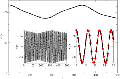
Figure 1: The average energy of a system, Eq. (11), coupled to a bath of one HO, with the coupling strength $g=0.01$. The two insets show the corresponding average positions, Eq.(12), for larger (left) and smaller (right) times. For comparison the circles (right) show exact results obtained from [2].

In Figure 1 the time evolution of the average energy $\left<E\right>$, Eq. (11), is plotted for a bath containing one harmonic oscillator with the frequency $\omega=2.09$. As inset graph is displayed the average position $\left<q\right>$ from Eq. (12). One can clearly see that for times $t_{d}\sim 170$ the system loses around $20\%$ of its initial energy for the bath, but is able to regain it at a later time $t_{R}\sim 320$. This exchange of energy between system and environment will repeat itself, with frequency around $\omega\sim 0.037$, for all integrated times (we checked it until $t=5000$). Thus, the mean energy over the return times (where the energy transferred into the bath returns to the system) is almost constant.

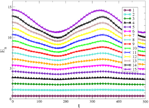
Figure 2: (Color online) The time evolution of all $15$ energy levels $E_{n}|c_{n}(t)|^{2}$

of a system coupled to a bath of one HO.

The return times of the energy are strongly dependent on the frequency of the bath oscillator but independent of the coupling intensity. This was checked for many coupling intensities. The time behavior of the energy was also confirmed by the time evolution of the average position: the system symmetrically oscillates very fast around the center $\left<q\right>=0$, with an amplitude which follows the pattern of energy decay. Namely, the minimum of the energy corresponds to the minimum of the highest amplitude. Figure 2 shows the time evolution of all the $15$ individuals energy levels $E_{n}|c_{n}(t)|^{2}$ of the harmonic potential for the same bath used in Fig. 1. Numbers denote the energy quantum number $n$. One can clearly notice that while the lowest states remain practically unchanged, the higher energy levels oscillate following the energy exchange observed in Fig. 1. Thus only the highest states are responsible for the energy exchange.

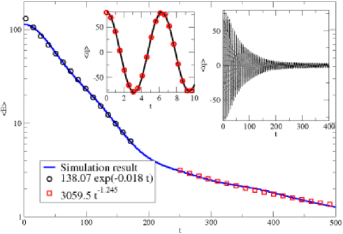
Figure 3: (Color online) The average energy decay, Eq. (11), for a bath of $10$ HOs, with the coupling strength equals to $0.01$. By symbols we display the best fits. The two insets show the corresponding average positions, Eq.(12), for larger (right) and smaller (left) times. For comparison the circles in the left inset show exact results obtained from [2].

In Figure 3 the energy decay is shown in a semi-log plot for a bath of $N=10$ HOs. In the time limit studied here ($t_{max}=500$) one can clearly see that the system energy will not be regained so that the time average from the system energy is not constant anymore. However, we expect that for some later times $t>t_{max}$ the energy will return to the system, since it is a finite system. The qualitative behavior of the energy decay rate changes for different time intervals. We show by symbols the best fits of the energy decay, namely an exponential fit, $\alpha=0.018$, for short times where a Markovian dynamics is expected and a power-law fit, $\beta=1.245$, for large times, where a non-Markovian dynamics occurs. We say that the qualitative change from exponential to power-law decay occurs close to times $t_{\alpha\to\beta}$. As inset graph we display the corresponding average position.

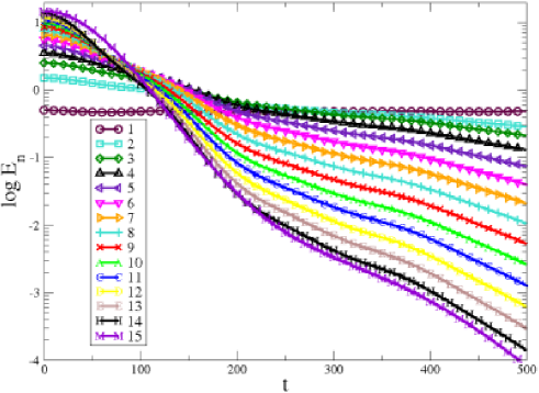
Figure 4: The time evolution of all $15$ energy levels $E_{n}|c_{n}(t)|^{2}$ of a system coupled to a bath containing $N=10$ HOs.

The time evolution of all the $15$ energy levels $E_{n}$ of a system coupled to a bath which has $N=10$ HOs is displayed in the semi-log plot of Fig. 4. Again it is clear that the higher energy levels decay faster. Something similar was shown to occur with the decoherence rate which is correlated to the highest occupied states [33]. In the long times region the energy levels are totally inverted: the highest energy level becomes the smallest one while the ground state energy becomes the most predominant one, followed by the second energy level and so on. By comparison with Fig. 3 we observe that the energy levels start to be totally inverted for times close to $250$, i. e. $t_{\alpha\to\beta}$ where the transition from exponential to power-law decay occurs. At these times it can be observed in Fig. 4 that the decay ratio $dE_{n}/dt$ decreases, meaning that the energy inserted in the bath starts to influence back the system dynamics, generating the non-Markovian behavior and the observed power law decay.

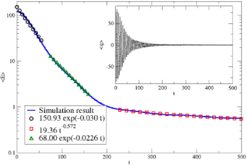
Figure 5: The average energy and its best fits for a bath of $N=20$ harmonic oscillators. As inset we shown the average position.

The energy decay and the average position for a bath of $N=20$ harmonic oscillators is displayed in Fig.  5. The system continues to behave dissipatively for the integrated time, with an exponential decay, $\left<E\right>\propto\exp(-0.030t)$ for $0<t\lesssim 50$ and a power-law decay $\left<E\right>\propto t^{-0.572}$ for much larger times $t\gtrsim 230$. For an intermediate time region, starting at $t\sim 75$ and ending at $t\sim 190$, an additional exponential decay, $\left<E\right>\propto\exp(-0.0226t)$, was observed. Such kind of behaviors with two exponential decays was encountered until $N\sim 50$ and completely disappeared for $N\geq 100$. By keeping the same line of arguments of Fig. 4 we can say that, for a bath of $20\leq N\leq 50$, the total inversion of the energy levels in times induces a power-law decay and the non-Markovian behavior.

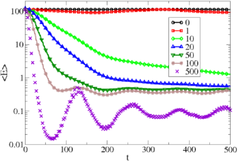
Figure 6: The energy decay for a bath with $N=1,10,20,50,100,500$ HOs. For $N=10,20,50$ we observe exponential and power-law decays.

In Figure 6 we summarize results of the energy decay for $N=1,10,20,50,100,$ $500$ HOs. The first observation is that the energy decays faster for larger $N$. For values $N=10,20,50$ we observe an exponential decay for shorter times and power-law decay for larger times. Details of the decay exponents will be discussed later in Figs. 9 and 10. As $N$ increases the time interval of power-law decay decreases and vanishes totally for $N=100$. Therefore, a non-Markovian motion is expected only for intermediate values of $N$. For $N\gtrsim 50$ a fluctuating behavior is observed and will be explained below.

Instead of looking at the dissipation, it is also possible to analyze the purity from Eq. (13) which gives informations about the decoherence occurred in the system. For our initial entangled state from Eq. (14), the initial reduced density matrix $\rho_{s}(0)$ has $15$ diagonal terms and $210$ off-diagonal terms. The off-diagonal terms are characteristic of the quantum coherence. Total decoherence of the initial state occurs at times $t_{dec}$ when all off-diagonal terms vanish. For these times a statistical mixture of the $15$ diagonal terms is reached and the the purity of the reduced density matrix is $P(t_{dec})=1/15\sim 0.067$. In this way it is possible to compare total decoherence times $t_{dec}$ with dissipation times.

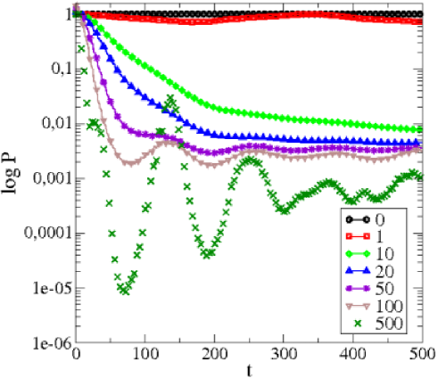
Figure 7: The purity for a bath with $N=1,10,20,50,100,500$ HOs.

In Fig. 7 we plot the time evolution of the purity, Eq. (13), for the same parameters shown in Fig. 6. For $N=0$ (no bath) the purity keeps constant to $1$. For $N=1$ the purity diminishes and increases a small amount in time, but no total decoherence is observed. For $N=10$ we have one exponential decay with decay exponent $\sim 0.024$ for times $t\lesssim 67$ and another exponential decay with exponent $\sim 0.019$ for times $75\lesssim t\lesssim 190$. For later time the purity decay obeys a power-law decay, as for the energy decay. In this case the total decoherence is observed for $t_{dec}\sim 140$ when the purity crosses the long-dashed straight line marking the value $P=0.067$. For the $N=20$ situation one can again notice three decay regimes: two exponential decays with different exponents $0.047,0.018$ (but they occur for the same time intervals as in $N=10$) and a power-law decay. The total decoherence is reached for $t_{dec}\sim 67$. For the purity, the fluctuating behavior for long times starts with $N=50$. By increasing $N$ the fluctuation’s amplitude decreases.

Now, we explain the wavy pattern noticed for long times region $t\gtrsim 100$. This phenomenon becomes more visible in the semi-log plot for higher values of $N$ and it is a combination of two facts which act together. The first one is that the difference between the ground state energy level and the second energy level increases by increasing $N$, thus the ground state level becomes more and more predominant, compare Figures 2 and 4. The second one is that the contribution of the ground state level to the energy exchange with the bath increases by increasing $N$. For low values of $N$ the ground state energy is almost constant, while for $N\geq 50$ the ground state level gives part of the energy to the bath and gain it back at a later time, creating this fluctuating behavior. The minima of such fluctuations, occurs close to times $t=60,190,310,\ldots$, which are very close to the times where a qualitative change in the energy and purity decay is observed in Figs. 6 and 7.

Figure 8 shows the phase space dynamics for one realization of the bath and for different values of $N=0,1,10,20,50,100,500,1000$. For $N=1$ the evolution occurs over an ellipsis with a small width. When $N$ increases to $10,20$ this width increases. It appears because the particle continuously loses some energy to the bath, but regain it later. See Fig. 8(c) for $N=10$ the particle motion just for initial times. At $t=0$ the particle starts on the outer side of the ellipsis. As times goes on, part of its energy is transferred to the bath and it moves towards the inner side of the ellipsis. Since there is a continuous energy exchange between system and bath, the particles moves continuously between the inner and outer side of the ellipsis. As $N$ increases to $100,500$ the strong dissipative character of the system appears clearly. Particle moves towards the origin in phase phase, and stays there for all integrated times.

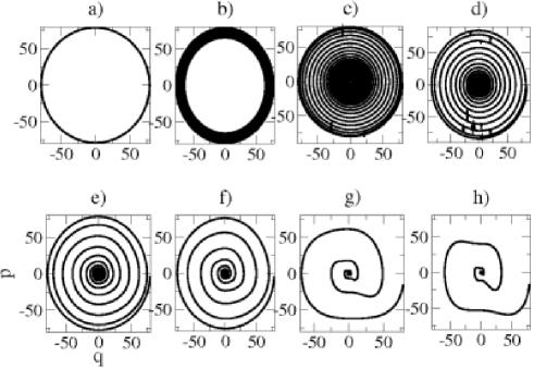
Figure 8: Phase space dynamics for $N=0,1,10,20,50,100,500,1000$ (from left to right and top to bottom).

Now we turn our attention to other types of distributions, we consider the cases for which the spectral density has the form $J(\omega)=\omega^{s}$, with $0\leq s\leq 2$ [1]. If $s=1$ the quadratic frequency distribution of the ohmic bath is recovered. For $s\leq 1$ we have the sub-ohmic bath, where lower frequencies in the chosen domain have a bigger contribution when $N$ is sufficiently large. For $s\geq 1$ we have the super-ohmic case, where higher frequencies appear more frequently.

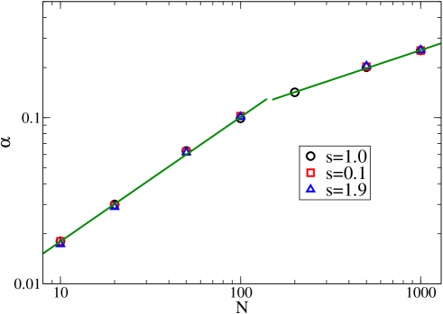
Figure 9: Exponential fits, $\alpha$, of the energy decay in the low times region for ohmic, subohmic, and superohmic baths as a function of $N$.

In Fig. 9 we plot the $\alpha$ exponents of the short time exponential decay for all the three types of baths: ohmic ($s=1.0$), sub-ohmic ($s=0.1$), and super-ohmic ($s=1.9$). One can notice very small differences from one type of the bath to another. For a better visualization we plot the results in a log-log plot. One can clearly notice two distinct behaviors, shown in the figure by continuous lines. For low values of $N$ the exponent follows a power-law with the exponent equals to $0.749$ while for high values of $N$ the best fit is another power-law function with the exponent equals to $0.362$.

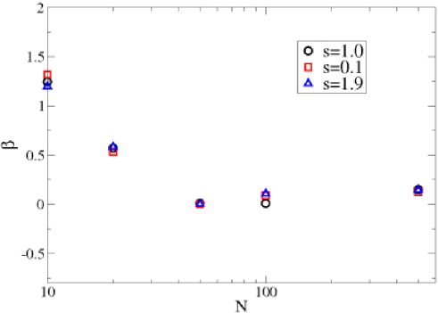
Figure 10: Power-law fits, $\beta$, of the energy decay in the long times region for ohmic, subohmic, and superohmic baths as a function of $N$.

In Figure 10 we plot the $\beta$ power-law exponents of the long times energy decay for ohmic, sub-ohmic, and super-ohmic baths. As before, there were noticed small differences in the exponents of different bath’s type. We notice a fast decrease of $\beta$ when $N$ increases. For large $N$, i.e. $N>500$, it is difficult to say that the energy decay follows a power-law function, due to the strong fluctuating behavior.

4 Morse potential

The Morse potential [39, 40, 41] is given by

$$V(r)=D_{e}[1-e^{-a(r-r_{e})}]^{2},$$ (15)

where $r$ is the distance between atoms, $r_{e}$ is the equilibrium bound distance, $D_{e}$ is the well depth, $a=\sqrt{\frac{K_{e}}{2D_{e}}}$ is the depth. $K_{e}$ is the force constant at the minimum of the well.

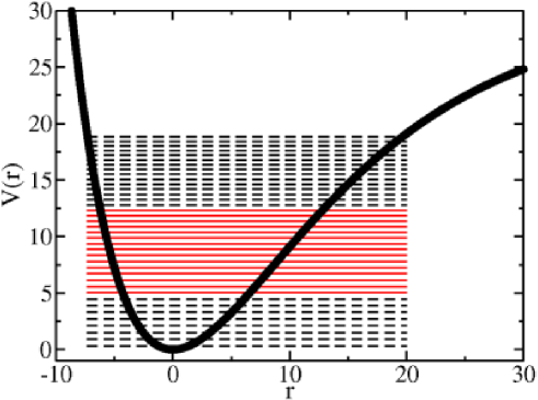
Figure 11: Morse potential for $D_{e}=30,a=0.08,r_{e}=0$. With horizontal lines are depicted the energy levels in the $r$ interval $[-7.4,20]$, with continuous lines are shown the middle energies levels used in our simulations (see the text for details).

The energy levels $\epsilon_{n}$ and the position elements $r_{nm}$ were determined by using the numerov method [42]. The results for the energy levels were comparable with the analytical form [39]:

$$\epsilon_{n}=\hbar a\sqrt{\frac{2D_{e}}{m}}(n+\frac{1}{2})-\frac{[\hbar a\sqrt{\frac{2D_{e}}{m}}(n+\frac{1}{2})]^{2}}{4D_{e}}.$$ (16)

Figure 11 shows in thick continuous line the Morse potential, given by Eq. (15), with the following values of the constants [40]: $D_{e}=30,a=0.08,r_{e}=0$. With horizontal lines are depicted all the $38$ energy levels, as calculated from the numerov method. For the simulations we used as initial condition for the coefficients $c_{n}$ a Gaussian wave packet form $\phi(r)=C\exp{-\frac{(r-16)^{2}}{\sigma^{2}}}$, where $\sigma=3$ and $C$ is the normalization constant. Thus, we will have a wave packet with the peak at the energy level $16$, placed in the middle of the energy spectrum, corresponding to the values $5.03$ to $12.32$, depicted by continuous horizontal lines in Figure 11. Here, the coefficients $c_{n}$ have the real Gaussian form defined above and they fulfill the equation $\sum_{n=9}^{23}|c_{n}|^{2}(0)=1$.

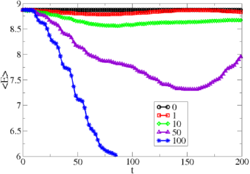
Figure 12: The energy decay, Eq. (11), for Morse potential. The number of HOs in the ohmic bath is varied: $0,1,10,50,100$.

The energy decay, Eq.(11), for a bath having $N=0,1,10,50,$ and $100$ HOs is plotted in Fig. 12. It was considered that all of them have the same mass $m=1$ and experience the same coupling strength with the system, $g_{\lambda}=g=0.001$, which is one order of magnitude smaller when compared to the HO case considered before. Here, the frequencies of the oscillators follow a quadratic distribution in the interval $[1.1,2.1]$, and for each bath, once chosen the frequencies, are kept constant. For each case, namely a bath having $N=1,10,50,$ and $100$ harmonic oscillators, we will vary only $x_{\lambda}$ and $y_{\lambda}$, which are real distributed numbers with zero mean and deviation one. For all the non-zero cases ($N\neq 0$) we took $500$ different initial conditions $(x_{\lambda},y_{\lambda})$, except the case of $N=100$, where due to the high CPU time we average over $200$ initial conditions. For the simulations we consider all the energy levels of the system, described by a wave packet of $38$ energy levels, $\epsilon_{n}$, corresponding to $38$ wavefunctions, $\phi_{n}$ (and implicitly the $c_{n}$ coefficients).

It can be easily seen that in the case of no bath $N=0$ the total energy is conserved in time. When we have the case $N=1$, in the chosen time interval, the total energy decays slowly but returns to the system at $t\sim 150$. For $N\gtrsim 10$ HOs the energy decays exponential in time, with some fluctuations, due to the stochastic average. The power-law decay observed in the HO case for later times is not seen here since the coupling to the bath is much smaller and decays occur much slower. In fact the purity (not shown) also decays much slower when compared to the HO case.

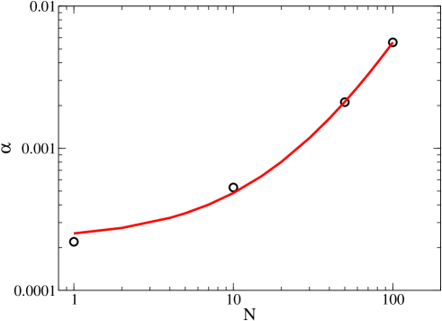
Figure 13: The exponent $\alpha$ of the energy decay as a function of $N$.

The exponential energy decays can we summarized in Fig. 13, where the values of the exponential coefficient $\alpha$ of the energy decay are plotted as a function of the number of the oscillators of the bath, $N$. For a better visualization the results are shown in a log-log plot. The situation is different than the power-law fits encountered for the harmonic potential. Here, we found that the best fit is a quadratic function given by $10^{-5}[0.0307N^{2}+2.25N+22.9]$. Thus exponential decays increase with $N$.

5 Conclusions

In this paper we use the stochastic Schrödinger equation for zero temperature to study the energy decay for a system particle, situated in a harmonic potential and in a Morse potential. The system is coupled to a bath composed of a finite number $N$ of uncoupled harmonic oscillators. For the discussions we chose, in the limit $N\to\infty$, an ohmic bath distribution, but we also study the cases of sub-ohmic and super-ohmic baths.

In the case of a harmonic potential, with coupling intensity to the bath $\gamma=0.01$, it was observed that for very small numbers $N$ the energy is exchanged back and forth into the bath. For intermediate values of $N$ around $10\leq N\leq 20$, the time average energy starts to decay, transferring partially its energy to the bath and we do not see any energy regain for the integrated times. For these values of $N$ we observed two exponential energy decays (with different exponents) for small times and a power-law decay for large times. For relatively higher values of $N$ ($\gtrsim 50$) a strong exponential decay was observed and no power-laws. Therefore, non-Markovian dynamics is expected for intermediate values of $N$ ($10\lesssim N\lesssim 20$) and a Markovian motion for larger values of $N$. The exponents for the exponential decays increase with $N$ obeying two power-laws. We analyzed also the purity of the system which gives informations about the decoherence process. Essentially decoherence occurred in all cases for short times, where exponential decays were observed for both, the energy and purity. For a system situated in a Morse potential, with coupling intensity to the bath $\gamma=0.001$, the high computational effort forced us to restrict our simulations to shorter time evolutions. Due to such small couplings, the energy and purity decays occur much slower when compared to the harmonic case and we just observed the exponential decays. Different from the harmonic case, the exponents of the exponential decay increase quadratically with $N$.

One of the main goals of this work is to show general features which occurs in systems coupled to an increasing number of bath constituents. Therefore, in addition to the above main general results, we would like to conclude with some relevant characteristics observed in the simulations but not mentioned along the text: The energy decay rate increases with increasing coupling strength between system and bath, but the time for energy regain is independent of the coupling. The energy regain time depends on the mean bath frequency and on $N$. For larger $N$ results are totally independent on the numerical frequency generator. For smaller values $1\leq N\leq 50$, the values of exponential and power-law exponents for the energy decay may change for different frequencies generator, but the overall qualitative dynamics is equivalent.

References

- [1] U. Weiss Quantum Dissipative Systems (World Scientific, Singapore, 1999)
- [2] P. Ullersma Physica 32, 27 (1966)
- [3] R. Zwanzig J. Stat. Phys. 9, 215 (1973)
- [4] E. Cortés, B. J. West, and K. Lindenberg J. Chem. Phys. 82, 2708 (1985)
- [5] H. Wang and M. Thoss J. Chem. Phys., 119, 1289 (2003)
- [6] I. Burghardt, M. Nest, and G. A. Worth J. Chem. Phys., 119, 5364 (2003)
- [7] K. H. Hughes, C. D. Christ, and I. Burghardt J. Chem. Phys., 131, 024109 (2009)
- [8] R. Martinazzo, M. Nest, P. Saalfrank, and G. F. Tantardini J. Chem. Phys., 125, 194102 (2006)
- [9] C. Meier and D. J. Tannor J. Chem. Phys., 111, 3365 (1999)
- [10] A. Ishizaki and Y. Tanimura Chem. Phys., 347, 185 (2008)
- [11] J. T. Stockburger and H. Grabert Phys. Rev. Lett., 88, 170407 (2002)
- [12] W. Koch, F. Grossmann, J. T. Stockburger, and J. Ankerhold Phys. Rev. Lett., 100, 230402 (2008)
- [13] C.-M. Goletz and F. Grossmann J. Chem. Phys., 130, 244107 (2009)
- [14] R. P. Feynman and F. L. Vernon Ann. Phys. 24, 118 (1963)
- [15] A. O. Caldeira and A. J. Leggett Physica A 121, 587 (1983)
- [16] L. Diósi and W. T. Strunz Phys. Lett. A 235, 569 (1997)
- [17] W. T. Strunz, L. Diósi, N. Gisin, and T. Yu Phys. Rev. Lett. 83, 4909 (1999)
- [18] J. Rosa and M. W. Beims Phys. Rev. E 78, 031126 (2008)
- [19] C. Manchein, J. Rosa, and M. W. Beims Physica D 238, 1688 (2009)
- [20] M. Sarovar, A. Ishizaki, G. R. Fleming, and K. B. Whaley Nature Phys. 6, 462 (2010)
- [21] G. D. Scholes Nature Phys. 6, 402 (2010)
- [22] S. Bay, P. Lambropoulos, and K. Molmer Phys. Rev. Lett. 76, 161 (1996)
- [23] J. J. Hope Phys. Rev. A 55, R2531 (1997)
- [24] S. John and T. Quang Phys. Rev. Lett. 74, 3419 (1994)
- [25] N. Vats and S. John Phys. Rev. A 58, 4168 (1998)
- [26] G. M. Moy, J. J. Hope, and C. M. Savage Phys. Rev. A 59, 667 (1999)
- [27] Ph. Blanchard et. al. (Eds.), Decoherence: Theoretical, Experimental, and Conceptual Problems, Lecture Notes in Physics; 538, (Springer, Heidelberg), (2000)
- [28] W. H. Zurek Physics Today, October 1991, 36 (1991)
- [29] D. Giulini, E. Joos, C. Kiefer, J. Kupsch, I. O. Stamatescu, and H. D. Zeh Decoherence and the Appearance of the Classical World (Springer, Berlin), (1996)
- [30] V. Wong and M. Gruebele Chem. Phys. 284, 29 (2002)
- [31] W. Koch, F. Grossmann, J.Stockburger, and J. Ankerhold Chem. Phys. 370, 34 (2010)
- [32] R. M. Angelo Phys. Rev. A 76, 052111 (2007).
- [33] Y. Elran and P. Brumer J. Chem. Phys. 121, 2673 (2004)
- [34] W. T. Strunz Phys. Lett. A 224, 25 (1996)
- [35] T. Yu, L. Diósi, N. Gisin, and W. T. Strunz Phys. Rev. A 60, 91 (1999)
- [36] L. Diósi Quantum Semiclassic. Opt. 8, 309 (1996)
- [37] A. M. Walsh and R. D. Coalson Chem. Phys. Lett. 198, 293 (1992)
- [38] W. H. Press, S. A. Teukolsky, W. T. Vetterling, B. P. Flannery Numerical Recipes in Fortran, (Cambridge University Press, USA, 1992)
- [39] L. D. Landau and E. M. Lifschitz Quantenmechanik, (Akademie - Verlag, Berlin, 1986)
- [40] P.-N. Roy and T. Carrington Jr. Chem. Phys. Lett. 257, 98 (1996)
- [41] P. M. Morse Phys. Rev. 34, 57 (1929)
- [42] V. Fack and G. Vanden Berghe J. Phys. A: Math. Gen. 20, 4153 (1987)