Adding particle collisions to the formation of
asteroids and Kuiper
belt objects via streaming instabilities
Modelling the formation of super-km-sized planetesimals by gravitational collapse of regions overdense in small particles requires numerical algorithms capable of handling simultaneously hydrodynamics, particle dynamics and particle collisions. While the initial phases of radial contraction are dictated by drag forces and gravity, particle collisions become gradually more significant as filaments contract beyond Roche density. Here we present a new numerical algorithm for treating momentum and energy exchange in collisions between numerical superparticles representing a high number of physical particles. We adopt a Monte Carlo approach where superparticle pairs in a grid cell collide statistically on the physical collision time-scale. Collisions occur by enlarging particles until they touch and solving for the collision outcome, accounting for energy dissipation in inelastic collisions. We demonstrate that superparticle collisions can be consistently implemented at a modest computational cost. In protoplanetary disc turbulence driven by the streaming instability, we argue that the relative Keplerian shear velocity should be subtracted during the collision calculation. If it is not subtracted, density inhomogeneities are too rapidly diffused away, as bloated particles exaggerate collision speeds. Local particle densities reach several thousand times the mid-plane gas density. We find efficient formation of gravitationally bound clumps, with a range of masses corresponding to contracted radii from 100 to 400 km when applied to the asteroid belt and 150 to 730 km when applied to the Kuiper belt, extrapolated using a constant self-gravity parameter. The smaller planetesimals are not observed at low resolution, but the masses of the largest planetesimals are relatively independent of resolution and treatment of collisions.
Key Words.:
hydrodynamics – methods: numerical – minor planets, asteroids: general – planets and satellites: formation – protoplanetary disks – turbulenceA. Johansen ()
1 Introduction
The formation of super-km-sized planetesimals is an important step towards terrestrial planets and the solid cores of gas and ice giants (e.g. Safronov, 1969; Goldreich et al., 2004; Chiang & Youdin, 2010). The asteroid and Kuiper belts of the solar system, as well as the extrasolar debris discs, are believed to be left-over populations of planetesimals that did not grow to planets. Comparing models and simulations of planetesimal formation to observations of such planetesimal belts constrains our theoretical picture of the planetesimal formation stage, and at the same time it gives insight into the physical processes that shaped the architectures of these systems (Morbidelli et al., 2009; Weidenschilling, 2010; Nesvorný et al., 2010; Sheppard & Trujillo, 2010; Krivov, 2010; Kenyon & Bromley, 2010).
Planetesimal formation takes place in a complex environment of turbulent gas interacting via drag forces with particles of many sizes. The streaming instability thrives in the systematic relative motion of gas and particles and leads to spontaneous clumping of particles (Youdin & Goodman, 2005; Johansen & Youdin, 2007; Bai & Stone, 2010b), seeding a gravitational collapse into bound clumps (Johansen et al., 2009) and further to solid planetesimals (Nesvorný et al., 2010). While the latest years have seen major progress in numerical modelling of drag force interaction between particles and gas (Youdin & Johansen, 2007; Balsara et al., 2009; Miniati, 2010; Bai & Stone, 2010a) as well as the self-gravity of the particle layer (Johansen et al., 2007; Rein et al., 2010), good algorithms for treating simultaneously hydrodynamics, gravitational dynamics and particle collisions are still missing.
There are two main approaches in astrophysics to treating particle collisions in numerical simulations. Modelling a set of physical particles with collision tracking allows simulation of particle aggregation in close concordance with the nature of real physical collisions. This method has successfully been applied to model the particle rings of Saturn (Wisdom & Tremaine, 1988; Salo, 1991; Karjalainen & Salo, 2004) and to model collisions between individual dust grains and aggregates (Dominik & Nübold, 2002). The drawback of the physical-particle approach is that the size of the system is limited by the number of numerical particles that can be afforded in the simulation. The formation of a Ceres-mass planetesimal from 10-cm-sized rocks would e.g. require tracking of particles, orders of magnitude beyond what current computational resources allow.
Algorithms involving inflated particles group collections of physical particles into much larger numerical particles under conservation of total mass and mean free path . Decreasing the particle number to a number that can be handled in a computer simulation, while maintaining by artificially increasing the collisional cross section , yields the correct collision frequency in systems that are much larger than what can be resolved with the physical particle approach. The inflated particle approach was used recently by Lithwick & Chiang (2007), Michikoshi et al. (2007), Nesvorný et al. (2010), and Rein et al. (2010), with different methods for tracking the actual collision, but the concept of bloated particles has deeper roots (e.g. Kokubo & Ida, 1996).
In this paper we put forward a new algorithm to model collisions between numerical superparticles. Superparticles are designed to represent swarms of physical particles. The aerodynamical properties of the superparticle (e.g. the friction time) is still that of a single physical particle. Superparticles are widely used to model the solid particle component in computer simulations of coupled gas and particle motion in protoplanetary discs (Johansen & Youdin, 2007; Bai & Stone, 2010b). Since superparticles can be considered to represent swarms of smaller particles, direct collision tracking is not possible. Johansen et al. (2007) modelled superparticle collisions by damping the random motion of particles inside a grid cell on the collisional time-scale. They showed that inelastic collisions, where part of the kinetic energy is converted to heat and deformation during the collisions, is beneficial for the gravitational collapse and allows the formation of planetesimals in protoplanetary discs of lower mass, compared to simulations without damping. However, the simplified collision scheme of Johansen et al. (2007) is insufficient in capturing the pairwise momentum exchange and energy dissipation.
We develop here a statistical approach to model the full momentum exchange and energy dissipation in collisions between superparticles. The Monte Carlo scheme is inspired by the collision algorithms presented by Lithwick & Chiang (2007) and Zsom & Dullemond (2008). The essence of our algorithm is to determine the collision time-scale between all superparticle pairs within a grid cell. Two superparticles collide as if they were physical particles touching each other, if a random number chosen uniformly between zero and one is smaller than the ratio of the simulation time-step to the collision time-scale.
Collisions can be followed together with hydrodynamics at a moderate computational cost depending only on the number of particles per grid cell. We compare the statistical properties of the particle density in 3-D hydrodynamical simulations with and without collisions. Including the self-gravity of the particles, we find formation of bound clumps, with masses comparable to that of the 500-km-radius dwarf planet Ceres when applied to the asteroid belt, relatively independently of numerical resolution and treatment of collisions. The scale-free nature of our simulations allows application of the results to the Kuiper belt as well, with contracted planetesimal radii approximately 80% higher than in the asteroid belt.
The paper is organised as follows. In Sect. 2 we describe the new superparticle collision algorithm. The algorithm is tested against known test problems and conservation properties of the shearing box in Sect. 3. In Sect. 4 we analyse statistical properties of the particle density achieved in simulations of gas and particle turbulence driven by the streaming instability. We continue to include self-gravity in the simulations and analyse the planetesimal masses obtained under various assumptions about collisions in Sect. 5. We summarise and discuss our results in Sect. 6. The appendices A–C contain further descriptions of the collision algorithm.
2 Superparticle collision algorithm
We will use the notation that a superparticle represents a swarm of physical particles with number density and volume . Since we are interested in coupling superparticle collisions to grid hydrodynamics, the volume is taken to be that of a grid cell, . The physical particles in the swarm have individual mass, physical radius, material density, and collisional cross section , , and . We assume that all swarms are similar, both in internal particle number and in the physical mass of the constituent particles.
To track a collision we calculate the mean free path for a test particle interacting with the swarm of particles represented by a single superparticle,
| (1) |
Superparticles in the same grid cell are considered as potential colliders. For each collision pair the collision time-scale is calculated from
| (2) |
where is the relative speed between particles and . The simulation time-step , set by hydrodynamics and drag forces, is then used to calculate the probability that those two particles collide in this time-step,
| (3) |
Two colliding swarms have their velocity vectors changed instantaneously. The collision outcome is found by considering two virtual spherical particles whose surfaces touch, with particle centres at the locations of the superparticles, and solving for momentum conservation and inelastic energy dissipation (or energy conservation, in case of elastic collisions). We define the velocity vectors relative to the mean velocity field ,
| (4) | |||||
| (5) |
Here and are the velocity vectors of the two particles111We show in Sect. 3.2.1 that the Keplerian shear should be subtracted from the velocity vectors when determining both the collision time-scale and the collision outcome, in the limit of particles that are much smaller than a grid cell.. The normal vector connecting the centres of the particles at the time of collision is calculated as
| (6) |
The parallel vector is perpendicular to in the same plane as the relative velocity vector. The relative velocity vectors are now decomposed on the two directions
| (7) | |||||
| (8) |
with and . In the collision we maintain , while we reflect according to
| (9) |
Here is the coefficient of restitution, parameterising the degree of energy dissipation during the collision. Inelastic collisions can play an important role in dissipating kinetic energy and facilitating the gravitational collapse phase. In general the coefficient of restitution depends on material parameters, impact speed and ambient temperature. Water ice particles have been measured to have a high coefficient of restitution for impact speeds below m/s (quasi-elastic regime of Higa et al., 1996). Above this critical speed the measured coefficient of restitution rapidly drops towards zero. More recent microgravity and drop tower experiments find a coefficient of restitution between 0.06 and 0.84 in low-velocity collisions between 1.5-cm-sized icy pebbles (Heißelmann et al., 2010). In this paper we consider for the sake of simplicity the coefficient of restitution to be a constant that is independent of the relative speed.
The collision time-scale has a simple relation to the friction time-scale when particles are small and drag forces are in the Epstein regime. We show in Appendix A how the collision time-scale can be easily calculated from the friction time-scale, useful e.g. for simulations of gas and particles in protoplanetary discs.
Consider now a grid cell containing superparticles. For particle the collision probability for a representative particle222Zsom & Dullemond (2008) define a representative particle from a swarm as a test particle (a random particle from the swarm) used to probe the collision time-scale with another swarm. from superparticle to collide with the particle swarms to is calculated. The collision occurs if a random number, drawn for each collision partner, is smaller than from Eq. (3). The collision instantaneously changes the velocity vectors of both particles and . This way the correct collision frequency is obtained for both particles, even though the algorithm only considers the possible collision with , but not with . In Appendix B we describe how to consistently limit the number of collision partners, and thus save computation time, in grid cells which contain many ( 100) particles.
There are several advantages to using such a probabilistic swarm approach to particle collisions. We mention here a few: (i) it is fast because we do not have to track when particles touch or overlap within the grid cells, (ii) it allows us to freely choose the relative speed that enters the collision frequency, useful e.g. for subtracting off the Keplerian shear (see Sect. 3.2.1), and (iii) the algorithm is easily generalisable to also include a probabilistic approach to particle coagulation and shattering.
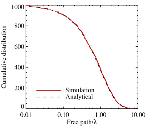
In Fig. 1 we show the collision path length of test particles injected into a medium with 10 superparticles per grid cell and a mean free path of . Collisions are tracked through the Monte Carlo method described above. The collision algorithm makes some particles collide after a short flight path and others after a longer. The distribution plotted in Fig. 1 follows closely the expectation . The Monte Carlo approach to collisions is very similar to the physical particle approach in the distribution of free flight paths.
The main technical difference between using inflated particles (see introduction) and our newly developed collision algorithm for superparticles is that inflated particles always collide when they overlap physically (the particle size can be associated with the grid cell size), while superparticles sharing the same grid cell collide with a certain probability which guarantees that collisions occur on the average after a collisional time-scale. Another difference is that superparticles which do not approach must still be allowed to collide, as otherwise the mean free path will be too long. Non-approaching particles are collided by flipping the relative velocity vector before collision and reflipping afterwards. The main issue with approaching collisions is that collisions occur in fixed grid cells which are not centred on the superparticle in question, and thus a superparticle at the edge of a grid cell will have too few collision partners if only approaching collisions are allowed. We show in Appendix C how the superparticle approach transforms smoothly to the inflated particle approach when the number of superparticles is reduced.
The Monte Carlo collision scheme presented here could equally well be formulated in terms of inflated particles, by constructing inflated particles smaller than a grid cell. Solving statistically for the collision outcome of these “sub-grid” particles is mathematically equivalent to the interpretation, chosen for this paper, of the numerical particles as swarms.
3 Validation of algorithm
We have implemented the Monte Carlo superparticle collision scheme described in Sect. 2 into the open source code Pencil Code333The code, including the developments described in this paper, can be freely downloaded at http://code.google.com/p/pencil-code/.. The Pencil Code evolves gas on a fixed grid and has fully parallelised modules for an additional solid component represented by superparticles (Johansen et al., 2007; Youdin & Johansen, 2007). We first validate the collision algorithm in the limit of inflated particles (i.e. where two particles occupying the same grid cell always collide and only approaching collisions are considered), to compare our results directly to those of Lithwick & Chiang (2007). The 2-D algorithm of Lithwick & Chiang (2007) has a probabilistic approach to determine whether two particles are in the same vertical zone when they overlap in the plane. Their algorithm can thus be seen as a hybrid of the inflated particle approach and a Monte Carlo scheme.
We set up a test problem similar to the one presented in Lithwick & Chiang (2007). We define a 2-D simulation box covering the spatial interval with grid cells in both the and direction. particles are placed randomly in a ring of full width centred at the radial distance . A central gravity source, of strength , is placed in the centre of the coordinate frame.
We integrate the particle orbits, including collisions, for revolutions of the ring centre. In order to compare directly with Lithwick & Chiang (2007) we use their 2-D approximation. The particle number density can be approximated as , where is the column (number) density and is the scale height of the particle disc. The random particle motion can be written as . This yields a collision time
| (10) |
where is the vertical optical depth of the disc and is the orbital time-scale. While the collision time-scale in general depends on the random particle motion, this dependence vanishes in the 2-D Keplerian disc approximation – faster random motion cancels with increased particle scale-height in the collision time expression.
Requiring that orbits are maintained for orbital time-scales, we set the time-step of the Pencil Code to , covering each orbit by around 600 time-steps. This proved necessary because the third order time integration scheme of the Pencil Code is not constructed to conserve orbital angular momentum and energy. Using the highly optimized orbital dynamics code SWIFT, Lithwick & Chiang (2007) solve the same problem with slightly less than five time-steps per orbit.
In Fig. 2 we show the eccentricity evolution of the particle ring. For a coefficient of restitution of the particles relax to an equilibrium eccentricity of around , comparable to . A higher coefficient of restitution of leads instead to catastrophic heating of the disc (Goldreich & Tremaine, 1978), with an eccentricity that evolves linearly with time. The results presented in Fig. 2 show that the superparticle collision algorithm is in excellent agreement with Lithwick & Chiang (2007) in the limit of inflated particles.

3.1 Density evolution
The width of a particle ring increases due to collisional viscosity. Since the collision time-scale scales inversely with particle density, the collisional evolution slows down with time. An analytical solution to the diffusion problem was found by Petit & Henon (1987). In the notation of Lithwick & Chiang (2007) the width of an initially narrow ring increases according to
| (11) |
Here is a dimensionless factor that depends on the coefficient of restitution , is the grid spacing, is the mean radial coordinate of the particles, is the particle number and the time.
We follow Lithwick & Chiang (2007) and define an initially very narrow ring of radial extent . The units follow from our choice of . The evolution of the radial width is shown in Fig. 3 over orbits. We overplot the analytical solution for , similar to the fit in Lithwick & Chiang (2007), and find excellent agreement.

3.2 Superparticle collisions in the local frame
Hill’s equations describe motion relative to a frame that corotates with the Keplerian frequency at an arbitrary distance from the central gravity source. The coordinate axes are defined such that points radially outwards and points along the flow of the disc. The 2-D equations of motion of particles are
| (12) | |||||
| (13) |
Particle positions are evolved through . The boundary conditions are periodic in the azimuthal direction. Particles passing over the inner (outer) radial boundary get the velocity subtracted (added) to their azimuthal velocity. We also refer to the frame as the shearing box. We consider a box size of covered by grid cells and particles.
The conserved energy (Jacobi constant) is
| (14) |
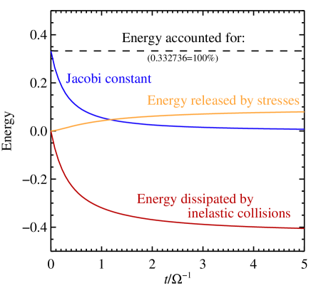
Elastic collisions re-orient the particles without changing energy, and thus convert circular orbits into eccentric ones while conserving energy. Ignoring gas, which damps the velocity relative to the gas and hence the eccentricity, elastic collisions conserve the Jacobi energy. Fig. 4 shows the energy of particles versus time in local frame simulation with inelastic collisions. Particles are initialised with random position and velocity vectors (). The mean-free-path is , giving an initial collision time-scale of . The coefficient of restitution is . The Jacobi constant falls with time due to the energy dissipated by inelastic collisions. At the same time particles passing over the radial boundaries release energy from the Keplerian shear through their mean Reynolds stress (the code tracks and outputs that energy release for each particle passing the radial boundary). All energy in the system is accounted for in these three reservoirs.
3.2.1 Shear during collision
Particle collisions in the shearing box release energy from the Keplerian shear into random motion, leading in the absence of drag forces either to catastrophic heating () or to an equilibrium with energy dissipation in inelastic collisions ( where is the particle radius). Discounting the former option, the result of the latter can be artificially exaggerated by the numerical scheme because we identify the collision between two superparticle swarms with the collision between two members of the swarms located at the respective swarm centres. In reality collisions would occur between neighbouring particles separated by less than their physical diameter. The naive numerical algorithm would make the system settle for an equilibrium where , where is the grid spacing and also the typical distance between superparticle centres. This rms speed greatly exceeds the desired . In other words, the naive collision algorithm will input artificial heating.
| Run | Collisions | |||||||
|---|---|---|---|---|---|---|---|---|
| SI64_nocoll | – | – | 100 | – | ||||
| SI64_e1.0 | KS | 100 | – | |||||
| SI64_e0.3 | KS | 100 | – | |||||
| SI64_e0.3_NS | NS | 100 | 52 | |||||
| SI128_nocoll | – | – | 50 | – | ||||
| SI128_e1.0 | KS | 50 | – | |||||
| SI128_e0.3 | KS | 50 | – | |||||
| SI128_e0.3_NS | NS | 50 | 19 |
Col. (1): Name of simulation. Col. (2): Box size in scale heights. Col. (3): Resolution. Col. (4): Number of particles. Col. (5): Friction time. Col. (6): Collision type. Col. (7): Coefficient of restitution. Col. (8): Simulation time in orbits. Col. (9): Time of starting self-gravity.
Collisions between particles of radius can be modelled by subtracting the Keplerian shear part from the relative speed both for determining the collision time-scale and for determining the outcome of the collision. Decomposing the azimuthal velocity field as , where is the Keplerian shear velocity and is the peculiar velocity, we can calculate both the collision time-scale and outcome in terms of (together with and ). Lyra et al. (2009) applied a similar trick to subtract off the entire (Keplerian plus peculiar) gas velocity from the particle velocity. However, two particles moving at the same velocity as the local gas do not necessarily avoid collisions, even if the gas is incompressible, since the particle motion is not completely coupled to the gas. Therefore we choose in this paper to subtract off only the Keplerian orbital speed from the particle velocity. The dynamical equations of the Pencil Code are already formulated relative to the Keplerian shear, so subtracting off the shear is natural to the governing system of equations.
Collisions relative to the Keplerian shear conserve both the total momentum and the momentum relative to the Keplerian shear, but the energy in elastic collisions is only conserved relative to the Keplerian shear. To see this, consider the kinetic energy of two particles,
| (15) |
Here is the mass of a superparticle, assumed to be the same for both colliders. An elastic collision solved in terms of (, , , ) conserves both the sum of the squares of those velocity components, as well as the squares of and (the latter is true since the position is not changed by the collision). The difference in energy before and after the collision is therefore
| (16) |
This result holds also in 3-D. The energy difference is generally not zero, even though by momentum conservation, since the offset is not the same for the two particles. The non-conservation is nevertheless small: the azimuthal velocity change in the collision is uncorrelated with the Keplerian shear velocity, so . The particle integrator’s slight non-conservation of Keplerian orbits is not a serious limitation in simulations where the dynamics is driven by hydrodynamical instabilities and drag forces. The correct relative Keplerian shear based on the physical size of the particles can in principle be added artificially, to obtain the correct energy release from the shear, but this is negligible for 1–10 cm particles considered in this paper.
The total angular momentum of two colliding particles,
| (17) |
is conserved in the collisions, both with and without Keplerian shear in the collision, as long as the force during the collision acts along the line connecting the two particles. This is the case both with and without Keplerian shear. For equal-mass particles we can write the change in the velocity as , giving
| (18) |
The above arguments for energy and angular momentum conservation are generalisible to distinct particle masses as well. However, while the Monte Carlo collision scheme in itself is fully consistent with distinct particle masses, correct energy equipartition among particle sizes can not be obtained with equal-mass superparticles (see discussion in Appendix A.1).
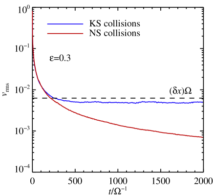
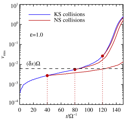
In the following we use the abbreviations KS for collisions that include Keplerian shear and NS for collisions where the Keplerian shear is subtracted off when determining the collision time-scale and outcome. Fig. 5 shows the evolution of the particle rms speed in a shearing box simulation. The top panel shows the decay of initially random particle motion by inelastic () collisions for KS collisions and for NS collisions. KS collisions decay towards , the random motion released by the Keplerian shear in a single collision. NS collisions on the other hand continue to decay towards zero. In the bottom panel of Fig. 5 we start with zero random motion and observe how elastic () KS collisions heat up the system. Rerunning the simulation with elastic NS collisions from various starting times of the KS simulation shows clearly that the evolution of the system is very similar as long as the particle rms speed is larger than . In actual simulations with gas and hydrodynamical instabilities driving particle dynamics with characteristic motion much faster than , one can subtract off the Keplerian shear term when determining the time-scale and outcome of collisions and still model the correct system, without any spurious energy released by bloated particles.
4 Particle collisions and the streaming instability
Armed with a collision algorithm for superparticles, we are now ready to explore the effect of particle collisions on particle concentration by streaming instabilities and planetesimal formation by self-gravity. The streaming instability feeds off the relative (streaming) motion of gas and particles in protoplanetary discs and has a characteristic length scale comparable to the sub-Keplerian length (Youdin & Goodman, 2005). Here is the radial pressure gradient parameter of Nakagawa et al. (1986) and is the distance to the central star. Johansen et al. (2009) and Bai & Stone (2010b) demonstrated that the streaming instability leads to strong particle clumping when the heavy element abundance of the disc is above a threshold value of for particle sizes (and moderate radial drift, see Bai & Stone, 2010c). Clumping proceeds as initially very low amplitude particle overdensities accelerate the gas towards the Keplerian speed, hence reducing the local head-wind, which in turn slows the radial drift of the particles. Drifting particles pile up where the head-wind is slower, causing exponential growth of the particle density as the particles continue to increase their drag force influence on the gas. Johansen et al. (2009) found that overdense regions contract when including particle self-gravity and that eventually a number of gravitationally bound clumps form. These models nevertheless did not include any particle collisions.
We perform 3-D simulations where the gas is modelled on a fixed grid and solid particles with superparticles. We solve the standard shearing box equations for gas and particles (same as in Johansen & Youdin, 2007, but with additional vertical gravity). The frame rotates at the Keplerian frequency at a fixed orbital distance from the star. The coordinate axes are oriented such that points radially outwards, points along the rotation direction of the disc, while points perpendicular to the disc along . The gas is subjected to a radial pressure gradient which reduces its orbital speed by the positive amount . Particles do not feel this radial pressure gradient, and the resulting relative motion between particles and gas drives the streaming instability (Goodman & Pindor, 2000; Youdin & Goodman, 2005). We consider a cubic box with side lengths , where is the gas scale height, to capture the fastest growing modes of the streaming instability of marginally coupled particles, . This is also the characteristic scale of Kelvin-Helmholtz instabilities, thriving in the vertical shear in the gas and particle velocity (Youdin & Shu, 2002; Lee et al., 2010), although Bai & Stone (2010b) demonstrated that the streaming instability is dominant over Kelvin-Helmholtz instabilities in setting the dynamics of particle layers with .
The friction time of the particles is fixed at in all simulations, corresponding to approximately 20-cm rocks around the location of the asteroid belt at 3 AU, and to 6-mm pebbles at 30 AU (Weidenschilling, 1977). The particle column density is set to 2% of the total gas column density, the latter including the gas beyond the vertical boundaries of the box. For our choice of strong particle clumping can only be obtained at such super-solar metallicity444The threshold for clumping can be estimated analytically to be (Youdin & Shu, 2002). Bai & Stone (2010c) and Johansen et al. (2007) confirmed numerically that the threshold for particle clumping by the streaming instability shifts towards higher (lower) metallicity as the sub-Keplerian speed difference is increased (decreased).. The average dust-to-gas ratio in a box of is when . We set sound speed , Keplerian frequency and mid-plane gas density to unity, so these form the natural units of the simulations.
We compare results obtained without and with particle collisions. Simulations with particle collisions are run in three variations: either with elastic collisions (), with inelastic collisions () or with inelastic collisions where Keplerian shear is subtracted off when determining the time-scale and outcome of collisions. Simulation parameters are given Table 1. Each particle swarm contains a mass per volume of for the considered particle number at both and .
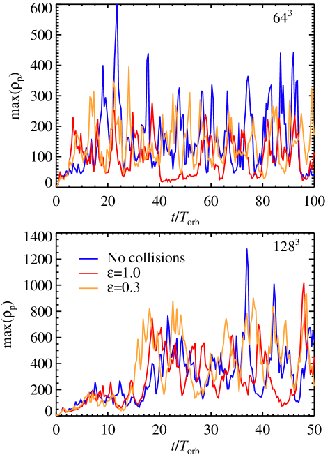
4.1 Maximum particle density
We monitor the maximum particle density regularly in the simulations. In Fig. 6 we show the maximum particle density versus time in simulations with grid cells and grid cells, respectively. Simulations without collisions generally achieve higher particle density – up to 600 times the gas density at and 1200 times the gas density at . Elastic collisions and inelastic collisions with give very high particle densities too, but the peaks have an approximately 50% lower value than in simulations without collisions. Elastic collisions achieve a somewhat lower maximum density than inelastic collisions. The kinetic energy dissipation in inelastic collisions reduces the random motion of the particles and allows higher particle contraction.
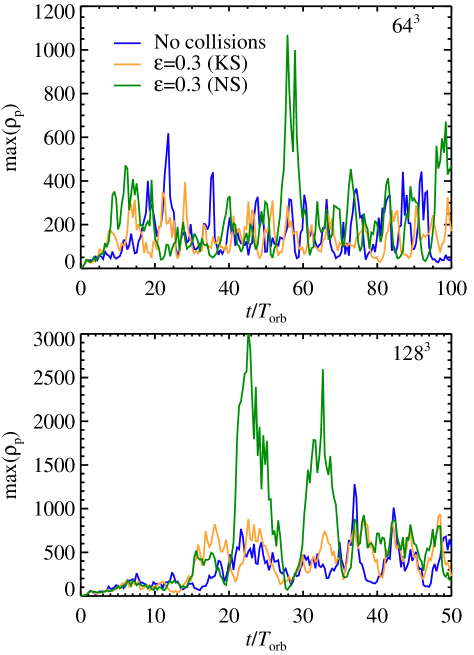
The inclusion of Keplerian shear during the collision can lead to unphysical results, since the shear term is exaggerated by enlarging particles to the size of a grid cell. The exaggerated kinetic energy input will in turn suppress concentration peaks, in agreement with what is seen in Fig. 6. In Fig. 7 we show the maximum density in simulations with inelastic KS and NS collisions respectively (and the results without collisions for comparison). Simulations with NS collisions display a three times higher maximum density than simulations with KS collisions. The maximum density is even a factor 2-3 times higher than in simulations without collisions. This way collisions actually promote particle concentration.
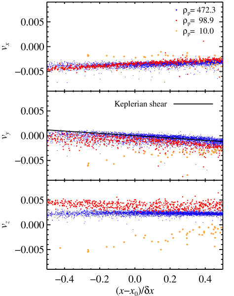
In Fig. 8 we analyse the particle motion within three grid cells of the run SI_128_e0.3. We choose the grid cell with the maximum particle density in the box and two grid cells with a particle density close to 100 and 10 times the gas density, respectively. The particle velocity shows both systematic trends and random motion within the cells. The random motion is slower in the cells of higher density. The Keplerian shear is clearly visible in the -velocity of particles in the two densest grid cells. Thus the hydrodynamical simulations are prone to spurious heating, as explained above. Subtracting off the Keplerian shear term when determining the time-scale and outcome of collisions avoids this problem. Fig. 8 also shows a systematic trend in the radial particle velocity. Radial convergence and divergence in the particle velocity are expected when particles concentrate in radial bands and when the concentrations dissolve again. We do not attempt to correct for this systematic velocity within grid cells, but note that systematic trends from smooth gradients will decrease with increasing resolution.
4.2 Particle concentration versus scale
Overdense particle sheets contract radially under the action of self-gravity and drag forces (Youdin, 2011; Michikoshi et al., 2010; Shariff & Cuzzi, 2011). A full non-axisymmetric collapse is initiated when the particle density crosses the Roche density
| (19) |
The mass of the planetesimal will be characterized by the scale over which the Roche density is achieved. To quantify the scale-dependence of the particle concentrations, we measure the maximum particle density over cubic regions of side length grid cells, increasing from 1 to . We ensure that all concentrations centres are probed by stepping the measurement region through the entire grid. Measurement regions crossing the boundaries are handled by expanding the particle density field with its periodic counterpart in all directions (glueing together copies which are identical except for a shift due to Keplerian shear).
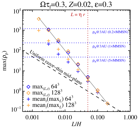
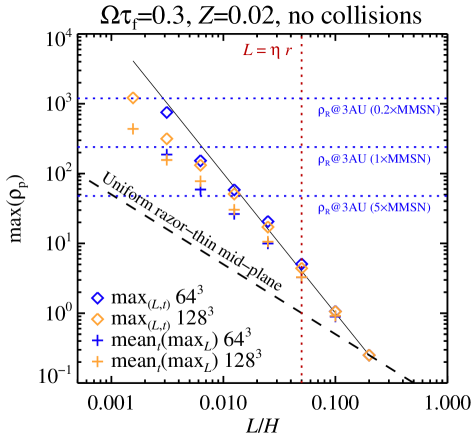
For snapshots saved once per orbit from to we calculate the maximum particle density as a function of scale. The results are shown in Fig. 9 for simulations with NS collisions (SI64_e0.3_NS and SI128_e0.3_NS) in the top panel and simulations with no collisions (SI64_nocoll and SI128_nocoll) in the bottom panel. We extend the measurements of SI64_e0.3_NS to to catch a major concentration event (see top panel of Fig. 7). We indicate in Fig. 9 both the maximum density over all times and the mean of the time-dependent maximum density. The maximum scale-dependent density in NS simulations is very similar at and at . This quantity is nevertheless very sensitive to the low-number statistics of the concentration events. A more robust measure is the mean of the maximum density. This measure increases somewhat from to . It is also evident from Fig. 7 that major concentration events have a higher temporal filling factor at . Whether this is intrinsic to the streaming instability dynamics or just an effect of running simulations for too short time is not possible to discern.
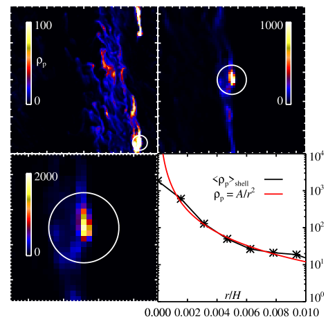
The apparent linear decrease of logarithmic density with logarithmic scale implies as a good model for the scale-dependence of the maximum density. Two limits can immediately be put on . The lowest value would stem from a razor-thin particle mid-plane layer of uniform density, with , giving and thus . Concentration of all particles in a single point would yield the upper limit of . We overplot in Fig. 9 with a thin black line the power law , fitted to match the mean density of the box at . The power law follows the data extremely well. This implies that , i.e. that the particles primarily concentrate either in 1-D filaments or in spherically symmetric clouds of density , known in star formation as the singular isothermal sphere solution (e.g. Shu, 1977). In Fig. 10 we show the particle density around the densest grid point in SI128_e0.3_NS at . The overdense structure appears elongated along the -direction with the density falling rapidly towards all directions (although slower along ).
Simulations without collisions (bottom panel of Fig. 9) show similar trends as the simulations with NS collisions, but there is a marked decrease in the maximum density over the smallest shared scale between and . Nevertheless the mean of the maximum density agrees between the two resolutions.
The convergence in scale-dependent maximum density shows that the dynamics of the streaming instability concentration events is well-resolved and independent of dissipation scale and viscosity. This is in contrast to turbulent concentration in driven isotropic turbulence which, for a given particle size, appears on length scales that are fixed relative to the Kolmogorov (viscous) scale (Hogan & Cuzzi, 2007; Pan et al., 2011). In contrast the streaming instability is fixed relative to the sub-Keplerian scale . At , probed only at , the maximum density in simulations with NS collisions reaches more than three thousand times the gas density. Higher resolution simulations will be needed to test if the particle density continues to follow the trend, or eventually finds a smallest scale. The 2-D streaming instability simulations of Bai & Stone (2010a) converged in density statistics at between and grid cells. Reaching those resolutions in 3-D is very computationally demanding, but should be an important priority for the future.
5 Planetesimal formation
The gravitational potential field of the particles is found by mapping the particle density on the grid, using a second order spline interpolation scheme, and solving the Poisson equation using a fast Fourier transform method (Johansen et al., 2007). The gravitational acceleration is interpolated back to the particle positions using second order spline interpolation. The strength of the gravity is defined by the non-dimensional parameter
| (20) |
which is related to the thin-disc self-gravity parameter through (Safronov, 1960; Toomre, 1964). The solar nebula of Hayashi (1981) has at 3 AU from the sun, the parameter depending weakly on the distance. We use as a reference choice in the simulations, but experiment with down to 0.02.
The total particle mass in the box is
| (21) |
where the mass unit depends on the temperature and location in the disc [] and the strength of the self-gravity []. While the expression in Eq. (21) does not depend on , in units where , the physical mass unit does. In a nebula with the scale-height given by Hayashi (1981), we have at with a mass unit of and .
We activate particle self-gravity in simulations of the streaming instability with inelastic NS collisions, at times when there is little particle concentration, to catch the simultaneous action of streaming instability and self-gravity during the next concentration event. In SI64_e0.3_NS we thus start self-gravity at , while in SI128_e0.3_NS we start self-gravity at (see Fig. 7). We then evolve the simulation for another 5 orbits, either ignoring collisions or applying the usual variation of collision types (elastic, inelastic KS, inelastic NS).
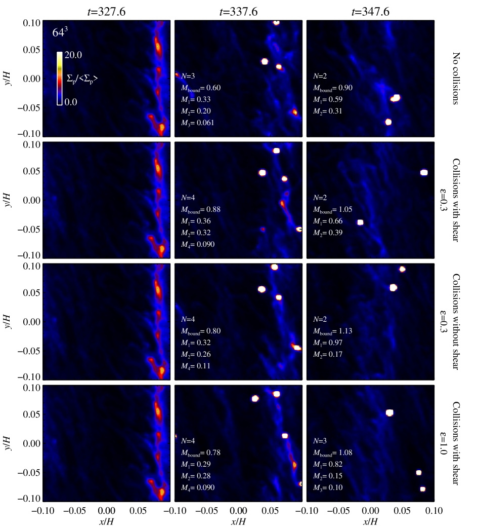
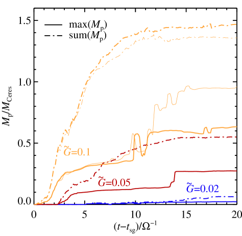
Results of simulations are shown in Fig. 11. Between 3 and 4 clumps555The algorithm for identifying bound clumps is based on 2-D column density snapshots and is described in detail in Johansen et al. (2011). initially condense out of the dominantly axisymmetric filament forming by the streaming instability. These clumps have masses between a tenth and a third of the dwarf planet Ceres – corresponding to contracted radii between 220 and 330 km, assuming an internal density of 2 g/cm3. All the clumps form in a single planetesimal-formation event shortly after the onset of self-gravity. The clumps continue to grow mainly by accreting particles from the turbulent flow, but no new gravitationally bound clumps form. Clumps eventually collide and merge in all simulations. Such clump merging is likely an unphysical effect driven by the large sizes of the planetesimals. The self-gravity solver does not allow gravitational structures to become smaller than a grid cell, and that leads to artificially large collisional cross sections. A more probable outcome of the real physical system is gravitational scattering and/or formation of binaries (Nesvorný et al., 2010).
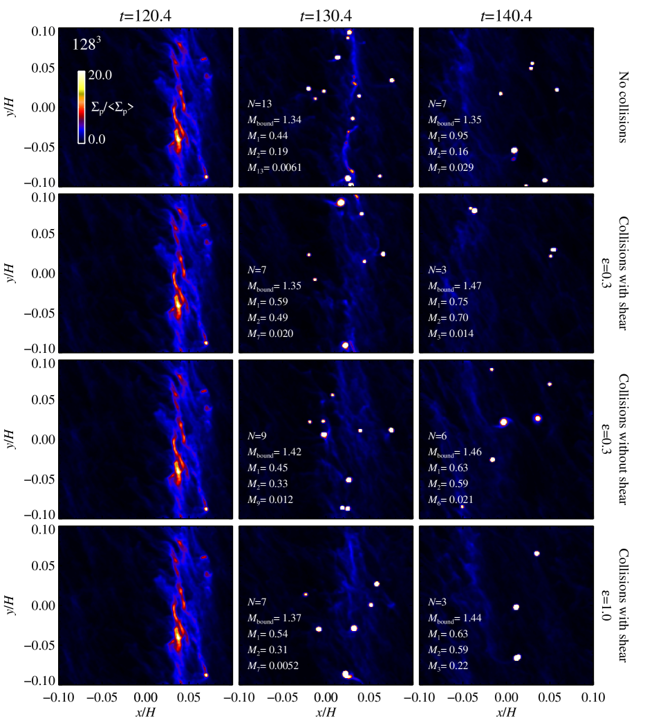
Results at are shown in Fig. 12. At higher resolution the number of clumps condensing out is about twice as high compared to the lower resolution simulation. However, the masses of the most massive clumps are very similar to lower resolution (although a bit higher – up to 60% of Ceres), so it appears that higher resolution simply allows lower-mass clumps to condense out as well. The masses of the clumps condensing out at resolution correspond to contracted radii between 84 and 405 km. The ability to form smaller clumps at higher resolution is expected from the picture that a radial contraction phase is needed before the Roche density can be achieved666A similar order of events is seen in simulations of star formation in self-gravitating accretion discs around supermassive black holes, see e.g. Fig. 3 of Alexander et al. (2008).. Higher resolution allows contraction to narrower bands and thus formation of less massive planetesimals. It is nevertheless difficult to compare the planetesimal masses condensing out at the two resolutions as the initial conditions are not the same.
Rein et al. (2010) observed in their 2-D shearing sheet simulations that inclusion of collisions would lead to condensation of fewer and more massive clumps, when compared to simulations without collisions. Our Fig. 12 also shows that the simulation with no collisions makes the highest number of clumps of all the four simulations. Nevertheless the characteristic mass of the most massive clumps appears indifferent to the treatment of collisions.
Since controls the relative strength of self-gravity, results obtained with a given can not be scaled to other values of . We vary the self-gravity parameter in simulations in Fig. 13, starting self-gravity at the same time as in Fig. 12. Weaker self-gravity gives lower clump masses, but gravitationally bound clumps of up to Ceres masses (or 100 km radius) condense even at . The solar nebula model of Hayashi (1981) has at 3 AU from the sun. Thus the streaming instability allows planetesimal formation in disc models that are similar in mass to the solar nebula, in contrast to recent simulations of planetesimal formation in pressure bumps excited by the magnetorotational instability which required disc masses up to 10 times the solar nebula (Johansen et al., 2011).
The presented simulations do not catch the transition from bound clump to solid planetesimal. However, Nesvorný et al. (2010) simulated the gravitational collapse of spherical particle clouds and generally found formation of binary planetesimals, with the two largest bodies containing a significant fraction of the mass of the cloud. The fact that the masses of the most massive bound clumps in our simulations are relatively independent of resolution allows us to critically compare the mass distribution of the clumps to to the observed properties of the asteroid and Kuiper belts and extrasolar debris discs.
5.1 Application to the Kuiper belt
The physical mass of the clumps depends on location in the disc and on the self-gravity parameter . While the simulations are dimensionless, the translation to physical mass involves multiplication by the mass unit . In a nebula with constant and , the mass unit scales as , so re-scaling to the Kuiper belt777The orbits of trans-Neptunian objects extend to several 10 AU beyond the orbit of Neptune, although many of these must have formed within the orbit of Neptune and been scattered outwards later. Thus we take 30 AU as an approximate distance scale. gives planetesimal masses 5–6 times higher than in Fig. 11 and Fig. 12. Contracted radii at the location of the Kuiper belt are approximately 80% higher than in the asteroid belt, yielding planetesimal radii between 150 and 730 km. The upper range is comparable to the masses of the largest known Kuiper belt objects (Chiang et al., 2007; Brown, 2008).
This extrapolation is only valid for an assumed constant self-gravity parameter . The minimum mass solar nebula, with , has . The weak dependence on radial distance from the star gives in the Kuiper belt at a times larger than in the asteroid belt. From Fig. 13 we read off an approximate doubling in planetesimal mass when increasing from to . We expect that this scaling holds for larger as well. This way the minimum mass solar nebula gives somewhat higher masses in the Kuiper belt compared to the constant- extrapolation presented above.
The comparison to observed planetesimal belts is nevertheless complicated by a potentially very efficient accretion of unbound particles (pebbles and rocks) by the newly born planetesimals after their formation (Johansen & Lacerda, 2010; Ormel & Klahr, 2010), an epoch not captured in our simulations. It is interesting to note that, given the power of the streaming instability in producing Ceres-mass planetesimals from pebbles and rocks, the challenging question may not be how these planetesimal belts form888This does require sufficient amounts of pebbles and rocks to begin with, the formation of which is not yet well-understood (Blum & Wurm, 2008). or how the characteristic mass arises, but rather why the planetesimals did not immediately continue to grow towards terrestrial planets, super-Earths, and cores of ice and gas giants. Perhaps these planetesimal bursts were “abandoned” by the particle overdensity from which they formed, by radial drift of the particles, stranding as planetesimal belts. Such stranding is evident in the last frames of Fig. 11 and Fig. 12 where the gravitationally bound clumps clearly lag behind the overdense particle filament. The lag might have be even more pronounced if the particle clumps would not be bloated to fill a grid cell.
This stranding scenario is an alternative to the more classical view that the asteroid and Kuiper belts were disturbed by the presence of giant planets (e.g. Kenyon & Bromley, 2004).
6 Summary and discussion
This paper focuses on the effect of momentum exchange and energy dissipation in collisions on particle concentration by the streaming instability and on the subsequent gravitational collapse to form dense clumps and planetesimals. We develop a new algorithm for tracking collisions between superparticles representing swarms of physical particles. The time-scale for a particle in a given swarm to collide with a particle from another swarm is calculated for all superparticle pairs in a grid cell. Collisions occur instantaneously if a random number is less than the ratio of the simulation time-step to the collisional time-scale, ensuring that superparticles collide statistically on the correct time-scale. We have demonstrated that this algorithm can be incorporated into a hydrodynamical code at a modest computational cost. This is true even for large particle numbers, since the number of possible collision partners that are considered in a given timestep can be reduced with little or no loss of generality.
Collisions can have a number of effects on particle dynamics, by making particle motion more isotropic and by dissipative collisions which drain kinetic energy from the system. We have considered the simplest case of a constant coefficient of restitution (either unity or 0.3), but a more physically motivated coefficient of restitution, depending on material properties and impact speed and angle, could be easily implemented in the scheme. We emphasize that we have focused in this paper entirely on particles with a friction time of 0.3 relative to the local Keplerian time-scale, corresponding to 20-cm rocks in the asteroid belt and 6-mm pebbles at 30 AU. Future studies will be needed to determine the influence of particle collisions on the dynamics of smaller and larger particles and on their ability to form planetesimals.
Our simulations show that collisions are important to consider when modelling particle concentration by the streaming instability. Taking into account the energy dissipation in inelastic collisions increases the maximum particle density. This increase is most pronounced, more than a factor of three compared to simulations with no collisions, when we ignore the relative Keplerian shear for determining the collision time-scales and outcomes. We argue that the Keplerian shear velocity should be subtracted when determining the outcome of collisions between superparticles representing physical particles that are much smaller than a grid cell. The collision algorithm enlarges particles to the size of a grid cell during a collision, and this can lead to unphysical heating of the particle component if the Keplerian shear is included during the collision.
The treatment of collisions has no apparent effect on the planetesimals which form by self-gravity. The masses of the most massive planetesimals are relatively independent of the inclusion or absence of collisions, although we find some evidence that more low-mass clumps condense out in simulations without collisions. The particle densities reach several hundred and even thousand times the gas density both with and without collisions – much higher than the Roche density which governs gravitational collapse – and that may explain why particle collisions play a relatively small role in determining the outcome of the gravitational contraction to form planetesimals. The simulations show a characteristic planetesimal mass-scale comparable to the dwarf planet Ceres at the location of the asteroid belt. The mass-scale increases approximately linearly with distance from the central star, giving almost double the contracted radius at the distance of the Kuiper belt. This scaling may explain why the largest Kuiper belt objects are bigger than the largest asteroids.
Particle collisions are also important as a stepping stone towards implementing coagulation and fragmentation in planetesimal formation models (Ormel & Spaans, 2008; Zsom & Dullemond, 2008). Including all the physics relevant for modelling particle-dominated self-gravitating flows is a major task, but the reward will be a much better understanding of the important step from pebbles and rocks to planetesimals and dwarf planets.
Acknowledgements.
Y.L. acknowledges support from NSF grant AST-1109776. Computer simulations were performed at the Platon system of the Lunarc Center for Scientific and Technical Computing at Lund University. We are grateful to Hanno Rein, Geoffroy Lesur, Zoe Leinhardt, Yuri Levin, Ross Church, Andras Zsom and Kees Dullemond for stimulating discussions. We thank the referee, Chris Ormel, for raising many interesting points in his very thorough referee report. We thank the Isaac Newton Institute for Mathematical Sciences for providing an environment for stimulating discussions during the “Dynamics of Discs and Planets” programme.References
- Alexander et al. (2008) Alexander, R. D., Armitage, P. J., & Cuadra, J. 2008, MNRAS, 389, 1655
- Bai & Stone (2010a) Bai, X.-N., & Stone, J. M. 2010a, ApJS, 190, 297
- Bai & Stone (2010b) Bai, X.-N., & Stone, J. M. 2010b, ApJ, 722, 1437
- Bai & Stone (2010c) Bai, X.-N., & Stone, J. M. 2010c, ApJ, 722, L220
- Balsara et al. (2009) Balsara, D. S., Tilley, D. A., Rettig, T., & Brittain, S. D. 2009, MNRAS, 397, 24
- Blum & Wurm (2008) Blum, J., & Wurm, G. 2008, ARA&A, 46, 21
- Brown (2008) Brown M. E., 2008, The Largest Kuiper Belt Objects, ed. M. A. Barucci, H. Boehnhardt, D. P. Cruikshank, & A. Morbidelli, 335
- Chiang et al. (2007) Chiang E., Lithwick Y., Murray-Clay R., Buie M., Grundy W., Holman M., 2007, in Protostars and Planets V, ed. B. Reipurth, D. Jewitt, K. Keil, 895
- Chiang & Youdin (2010) Chiang, E., & Youdin, A. N. 2010, Annual Review of Earth and Planetary Sciences, 38, 493
- Dominik & Nübold (2002) Dominik, C., Nübold, H. 2002, Icarus, 157, 173
- Goldreich & Tremaine (1978) Goldreich, P., & Tremaine, S. D. 1978, Icarus, 34, 227
- Goldreich et al. (2004) Goldreich, P., Lithwick, Y., & Sari, R. 2004, ARA&A, 42, 549
- Goodman & Pindor (2000) Goodman, J., & Pindor, B. 2000, Icarus, 148, 537
- Hayashi (1981) Hayashi, C. 1981, Progress of Theoretical Physics Supplement, 70, 35
- Heißelmann et al. (2010) Heißelmann, D., Blum, J., Fraser, H. J., & Wolling, K. 2010, Icarus, 206, 424
- Higa et al. (1996) Higa, M., Arakawa, M., & Maeno, N. 1996, Planet. Space Sci., 44, 917
- Hogan & Cuzzi (2007) Hogan, R. C., & Cuzzi, J. N. 2007, Physical Review E, 75, 056305
- Johansen et al. (2007) Johansen, A., Oishi, J. S., Low, M.-M. M., Klahr, H., Henning, T., & Youdin, A. N. 2007, Nature, 448, 1022
- Johansen & Youdin (2007) Johansen, A., & Youdin, A. N. 2007, ApJ, 662, 627
- Johansen et al. (2009) Johansen, A., Youdin, A. N., & Mac Low, M.-M. 2009, ApJ, 704, L75
- Johansen & Lacerda (2010) Johansen, A., & Lacerda, P. 2010, MNRAS, 404, 475
- Johansen et al. (2011) Johansen, A., Klahr, H., & Henning, T. 2011, A&A, 529, A62
- Karjalainen & Salo (2004) Karjalainen, R., & Salo, H. 2004, Icarus, 172, 328
- Kenyon & Bromley (2004) Kenyon, S. J., & Bromley, B. C. 2004, AJ, 128, 1916
- Kenyon & Bromley (2010) Kenyon, S. J., & Bromley, B. C. 2010, ApJS, 188, 242
- Kokubo & Ida (1996) Kokubo, E., & Ida, S. 1996, Icarus, 123, 180
- Krivov (2010) Krivov, A. V. 2010, Research in Astronomy and Astrophysics, 10, 383
- Lee et al. (2010) Lee, A. T., Chiang, E., Asay-Davis, X., & Barranco, J. 2010, ApJ, 725, 1938
- Lithwick & Chiang (2007) Lithwick, Y., & Chiang, E. 2007, ApJ, 656, 524
- Lyra et al. (2009) Lyra, W., Johansen, A., Zsom, A., Klahr, H., & Piskunov, N. 2009, A&A, 497, 869
- Michikoshi et al. (2007) Michikoshi, S., Inutsuka, S., Kokubo, E., & Furuya, I. 2007, ApJ, 657, 521
- Michikoshi et al. (2010) Michikoshi, S., Kokubo, E., & Inutsuka, S.-i. 2010, ApJ, 719, 1021
- Miniati (2010) Miniati, F. 2010, Journal of Computational Physics, 229, 3916
- Morbidelli et al. (2009) Morbidelli, A., Bottke, W. F., Nesvorný, D., & Levison, H. F. 2009, Icarus, 204, 558
- Nakagawa et al. (1986) Nakagawa, Y., Sekiya, M., & Hayashi, C. 1986, Icarus, 67, 375
- Nesvorný et al. (2010) Nesvorný, D., Youdin, A. N., & Richardson, D. C. 2010, AJ, 140, 785
- Ormel & Spaans (2008) Ormel, C. W., & Spaans, M. 2008, ApJ, 684, 1291
- Ormel & Klahr (2010) Ormel, C. W., & Klahr, H. H. 2010, A&A, 520, A43
- Pan et al. (2011) Pan, L., Padoan, P., Scalo, J., Kritsuk, A. G., & Norman, M. L. 2011, arXiv:1106.3695
- Petit & Henon (1987) Petit, J., & Henon, M. 1987, A&A, 188, 198
- Rein et al. (2010) Rein, H., Lesur, G., & Leinhardt, Z. M. 2010, A&A, 511, A69
- Safronov (1960) Safronov, V. S. 1960, Annales d’Astrophysique, 23, 979
- Safronov (1969) Safronov, V. S. 1969, Evoliutsiia doplanetnogo oblaka. (English transl.: Evolution of the Protoplanetary Cloud and Formation of Earth and the Planets, NASA Tech. Transl. F-677, Jerusalem: Israel Sci. Transl. 1972)
- Salo (1991) Salo, H. 1991, Icarus, 90, 254
- Shariff & Cuzzi (2011) Shariff, K., & Cuzzi, J. N. 2011, ApJ, 738, 73
- Sheppard & Trujillo (2010) Sheppard, S. S., & Trujillo, C. A. 2010, ApJ, 723, L233
- Shu (1977) Shu, F. H. 1977, ApJ, 214, 488
- Toomre (1964) Toomre, A. 1964, ApJ, 139, 1217
- Weidenschilling (1977) Weidenschilling, S. J. 1977, MNRAS, 180, 57
- Weidenschilling (2010) Weidenschilling, S. J. 2010, ApJ, 722, 1716
- Wisdom & Tremaine (1988) Wisdom, J., & Tremaine, S. 1988, AJ, 95, 925
- Youdin & Shu (2002) Youdin, A., & Shu, F. H. 2002, ApJ, 580, 494
- Youdin & Goodman (2005) Youdin, A. N., & Goodman, J. 2005, ApJ, 620, 459
- Youdin & Johansen (2007) Youdin, A. N., & Johansen, A. 2007, ApJ, 662, 613
- Youdin (2011) Youdin, A. N. 2011, ApJ, 731, 99
- Zsom & Dullemond (2008) Zsom, A., & Dullemond, C. P. 2008, A&A, 489, 931
Appendix A Collision time from friction time
In connection with the presence of gas it is convenient to express the collision time-scale in terms of the gas friction time-scale. In the Epstein drag force regime, valid when the radius of a particle is smaller than ( times) the mean free path of gas molecules (Weidenschilling, 1977), the friction time-scale is
| (22) |
Here is the material density of the particles, while and are the sound speed and density of the gas molecules.
The time-scale for a particle of radius to collide with a swarm of particles with physical radius is
| (23) |
where is the mutual collisional cross section. Writing further and and assuming spherical particles we arrive at
| (24) |
In terms of the friction time we get
| (25) |
For collisions between equal-sized particles, with , the expression reduces to
| (26) |
A time-dependent numerical solution of a collisional particle system must take collisions into account when choosing the time-step. The time-step criterion of the Monte Carlo collision scheme originates in the requirement that two particles can collide at most once during a time-step, i.e. the collision probability between any two particles in the same grid cell must be much smaller the unity. This time-step is independent of the maximum density in a grid cell, since particles in dense grid cells have many collision partners and hence can suffer more collisions in the same time-step.
In the streaming instability simulations presented in Sect. 4 and Sect. 5 we observe a typical particle rms speed . The mass density represented by a single superparticle is and the friction time is (we normalise here by the Keplerian frequency which we define in Sect. 4). This gives from Eq. (26). The Courant criterion for the hydrodynamical part of the streaming instability gives the time-step for and for simulations. Therefore we can ignore the collision time-scale in the simulations when determining the numerical time-step.
A.1 Multiple particle sizes
Eq. (23) defines the collisional time-scale between particles of two sizes. For two superparticles of equal internal particle number () we have , because the cross section and relative speed are symmetric in . However, equal particle number per superparticle is numerically expensive, as the mass of a superparticle in that case scales as , requiring many more superparticles to represent an equal mass of smaller particles. The second complication is that the collision time-scale becomes very short for smaller particles.
A more common approach is to have equal mass per superparticle. In that case we can define a collision time-scale as the time for all mass in particle to interact with all mass in particle . This time-scale is shared between the two particle species and is given by
| (27) |
To illustrate this, take small particles of friction time and large particles of friction time . The collision time-scale for the large particles is 100 times shorter than for the small particles, because the superparticle with small physical particles contains 100 times more particles in the swarm. However, the time-scale for collision between a large and a small particle does not imply that all small particles have collided during that time. The correct time-scale is the time for small particles to collide with large particles. When an average small particle has experienced a collision, then all small particles have collided with a large particle, and all the mass in the two superparticles have interacted.
After waiting the common collision time , the collision outcome can be solved as if the two colliding particles had equal mass, since effectively a large particle collides with small particles during this time. This approach is slightly inconsistent since discrete collisions with particles of mass is not equal to a single collision with a particle of mass . A collision between a particle of velocity and a stationary particle results in the new velocity
| (28) |
After such collisions the velocity of particle is
| (29) |
In the limit where , this equation describes a velocity damping
| (30) |
with characteristic time-scale . Completely braking down the large particle requires infinite time, whereas a single discrete collision with an equal-mass particle would remove all the momentum from particle in one collision time.
To really get the collisional energy equipartition right between particles of different sizes one would have to allow for collisions between a large particle and individual smaller particles. This could either be done by letting superparticles not represent the same mass, but rather the same number of particles. However, this approach would become unpractical to model a large span in particle sizes, since a huge number of superparticles would be required to represent the low-mass particle bins. Alternatively the collision between a swarm of large and small particles could be modelled on the collision time-scale of individual collisions, distributing afterwards the energy and momentum of the particle that suffered the collision among the entire swarm of small particles or among all particle swarms within its mean free path. However, for a large span in particle sizes, this would still require a very small time-step and is therefore unpractical. We simply note here that while collisions between unequal-sized particles can be modelled with the right conservation properties, actual equipartition of particle energies would require an adaptation of the collision algorithm.
Appendix B Limiting the collision number
During the gravitational contraction of particle clumps the number of particles in a grid cell can become very large, on the order of 1000s of 10000s. Tracking possible collisions per grid cell then becomes very computationally expensive.
However, particles do not collide with all possible partners during a single time-step. One can limit the number of collision partners, while maintaining the overall collision rate, by sampling only a subset of the possible collisions. Considering only out of the collision partners for each particle in a grid cell, while increasing the collision probability for each collision partner by , yields statistically the same number of collisions.
Consider as an example 101 particles in a grid cell, with the collision probability between any two particles of . Particle 1 will then on the average collide with 1 other particle. However, calculating the collision probability with 100 other particles is expensive, even when it does not lead to a collision, which is most often the case. Instead we let particle 1 only interact with particles to , and give each collision the probability instead of . Particle has particles to as collision partners. When reaching particle , the collision partners wrap around to particle 1 again, and this way all particles on the average get 10 collision partners (5 of higher index and 5 of lower index) instead of 100.
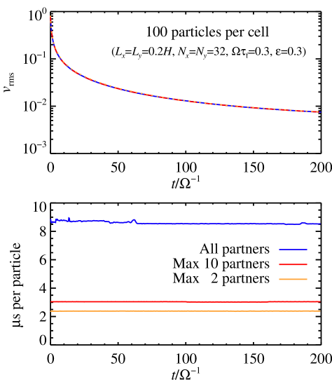
When reducing the number of collision partners, one has to be careful that the particles do not interact only with particles of a nearby index in each time-step. To avoid any such spurious particle preferences, we therefore shuffle the order of particles inside a grid cell in each time-step. We have empirically found that reducing the number of collision partners becomes important when there are more than 100 particles in a grid cell. We show in Fig. 14 the rms speed of particles undergoing inelastic collisions with coefficient of restitution . We use 100 particles per grid cell and show results where we consider all particles in a cell to be collision partners together with results where we limit the collision partners to 10 and 2. The results are indistinguishable, but the code speed is significantly higher when limiting the number of collision partners (lower panel of Fig. 14). The typical speed of the Pencil Code for a hydrodynamical simulation with two-way drag forces between gas and particles is 10 s per particle per time-step. Fig. 14 shows that the computational time needed for superparticle collisions is similar to or lower than the time needed for gas hydrodynamics, particle dynamics, and drag forces, if the number of collision partners is kept below approximately 100.
A side effect of reducing the number of collision partners is that the maximum number of collisions is reduced accordingly. Therefore it be must required that the boosted collision probability is always much smaller than unity. This must hold for all particle pairs. One can use the maximum relative speed between any two particles within a grid cell to estimate the smallest allowed that keeps all .
Each swarm in our simulations represents . The base probability for collision between two superparticle swarms with random motion is using Eq. (26) and a typical hydrodynamical time-step at and resolution. The maximum density reached in the simulations is (see Fig. 7), giving particles in the densest cells. We use and thus the maximum boosted probability is , safely in the regime where the collision time-scale can be ignored when determining the numerical time-step of the code.
Appendix C From superparticles to inflated particles
Consider a particle component of mass density . A superparticle can maximally hold a particle number (equivalently particle mass density ) that covers the whole area of the grid cell,
| (31) |
Here is the cross section of a swarm member and is the mean free path of physical particles in the system. This gives a maximum superparticle mass density of
| (32) |
At this mass density the Monte Carlo method breaks down because the superparticle area is larger than a single grid cell (this is not taken into account in the model because collisions are only considered when superparticles share the same grid cell). The free path of a test particle encountering this maximum density superparticle is
| (33) |
using . Thus the maximum area criterion coincides with the particle density where the free path is the same as the grid spacing, giving a collision probability of unity when the particle enters a grid cell occupied by a superparticle. This is in fact equivalent to the inflated particle approach, i.e. that overlapping particles always collide.
We still must show that the mean free path of the system is equal to the physical mean free path. The total particle number in the box is
| (34) |
This gives a mean free path for the “grid point particles” of
| (35) |
This shows how the superparticle Monte Carlo method smoothly transforms to the inflated particle method when reducing the number of superparticles and increasing their mass. At the point when the superparticle fills up its grid cell, the collision probability approaches unity inside the cell and the mean free path of the grid cell particles is equal to the mean free path of the physical particles. At the same time one must only allow approaching particles to collide, to avoid multiple collisions inside the grid cell. Of course, the collision detection algorithm for these cubic particles is rather crude, but the geometric effect of considering cubic rather than spherical particles is minor.