Optimization of Convex Functions with Random Pursuit

Abstract

We consider unconstrained randomized optimization of convex objective functions. We analyze the Random Pursuit algorithm, which iteratively computes an approximate solution to the optimization problem by repeated optimization over a randomly chosen one-dimensional subspace. This randomized method only uses zeroth-order information about the objective function and does not need any problem-specific parametrization. We prove convergence and give convergence rates for smooth objectives assuming that the one-dimensional optimization can be solved exactly or approximately by an oracle. A convenient property of Random Pursuit is its invariance under strictly monotone transformations of the objective function. It thus enjoys identical convergence behavior on a wider function class. To support the theoretical results we present extensive numerical performance results of Random Pursuit, two gradient-free algorithms recently proposed by Nesterov, and a classical adaptive step-size random search scheme. We also present an accelerated heuristic version of the Random Pursuit algorithm which significantly improves standard Random Pursuit on all numerical benchmark problems. A general comparison of the experimental results reveals that (i) standard Random Pursuit is effective on strongly convex functions with moderate condition number, and (ii) the accelerated scheme is comparable to Nesterov’s fast gradient method and outperforms adaptive step-size strategies.

1 Introduction

Randomized zeroth-order optimization schemes were among the first algorithms proposed to numerically solve unconstrained optimization problems [1, 6, 34]. These methods are usually easy to implement, do not require gradient or Hessian information about the objective function, and comprise a randomized mechanism to iteratively generate new candidate solutions. In many areas of modern science and engineering such methods are indispensable in the simulation (or black-box) optimization context, where higher-order information about the simulation output is not available or does not exist. Compared to deterministic zeroth-order algorithms such as direct search methods [21] or interpolation methods [8] randomized schemes often show faster and more robust performance on ill-conditioned benchmark problems [2] and certain real-world applications such as quantum control [5] and parameter estimation in systems biology networks [39]. While probabilistic convergence guarantees even for non-convex objectives are readily available for many randomized algorithms [41], provable convergence rates are often not known or unrealistically slow. Notable exceptions can be found in the literature on adaptive step size random search (also known as Evolution Strategies) [4, 14], on Markov chain methods for volume estimation, rounding, and optimization [40], and in Nesterov’s recent work on complexity bounds for gradient-free convex optimization [29].

Although Nesterov’s algorithms are termed “gradient-free” their working mechanism does, in fact, rely on approximate directional derivatives that have to be available via a suitable oracle. We here relax this requirement and investigate a true randomized gradient- and derivative-free optimization algorithm: Random Pursuit ($\mathcal{RP}_{\mu}$). The method comprises two very elementary primitives: a random direction generator and an (approximate) line search routine. We establish theoretical performance bounds of this algorithm for the unconstrained convex minimization problem

$$\min f(x)\quad\text{subject to}\quad x\in\mathbb{R}^{n}\,,$$ (1)

where $f$ is a smooth convex function. We assume that there is a global minimum and that the curvature of the function $f$ can bounded by a constant. Each iteration of Random Pursuit consists of two steps: A random direction is sampled uniformly at random from the unit sphere. The next iterate is chosen such as to (approximately) minimize the objective function along this direction. This method ranges among the simplest possible optimization schemes as it solely relies on two easy-to-implement primitives: a random direction generator and an (approximate) one-dimensional line search. A convenient feature of the algorithm is that it inherits the invariance under strictly monotone transformations of the objective function from the line search oracle. The algorithm thus enjoys convergence guarantees even for non-convex objective functions that can be transformed into convex objectives via a suitable strictly monotone transformation.

Although Random Pursuit is fully gradient- and derivative-free, it can still be understood from the perspective of the classical gradient method. The gradient method ($\mathcal{GM}$) is an iterative algorithm where the current approximate solution $x_{k}\in\mathbb{R}^{n}$ is improved along the direction of the negative gradient with some step size $\lambda_{k}$:

$$x_{k+1}=x_{k}+\lambda_{k}(-\nabla f(x_{k}))\,.$$ (2)

When the descent direction is replaced by a random vector the generic scheme reads

$$x_{k+1}=x_{k}+\lambda_{k}u\,,$$ (3)

where $u$ is a random vector distributed uniformly over the unit sphere. A crucial aspect of the performance of this randomized scheme is the determination of the step size. Rastrigin [34] studied the convergence of this scheme on quadratic functions for fixed step sizes $\lambda_{k}$ where only improving steps are accepted. Many authors observed that variable step size methods yield faster convergence [24, 18]. Schumer and Steiglitz [36] were among the first to develop an effective step size adaptation rule which is based on the maximization of the expected one-step progress on the sphere function. A similar analysis has been independently obtained by Rechenberg for the (1+1)-Evolution Strategy ($\mathcal{ES}$) [35]. Mutseniyeks and Rastrigin proposed to choose the step size such as to minimize the function value along the random direction [26]. This algorithm is identical to Random Pursuit with an exact line search. Convergence analyses on strongly convex functions have been provided by Krutikov [22] and Rappl [33]. Rappl proved linear convergence of $\mathcal{RP}_{\mu}$ without giving exact convergence rates. Krutikov showed linear convergence in the special case where the search directions are given by $n$ linearly independent vectors which are used in cyclic order.

Karmanov [16, 17, 42] already conducted an analysis of Random Pursuit on general convex functions. Thus far, Karmanov’s work has not been recognized by the optimization community but his results are very close to the work presented here. We enhance Karmanov’s results in a number of ways: (i) we prove expected convergence rates also under approximate line search; (ii) we show that continuous sampling from the unit sphere can be replaced with discrete sampling from the set $\{\pm e_{i}:i=1,\ldots,n\}$ of signed unit vectors, without changing the expected convergence rates; (iii) we provide a large number of experimental results, showing that Random Pursuit is a competitive algorithm in practice; (iv) we introduce a heuristic improvement of Random Pursuit that is even faster on all our benchmark functions; (v) we point out that Random Pursuit can also be applied to a number of relevant non-convex functions, without sacrificing any theoretical and practical performance guarantees. On the other hand, while we prove fast convergence only in expectation, Karmanov’s more intricate analysis also yields fast convergence with high probability.

Polyak  [31] describes step size rules for the closely related randomized gradient descent scheme:

$$x_{k+1}=x_{k}+\lambda_{k}\frac{f(x_{k}+\mu_{k}u)-f(x_{k})}{\mu_{k}}u\,,$$ (4)

where convergence is proved for $\mu_{k}\to 0$ but no convergence rates are established. Nesterov [29] studied different variants of method (4) and its accelerated versions for smooth and non-smooth optimization problems. He showed that scheme (4) is at most $O(n^{2})$ times slower than the standard (sub-)gradient method. The use of exact directional derivatives reduces the gap further to $O(n)$. For smooth problems the method is only $O(n)$ slower than the standard gradient method and accelerated versions are $O(n^{2})$ slower than fast gradient methods.

Kleiner et al. [20] studied a variant of algorithm (3) for unconstrained semidefinite programming: Random Conic Pursuit. There, each iteration comprises two steps: (i) the algorithm samples a rank-one matrix (not necessarily uniformly) at random; (ii) a two-dimensional optimization problem is solved that consists of finding the optimal linear combination of the rank-one matrix and the current semidefinite matrix. The solution determines the next iterate of the algorithm. In the case of trace-constrained semidefinite problems only a one-dimensional line search is necessary. Kleiner and co-workers proved convergence of this algorithm when directions are chosen uniformly at random. The dependency between convergence rate and dimension are, however, not known. Nonetheless, their work greatly inspired our own efforts which is also reflected in the name “Random Pursuit” for the algorithm under study.

The present article is structured as follows. In Section 2 we present the Random Pursuit algorithm with approximate line search. We introduce the necessary notation and formulate the assumptions on the objective function. In Section 3 we derive a number of useful results on the expectation of scaled random vectors. In Section 4 we calculate the expected one-step progress of Random Pursuit with approximate line search ($\mathcal{RP}_{\mu}$). We show that (besides some additive error term) this progress is by a factor of $O(n)$ worse than the one-step progress of the gradient method. These results allow us to derive the final convergence results in Section 5. We show that $\mathcal{RP}_{\mu}$ meets the convergence rates of the standard gradient method up to a factor of $O(n)$, i.e., linear convergence on strongly convex functions and convergence rate $1/k$ for general convex functions. The linear convergence on strongly convex functions is best possible: For the sphere function our method meets the lower bound [15]. For strongly convex objective functions the method is robust against small absolute or relative errors in the line search. In Section 6 we present numerical experiments on selected test problems. We compare $\mathcal{RP}_{\mu}$ with a fixed step size gradient method and a gradient scheme with line search, Nesterov’s random gradient scheme and its accelerated version [29], an adaptive step size random search, and an accelerated heuristic version of $\mathcal{RP}_{\mu}$. In Section 7 we discuss the theoretical and numerical results as well as the present limitations of the scheme that may be alleviated by more elaborate randomization primitives. We also provide a number of promising future research directions.

2 The Random Pursuit (RP) Algorithm

We consider problem (1) where $f$ is a differentiable convex function with bounded curvature (to be defined below). The algorithm $\mathcal{RP}_{\mu}$ is a variant of scheme (3) where the step sizes are determined by a line search. Formally, we define the following oracles:

Definition 1 (Line search oracle).

For $x\in\mathbb{R}^{n}$, a convex function $f$, and a direction $u\in S^{n-1}=\{y\in\mathbb{R}^{n}\colon\left\lVert y\right\rVert_{2}=1\}$, a function $\text{{LS}}\colon\mathbb{R}^{n}\times S^{n-1}\to\mathbb{R}$ with

$$\text{{LS}}(x,u)\in\displaystyle\arg\min_{h\in\mathbb{R}}f(x+hu)$$ (5)

is called an exact line search oracle. (Here, the $\arg\min$ is not assumed to be unique, so we consider it as a set from which $\text{{LS}}(x,u)$ selects a well-defined element.) For accuracy $\mu\geq 0$ the functions $\text{{LSapprox}}^{\text{rel}}_{\mu}$ and $\text{{LSapprox}}^{\text{abs}}_{\mu}$ with

$$\text{{LS}}(x,u)-\mu\leq\text{{LSapprox}}^{\text{abs}}_{\mu}(x,u)\leq\text{{LS}}(x,u)+\mu,\quad\text{and},$$ (6)

$$s\cdot\max\{0,(1-\mu)\}\cdot\text{{LS}}(x,u)\leq s\cdot\text{{LSapprox}}^{\text{rel}}_{\mu}(x,u)\leq s\cdot\text{{LS}}(x,u),$$ (7)

where $s=\operatorname{sign}(\text{{LS}}(x,u))$, are, respectively, absolute and relative, approximate line search oracles. By $\texttt{{LSapprox}}_{\mu}$, we denote any of the two.

This means that we allow an inexact line search to return a value $\tilde{h}$ close to an optimal value $h^{*}=\text{{LS}}(x,u)$. To simplify subsequent calculations, we also require that $\tilde{h}\leq h^{*}$ in the case of relative approximation (cf. (7)), but this requirement is not essential. As the optimization problem (5) cannot be solved exactly in most cases, we will describe and analyze our algorithm by means of the two latter approximation routines.

The formal definition of algorithm $\mathcal{RP}_{\mu}$ is shown in Algorithm 1. At iteration $k$ of the algorithm a direction $u\in S^{n-1}$ is chosen uniformly at random and the next iterate $x_{k+1}$ is calculated from the current iterate $x_{k}$ as

$$x_{k+1}:=x_{k}+\texttt{{LSapprox}}_{\mu}(x_{k},u)\cdot u.$$ (8)

Algorithm 1 Random Pursuit ($\mathcal{RP}_{\mu}$)

0:  $\begin{array}[]{ll}\text{A problem of the form~{}\eqref{eq:problem}}&N\in\mathbb{N}:\text{number of iterations}\\ x_{0}:\text{an initial iterate}&\mu>0:\text{line search accuracy}\end{array}$

0:  Approximate solution $x_{N}$ to (1).

1:  for $k\leftarrow 0$ to $N-1$ do

2:        choose $u_{k}$ uniformly at random from $S^{n-1}$

3:        Set $x_{k+1}\leftarrow x_{k}+\texttt{{LSapprox}}_{\mu}(x_{k},u_{k})\cdot u_{k}$

4:  end for

5:  return  $x_{N}$

This algorithm only requires function evaluations if the line search $\texttt{{LSapprox}}_{\mu}$ is implemented appropriately (see [9] and references therein). No additional first or second-order information of the objective is needed. Note also that besides the starting point no further input parameters describing function properties (e.g. curvature constant, etc.) are necessary. The actual run time will, however, depend on the specific properties of the objective function.

2.1 Discrete Sampling

As our analysis below reveals, the random vector $u_{k}$ enters the analysis only in terms of expectations of the form $\operatorname{\mathbb{E}}[\left\langle x,u_{k}\right\rangle u_{k}]$ and $\operatorname{\mathbb{E}}[\left\lVert\left\langle x,u_{k}\right\rangle u_{k}\right\rVert^{2}]$. In Lemmas 4 and 5 we show that these expectations are the same for $u_{k}\sim S^{n-1}$ and $u_{k}\sim\{\pm e_{i}:i=1,\ldots,n\}$, the set of signed unit vectors (here and in the following, the notation $x\sim A$ for a set $A$, denotes that $x$ is distributed according to the uniform distribution on $A$). It follows that continuous sampling from $S^{n-1}$ can be replaced with discrete sampling from $\{\pm e_{i}:i=1,\ldots,n\}$ without affecting our guarantees on the expected runtime. Under this modification, fast convergence still holds with high probability, but the bounds get worse [17].

2.2 Quasiconvex Functions

If $f$ and $g$ are functions, $g$ is called a strictly monotone transformation of $f$ if

$$f(x)<f(y)~{}~{}\Leftrightarrow~{}~{}g(f(x))<g(f(y)),\quad x,y\in\mathbb{R}^{n}.$$

This implies that the distribution of $x_{k}$ in $\mathcal{RP}_{\mu}$ is the same for the function $f$ and the function $g\circ f$, if $g$ is a strictly monotone transformation of $f$. This follows from the fact that the result of the line search given in Definition 1 is invariant under strictly monotone transformations.

This observation allows us to run $\mathcal{RP}_{\mu}$ on any strictly monotone transformation of any convex function $f$, with the same theoretical performance as on $f$ itself. The functions obtainable in this way form a subclass of the class of quasiconvex functions, and they include some non-convex functions as well. In Section 6.2.3 we will experimentally verify the invariance of $\mathcal{RP}_{\mu}$ under strictly monotone transformations on one instance of a quasiconvex function.

2.3 Function Basics

We now introduce some important inequalities that are useful for the subsequent analysis. We always assume that the objective function is differentiable and convex. The latter property is equivalent to

$$f(y)\geq f(x)+\left\langle\nabla f(x),y-x\right\rangle,\quad x,y\in\mathbb{R}^{n}\,.$$ (9)

We also require that the curvature of $f$ is bounded. By this we mean that for some constant $L_{1}$,

$$f(y)-f(x)-\left\langle\nabla f(x),y-x\right\rangle\leq\frac{1}{2}L_{1}\left\lVert x-y\right\rVert^{2},\quad x,y\in\mathbb{R}^{n}\,.$$ (10)

We will also refer to this inequality as the quadratic upper bound. It means that the deviation of $f$ from any of its linear approximations can be bounded by a quadratic function. We denote by $C^{1}_{L_{1}}$ the class of differentiable and convex functions for with the quadratic upper bound holds with the constant $L_{1}$.

A differentiable function is strongly convex with parameter $m$ if the quadratic lower bound

$$f(y)-f(x)-\left\langle\nabla f(x),y-x\right\rangle\geq\frac{m}{2}\left\lVert y-x\right\rVert^{2}\,,\quad x,y\in\mathbb{R}^{n}\,,$$ (11)

holds. Let $x^{*}$ be the unique minimizer of a strongly convex function $f$ with parameter $m$. Then equation (11) implies this useful relation:

$$\frac{m}{2}\left\lVert x-x^{*}\right\rVert^{2}\leq f(x)-f(x^{*})\leq\frac{1}{2m}\|\nabla f(x)\|^{2}\,,\quad\forall x\in\mathbb{R}^{n}\,.$$ (12)

The former inequality uses $\nabla f(x^{*})=0$, and the latter one follows from (11) via

$$f(x^{*}) \geq f(x)+\left\langle\nabla f(x),x^{*}-x\right\rangle+\frac{m}{2}\left\lVert x^{*}-x\right\rVert^{2}$$

$$\geq f(x)+\min_{y\in\mathbb{R}^{n}}\left(\left\langle\nabla f(x),y-x\right\rangle+\frac{m}{2}\left\lVert y-x\right\rVert^{2}\right)=f(x)-\frac{1}{2m}\|\nabla f(x)\|^{2}$$

by standard calculus.

3 Expectation of Scaled Random Vectors

We now study the projection of a fixed vector $x$ onto a random vector $u$. This will help analyze the expected progress of Algorithm 1. We start with the case $u\sim\mathcal{N}(0,I_{n})$ and then extend it to $u\sim S^{n-1}$. Throughout this section, let $x\in\mathbb{R}^{n}$ be a fixed vector and $u\in\mathbb{R}^{n}$ a random vector drawn according to some distribution. We will need the following facts about the moments of the standard normal distribution.

Lemma 2.

• Let $\nu\sim\mathcal{N}(0,1)$ be drawn from the standard normal distribution over the reals. Then

  $$\operatorname{\mathbb{E}}[\nu] =\operatorname{\mathbb{E}}[\nu^{3}]=0\,, \operatorname{\mathbb{E}}[\nu^{2}] =1\,, \operatorname{\mathbb{E}}[\nu^{4}] =3\,.$$

• Let $u\sim\mathcal{N}(0,I_{n})$ be drawn from the standard normal distribution over $\mathbb{R}^{n}$. Then

  $$\operatorname{\mathbb{E}}_{u}[uu^{T}] =I_{n}\,, \operatorname{\mathbb{E}}_{u}[(u^{T}u)uu^{T}] =(n+2)I_{n}\,.$$

Proof. Part (i) is standard, and the latter two matrix equations easily follow from (i) via

$$(uu^{T})_{ij} =u_{i}u_{j}\,, \left((u^{T}u)uu^{T}\right)_{ij} =u_{i}u_{j}\sum_{k}u_{k}^{2}\,.\qquad\end@proof$$

Lemma 3 (Normal distribution).

Let $u\sim\mathcal{N}(0,I_{n})$. Then

$$\operatorname{\mathbb{E}}_{u}\left[\left\langle x,u\right\rangle u\right]=x\,,\quad \text{and}\quad\operatorname{\mathbb{E}}_{u}\left[\left\lVert\left\langle x,u\right\rangle u\right\rVert^{2}\right]=(n+2)\left\lVert x\right\rVert^{2}\,.$$

Proof.

We calculate

$$\operatorname{\mathbb{E}}_{u}\left[\left\langle x,u\right\rangle u\right]=\operatorname{\mathbb{E}}_{u}[uu^{T}x]=\operatorname{\mathbb{E}}_{u}[uu^{T}]x=x,$$

by Lemma 2(ii). For the second moment we get

$$\operatorname{\mathbb{E}}_{u}\left[\left\lVert\left\langle x,u\right\rangle u\right\rVert^{2}\right]=\operatorname{\mathbb{E}}_{u}[x^{T}(u^{T}u)uu^{T}x]=x^{T}\operatorname{\mathbb{E}}_{u}[(u^{T}u)uu^{T}]x=(n+2)\left\lVert x\right\rVert^{2}\,,$$

again using Lemma 2(ii). ∎

Lemma 4 (Spherical distribution).

Let $u\sim S^{n-1}$. Then

$$\operatorname{\mathbb{E}}_{u}\left[\left\langle x,u\right\rangle u\right]=\frac{1}{n}x\,,\quad \text{and}\quad\operatorname{\mathbb{E}}_{u}\left[\left\lVert\left\langle x,u\right\rangle u\right\rVert^{2}\right]=\operatorname{\mathbb{E}}_{u}\left[\left\langle x,u\right\rangle^{2}\right]=\frac{1}{n}\left\lVert x\right\rVert^{2}\,.$$

Proof. Let $v\sim\mathcal{N}(0,I_{n})$. We observe that the random vector $w=v/\left\lVert v\right\rVert$ has the same distribution as $u$. In particular,

$$\operatorname{\mathbb{E}}_{u}\left[uu^{T}\right]=\operatorname{\mathbb{E}}_{v}\left[\frac{vv^{T}}{\left\lVert v\right\rVert^{2}}\right]=\frac{\operatorname{\mathbb{E}}_{v}\left[vv^{T}\right]}{\operatorname{\mathbb{E}}_{v}\left[\left\lVert v\right\rVert^{2}\right]}=\frac{I_{n}}{n}\,,$$ (13)

where we have used that the two random variables $\frac{vv^{T}}{\left\lVert v\right\rVert^{2}}$ and $\left\lVert v\right\rVert^{2}$ are independent (see [11]), along with

$$\operatorname{\mathbb{E}}_{v}\left[vv^{T}\right]=I_{n},\quad\operatorname{\mathbb{E}}_{v}\left[\left\lVert v\right\rVert^{2}\right]=n\,,$$

a consequence of Lemma 2. Now we use (13) to compute

$$\operatorname{\mathbb{E}}_{u}\left[\left\langle x,u\right\rangle u\right]=\operatorname{\mathbb{E}}_{u}\left[uu^{T}\right]x=\frac{I_{n}}{n}x=\frac{1}{n}x$$

and

$$\operatorname{\mathbb{E}}_{u}\left[\left\langle x,u\right\rangle^{2}\right] =\operatorname{\mathbb{E}}_{u}\left[x^{T}uu^{T}x\right]=x^{T}\operatorname{\mathbb{E}}_{u}\left[uu^{T}\right]x=x^{T}\frac{I_{n}}{n}x=\frac{1}{n}\left\lVert x\right\rVert^{2}\,.\qquad\end@proof$$

The same result can be derived when the vector $u$ is chosen to be a random signed unit vector.

Lemma 5.

Let $u\sim U:=\{\pm e_{i}:i=1,\ldots,n\}$ where $e_{i}$ denotes the $i$-th standard unit vector in $\mathbb{R}^{n}$. Then

$$\operatorname{\mathbb{E}}_{u}\left[\left\langle x,u\right\rangle u\right]=\frac{1}{n}x\,,\quad \text{and}\quad\operatorname{\mathbb{E}}_{u}\left[\left\lVert\left\langle x,u\right\rangle u\right\rVert^{2}\right]=\operatorname{\mathbb{E}}_{u}\left[\left\langle x,u\right\rangle^{2}\right]=\frac{1}{n}\left\lVert x\right\rVert^{2}.$$

Proof. We calculate

$$\operatorname{\mathbb{E}}_{u}\left[\left\langle x,u\right\rangle u\right]=\frac{1}{2n}\sum_{u\in U}\left\langle x,u\right\rangle u=\frac{1}{n}\sum_{i=1}^{n}x_{i}e_{i}=\frac{1}{n}x\,,$$

and similarly

$$\operatorname{\mathbb{E}}_{u}\left[\left\langle x,u\right\rangle^{2}\right]=\frac{1}{2n}\sum_{u\in U}\left\langle x,u\right\rangle^{2}=\frac{1}{n}\sum_{i=1}^{n}x_{i}^{2}=\frac{1}{n}\left\lVert x\right\rVert^{2}\,.\qquad\end@proof$$

4 Single Step Progress

To prepare the convergence proof of Algorithm $\mathcal{RP}_{\mu}$ in the next section, we study the expected progress in a single step, which is the quantity

$$\operatorname{\mathbb{E}}\left[f(x_{k+1})\mid x_{k}\right]\,.$$

It turns out that we need to proceed differently, depending on whether the function under consideration is strongly convex (the easier case) or not. We start with a preparatory lemma for both cases. We first analyze the case when an approximate line search with absolute error is applied. Using an approximate line search with relative error will be reduced to the case of an exact line search.

4.1 Line Search with Absolute Error

Lemma 6 (Absolute Error).

Let $f\in C^{1}_{L_{1}}$ and let $x_{k}\in\mathbb{R}^{n}$ be the current iterate and $x_{k+1}\in\mathbb{R}^{n}$ the next iterate generated by algorithm $\mathcal{RP}_{\mu}$ with absolute line search accuracy $\mu$. For every positive $h\in\mathbb{R}$ and every point $z\in\mathbb{R}^{n}$ we have

$$\operatorname{\mathbb{E}}\left[f(x_{k+1})\mid x_{k}\right] \leq f(x_{k})+\frac{h}{n}\left\langle\nabla f(x_{k}),z-x_{k}\right\rangle+\frac{L_{1}h^{2}}{2n}\left\lVert z-x_{k}\right\rVert^{2}+\frac{L_{1}\mu^{2}}{2}\,.$$

Proof.

Let $x^{\prime}_{k+1}:=x_{k}+\text{{LS}}(x_{k},u_{k})u_{k}$ be the exact line search optimum. Here, $u_{k}\in S^{n-1}$ is the chosen search direction. By definition of the approximate line search (6), we have

$$f(x_{k+1}) \leq\displaystyle\max_{|\nu|\leq\mu}f(x^{\prime}_{k+1}+\nu u_{k})$$

$$\stackrel{{\scriptstyle(\ref{eq:lipschitz})}}{{\leq}}f(x^{\prime}_{k+1})+\max_{|\nu|\leq\mu}\left[\underbrace{\left\langle\nabla f(x^{\prime}_{k+1}),\nu u_{k}\right\rangle}_{0}+\frac{L_{1}}{2}\nu^{2}\right]$$

$$=f(x^{\prime}_{k+1})+\frac{L_{1}\mu^{2}}{2}\,,$$ (14)

where we used the quadratic upper bound (10) in the second inequality with $x=x^{\prime}_{k+1}$ and $y=x^{\prime}_{k+1}+\nu u_{k}$.

Since $x^{\prime}_{k+1}$ is the exact line search optimum, we in particular have

$$f(x^{\prime}_{k+1})\leq f(x_{k}+t_{k}u_{k})\leq f(x_{k})+\left\langle\nabla f(x_{k}),t_{k}u_{k}\right\rangle+\frac{L_{1}t_{k}^{2}}{2}\,,\quad\forall t_{k}\in\mathbb{R},$$ (15)

where we have applied (10) a second time. Putting together (14) and (15), and taking expectations, we get

$$\operatorname{\mathbb{E}}_{u_{k}}\left[f(x_{k+1})\mid x_{k}\right] \leq f(x_{k})+\operatorname{\mathbb{E}}_{u_{k}}\left[\left\langle\nabla f(x_{k}),t_{k}u_{k}\right\rangle+\frac{L_{1}t_{k}^{2}}{2}\mid x_{k}\right]+\frac{L_{1}\mu^{2}}{2}\,.$$ (16)

Now it is time to choose $t_{k}$ such that we can control the expectations on the right-hand side. We set

$$t_{k}:=h\left\langle z-x_{k},u_{k}\right\rangle,$$

where $h>0$ and $z\in\mathbb{R}^{n}$ are the “free parameters” of the lemma. Via Lemma 4, this entails

$$\operatorname{\mathbb{E}}_{u_{k}}\left[t_{k}u_{k}\right]=\frac{h}{n}(z-x_{k})\,,\quad\operatorname{\mathbb{E}}_{u_{k}}\left[t_{k}^{2}\right]=\frac{h^{2}}{n}\left\lVert z-x_{k}\right\rVert^{2}\,,$$

and the lemma follows. ∎

4.2 Line Search with Relative Error

In the case of relative line search error, we can prove a variant of Lemma 6 with a denominator $n^{\prime}$ slightly larger than $n$. As a result, the analysis under relative line search error reduces to the analysis of exact line search (approximate line search error $0$) in a slightly higher dimension; in the sequel, we will therefore only deal with absolute line search error.

Lemma 7 (Relative Error).

Let $f\in C^{1}_{L_{1}}$ and let $x_{k}\in\mathbb{R}^{n}$ be the current iterate and $x_{k+1}\in\mathbb{R}^{n}$ the next iterate generated by algorithm $\mathcal{RP}_{\mu}$ with relative line search accuracy $\mu$. For every positive $h\in\mathbb{R}$ and every point $z\in\mathbb{R}^{n}$ we have

$$\operatorname{\mathbb{E}}\left[f(x_{k+1})\mid x_{k}\right] \leq f(x_{k})+\frac{h}{n^{\prime}}\left\langle\nabla f(x_{k}),z-x_{k}\right\rangle+\frac{L_{1}h^{2}}{2n^{\prime}}\left\lVert z-x_{k}\right\rVert^{2}\,,$$

where $n^{\prime}=n/(1-\mu)$.

Proof.

By the definition (7) of relative line search error, $x_{k+1}$ is a convex combination of $x_{k}$ and $x^{\prime}_{k+1}$, the exact line search optimum. More precisely, we can compute that

$$x_{k+1}=(1-\gamma)x_{k}+\gamma x^{\prime}_{k+1}\,,$$

where $\gamma\geq 1-\mu$. By convexity of $f$, we thus have

$$f(x_{k+1})\leq(1-\gamma)f(x_{k})+\gamma f(x^{\prime}_{k+1})\leq\mu f(x_{k})+(1-\mu)f(x^{\prime}_{k+1})\,,$$

since $f(x^{\prime}_{k+1})\leq f(x_{k})$. Hence

$$\operatorname{\mathbb{E}}\left[f(x_{k+1})\mid x_{k}\right]\leq\mu f(x_{k})+(1-\mu)\operatorname{\mathbb{E}}\left[f(x^{\prime}_{k+1})\mid x_{k}\right]\,.$$ (17)

Using Lemma 6 with absolute line search error $0$ yields a bound for the latter term:

$$\operatorname{\mathbb{E}}\left[f(x^{\prime}_{k+1})\mid x_{k}\right]\leq f(x_{k})+\frac{h}{n}\left\langle\nabla f(x_{k}),z-x_{k}\right\rangle+\frac{L_{1}h^{2}}{2n}\left\lVert z-x_{k}\right\rVert^{2}\,.$$

Putting this together with (17) yields

$$\operatorname{\mathbb{E}}\left[f(x_{k+1})\mid x_{k}\right]\leq f(x_{k})+(1-\mu)\left(\frac{h}{n}\left\langle\nabla f(x_{k}),z-x_{k}\right\rangle+\frac{L_{1}h^{2}}{2n}\left\lVert z-x_{k}\right\rVert^{2}\right)\,,$$

and with $n^{\prime}=n/(1-\mu)$, the lemma follows. ∎

4.3 Towards the Strongly Convex Case

Here we use $z=x_{k}-\nabla f(x_{k})$ in Lemma 6.

Corollary 8.

Let $f\in C^{1}_{L_{1}}$ and let $x_{k}\in\mathbb{R}^{n}$ be the current iterate and $x_{k+1}\in\mathbb{R}^{n}$ the next iterate generated by algorithm $\mathcal{RP}_{\mu}$ with absolute line search accuracy $\mu$. For any positive $h_{k}\leq\frac{1}{L_{1}}$ it holds that

$$\operatorname{\mathbb{E}}\left[f(x_{k+1})\mid x_{k}\right] \leq f(x_{k})-\frac{h_{k}}{2n}\left\lVert\nabla f(x_{k})\right\rVert^{2}+\frac{L_{1}\mu^{2}}{2}\,.$$

Proof. Lemma 6 with $z=x_{k}-\nabla f(x_{k})$ yields

$$\operatorname{\mathbb{E}}\left[f(x_{k+1})\mid x_{k}\right] \leq f(x_{k})-\frac{h_{k}}{n}\left\langle\nabla f(x_{k}),\nabla f(x_{k})\right\rangle+\frac{L_{1}h_{k}^{2}}{2n}\left\lVert\nabla f(x_{k})\right\rVert^{2}+\frac{L_{1}\mu^{2}}{2}\,.$$

We conclude

$$\operatorname{\mathbb{E}}\left[f(x_{k+1})\mid x_{k}\right]\leq f(x_{k})-\underbrace{\frac{h_{k}}{n}\left(1-\frac{L_{1}h_{k}}{2}\right)}_{\geq\frac{h_{k}}{2n}}\left\lVert\nabla f(x_{k})\right\rVert^{2}+\frac{L_{1}\mu^{2}}{2}\,.\qquad\end@proof$$

4.4 Towards the General Convex Case

For this case, we apply Lemma 6 with $z=x^{*}$.

Corollary 9.

Let $f\in C^{1}_{L_{1}}$ and let $x_{k}\in\mathbb{R}^{n}$ be the current iterate and $x_{k+1}\in\mathbb{R}^{n}$ the next iterate generated by algorithm $\mathcal{RP}_{\mu}$ with absolute line search accuracy $\mu$. Let $x^{*}\in\mathbb{R}^{n}$ be one of the minimizers of the function $f$. For any positive $h_{k}\geq 0$ it holds that

$$\operatorname{\mathbb{E}}\left[f(x_{k+1})-f(x^{*})\mid x_{k}\right] \leq(1-\frac{h_{k}}{n})\left(f(x_{k})-f(x^{*})\right)+\frac{L_{1}h_{k}^{2}}{2n}\left\lVert x^{*}-x_{k}\right\rVert^{2}+\frac{L_{1}\mu^{2}}{2}\,.$$

Proof.

We use Lemma 6 with $z=x^{*}$ and apply convexity (9) to bound the term $\left\langle\nabla f(x_{k}),x^{*}-x_{k}\right\rangle$ from above by $f(x^{*})-f(x_{k})$. Subtracting $f(x^{*})$ from both sides yields the inequality of the corollary. ∎

5 Convergence Results

Here we use the previously derived bounds on the expected single step progress (Corollaries 8 and 9) to show convergence of the algorithm.

5.1 Convergence Analysis for Strongly Convex Functions

We first prove that algorithm $\mathcal{RP}_{\mu}$ converges linearly in expectation on strongly convex functions. Despite strong convexity being a global property, it is sufficient if the function is strongly convex in the neighborhood of its minimizer (see Theorem 11).

Theorem 10.

Let $f\in C^{1}_{L_{1}}$ and let $f$ be strongly convex with parameter $m$, and consider the sequence $\{x_{k}\}_{k\geq 0}$ generated by $\mathcal{RP}_{\mu}$ with absolute line search accuracy $\mu$. Then for any $N\geq 0$, we have

$$\operatorname{\mathbb{E}}\left[f(x_{N})-f(x^{*})\right]\leq\left(1-\frac{m}{L_{1}n}\right)^{N}\left(f(x_{0})-f(x^{*})\right)+\frac{L_{1}^{2}n\mu^{2}}{2m}\,.$$

Proof.

We use Corollary 8 with $h=\frac{1}{L_{1}}$ and the quadratic lower bound to estimate the progress in one step as

$$\operatorname{\mathbb{E}}\left[f(x_{k+1})-f(x^{*})\mid x_{k}\right] \leq f(x_{k})-f(x^{*})-\frac{1}{2nL_{1}}\left\lVert\nabla f(x_{k})\right\rVert^{2}+\frac{L_{1}\mu^{2}}{2}$$

$$\stackrel{{\scriptstyle\eqref{eq:quadraticlower}}}{{\leq}}\left(1-\frac{m}{nL_{1}}\right)\left(f(x_{k})-f(x^{*})\right)+\frac{L_{1}\mu^{2}}{2}\,.$$

After taking expectations (over $x_{k}$), the tower property of conditional expectations yields the recurrence

$$\operatorname{\mathbb{E}}\left[f(x_{k+1})-f(x^{*})\right]\leq\left(1-\frac{m}{nL_{1}}\right)\operatorname{\mathbb{E}}\left[f(x_{k})-f(x^{*})\right]+\frac{L_{1}\mu^{2}}{2}\,.$$

This implies

$$\operatorname{\mathbb{E}}\left[f(x_{N})-f(x^{*})\right]\leq\left(1-\frac{m}{nL_{1}}\right)^{N}\left(f(x_{0})-f(x^{*})\right)+\omega(N)\frac{L_{1}\mu^{2}}{2}\,,$$

with

$$\omega(N):=\sum_{i=0}^{N-1}(1-\frac{m}{L_{1}n})^{i}\leq\frac{L_{1}n}{m}\,.$$

The bound of the theorem follows. ∎

We remark that by strong convexity the error $\left\lVert x_{N}-x^{*}\right\rVert$ can also be bounded using the results of this theorem. Thus, the algorithm does not only converge in terms of function value, but also in terms of the solution itself.

Each strongly convex function has a unique minimizer $x^{*}$. Using the quadratic lower bound (12) we recall that:

$$f(x)-f(x^{*})\geq\frac{m}{2}\left\lVert x-x^{*}\right\rVert^{2},\quad\forall x\in\mathbb{R}^{n}.$$ (18)

It turns out that instead of strong convexity (11) the weaker condition (18) is sufficient to have linear convergence.

Theorem 11.

Let $f\in C^{1}_{L_{1}}$ and suppose $f$ has a unique minimizer $x^{*}$ satisfying (18) with parameter $m$. Consider the sequence $\{x_{k}\}_{k\geq 0}$ generated by $\mathcal{RP}_{\mu}$ with absolute line search accuracy $\mu$. Then for any $N\geq 0$, we have

$$\operatorname{\mathbb{E}}\left[f(x_{N})-f(x^{*})\right]\leq\left(1-\frac{m}{4L_{1}n}\right)^{N}\left(f(x_{0})-f(x^{*})\right)+\frac{2L_{1}^{2}n\mu^{2}}{m}\,.$$

Proof.

To see this we use Corollary 9 with property (18) to get

$$\operatorname{\mathbb{E}}\left[f(x_{k+1})-f(x^{*})\mid x_{k}\right] \leq\left(1-\frac{h_{k}}{n}\right)\left(f(x_{k})-f(x^{*})\right)+\frac{L_{1}h_{k}^{2}}{2n}\left\lVert x_{k}-x^{*}\right\rVert^{2}+\frac{L_{1}\mu^{2}}{2}$$

$$\leq\left(1-\frac{h_{k}}{n}+\frac{L_{1}h_{k}^{2}}{mn}\right)\left(f(x_{k})-f(x^{*})\right)+\frac{L_{1}\mu^{2}}{2}\,.$$

Setting $h_{k}$ to $\frac{m}{2L_{1}}$, the term in the left bracket becomes $(1-\frac{m}{4L_{1}n})$. Now the proof continues as the proof of Theorem 10. ∎

5.2 Convergence Analysis for Convex Functions

We now prove that algorithm $\mathcal{RP}_{\mu}$ converges in expectation on smooth (not necessarily strongly) convex functions. The rate is, however, not linear anymore.

Theorem 12.

Let $f\in C^{1}_{L_{1}}$ and let $x^{*}$ a minimizer of $f$, and let the sequence $\{x_{k}\}_{k\geq 0}$ be generated by $\mathcal{RP}_{\mu}$ with absolute line search accuracy $\mu$. Assume there exists $R$, s.t. $\left\lVert y-x^{*}\right\rVert<R$ for all $y$ with $f(y)\leq f(x_{0})$. Then for any $N\geq 0$, we have

$$\operatorname{\mathbb{E}}\left[f(x_{N})-f(x^{*})\right]\leq\frac{Q}{N+1}+\frac{NL_{1}\mu^{2}}{2}\,,$$

where

$$Q=\max\left\{2nL_{1}R^{2},f(x_{0})-f(x^{*})\right\}\,.$$

Proof.

By assumption, there exists an $R\in\mathbb{R}$, s.t. $\left\lVert x_{k}-x^{*}\right\rVert\leq R$, for all $k=0,1,\dots,N$. With Corollary 9 it follows for any step size $h_{k}\geq 0$:

$$\operatorname{\mathbb{E}}\left[f(x_{k+1})-f(x^{*})\mid x_{k}\right] \leq\left(1-\frac{h_{k}}{n}\right)\left(f(x_{k})-f(x^{*})\right)+\frac{L_{1}h_{k}^{2}}{2n}R^{2}+\frac{L_{1}\mu^{2}}{2}\,.$$ (19)

Taking expectation we obtain

$$\operatorname{\mathbb{E}}\left[f(x_{k+1})-f(x^{*})\right] \leq\left(1-\frac{h_{k}}{n}\right)\operatorname{\mathbb{E}}\left[f(x_{k})-f(x^{*})\right]+\left(\frac{h_{k}}{n}\right)^{2}\frac{nL_{1}R^{2}}{2}+\frac{L_{1}\mu^{2}}{2}\,.$$

By setting $h_{k}:=\frac{2n}{k+1}\text{ for }k=0,\dots,(N-1)$ we obtain a recurrence that is exactly of the form as treated in Lemma 13 and the result follows. ∎

We note that for $\epsilon>0$ the exact algorithm $\mathcal{RP}_{0}$ needs $O\left(\frac{n}{\epsilon}\right)$ steps to guarantee an approximation error of $\epsilon$. According to the discussion preceding Lemma 7, this still holds under an approximate line search with fixed relative error.

In the absolute error model, however, the error bound of Theorem 12 becomes meaningless as $N\rightarrow\infty$. Nevertheless, for $N_{\text{opt}}=\sqrt{2Q/(L_{1}\mu^{2})}$ the bound yields

$$\operatorname{\mathbb{E}}\left[f(x_{N_{\text{opt}}})-f(x^{*})\right]\leq\frac{Q}{N_{\text{opt}}}+\frac{N_{\text{opt}}L_{1}\mu^{2}}{2}\leq\mu\sqrt{2QL_{1}}.$$

5.3 Remarks

We emphasize that the constant $L_{1}$ and the strong-convexity parameter $m$ which describe the behavior of the function are only needed for the theoretical analysis of $\mathcal{RP}_{\mu}$. These parameters are not input parameters to the algorithm. No pre-calculation or estimation of these parameters is thus needed in order to use the algorithm on convex functions. Moreover, the presented analysis does not need parameters that describe the properties of the function on the whole domain. It is sufficient to restrict our view on the sub-level set determined by the initial iterate. Consequently, if the function parameters get better in a neighborhood of the optimum, the performance of the algorithm may be better than theoretically predicted by the worst-case analysis.

6 Computational Experiments

We complement the presented theoretical analysis with extensive numerical optimization experiments on selected benchmark functions. We compare the performance of the $\mathcal{RP}_{\mu}$ algorithm with a number of gradient-free algorithms that share the simplicity of Random Pursuit in terms of the computational search primitives used. We also introduce a heuristic acceleration scheme for Random Pursuit, the accelerated $\mathcal{RP}_{\mu}$ method ($\mathcal{ARP}_{\mu}$). As a generic reference we also consider two steepest descent schemes that use analytic gradient information. The test function set comprises two quadratic functions with different condition numbers, two variants of Nesterov’s smooth function [28], and a non-convex funnel-shaped function. We first detail the algorithms, their input requirements, and necessary parameter choices. We then present the definition of the test functions, describe the experimental performance evaluation protocol, and present the numerical results. Further experimental data are available in the supporting online material [38] at http://arxiv.org/abs/1111.0194.

6.1 Algorithms

We now introduce the set of tested algorithms. All methods have been implemented in MATLAB. The source code is also publicly available in the supporting online material [38].

6.1.1 Random Gradient Methods

We consider two randomized methods that are discussed in detail in [29]. The first algorithm, the Random Gradient Method ($\mathcal{RG}$), implements the iterative scheme described in (4). A necessary ingredient for the algorithm is an oracle that provides directional derivatives. The accuracy of the directional derivatives is controlled by the finite difference step size $\mu$. A pseudo-code representation of the approximate Random Gradient method ($\mathcal{RG}_{\mu}$) along with a convergence proof is described in [29, Section 5]. We implemented $\mathcal{RG}_{\mu}$ and used the parameter setting $\mu=1\textsc{e}-5$. A necessary input to the $\mathcal{RG}_{\mu}$ algorithm is the function-dependent Lipschitz constant $L_{1}$ that is used to determine the step size $\lambda_{k}=1/(4(n+4)L_{1})$. We also consider Nesterov’s fast Random Gradient Method ($\mathcal{FG}$)  [29]. This algorithm simultaneously evolves two iterates in the search space where, in each iteration, a directional derivative is approximately computed at specific linear combinations of these points. In [29, Section 6] Nesterov provides a pseudo-code for the approximate scheme $\mathcal{FG}_{\mu}$ and proves convergence on strongly convex functions. We implemented the $\mathcal{FG}_{\mu}$ scheme and used the parameter setting $\mu=1\textsc{e}$-5. Further necessary input parameters are both the $L_{1}$ constant and the strong convexity parameter $m$ of the respective test function.

6.1.2 Random Pursuit Methods

In the implementation of the $\mathcal{RP}_{\mu}$ algorithm we choose the sampling directions uniformly at random from the hypersphere. We use the built-in MATLAB routine fminunc.m from the optimization toolbox [32] with optimset(’TolX’=$\mu$) as approximate line search oracle $\texttt{{LSapprox}}_{\mu}$ with $\mu=1\textsc{e}$-5. In the present gradient-free setting fminunc.m uses a mixed cubic/quadratic polynomial line search where the first three points bracketing the minimum are found by bisection [32].

Inspired by the $\mathcal{FG}$ scheme we also designed an accelerated Random Pursuit algorithm ($\mathcal{ARP}_{\mu}$) which is summarized in Algorithm 2.

Algorithm 2 Accelerated Random Pursuit ($\mathcal{ARP}_{\mu}$)

0:  $\begin{array}[]{l}N,x_{0},\mu,m,L_{1}\end{array}$

1:  $\theta=\frac{1}{L_{1}n^{2}}$, $\gamma_{0}\geq m$, $\nu_{0}=x_{0}$

2:  for $k=0$ to $N$ do

3:        Compute $\beta_{k}>0$ satisfying $\theta^{-1}\beta_{k}^{2}=(1-\beta_{k})\gamma_{k}+\beta_{k}m=:\gamma_{k+1}$.

4:        Set $\lambda_{k}=\frac{\beta_{k}}{\gamma_{k+1}}m$, $\delta_{k}=\frac{\beta_{k}\gamma_{k}}{\gamma_{k}+\beta_{k}m}$, and $y_{k}=(1-\delta_{k})x_{k}+\delta_{k}v_{k}$.

5:        $u_{k}\sim S^{n-1}$

6:        Set $x_{k+1}=y_{k}+\texttt{{LSapprox}}_{\mu}(y_{k},u_{k})\cdot u_{k}$.

7:        Set $v_{k+1}=(1-\lambda_{k})v_{k}+\lambda_{k}y_{k}+\frac{\texttt{{LSapprox}}_{\mu}(y_{k},u_{k})}{\beta_{k}n}u_{k}$.

8:  end for

The structure of this algorithm is similar to Nesterov’s $\mathcal{FG}_{\mu}$ scheme. In $\mathcal{ARP}_{\mu}$ the step size calculation is, however, provided by the line search oracle. Although we currently lack theoretical guarantees for this scheme we here report the experimental performance results. Analogously to the $\mathcal{FG}_{\mu}$ algorithm, the accelerated $\mathcal{RP}_{\mu}$ algorithm needs the function-dependent parameters $L_{1}$ and $m$ as necessary input. The line search oracle is identical to the one in standard Random Pursuit.

6.1.3 Adaptive Step Size Random Search Methods

The previous randomized schemes proceed along random directions either by using pre-calculated step sizes or by using line search oracles. In adaptive step size random search methods the step size is dynamically controlled such as to approximately guarantee a certain probability $p$ of finding an improving iterate. Schumer and Steiglitz [36] were among the first to propose such a scheme. In the bio-inspired optimization literature, the method is known as the (1+1)-Evolution Strategy ($\mathcal{ES}$) [35]. Jägersküpper [14] provides a convergence proof of $\mathcal{ES}$ on convex quadratic functions. We here consider the following generic $\mathcal{ES}$ algorithm summarized in Algorithm 3.

Algorithm 3 (1+1)-Evolution Strategy ($\mathcal{ES}$) with adaptive step size control

0:  $\begin{array}[]{l}N,x_{0},\sigma_{0},\text{probability of improvement $p=0.27$}\end{array}$

1:  Set $c_{s}=e^{\frac{1}{3}},c_{f}=c_{s}\cdot e^{\frac{-p}{1-p}}$.

2:  for $k=0$ to $N$ do

3:        $u_{k}\sim\mathcal{N}(0,I_{n})$

4:        if $f(x_{k}+\sigma_{k}u_{k})\leq f(x_{k})$ then

5:              Set $x_{k+1}=x_{k}+\sigma_{k}u_{k}$ and $\sigma_{k+1}=c_{s}\cdot\sigma_{k}$.

6:        else

7:              Set $x_{k+1}=x_{k}$ and $\sigma_{k+1}=c_{f}\cdot\sigma_{k}$.

8:        end if

9:  end for

Depending on the specific random direction generator and the underlying test function different optimality conditions can be formulated for the probability $p$. Schumer and Steiglitz [36] suggest the setting $p=0.27$ which is also considered in this work. For all of the considered test functions the initial step size $\sigma_{0}$ has been determined experimentally in order to guarantee the targeted $p$ at the start (see Table 7 for the respective values). The $\mathcal{ES}$ algorithm shares $\mathcal{RP}_{\mu}$’s invariance under strictly monotone transformations of the objective function.

6.1.4 First-order Gradient Methods

In order to illustrate the numerical efficiency of the randomized zeroth-order schemes relative to that of first-order methods, we also consider two Gradient Methods as outlined in (2). The first method ($\mathcal{GM}$) uses a fixed step size $\lambda_{k}=\frac{1}{L_{1}}$ [28]. The function-dependent constant $L_{1}$ is, thus, part of the input to the $\mathcal{GM}$ algorithm. The second method ($\mathcal{GM}_{LS}$) determines the step size $\lambda_{k}$ in each iteration using $\mathcal{RP}_{\mu}$ line search oracle $\texttt{{LSapprox}}_{\mu}$ with $\mu=1\textsc{e}$-5 as input parameter.

6.2 Benchmark Functions

We now present the set of test functions used for the numerical performance evaluation of the different optimization schemes. We present the three function classes and detail the specific function instances and their properties.

6.2.1 Quadratic Functions

We consider quadratic test functions of the form:

$$f(x) =\frac{1}{2}(x-1)^{T}Q(x-1)\,,$$ (20)

where $x\in\mathbb{R}^{n}$ and $Q\in\mathbb{R}^{n\times n}$ is a diagonal matrix. For given $L_{1}$ the diagonal entries are chosen in the interval $[1,L_{1}]$. The minimizer of this function class is $x^{*}=1$ and $f(x^{*})=0$. The derivative is $\nabla f(x)=Q(x-1)$. We consider two different matrix instances. Setting $Q=I_{n}$ the $n$-dimensional identity matrix the function reduces to the shifted sphere function denoted here by $f_{1}$. In order to get a quadratic function with anisotropic axis lengths we use a matrix $Q$ whose first $n/2$ diagonal entries are equal to $L_{1}$ and the remaining entries are set to $1$. This ellipsoidal function is denoted by $f_{2}$.

6.2.2 Nesterov’s Smooth Functions

We consider Nesterov’s smooth function as introduced in Nesterov’s text book [28]. The generic version of this function reads:

$$f_{3}(x)=\frac{L_{1}}{4}\left(\frac{1}{2}\left[x_{1}^{2}+\sum_{i=1}^{n-1}\left(x_{i+1}-x_{i}\right)^{2}+x_{n}^{2}\right]-x_{1}\right)\,.$$ (21)

This function has derivative $\nabla f_{3}(x)=\frac{L_{1}}{4}\left(Ax-e_{1}\right)$, where

$$A =\begin{bmatrix}2&-1&0&0&&&&\\ -1&2&-1&0&&&0&\\ 0&-1&2&1&&&&\\ &&\ddots&\ddots&\ddots&&&\\ &&0&&&-1&2&-1\\ &&&&&0&-1&2\\ \end{bmatrix} e_{1} =(1,0,\dots,0)^{T}.$$ and

The optimal solution is located at:

$$x^{*}_{i}=1-\frac{i}{n+1}\,,\quad\text{for }i=1,\dots,n.$$

For fixed dimension $n$, this function is strongly convex with parameter $m\approx\frac{L_{1}}{4(n+1)^{2}}$. Thus, the condition $L_{1}/m$ grows quadratically with the dimension. Adding a regularization term leads, however, to a strongly convex function with parameter $m$ independent of the dimension. Given $L_{1}\geq m>0$, the regularized function reads:

$$f_{4}(x)=\frac{L_{1}-m}{4}\left(\frac{1}{2}\left[x_{1}^{2}+\sum_{i=1}^{n-1}\left(x_{i+1}-x_{i}\right)^{2}+x_{n}^{2}\right]-x_{1}\right)+\frac{m}{2}\left\lVert x\right\rVert^{2}\,.$$ (22)

This function is strongly convex with parameter $m$.
Its derivative $\nabla f_{4}(x)=\left(\frac{L_{1}-m}{4}A+mI\right)x-\frac{L_{1}-m}{4}e_{1}$, and the optimal solution $x^{*}$ satisfies $\left(A+\frac{4m}{L_{1}-m}\right)x^{*}=e_{1}$.

6.2.3 Funnel Function

We finally consider the following funnel-shaped function

$$f_{5}(x)=\log\left(1+10\sqrt{(x-1)^{T}(x-1)}\right)\,,$$ (23)

where $x\in\mathbb{R}^{n}$. The minimizer of this function is $x^{*}=1$ with $f_{5}(x^{*})=0$. Its derivative for $x\neq 1$ is $\nabla f_{5}(x)=10/(1+10\sqrt{(x-1)^{T}(x-1)})\cdot\operatorname{sign}{(x-1)}$. A one-dimensional graph of $f_{5}$ is shown in the left panel of Figure 5. The function $f_{5}$ arises from a strictly monotone transformation of $f_{1}$ and thus belongs to the class of strictly quasiconvex functions.

6.3 Numerical Optimization Results

To illustrate the performance of Random Pursuit in comparison with the other randomized methods we here present and discuss the key numerical results. For all numerical tests we follow the identical protocol. All algorithms use as starting point $x_{0}=0$ for all test functions. In order to compare the performance of the different algorithms across different test functions, we follow Nesterov’s approach [29] and report relative solution accuracies with respect to the scale $S\approx\frac{1}{2}L_{1}R^{2}$ where $R:=\left\lVert x_{0}-x^{*}\right\rVert$ is the Euclidean distance between starting point and optimal solution of the respective function. The properties of the four convex and continuously differentiable test functions and the quasiconvex funnel function along with the upper bounds on $R^{2}$ and the corresponding scales $S$ are summarized in Table 1.

	Name	function class	$L_{1}$	$m$	$R^{2}$	S
$f_{1}$	Sphere	strongly convex	1	1	n	$\frac{1}{2}n$
$f_{2}$	Ellipsoid	strongly convex	1000	1	n	$50n$
$f_{3}$	Nesterov smooth	convex	1000	$\approx\frac{L_{1}}{4(n+1)^{2}}$	$\frac{n+1}{3}$	$500\cdot\frac{n+1}{3}$
$f_{4}$	Nesterov strong	strongly convex	1000	1	$\frac{\sqrt{1000}}{4}$	$1000$
$f_{5}$	Funnel	not convex	-	-	n	$\frac{1}{2}n$

Table 1: Test functions with parameters $L_{1}$, $m$, $R$ and the used scale $S$.

Due to the inherent randomness of a single search run we perform 25 runs for each pair of problem instance/algorithm with different random number seeds. We compare the different methods based on two record values: (i) the minimal, mean, and maximum number of iterations (ITS) and (ii) the minimal, mean, and maximum number of function evaluations (FES) needed to reach a certain solution accuracy. While the former records serve as a means to compare the number of oracle calls in the different method, the latter one only considers evaluations of the objective function as relevant performance cost. It is evident that measuring the performance of the algorithms in terms of oracle calls favors Random Pursuit because the line search oracle “does more work” than an oracle that, for instance, provides a directional derivative. For Random Gradient methods the number of FES is just twice the number of ITS when a first-order finite difference scheme is used for directional derivatives. For the $\mathcal{ES}$ algorithm the number of ITS and FES is identical. For Random Pursuit methods the relation between ITS and FES depends on the specific test function, the line search parameter $\mu$, and the actual implementation of the line search. Our theoretical investigation suggest that the randomized schemes are a factor of $O(n)$ times slower than the first-order $\mathcal{GM}$ algorithms. This is due the reduced available (direction) information in the randomized methods compared to the $n$-dimensional gradient vector. For better comparison with $\mathcal{GM}$ and $\mathcal{GM}_{LS}$, we thus scale the number of ITS of the randomized schemes by a factor of $1/n$.

6.3.1 Performance on the Quadratic Test Functions for $\mathbf{n\leq 1024}$

We first consider the two quadratic test functions in $n=2^{2},\ldots,2^{10}$ dimensions. Table 2 summarizes the minimum, maximum, and mean number of ITS (in blocks of size $n$) needed for each algorithm to reach the absolute accuracy $1.91\cdot 10^{-6}S$ on the sphere function $f_{1}$. For the first-order $\mathcal{GM}$ algorithms the absolute number of ITS is reported.

	$\mathcal{RP}$			$\mathcal{RG}$			$\mathcal{FG}$			$\mathcal{ARP}$			$\mathcal{ES}$			$\mathcal{GM}$	$\mathcal{GM}_{LS}$
n	min	max	mean	min	max	mean	min	max	mean	min	max	mean	min	max	mean	-	-
4	5	17	10	40	65	53	31	49	39	5	17	10	28	46	38	1	1
8	8	16	12	39	53	44	30	40	35	5	13	11	28	43	35	1	1
16	10	14	12	33	41	37	30	37	33	10	14	12	30	42	36	1	1
32	11	14	12	31	36	33	28	35	31	11	16	12	33	41	37	1	1
64	12	14	13	30	34	32	28	33	31	12	14	13	33	41	37	1	1
128	12	14	13	30	32	31	29	32	31	12	14	13	35	40	37	1	1
256	13	14	13	30	31	30	29	31	30	13	14	13	35	40	37	1	1
512	13	13	13	30	31	30	30	31	30	13	14	13	36	38	37	1	1
1024	13	14	13	30	31	30	30	31	30	13	13	13	36	38	37	1	1

Table 2: Recorded minimum, maximum, and mean #ITS/$n$ on the sphere function $f_{1}$ to reach a relative accuracy of $1.91\cdot 10^{-6}$. For $\mathcal{GM}$ and $\mathcal{GM}_{LS}$ the absolute number of ITS are recorded.

Three key observations can be made from these data. First, all zeroth-order algorithms approach the theoretically expected linear scaling of the run time with dimension for strongly convex functions for sufficiently large $n$ (for $n\geq 64$, e.g., the average number of ITS/n becomes constant for the $\mathcal{RP}$ algorithms). Second, no significant performance difference can be found between $\mathcal{RP}$ and its accelerated version across all dimensions. The performance of the algorithm pair $\mathcal{RG}/\mathcal{FG}$ becomes similar for $n\geq 128$. Third, the Random Pursuit algorithms outperform all other zeroth-order methods in terms of number of ITS. Only the last observation changes when the number of FES is considered. Table 3 summarizes the number of FES (in blocks of size $n$) for all algorithms on $f_{1}$.

	$\mathcal{RP}$			$\mathcal{RG}$			$\mathcal{FG}$			$\mathcal{ARP}$			$\mathcal{ES}$
n	min	max	mean	min	max	mean	min	max	mean	min	max	mean	min	max	mean
4	20	69	39	80	131	106	62	99	78	20	69	39	28	46	38
8	34	65	47	78	105	87	59	81	70	22	53	43	28	43	35
16	38	54	48	65	81	73	61	74	66	40	56	47	30	42	36
32	45	57	50	62	71	66	57	69	62	43	62	50	33	41	37
64	47	57	52	60	68	64	57	66	61	50	56	52	33	41	37
128	50	56	53	59	64	62	58	64	61	51	56	54	35	40	37
256	56	63	59	59	62	61	58	62	60	56	63	59	35	40	37
512	64	69	67	59	62	60	59	62	60	64	70	67	36	38	37
1024	84	92	89	59	61	60	60	61	60	85	91	88	36	38	37

Table 3: Recorded minimum, maximum, and mean #FES/$n$ on the sphere function $f_{1}$ to reach a relative accuracy of $1.91\cdot 10^{-6}$.

We see that the $\mathcal{RP}_{\mu}$ algorithms outperform the Random Gradient methods for low dimensions and perform equally well for $n=256$. For $n\geq 512$ the Random Gradient schemes become increasingly superior to the Random Pursuit schemes. Remarkably, the adaptive step size $\mathcal{ES}$ algorithm outperforms all other methods across all dimensions. The data also reveal that the line search oracle in the $\mathcal{RP}_{\mu}$ algorithms consume on average four FES per iteration for $n\leq 128$ with a slight increase to seven FES per iteration for $n=1024$. We also observe that the gap between minimum and maximum number of FES reduces with increasing dimension for all methods. Finally, the first-order schemes reach the minimum as expected in a single iteration across all dimension.

For the high-conditioned ellipsoidal function $f_{2}$ we observe a genuinely different behavior of the different algorithms. Figure 1 shows for each algorithm the mean number of FES (left panel) and ITS (right panel) in blocks of size $n$ needed to reach the absolute accuracy $1.91\cdot 10^{-6}S$ on $f_{2}$. The minimum, maximum, and mean number of ITS and FES are reported in the Appendix in Tables 8 and 9, respectively.

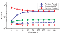
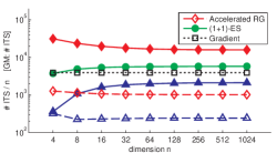
Fig. 1: Average #FES/$n$ (left panel) and #ITS/$n$ (right panel) vs. dimension $n$ on the ellipsoidal function $f_{2}$ to reach a relative accuracy of $1.91\cdot 10^{-6}$ (#ITS for $\mathcal{GM}$). Further data are available in Tables 8 and 9.

We again observe the theoretically expected linear scaling of the number of ITS with dimension for sufficiently large $n$. The mean number of ITS now spans two orders of magnitude for the different algorithms. Standard Random Pursuit outperforms the $\mathcal{RG}$ and the $\mathcal{ES}$ algorithm. Moreover, the accelerated $\mathcal{RP}_{\mu}$ scheme outperforms the $\mathcal{FG}$ scheme by a factor of 4. All methods show, however, an increased overall run time due to the high condition number of the quadratic form. This is also reflected in the increased number of FES that are needed by the line search oracle in the $\mathcal{RP}_{\mu}$ algorithms. The line search oracle now consumes on average 12-14 FES per iteration.

In terms of consumed FES budget we observe that Random Pursuit still outperforms Random Gradient for small dimensions but needs a comparable number of FES for $n\geq 64$ (around 30.000 FES in blocks of $n$). The $\mathcal{ES}$, the $\mathcal{ARP}_{\mu}$, and the $\mathcal{FG}$ algorithm need an order of magnitude fewer FES. The accelerated $\mathcal{RP}_{\mu}$ is only outperformed by the $\mathcal{FG}$ algorithm. The performance of the $\mathcal{ES}$ algorithm is again remarkable given the fact that it does not need information about the parameters $L_{1}$ and $m$ which are of fundamental importance for the accelerated schemes.

6.3.2 Performance on the Full Benchmark Set for $\mathbf{n=64}$

We now illustrate the behavior of the different algorithms on the full benchmark set for fixed dimension $n=64$. We observed similar qualitative behavior for all other dimensions. Table 4 contains the number of ITS needed to reach the scale-dependent accuracy $1.91\cdot 10^{-6}S$ for all algorithms.

	$\mathcal{RP}$			$\mathcal{RG}$			$\mathcal{FG}$			$\mathcal{ARP}$			$\mathcal{ES}$			$\mathcal{GM}$	$\mathcal{GM}_{LS}$
fun.	min	max	mean	min	max	mean	min	max	mean	min	max	mean	min	max	mean	-	-
$f_{1}$	12	14	13	30	34	32	30	34	32	12	14	13	33	41	37	1	1
$f_{2}$	1899	2096	2001	16601	17333	16868	990	1079	1038	233	250	242	5451	5954	5729	3934	3
$f_{3}$	2068	2191	2136	18922	19075	19004	892	970	942	192	678	473	5766	6050	5916	4474	2237
$f_{4}$	954	1023	995	8727	8995	8854	441	534	458	137	188	159	2651	2854	2751	2086	1044
$f_{5}$	26	30	28	-	-	-	-	-	-	26	30	28	73	85	78	-	1

Table 4: Average #ITS/$n$ to reach the relative accuracy $1.91\cdot 10^{-6}$ in dimension $n=64$. For $\mathcal{GM}$ and $\mathcal{GM}_{LS}$ the exact number of ITS is reported. Observed minimum ITS across all (gradient-free) algorithms are marked in bold face for each function.

We observe that Random Pursuit outperforms the $\mathcal{RG}$ and the $\mathcal{ES}$ algorithm, and that the $\mathcal{ARP}_{\mu}$ algorithm outperforms all gradient-free schemes in terms of number of ITS on all functions (with equal performance as Random Pursuit on $f_{1}$ and $f_{5}$). We consistently observe an improved performance of all algorithms on the regularized strongly convex function $f_{4}$ as compared to its convex counterpart $f_{3}$. This expected behavior is most pronounced for the $\mathcal{ARP}_{\mu}$ scheme where, on average, the number of ITS is reduced to $159/473\approx 1/3$.

A comparison between the two gradient schemes reveals that $\mathcal{GM}_{LS}$ outperforms the fixed step size gradient scheme on all test functions. The remarkable performance of $\mathcal{GM}_{LS}$ on $f_{2}$ is due to the fact that the spectrum of the Hessian contains in equal parts two different values (1 and $L$, respectively). A single line search along a gradient direction is thus simultaneously optimal for $n/2$ directions of this function. The $\mathcal{GM}_{LS}$ scheme thus reaches the target accuracy in as few as three steps. This efficiency is lost as soon as the spectrum becomes sufficiently diverse (as indicated by its performance on $f_{4}$). We also remark that the performance of $\mathcal{RP}/\mathcal{GM}_{LS}$ as well as the pair $\mathcal{FG}/\mathcal{GM}$ is in full agreement with theory. We see on functions $f_{3}/f_{4}$ that $\mathcal{RP}$ is about a factor of $n$ slower than the $\mathcal{GM}_{LS}$ due to unavailable gradient information. The same is true for $\mathcal{FG}/\mathcal{GM}$ where $\mathcal{FG}$ is about $4n$ times slower than $\mathcal{GM}$ due to the theoretically needed reduction of the optimal step length by a factor of $1/4$ [29].

For function $f_{4}$ we illustrate the convergence behavior of the different algorithms in Figure 2. After a short algorithm-dependent initial phase we observe linear convergence of all algorithms for fixed dimension, i.e., a constant reduction of the logarithm of the distance to the minimum per iteration.

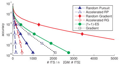
Fig. 2: Average accuracy (in log scale) vs. #ITS/$n$ for all algorithms on $f_{4}$ in dimension $n=64$. Further data are available in [38] in Table S-4.

We also observe that the accelerated Random Pursuit consistently outperforms standard Random Pursuit for all measured accuracies on $f_{4}$ (see Table S-4 in [38] for the corresponding numerical data). This behavior is less pronounced for the function pair $f_{1}/f_{2}$ as shown in Figure 3.

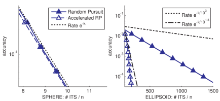
Fig. 3: Numerical convergence rate of standard and accelerated Random Pursuit on $f_{1}$ (left panel) and $f_{2}$ (right panel) in dimension $n=64$. For both instances the theoretically predicted worst-case progress rate (dotted line) is shown for comparison. The rate of the $\mathcal{ARP}$ scheme is compared to the theoretically predicted convergence rate of $\mathcal{FG}$ (slash-dotted line) [29].

On $f_{1}$ both Random Pursuit schemes have identical progress rates that are also consistent with the theoretically predicted one. On $f_{2}$ Random Pursuit outperforms the accelerated scheme for low accuracies (see also Table S-2 in [38] for the numerical data) but is quickly outperformed due to faster progress rate of the accelerated scheme. We also observe that the theoretically predicted worst-case progress rate (dotted line in the right panel of Figure 3) does not reflect the true progress on this test function. Comparison of the numerical results on the function pair $f_{1}/f_{5}$ (see Figure 4) demonstrates the expected invariance under strictly monotone transformations of the Random Pursuit algorithms and the $\mathcal{ES}$ scheme. These algorithms enjoy the same convergence behavior (up to small random variations) to the target solution while the Random Gradient schemes fail to converge to the target accuracy. Note, however, the numbers reported in e.g. Table 4 are not identical for $f_{1}$ and $f_{5}$ because the used stopping criteria are dependent on the scale of the function values. The convergence rates are the same, but more iterations are needed for $f_{5}$ because the required accuracy is considerably smaller.

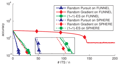
Fig. 4: Numerical convergence rate of the $\mathcal{RP}_{\mu}$, the $\mathcal{ES}$, and the $\mathcal{RG}$ scheme on $f_{1}$ and $f_{5}$ in $n=64$ dimensions. The accuracy is measured in terms of the logarithmic distance to the optimum $\log\left(\left\lVert x_{k}-x^{*}\right\rVert_{2}\right)$.

We also report the performance of the different algorithms in terms of number of FES needed to reach the target accuracy of $1.91\cdot 10^{-6}S$ for the different test functions. For all algorithms the minimum, maximum, and average number of FES are recorded in Table 5.

	$\mathcal{RP}$			$\mathcal{RG}$			$\mathcal{FG}$			$\mathcal{ARP}$			$\mathcal{ES}$
fun.	min	max	mean	min	max	mean	min	max	mean	min	max	mean	min	max	mean
$f_{1}$	47	57	52	60	68	64	57	66	61	50	56	52	33	41	37
$f_{2}$	27723	30272	29071	33202	34667	33736	1980	2159	2077	3035	3247	3159	5451	5954	5729
$f_{3}$	25520	27034	26351	37844	38150	38008	1785	1939	1885	2199	8149	5609	5766	6050	5916
$f_{4}$	11629	12482	12122	17455	17990	17708	883	1069	916	1557	2134	1825	2651	2854	2751
$f_{5}$	338	384	360	-	-	-	-	-	-	342	399	361	73	85	78

Table 5: Average #FES$/n$ to reach the relative accuracy $1.91\cdot 10^{-6}$ in dimension $n=64$. Observed minimum #FES/$n$ across all algorithms are marked in bold face for each function.

We observe that the $\mathcal{RP}_{\mu}$ algorithm outperforms the standard Random Gradient method on all tested functions. However, Random Pursuit is not competitive compared to the accelerated schemes and the $\mathcal{ES}$ algorithm. The accelerated $\mathcal{RP}_{\mu}$ scheme is only outperformed by the $\mathcal{FG}$ algorithm. The latter scheme shows particularly good performance on the convex function $f_{3}$ with considerably lower variance. For functions $f_{2}$–$f_{4}$ the $\mathcal{RP}_{\mu}$ algorithms need around $12-15$ FES per line search oracle call. We emphasize again that the performance of the adaptive step size $\mathcal{ES}$ scheme is remarkable given the fact that it does not need any function-specific parametrization. A comparison to the parameter-free Random Pursuit scheme shows that it needs around four times fewer FES on functions $f_{2}$–$f_{4}$.

We remark that Random Pursuit with discrete sampling, i.e., using the set of signed unit vectors for sample generation (see Section 2.1), yields numerical results on the present benchmark that are consistent with our theoretical predictions. We observed improved performance of Random Pursuit with discrete sampling on the function triplet $f_{1}/f_{2}/f_{5}$. This is evident as the coordinate system of these functions coincide with the standard basis. Thus, algorithms that move along the standard coordinate system are favored. On the function pair $f_{3}/f_{4}$ we do not see any significant deviation from the presented performance results.

param. $\mu$:	1e$-1$	1e$-2$	1e$-3$	1e$-4$	1e$-5$	1e$-6$	1e$-7$	1e$-8$	1e$-9$	1e$-10$
#ITS / n	1986	1982	2013	2017	2001	2001	2001	2001	2020	2020
# FES / n	19824	19781	21435	26120	29071	29495	29537	29542	38993	39070

Table 6: Performance of $\mathcal{RP}_{\mu}$ on the ellipsoid function $f_{2}$, $m=1$, $L=1000$, $S=3200$, $n=64$, for different line search parameters $\mu$. Mean (of 25 repetitions) number of ITS/$n$ and FES/$n$ to reach a relative accuracy of $1.91\cdot 10^{-6}$ are reported.

We also exemplify the influence of the parameter $\mu$ on $\mathcal{RP}_{\mu}$’s performance. We choose the function $f_{2}$ as test instance because the $\mathcal{RP}_{\mu}$ consumes most FES on this function. We vary $\mu$ between $1\textsc{e}$-1 and $1\textsc{e}$-10 and run the $\mathcal{RP}_{\mu}$ scheme 25 times to reach a relative accuracy of $1.91\cdot 10^{-6}$. Mean number of ITS and FES are reported in Table 6. We see that the choice of $\mu$ has almost no influence on the number of ITS to reach the target accuracy, thus justifying the use of ITS as meaningful performance measure. The number of FES span the same order of magnitude ranging from $19824$ for $1\textsc{e}$-1 to $39070$ for $1\textsc{e}$-10. We see that the number of FES for the standard setting $\mu=1\textsc{e}$-5 is approximately in the middle of these extremes (29071 FES). This implies that the qualitative picture of the reported performance comparison is still valid but individual results for $\mathcal{RP}_{\mu}$ and $\mathcal{ARP}_{\mu}$ are improvable by optimally choosing $\mu$. An in-depth analysis of the optimal function-dependent choice of the $\mu$ parameter is subject to future studies.

As a final remark we highlight that the present numerical results for the Random Gradient methods are fully consistent with the ones presented in Nesterov’s paper [29].

7 Discussion and Conclusion

We have derived a convergence proof and convergence rates for Random Pursuit on convex functions. We have used a quadratic upper bound technique to bound the expected single-step progress of the algorithm. Assuming exact line search, this results in global linear convergence for strongly convex functions and convergence of the order $1/k$ for general convex functions.

For line search oracles with relative error $\mu$ the same results have been obtained with convergence rates reduced by a factor of $\frac{1}{1-\mu}$. For inexact line search with absolute error $\mu$, convergence can be established only up to an additive error term depending on $\mu$, the properties of the function and the dimensionality.

The convergence rate of Random Pursuit exceeds the rate of the standard (first-order) Gradient Method by a factor of $n$. Jägersküpper showed that no better performance can be expected for strongly convex functions [15]. He derived a lower bound for algorithms of the form (3) where at each iteration the step size along the random direction is chosen such as to minimize the distance to the minimum $x^{*}$. On sphere functions $f(x)=(x-x^{*})^{T}(x-x^{*})$ Random Pursuit coincides with the described scheme, thus achieving the lower bound.

The numerical experiments showed that (i) standard Random Pursuit is effective on strongly convex functions with moderate condition number, and (ii) the accelerated scheme is comparable to Nesterov’s fast gradient method and outperforms the $\mathcal{ES}$ algorithm. The experimental results also revealed that (i) $\mathcal{RP}_{\mu}$’s empirical convergence is (as predicted by theory) $n$ times slower than the one of the corresponding gradient scheme with line search ($\mathcal{GM}_{LS}$), and (ii) both continuous and discrete sampling can be employed in Random Pursuit. We confirmed the invariance of the $\mathcal{RP}_{\mu}$ algorithms and $\mathcal{ES}$ under monotone transformations of the objective functions on the quasiconvex funnel-shaped function $f_{5}$ where Random Gradient algorithms fail. We also highlighted the remarkable performance of the $\mathcal{ES}$ scheme given the fact that it does not need any function-specific input parameters.

The present theoretical and experimental results hint at a number of potential enhancements for standard Random Pursuit in future work. First, $\mathcal{RP}_{\mu}$’s convergence rate depends on the function-specific parameter $L_{1}$ that bounds the curvature of the objective function. Any reduction of this dependency would imply faster convergence on a larger class of functions. The empirical results on the function pair $f_{1}/f_{2}$ (see Tables S-1 and S-2 in [38]) also suggest that complicated accelerated schemes do not present any significant advantage on functions with small constant $L_{1}$. It is conceivable that Random Pursuit can incorporate a mechanism to learn second-order information about the function “on the fly”, thus improving the conditioning of the original optimization problem and potentially reducing it to the $L_{1}\approx 1$ case. This may be possible using techniques from randomized Quasi-Newton approaches [3, 23, 37] or differential geometry [7]. It is noteworthy that heuristic versions of such an adaptation mechanism have proved extremely useful in practice for adaptive step size algorithms [19, 13, 25]

Second, we have not considered Random Pursuit for constrained optimization problems of the form:

$$\min f(x)\quad\text{subject to}\quad x\in\mathcal{K}\,,$$ (24)

where $\mathcal{K}\subset\mathbb{R}^{n}$ is a convex set. The key challenge is how to treat iterates $x_{k+1}=x_{k}+\texttt{{LSapprox}}(x_{k},u)\cdot u$ generated by the line search oracle that are outside the domain $\mathcal{K}$. A classic idea is to apply a projection operator $\pi_{\mathcal{K}}$ and use the resulting $x^{\prime}_{k+1}:=\pi_{\mathcal{K}}(x_{k+1})$ as the next iterate. However, finding a projection onto a convex set (except for simple bodies such as hyper-parallelepipeds) can be as difficult as the original optimization problem. Moreover, it is an open question whether general convergence can be ensured, and what convergence rates can be achieved. Another possibility is to constrain the line search to the intersection of the line and the convex body $\mathcal{K}$. In this case, it is evident that one can only expect exponentially slow convergence rates for this method. Consider the linear function $f(x)=1^{T}x$ and $\mathcal{K}=\mathbb{R}^{n}_{+}$. Once an iterate $x_{k}$ lies at the boundary $\partial\mathcal{K}$ of the domain, say the first coordinate of $x_{k}$ is zero, then only directions $u$ with positive first coordinate may lead to an improvement. As soon as a constant fraction of the coordinates are zero, the probability of finding an improving direction is exponentially small. Karmanov [17] proposed the following combination of projection and line search constraining: First, a random point $y$ at some fixed distance of the current iterate is drawn uniformly at random and then projected to the set $\mathcal{K}$. A constrained line search is now performed along the line through the current iterate $x_{k}$ and $\pi_{\mathcal{K}}(y)$. It remains open to study the convergence rate of this method.

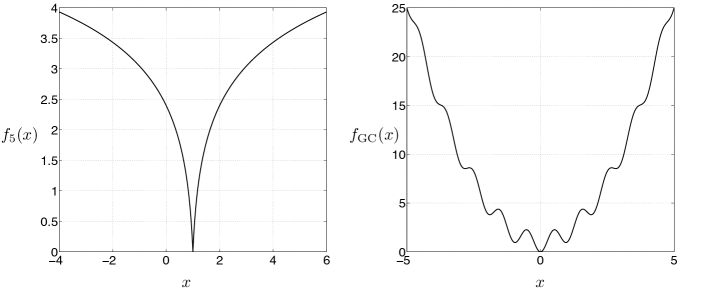
Fig. 5: Left panel: Graph of function $f_{5}$ in 1D. Right Panel: Graph of a globally convex function $f_{\text{GC}}$.

Finally, we envision convergence guarantees and provable convergence rates for Random Pursuit on more general function classes. The invariance of the line search oracle under strictly monotone transformations of the objective function already implied that Random Pursuit converges on certain strictly quasiconvex functions. It also seems in reach to derive convergence guarantees for Random Pursuit on the class of globally convex (or $\delta$-convex) functions [12] or on convex functions with bounded perturbations [30] (see right panel of Figure 5 for the graph of such an instance). This may be achieved by appropriately adapting line search methods to these function classes. In summary, we believe that the theoretical and experimental results on Random Pursuit represent a promising first step toward the design of competitive derivative-free optimization methods that are easy to implement, possess theoretical convergence guarantees, and are useful in practice.

Appendix A Lemma

Lemma 13.

Let $\{f_{t}\}_{t\in\mathbb{N}}$ be a sequence with $f_{i}\in\mathbb{R}_{+}$. Suppose

$$f_{t+1} \leq\left(1-\theta/t\right)f_{t}+C\theta^{2}/t^{2}+D\,,\quad\text{for }t\geq 1,$$

for some constants $\theta>1$, $C>0$ and $D\geq 0$. Then it follows by induction that

$$f_{t}\leq Q(\theta)/t+(t-1)D\,,$$

where $Q(\theta)=\max\left\{\theta^{2}C/(\theta-1),f_{1}\right\}$.

A very similar result was stated without proof in [27] and also Hazan [10] is using the same.

Proof. For $t=1$ it holds that $f_{1}\leq Q(\theta)$ by definition of $Q(\theta)$. Assume that the result holds for $t\geq 1$. If $Q(\theta)=\theta^{2}C/(\theta-1)$ then we deduce:

$$f_{t+1} \leq\frac{\theta^{2}C(t-\theta)}{(\theta-1)t^{2}}+\frac{C\theta^{2}}{t^{2}}+\frac{(t-\theta)(t-1)D}{t}+D$$

$$=\frac{\theta^{2}C(t-1)}{(\theta-1)t^{2}}+\frac{D(t^{2}-\theta(t-1))}{t}\leq\frac{\theta^{2}C}{(\theta-1)(t+1)}+tD\,.$$

If on the other hand $Q(\theta)=f_{1}$, then

$$f_{1}\geq\frac{\theta^{2}C}{(\theta-1)}\quad\Leftrightarrow\quad(\theta-1)f_{1}\geq\theta^{2}C\,,$$

and it follows

$$f_{t+1} \leq\frac{(t-\theta)f_{1}}{t^{2}}+\frac{C\theta^{2}}{t^{2}}+\frac{(t-\theta)(t-1)D}{t}+D$$

$$=\frac{(t-1)f_{1}}{t^{2}}+\frac{\theta^{2}C-(\theta-1)f_{1}}{t^{2}}+\frac{D(t^{2}-\theta(t-1))}{t}\leq\frac{f_{1}}{t+1}+tD\,.\qquad\end@proof$$

Appendix B Tables

B.1 Initial $\sigma_{0}$ of the $\mathcal{ES}$ algorithm for all test functions

Table 7 reports the empirically determined optimal initial step sizes $\sigma_{0}$ used as input to the $\mathcal{ES}$ algorithm.

dim	$f_{1}$	$f_{2}$	$f_{3}$	$f_{4}$
4	0.79158	1.3897	0.2054	0.20395
8	0.49167	0.78761	0.08922	0.088145
16	0.32692	0.49500	0.04134	0.041273
32	0.22292	0.32547	0.019911	0.019905
64	0.15542	0.22243	0.0097212	0.0097127
128	0.10925	0.15638	0.0048305	0.0048335
256	0.076658	0.10902	0.0024171	0.0024114
512	0.054339	0.076568	0.0012012	0.0012006
1024	0.038367	0.054173	0.00060284	0.00060223

Table 7: The initial values of the stepsize $\sigma$ for $(1+1)$-ES on the test functions for various dimensions.

B.2 Data for the ellipsoid test function for $\mathbf{n\leq 1024}$

Tables 8 and 9 report the numerical data used to produce Figure 1.

	$\mathcal{RP}$			$\mathcal{RG}$			$\mathcal{FG}$			$\mathcal{ARP}$			$\mathcal{ES}$			$\mathcal{GM}$	$\mathcal{GM}_{LS}$
n	min	max	mean	min	max	mean	min	max	mean	min	max	mean	min	max	mean	-	-
4	236	472	364	28322	33608	31549	966	1575	1282	124	682	322	2491	4557	3784	3934	3
8	787	1241	1088	22461	24610	23666	981	1262	1155	174	285	226	3786	5799	4906	3934	3
16	1326	1763	1624	18981	20403	19805	975	1164	1076	218	256	232	4967	6034	5400	3934	3
32	1769	2026	1880	17381	18393	17858	968	1102	1048	221	256	237	5183	6145	5625	3934	3
64	1899	2096	2001	16601	17333	16868	990	1079	1038	233	250	242	5451	5954	5729	3934	3
128	1987	2145	2076	16183	16721	16376	978	1061	1030	237	252	245	5512	5964	5753	3934	3
256	2063	2173	2117	15960	16276	16115	1007	1053	1026	238	251	245	5603	6065	5805	3934	3
512	2081	2159	2119	15937	16103	16011	1015	1037	1026	239	249	244	5706	5909	5818	3934	3
1024	2109	2152	2132	15846	16065	15955	1020	1035	1027	242	247	244	5759	5932	5833	3934	3

Table 8: Ellipsoid function $f_{2}$ to accuracy $1.91\cdot 10^{-6}$, $S=50n$, $L=1000$. #ITS$/n$, ($\mathcal{GM}$ and $\mathcal{GM}_{LS}$: #ITS).

	$\mathcal{RP}$			$\mathcal{RG}$			$\mathcal{FG}$			$\mathcal{ARP}$			$\mathcal{ES}$
n	min	max	mean	min	max	mean	min	max	mean	min	max	mean	min	max	mean
4	3155	6236	4775	56643	67217	63097	1933	3150	2564	1408	6983	3631	2491	4557	3784
8	11043	17124	15216	44923	49221	47331	1963	2525	2310	2113	3483	2774	3786	5799	4906
16	19182	25225	23320	37962	40806	39610	1951	2329	2152	2730	3239	2930	4967	6034	5400
32	25768	29258	27302	34762	36785	35715	1937	2203	2097	2870	3243	3043	5183	6145	5625
64	27723	30272	29071	33202	34667	33736	1980	2159	2077	3035	3247	3159	5451	5954	5729
128	28791	30757	29894	32365	33441	32753	1956	2121	2059	3139	3354	3259	5512	5964	5753
256	29363	30691	30016	31920	32552	32230	2013	2106	2053	3210	3411	3322	5603	6065	5805
512	29173	30167	29644	31874	32207	32022	2031	2075	2053	3311	3453	3386	5706	5909	5818
1024	29316	29914	29639	31692	32131	31910	2041	2069	2054	3455	3541	3494	5759	5932	5833

Table 9: Ellipsoid function $f_{2}$ to accuracy $1.91\cdot 10^{-6}$, $S=50n$, $L=1000$. #FES$/n$.

Supporting Online Material for
OPTIMIZATION OF CONVEX FUNCTIONS WITH RANDOM PURSUIT^∗

S. U. Stich^†, C. L. Müller^‡, and B. Gärtner^§

Appendix C Exemplary Matlab Codes

C.1 Accelerated Random Pursuit

⬇

ction[fval,x,funeval]=rp_acc(fitfun,xstart,N,mu,m,L)

%AlgorithmAcceleratedRandomPursuit

%fitfunnameorfunctionhandle

%Nnumberofiterations

%mulinesearchaccuracyfuneval#functionevaluations

%m,Lparametersforquadraticupperandlowerbounds

%linesearchparameters

opts=optimset('Display',’off’,'LargeScale',’off’,'TolX',mu); funeval=0; x=xstart; n=length(xstart); th=1/(L*n^2); ga=m; v=x; fori=1:N

p=[1/th,ga-m,-ga];be=max(roots(p));

de=(be*ga)/(ga+be*m);y=(1-de)*x+de*v;

ga=(1-be)*ga+be*m;la=be/ga*m;

d=randn(size(xstart));d=d/norm(d);

[sigma,fval, ,infos]=...

fminunc(@(sigma)feval(fitfun,y+sigma*d),0,opts);funeval=funeval+infos.funcCount;

x=y+sigma*d;v=(1-la)*v+la*y+sigma/(be*n)*d;

end

Fig. S-6: Matlab code for algorithm $\mathcal{ARP}_{\mu}$

C.2 Random Pursuit

⬇

ction[fval,x,funeval]=rp(fitfun,xstart,N,mu)

%AlgorithmRandomPursuit fitfunnameorfunctionhandleNnumberofiterationsmulinesearchaccuracy

%funeval#functionevaluations searchparameters opts=optimset(’Display’,'off',’LargeScale’,'off',’TolX’,mu);

funeval=0;

x=xstart;

fori=1:Nd=randn(size(xstart));d=d/norm(d);[sigma,fval, ,infos]=...

fminunc(@(sigma)feval(fitfun,x+sigma*d),0,opts);funeval=funeval+infos.funcCount;x=x+sigma*d;

end

Fig. S-7: Matlab code for algorithm $\mathcal{RP}_{\mu}$

C.3 Random Gradient

⬇

ction[fval,x]=rg(fitfun,xstart,N,eps,L)

%RandomGradient[Nesterov2011]

%fitfunnameorfunctionhandle

%Nnumberofiterations

%epsfinitedifferenceparameter

%Lquadraticupperbound

x=xstart;

n=length(xstart);

h=1/(4*L*(n+4)); fori=1:N

d=randn(size(xstart));

g=(feval(fitfun,x+eps*d)-feval(fitfun,x))/eps;x=x-h*g*d; end fval=feval(fitfun,x);

Fig. S-8: Matlab code for algorithm $\mathcal{RG}$

C.4 Accelerated Random Gradient

⬇

ction[fval,x]=rg_acc(fitfun,xstart,N,eps,m,L)AcceleratedRandomGradient[Nesterov2011]

%fitfunnameorfunctionhandle

%Nnumberofiterations

%epsfinitedifferenceparameter

%m,Lparametersforquadraticupperandlowerbounds

x=xstart;

n=length(xstart);

h=1/(4*L*(n+4)); th=1/(16*L*(n+1)^2); ga=m; v=x; fori=1:N

p=[1/th,ga-m,-ga];be=max(roots(p));

de=(be*ga)/(ga+be*m);y=(1-de)*x+de*v;

ga=(1-be)*ga+be*m;la=be/ga*m;

d=randn(size(xstart));g=(feval(fitfun,x+eps*d)-feval(fitfun,x))/eps;

x=y-h*g*d;v=(1-la)*v+la*y-th/be*g*d;

end

fval=feval(fitfun,x);

Fig. S-9: Matlab code for algorithm $\mathcal{FG}$

C.5 (1+1)-ES

⬇

ction[fval,x]=es(fitfun,xstart,N,sigma)(1+1)-ES

%fitfunnameorfunctionhandle

%Nnumberofiterations

%sigmainitialstepsizefuneval#functionevaluations

fval=feval(fitfun,xstart); x=xstart; ss=exp(1/3); ff=exp(1/3*(-0.27)/(1-0.27)); fori=1:N

d=randn(size(xstart));

f=feval(fitfun,x+sigma*d);

iff$\leq$fvalx=x+sigma*d;fval=f;sigma=sigma*ss;

elsesigma=sigma*ff;

end

end

Fig. S-10: Matlab code for algorithm $\mathcal{ES}$

Appendix D Tables

D.1 Number of iterations for increasing accuracy for $\mathbf{n=64}$

Tables S-10 - S-14 summarize the number of iterations needed to achieve a corresponding relative accuracy (acc) for fixed dimension $n=64$.

	$\mathcal{RP}$			$\mathcal{RG}$			$\mathcal{FG}$			$\mathcal{ARP}$			$\mathcal{ES}$			$\mathcal{GM}$	$\mathcal{GM}_{LS}$
acc.	min	max	mean	min	max	mean	min	max	mean	min	max	mean	min	max	mean	-	-
$6.25\cdot 10^{-2}$	2	3	3	6	8	7	6	8	7	2	3	3	6	9	8	1	1
$3.12\cdot 10^{-2}$	3	4	3	8	10	8	8	10	8	3	4	3	8	12	10	1	1
$1.56\cdot 10^{-2}$	4	5	4	9	12	10	9	12	10	4	5	4	10	14	12	1	1
$7.81\cdot 10^{-3}$	4	6	5	11	13	12	11	13	12	4	5	5	12	16	14	1	1
$3.91\cdot 10^{-3}$	5	6	5	13	15	14	13	15	14	5	6	5	14	18	16	1	1
$1.95\cdot 10^{-3}$	5	7	6	14	17	15	14	17	15	5	7	6	15	20	18	1	1
$9.77\cdot 10^{-4}$	6	8	7	16	18	17	16	18	17	6	8	7	17	22	20	1	1
$4.88\cdot 10^{-4}$	7	9	7	18	20	19	18	20	19	7	9	7	18	24	21	1	1
$2.44\cdot 10^{-4}$	7	9	8	19	22	20	19	22	20	7	9	8	20	26	23	1	1
$1.22\cdot 10^{-4}$	8	10	9	21	24	22	21	24	22	8	10	9	22	28	25	1	1
$6.10\cdot 10^{-5}$	9	10	10	22	26	24	22	26	24	9	11	9	23	31	27	1	1
$3.05\cdot 10^{-5}$	9	11	10	24	28	25	24	28	25	10	11	10	26	32	29	1	1
$1.53\cdot 10^{-5}$	10	12	11	25	29	27	25	29	27	10	12	11	28	35	31	1	1
$7.63\cdot 10^{-6}$	11	13	12	27	31	29	27	31	29	11	13	12	29	36	33	1	1
$3.81\cdot 10^{-6}$	11	13	12	28	32	30	28	32	30	12	13	12	31	38	35	1	1
$1.91\cdot 10^{-6}$	12	14	13	30	34	32	30	34	32	12	14	13	33	41	37	1	1

Table S-10: Sphere function $f_{1}$, $m=1$, $L=1$, $S=32$, $n=64$. #ITS$/n$, ($\mathcal{GM}$, $\mathcal{GM}_{LS}$: #ITS).

	$\mathcal{RP}$			$\mathcal{RG}$			$\mathcal{FG}$			$\mathcal{ARP}$			$\mathcal{ES}$			$\mathcal{GM}$	$\mathcal{GM}_{LS}$
acc.	min	max	mean	min	max	mean	min	max	mean	min	max	mean	min	max	mean	-	-
$6.25\cdot 10^{-2}$	2	3	2	9	11	10	5	18	16	64	79	71	5	9	6	1	1
$3.12\cdot 10^{-2}$	2	3	3	11	13	12	17	21	18	70	86	77	6	10	8	1	1
$1.56\cdot 10^{-2}$	3	4	3	13	15	14	31	359	261	77	93	84	7	19	10	1	1
$7.81\cdot 10^{-3}$	4	132	53	15	20	17	340	423	380	84	101	91	18	465	268	1	1
$3.91\cdot 10^{-3}$	104	298	210	381	1103	677	404	484	444	92	125	107	481	928	723	124	2
$1.95\cdot 10^{-3}$	273	460	373	1863	2578	2150	464	544	504	101	140	129	936	1410	1177	470	2
$9.77\cdot 10^{-4}$	433	624	536	3340	4062	3624	521	601	562	129	153	143	1376	1869	1631	817	2
$4.88\cdot 10^{-4}$	598	787	700	4815	5536	5094	576	657	618	142	164	153	1826	2325	2085	1163	2
$2.44\cdot 10^{-4}$	761	954	862	6280	7018	6564	630	712	673	153	174	162	2264	2774	2538	1509	2
$1.22\cdot 10^{-4}$	921	1118	1024	7754	8488	8036	683	767	727	161	183	170	2732	3239	2994	1856	2
$6.10\cdot 10^{-5}$	1080	1284	1187	9232	9961	9508	736	820	781	168	191	178	3172	3690	3447	2202	2
$3.05\cdot 10^{-5}$	1243	1446	1350	10712	11439	10980	787	873	833	176	199	187	3635	4138	3905	2549	3
$1.53\cdot 10^{-5}$	1406	1607	1512	12179	12906	12453	839	925	885	189	214	201	4083	4593	4361	2895	3
$7.63\cdot 10^{-6}$	1570	1766	1675	13654	14388	13923	890	977	936	203	227	217	4537	5042	4819	3241	3
$3.81\cdot 10^{-6}$	1732	1928	1837	15130	15854	15395	940	1029	988	219	238	230	4989	5492	5273	3588	3
$1.91\cdot 10^{-6}$	1899	2096	2001	16601	17333	16868	990	1079	1038	233	250	242	5451	5954	5729	3934	3

Table S-11: Ellipsoid function $f_{2}$, $m=1$, $L=1000$, $S=3200$, $n=64$. #ITS$/n$, ($\mathcal{GM}$, $\mathcal{GM}_{LS}$: #ITS).

	$\mathcal{RP}$			$\mathcal{RG}$			$\mathcal{FG}$			$\mathcal{ARP}$			$\mathcal{ES}$			$\mathcal{GM}$	$\mathcal{GM}_{LS}$
acc.	min	max	mean	min	max	mean	min	max	mean	min	max	mean	min	max	mean	-	-
$6.25\cdot 10^{-2}$	0	0	0	0	0	0	0	0	0	0	0	0	0	0	0	1	1
$3.12\cdot 10^{-2}$	0	0	0	0	0	0	0	0	0	0	0	0	0	0	0	1	1
$1.56\cdot 10^{-2}$	0	0	0	0	0	0	0	0	0	0	0	0	0	0	0	1	1
$7.81\cdot 10^{-3}$	1	1	1	3	5	4	2	4	3	0	1	1	2	4	3	1	1
$3.91\cdot 10^{-3}$	3	4	3	18	23	21	8	13	10	3	19	8	6	10	9	5	3
$1.95\cdot 10^{-3}$	8	12	10	74	84	79	29	40	34	12	66	25	22	31	26	19	10
$9.77\cdot 10^{-4}$	26	37	31	256	283	269	55	84	70	22	75	41	73	102	86	64	32
$4.88\cdot 10^{-4}$	79	109	92	790	837	811	104	152	130	33	132	61	233	292	257	191	96
$2.44\cdot 10^{-4}$	200	264	228	1993	2065	2022	164	258	201	35	173	87	577	700	633	477	239
$1.22\cdot 10^{-4}$	405	501	453	3955	4053	4004	224	328	279	58	199	127	1142	1344	1249	945	473
$6.10\cdot 10^{-5}$	665	778	723	6349	6465	6412	293	382	348	74	255	151	1867	2101	1998	1512	756
$3.05\cdot 10^{-5}$	948	1060	1005	8849	8964	8917	369	427	402	88	391	213	2641	2891	2780	2101	1051
$1.53\cdot 10^{-5}$	1229	1345	1288	11375	11482	11435	397	613	442	96	449	265	3406	3692	3563	2694	1347
$7.63\cdot 10^{-6}$	1509	1619	1570	13886	14016	13958	450	894	677	129	533	342	4223	4461	4348	3288	1644
$3.81\cdot 10^{-6}$	1792	1902	1853	16401	16545	16482	463	935	887	188	632	400	5008	5254	5133	3881	1940
$1.91\cdot 10^{-6}$	2068	2191	2136	18922	19075	19004	892	970	942	192	678	473	5766	6050	5916	4474	2237

Table S-12: Nesterov smooth $f_{3}$, $L=1000$, $S=10833$, $n=64$. #ITS$/n$, ($\mathcal{GM}$, $\mathcal{GM}_{LS}$: #ITS).

	$\mathcal{RP}$			$\mathcal{RG}$			$\mathcal{FG}$			$\mathcal{ARP}$			$\mathcal{ES}$			$\mathcal{GM}$	$\mathcal{GM}_{LS}$
acc.	min	max	mean	min	max	mean	min	max	mean	min	max	mean	min	max	mean	-	-
$6.25\cdot 10^{-2}$	1	2	1	7	9	8	4	5	5	1	6	2	3	5	4	2	1
$3.12\cdot 10^{-2}$	3	5	4	25	31	28	10	16	13	5	19	11	8	13	11	7	4
$1.56\cdot 10^{-2}$	8	12	10	79	90	82	27	37	33	9	45	22	19	35	27	19	10
$7.81\cdot 10^{-3}$	19	31	24	199	219	204	46	70	59	21	53	32	52	76	65	48	24
$3.91\cdot 10^{-3}$	43	62	50	415	458	432	74	107	88	25	58	41	109	152	135	102	51
$1.95\cdot 10^{-3}$	82	106	90	772	824	791	104	140	118	39	88	53	214	272	247	187	94
$9.77\cdot 10^{-4}$	131	166	146	1248	1341	1284	138	177	157	49	96	65	352	447	399	303	152
$4.88\cdot 10^{-4}$	195	236	214	1841	1965	1900	169	216	191	52	109	73	533	638	587	449	225
$2.44\cdot 10^{-4}$	267	317	295	2540	2694	2621	195	259	228	64	114	82	740	875	810	619	310
$1.22\cdot 10^{-4}$	352	409	384	3326	3513	3420	244	293	266	68	127	95	976	1132	1059	807	404
$6.10\cdot 10^{-5}$	441	506	479	4174	4387	4277	282	335	306	89	132	107	1233	1403	1325	1009	505
$3.05\cdot 10^{-5}$	539	605	579	5057	5288	5168	321	376	342	96	160	119	1508	1681	1603	1219	610
$1.53\cdot 10^{-5}$	642	715	682	5969	6206	6079	351	402	376	108	168	130	1788	1974	1885	1434	717
$7.63\cdot 10^{-6}$	740	816	786	6893	7138	7001	383	430	409	117	177	138	2071	2269	2173	1650	826
$3.81\cdot 10^{-6}$	845	920	890	7816	8064	7926	423	453	435	127	184	148	2357	2568	2462	1868	935
$1.91\cdot 10^{-6}$	954	1023	995	8727	8995	8854	441	534	458	137	188	159	2651	2854	2751	2086	1044

Table S-13: Nesterov strongly convex function $f_{4}$, $m=1$, $L=1000$, $S=1000$, $n=64$. #ITS$/n$, ($\mathcal{GM}$, $\mathcal{GM}_{LS}$: #ITS),

	$\mathcal{RP}$			$\mathcal{RG}$			$\mathcal{FG}$			$\mathcal{ARP}$			$\mathcal{ES}$			$\mathcal{GM}$	$\mathcal{GM}_{LS}$
acc.	min	max	mean	min	max	mean	min	max	mean	min	max	mean	min	max	mean	-	-
$6.25\cdot 10^{-2}$	4	6	5	-	-	-	-	-	-	4	6	5	13	17	14	-	1
$3.12\cdot 10^{-2}$	7	9	7	-	-	-	-	-	-	7	8	7	19	25	22	-	1
$1.56\cdot 10^{-2}$	8	11	9	-	-	-	-	-	-	8	10	9	24	32	27	-	1
$7.81\cdot 10^{-3}$	10	13	11	-	-	-	-	-	-	10	12	11	29	37	32	-	1
$3.91\cdot 10^{-3}$	11	15	12	-	-	-	-	-	-	12	14	12	32	42	36	-	1
$1.95\cdot 10^{-3}$	13	16	14	-	-	-	-	-	-	13	15	14	35	46	40	-	1
$9.77\cdot 10^{-4}$	14	17	15	-	-	-	-	-	-	14	17	15	39	50	43	-	1
$4.88\cdot 10^{-4}$	16	19	17	-	-	-	-	-	-	15	18	17	43	54	47	-	1
$2.44\cdot 10^{-4}$	17	20	18	-	-	-	-	-	-	17	20	18	47	58	51	-	1
$1.22\cdot 10^{-4}$	18	22	19	-	-	-	-	-	-	18	22	19	51	62	55	-	1
$6.10\cdot 10^{-5}$	19	23	21	-	-	-	-	-	-	19	23	21	55	66	59	-	1
$3.05\cdot 10^{-5}$	21	24	22	-	-	-	-	-	-	21	25	22	59	70	63	-	1
$1.53\cdot 10^{-5}$	22	25	23	-	-	-	-	-	-	22	26	23	62	74	67	-	1
$7.63\cdot 10^{-6}$	23	27	25	-	-	-	-	-	-	23	28	25	67	77	70	-	1
$3.81\cdot 10^{-6}$	25	28	26	-	-	-	-	-	-	24	29	26	71	81	74	-	1
$1.91\cdot 10^{-6}$	26	30	28	-	-	-	-	-	-	26	30	28	73	85	78	-	1

Table S-14: Funnel function $f_{5}$, $S=32$, $n=64$. #ITS$/n$, ($\mathcal{GM}$, $\mathcal{GM}_{LS}$: #ITS).

D.2 Number of function evaluations for increasing accuracy for fixed dimension $n=64$

Tables S-15 - S-19 summarize the number of function evaluations needed to achieve a corresponding relative accuracy (acc) for fixed dimension $n=64$.

	$\mathcal{RP}$			$\mathcal{RG}$			$\mathcal{FG}$			$\mathcal{ARP}$			$\mathcal{ES}$
acc.	min	max	mean	min	max	mean	min	max	mean	min	max	mean	min	max	mean
$6.25\cdot 10^{-2}$	10	14	12	11	15	14	12	15	13	9	13	11	6	9	8
$3.12\cdot 10^{-2}$	12	17	14	15	19	17	15	18	17	12	16	14	8	12	10
$1.56\cdot 10^{-2}$	15	20	17	18	23	20	18	21	20	15	19	17	10	14	12
$7.81\cdot 10^{-3}$	17	23	20	22	27	24	21	25	23	17	22	20	12	16	14
$3.91\cdot 10^{-3}$	20	27	22	25	30	27	24	28	26	20	25	22	14	18	16
$1.95\cdot 10^{-3}$	22	29	25	28	34	30	27	32	29	22	29	25	15	20	18
$9.77\cdot 10^{-4}$	25	33	28	32	37	34	29	35	33	24	32	27	17	22	20
$4.88\cdot 10^{-4}$	27	35	31	35	40	37	32	38	36	27	35	30	18	24	21
$2.44\cdot 10^{-4}$	30	38	33	38	44	41	35	42	39	29	38	33	20	26	23
$1.22\cdot 10^{-4}$	32	40	36	41	47	44	38	45	42	32	40	36	22	28	25
$6.10\cdot 10^{-5}$	35	42	39	44	52	47	41	48	45	36	43	38	23	31	27
$3.05\cdot 10^{-5}$	38	44	42	47	56	51	44	51	49	39	46	41	26	32	29
$1.53\cdot 10^{-5}$	41	48	44	51	58	54	47	55	52	41	49	44	28	35	31
$7.63\cdot 10^{-6}$	43	52	47	53	61	57	51	58	55	44	51	47	29	36	33
$3.81\cdot 10^{-6}$	45	54	50	57	65	60	54	63	58	47	53	49	31	38	35
$1.91\cdot 10^{-6}$	47	57	52	60	68	64	57	66	61	50	56	52	33	41	37

Table S-15: Sphere function $f_{1}$, $m=1$, $L=1$, $S=32$, $n=64$. #FES$/n$.

	$\mathcal{RP}$			$\mathcal{RG}$			$\mathcal{FG}$			$\mathcal{ARP}$			$\mathcal{ES}$
acc.	min	max	mean	min	max	mean	min	max	mean	min	max	mean	min	max	mean
$6.25\cdot 10^{-2}$	12	21	16	18	22	20	10	36	33	637	809	733	5	9	6
$3.12\cdot 10^{-2}$	15	25	19	21	25	23	34	41	37	705	883	802	6	10	8
$1.56\cdot 10^{-2}$	20	32	25	25	30	28	62	717	522	777	966	872	7	19	10
$7.81\cdot 10^{-3}$	29	1671	662	30	39	34	680	847	760	863	1092	963	18	465	268
$3.91\cdot 10^{-3}$	1416	3925	2803	761	2206	1354	808	968	887	978	1418	1185	481	928	723
$1.95\cdot 10^{-3}$	3809	6240	5125	3725	5155	4300	928	1087	1008	1054	1613	1489	936	1410	1177
$9.77\cdot 10^{-4}$	6096	8577	7458	6681	8124	7248	1042	1203	1124	1526	1790	1688	1376	1869	1631
$4.88\cdot 10^{-4}$	8495	10961	9848	9629	11072	10189	1152	1315	1236	1702	1955	1835	1826	2325	2085
$2.44\cdot 10^{-4}$	10936	13455	12278	12560	14036	13129	1259	1425	1347	1844	2108	1966	2264	2774	2538
$1.22\cdot 10^{-4}$	13340	15896	14705	15507	16977	16072	1365	1533	1455	1960	2242	2088	2732	3239	2994
$6.10\cdot 10^{-5}$	15726	18390	17144	18463	19921	19015	1471	1641	1562	2068	2362	2211	3172	3690	3447
$3.05\cdot 10^{-5}$	18147	20800	19566	21423	22877	21960	1575	1747	1666	2188	2508	2353	3635	4138	3905
$1.53\cdot 10^{-5}$	20573	23183	21970	24357	25812	24906	1678	1851	1770	2389	2743	2552	4083	4593	4361
$7.63\cdot 10^{-6}$	22981	25521	24375	27308	28776	27846	1780	1954	1873	2627	2918	2789	4537	5042	4819
$3.81\cdot 10^{-6}$	25337	27890	26733	30259	31707	30790	1880	2057	1975	2857	3083	2993	4989	5492	5273
$1.91\cdot 10^{-6}$	27723	30272	29071	33202	34667	33736	1980	2159	2077	3035	3247	3159	5451	5954	5729

Table S-16: Ellipsoid function $f_{2}$, $m=1$, $L=1000$, $S=3200$, $n=64$. #FES/$n$.

	$\mathcal{RP}$			$\mathcal{RG}$			$\mathcal{FG}$			$\mathcal{ARP}$			$\mathcal{ES}$
acc.	min	max	mean	min	max	mean	min	max	mean	min	max	mean	min	max	mean
$6.25\cdot 10^{-2}$	0	0	0	0	0	0	0	0	0	0	0	0	0	0	0
$3.12\cdot 10^{-2}$	0	0	0	0	0	0	0	0	0	0	0	0	0	0	0
$1.56\cdot 10^{-2}$	0	0	0	0	0	0	0	0	0	0	0	0	0	0	0
$7.81\cdot 10^{-3}$	5	8	7	7	10	8	5	7	6	4	12	7	2	4	3
$3.91\cdot 10^{-3}$	22	33	27	36	45	42	17	25	21	29	163	66	6	10	9
$1.95\cdot 10^{-3}$	73	123	96	147	169	158	58	80	67	102	604	221	22	31	26
$9.77\cdot 10^{-4}$	282	410	344	511	566	538	110	167	140	198	690	375	73	102	86
$4.88\cdot 10^{-4}$	930	1304	1094	1579	1675	1621	208	305	261	301	1264	584	233	292	257
$2.44\cdot 10^{-4}$	2440	3232	2788	3987	4130	4045	327	517	401	328	1716	866	577	700	633
$1.22\cdot 10^{-4}$	4996	6186	5588	7909	8106	8009	448	656	557	574	2132	1332	1142	1344	1249
$6.10\cdot 10^{-5}$	8225	9610	8942	12697	12930	12824	586	765	696	763	2864	1621	1867	2101	1998
$3.05\cdot 10^{-5}$	11739	13117	12445	17699	17928	17833	739	855	803	903	4485	2372	2641	2891	2780
$1.53\cdot 10^{-5}$	15220	16645	15948	22750	22963	22870	795	1225	885	1004	5201	3010	3406	3692	3563
$7.63\cdot 10^{-6}$	18678	20032	19423	27772	28033	27917	900	1788	1355	1410	6242	3979	4223	4461	4348
$3.81\cdot 10^{-6}$	22154	23511	22902	32801	33091	32963	926	1870	1775	2145	7381	4691	5008	5254	5133
$1.91\cdot 10^{-6}$	25520	27034	26351	37844	38150	38008	1785	1939	1885	2199	8149	5609	5766	6050	5916

Table S-17: Nesterov smooth $f_{3}$, $L=1000$, $S=10833$, $n=64$. #FES$/n$.

	$\mathcal{RP}$			$\mathcal{RG}$			$\mathcal{FG}$			$\mathcal{ARP}$			$\mathcal{ES}$
acc.	min	max	mean	min	max	mean	min	max	mean	min	max	mean	min	max	mean
$6.25\cdot 10^{-2}$	8	15	12	13	18	15	8	11	9	8	52	15	3	5	4
$3.12\cdot 10^{-2}$	29	45	35	50	61	56	21	32	26	43	173	93	8	13	11
$1.56\cdot 10^{-2}$	74	120	97	157	179	164	54	75	66	83	421	193	19	35	27
$7.81\cdot 10^{-3}$	198	342	255	397	438	408	93	139	119	184	497	290	52	76	65
$3.91\cdot 10^{-3}$	490	718	570	831	915	864	148	214	175	223	555	391	109	152	135
$1.95\cdot 10^{-3}$	969	1258	1071	1543	1648	1583	208	281	237	373	896	516	214	272	247
$9.77\cdot 10^{-4}$	1578	2012	1757	2495	2682	2568	276	354	314	477	989	662	352	447	399
$4.88\cdot 10^{-4}$	2374	2877	2605	3681	3929	3800	338	433	383	530	1144	763	533	638	587
$2.44\cdot 10^{-4}$	3260	3883	3607	5079	5387	5242	389	519	457	675	1209	876	740	875	810
$1.22\cdot 10^{-4}$	4315	5011	4710	6653	7026	6840	487	587	532	727	1370	1037	976	1132	1059
$6.10\cdot 10^{-5}$	5417	6220	5882	8347	8774	8555	563	671	612	978	1437	1179	1233	1403	1325
$3.05\cdot 10^{-5}$	6621	7435	7116	10113	10577	10337	642	752	685	1074	1782	1323	1508	1681	1603
$1.53\cdot 10^{-5}$	7872	8772	8371	11937	12411	12159	702	804	753	1212	1882	1468	1788	1974	1885
$7.63\cdot 10^{-6}$	9069	10005	9628	13786	14275	14002	766	861	818	1286	1986	1559	2071	2269	2173
$3.81\cdot 10^{-6}$	10331	11264	10885	15633	16129	15852	845	906	870	1448	2078	1687	2357	2568	2462
$1.91\cdot 10^{-6}$	11629	12482	12122	17455	17990	17708	883	1069	916	1557	2134	1825	2651	2854	2751

Table S-18: Nesterov strongly convex function $f_{4}$, $m=1$, $L=1000$, $S=1000$ $n=64$. #FES$/n$.

	$\mathcal{RP}$			$\mathcal{RG}$			$\mathcal{FG}$			$\mathcal{ARP}$			$\mathcal{ES}$
acc.	min	max	mean	min	max	mean	min	max	mean	min	max	mean	min	max	mean
$6.25\cdot 10^{-2}$	37	58	45	-	-	-	-	-	-	40	51	46	13	17	14
$3.12\cdot 10^{-2}$	63	86	71	-	-	-	-	-	-	62	76	70	19	25	22
$1.56\cdot 10^{-2}$	83	110	92	-	-	-	-	-	-	84	102	92	24	32	27
$7.81\cdot 10^{-3}$	103	129	112	-	-	-	-	-	-	103	123	112	29	37	32
$3.91\cdot 10^{-3}$	118	150	132	-	-	-	-	-	-	123	144	132	32	42	36
$1.95\cdot 10^{-3}$	140	168	151	-	-	-	-	-	-	140	167	151	35	46	40
$9.77\cdot 10^{-4}$	159	187	171	-	-	-	-	-	-	159	191	171	39	50	43
$4.88\cdot 10^{-4}$	178	207	190	-	-	-	-	-	-	177	212	192	43	54	47
$2.44\cdot 10^{-4}$	196	230	210	-	-	-	-	-	-	197	231	211	47	58	51
$1.22\cdot 10^{-4}$	215	252	232	-	-	-	-	-	-	218	265	234	51	62	55
$6.10\cdot 10^{-5}$	236	270	252	-	-	-	-	-	-	239	289	255	55	66	59
$3.05\cdot 10^{-5}$	257	293	273	-	-	-	-	-	-	257	313	275	59	70	63
$1.53\cdot 10^{-5}$	279	316	294	-	-	-	-	-	-	277	330	295	62	74	67
$7.63\cdot 10^{-6}$	297	340	316	-	-	-	-	-	-	295	355	317	67	77	70
$3.81\cdot 10^{-6}$	320	365	339	-	-	-	-	-	-	318	378	338	71	81	74
$1.91\cdot 10^{-6}$	338	384	360	-	-	-	-	-	-	342	399	361	73	85	78

Table S-19: Funnel function $f_{5}$, $S=32$ $n=64$. #FES$/n$.

D.3 Different line search parameters for fixed dimension $n=64$

Tables S-20 and S-21 summarize the number of function evaluations needed by $\mathcal{RP}_{\mu}$ on the ellipsoid function $f_{2}$ to achieve a relative accuracy of $1.91\cdot 10^{-6}$ for different parameters $\mu$ that were passed to the used Matlab line search (cf. Figure S-7).

acc.	1e$-1$	1e$-2$	1e$-3$	1e$-4$	1e$-5$	1e$-6$	1e$-7$	1e$-8$	1e$-9$	1e$-10$
$6.25\cdot 10^{-2}$	2	2	2	2	2	2	2	2	2	2
$3.12\cdot 10^{-2}$	3	3	3	3	3	3	3	3	3	3
$1.56\cdot 10^{-2}$	3	3	3	3	3	3	3	3	3	3
$7.81\cdot 10^{-3}$	57	50	56	65	53	53	53	53	73	73
$3.91\cdot 10^{-3}$	201	194	219	225	210	210	210	210	232	232
$1.95\cdot 10^{-3}$	360	353	382	389	373	373	373	373	395	395
$9.77\cdot 10^{-4}$	523	516	546	552	536	536	536	536	558	558
$4.88\cdot 10^{-4}$	685	678	709	715	700	700	700	700	721	721
$2.44\cdot 10^{-4}$	849	842	871	878	862	862	862	862	883	883
$1.22\cdot 10^{-4}$	1011	1004	1035	1041	1024	1024	1024	1024	1045	1045
$6.10\cdot 10^{-5}$	1173	1166	1198	1203	1187	1187	1187	1187	1208	1208
$3.05\cdot 10^{-5}$	1335	1330	1360	1366	1350	1350	1350	1350	1370	1370
$1.53\cdot 10^{-5}$	1497	1494	1523	1528	1512	1512	1512	1512	1533	1533
$7.63\cdot 10^{-6}$	1661	1657	1686	1691	1675	1675	1675	1675	1696	1696
$3.81\cdot 10^{-6}$	1824	1819	1849	1853	1837	1837	1837	1837	1858	1858
$1.91\cdot 10^{-6}$	1986	1982	2013	2017	2001	2001	2001	2001	2020	2020

Table S-20: Different line search parameters $\mu$ for $\mathcal{RP}_{\mu}$ on ellipsoid function $f_{2}$, $m=1$, $L=1000$, $S=3200$, $n=64$, mean of 25 runs of #ITS/$n$ to reach to reach a relative accuracy of $1.91\cdot 10^{-6}$.

acc.	1e$-1$	1e$-2$	1e$-3$	1e$-4$	1e$-5$	1e$-6$	1e$-7$	1e$-8$	1e$-9$	1e$-10$
$6.25\cdot 10^{-2}$	15	16	16	17	16	16	16	16	16	16
$3.12\cdot 10^{-2}$	18	20	20	21	19	19	19	19	20	20
$1.56\cdot 10^{-2}$	24	25	25	26	25	25	25	25	26	26
$7.81\cdot 10^{-3}$	542	482	657	815	662	662	662	662	969	970
$3.91\cdot 10^{-3}$	1973	1908	2664	2983	2803	2805	2805	2806	3378	3390
$1.95\cdot 10^{-3}$	3565	3495	4651	5273	5125	5131	5131	5131	6140	6173
$9.77\cdot 10^{-4}$	5187	5120	6544	7558	7458	7469	7469	7470	9078	9126
$4.88\cdot 10^{-4}$	6813	6750	8319	9867	9848	9866	9867	9869	12224	12277
$2.44\cdot 10^{-4}$	8447	8380	10005	12191	12278	12307	12310	12311	15528	15582
$1.22\cdot 10^{-4}$	10069	10008	11653	14484	14705	14750	14754	14756	18872	18926
$6.10\cdot 10^{-5}$	11687	11627	13285	16693	17144	17212	17218	17220	22238	22293
$3.05\cdot 10^{-5}$	13309	13264	14908	18817	19566	19664	19674	19676	25576	25633
$1.53\cdot 10^{-5}$	14935	14902	16537	20820	21970	22114	22128	22131	28935	28996
$7.63\cdot 10^{-6}$	16572	16531	18167	22698	24375	24582	24602	24606	32308	32373
$3.81\cdot 10^{-6}$	18198	18155	19798	24449	26733	27030	27059	27064	35655	35726
$1.91\cdot 10^{-6}$	19824	19781	21435	26120	29071	29495	29537	29542	38993	39070

Table S-21: Different line search parameters $\mu$ for $\mathcal{RP}_{\mu}$ on ellipsoid function $f_{2}$, $m=1$, $L=1000$, $S=3200$, $n=64$, mean of 25 runs of #FES/$n$ to reach to reach a relative accuracy of $1.91\cdot 10^{-6}$.

References

- [1] R. L. Anderson, Recent advances in finding best operating conditions, Journal of the American Statistical Association, 48 (1953), pp. 789–798.
- [2] A. Auger, N. Hansen, J. M. Perez Zerpa, R. Ros, and M. Schoenauer, Experimental Comparisons of Derivative Free Optimization Algorithms, in Proceedings of the 8th International Symposium on Experimental Algorithms, SEA ’09, Berlin, Heidelberg, 2009, Springer-Verlag, pp. 3–15.
- [3] B. Betro and L. De Biase, A Newton-like method for stochastic optimization, in Towards Global Optimization, vol. 2, North-Holland, 1978, pp. 269–289.
- [4] H. G. Beyer, The theory of evolution strategies, Natural Computing, Springer-Verlag New York, Inc., New York, NY, USA, 2001.
- [5] C. Brif, R. Chakrabarti, and H. Rabitz, Control of quantum phenomena: past, present and future, New Journal of Physics, 12 (2010), p. 075008.
- [6] S. H. Brooks, A Discussion of Random Methods for Seeking Maxima, Operations Research, 6 (1958), pp. 244–251.
- [7] H. B. Cheng, Cheng L. T., and S. T. Yau, Minimization with the affine normal direction, Comm. Math. Sci., 3 (2005), pp. 561–574.
- [8] A. R. Conn, K. Scheinberg, and L. N. Vicente, Introduction to derivative-free optimization, MPS-SIAM Book Series on Optimization, SIAM, 2009.
- [9] E. den Boef and D. den Hertog, Efficient Line Search Methods for Convex Functions, SIAM Journal on Optimization, 18 (2007), pp. 338–363.
- [10] E. Hazan, Sparse approximate solutions to semidefinite programs, in Proceedings of the 8th Latin American conference on Theoretical informatics, LATIN’08, Berlin, Heidelberg, 2008, Springer-Verlag, pp. 306–316.
- [11] R. Heijmans, When does the expectation of a ratio equal the ratio of expectations?, Statistical Papers, 40 (1999), pp. 107–115. 10.1007/BF02927114.
- [12] T. C. Hu, V. Klee, and D. Larman, Optimization of globally convex functions, SIAM Journal on Control and Optimization, 27 (1989), pp. 1026–1047.
- [13] C. Igel, T. Suttorp, and N. Hansen, A computational efficient covariance matrix update and a (1+1)-CMA for evolution strategies, in GECCO ’06: Proceedings of the 8th annual conference on Genetic and evolutionary computation, New York, NY, USA, 2006, ACM, pp. 453–460.
- [14] J. Jägersküpper, Rigorous runtime analysis of the (1+1) ES: 1/5-rule and ellipsoidal fitness landscapes, in Foundations of Genetic Algorithms, Alden Wright, Michael Vose, Kenneth De Jong, and Lothar Schmitt, eds., vol. 3469 of Lecture Notes in Computer Science, Springer Berlin / Heidelberg, 2005, pp. 356–361. 10.1007/11513575.14.
- [15] , Lower bounds for hit-and-run direct search, in Stochastic Algorithms: Foundations and Applications, Juraj Hromkovic, Richard Královic, Marc Nunkesser, and Peter Widmayer, eds., vol. 4665 of Lecture Notes in Computer Science, Springer Berlin / Heidelberg, 2007, pp. 118–129.
- [16] V. G. Karmanov, Convergence estimates for iterative minimization methods, USSR Computational Mathematics and Mathematical Physics, 14 (1974), pp. 1 – 13.
- [17] , On convergence of a random search method in convex minimization problems, Theory of Probability and its applications, 19 (1974), pp. 788–794. in Russian.
- [18] D. C. Karnopp, Random search techniques for optimization problems, Automatica, 1 (1963), pp. 111 – 121.
- [19] G. Kjellström and L. Taxen, Stochastic Optimization in System Design, IEEE Trans. Circ. and Syst., 28 (1981).
- [20] A. Kleiner, A. Rahimi, and M. I. Jordan, Random conic pursuit for semidefinite programming, in Neural Information Processing Systems, 2010.
- [21] T. G. Kolda, R. M. Lewis, and V. Torczon, Optimization by direct search: New perspectives on some classical and modern methods, Siam Review, 45 (2004), pp. 385–482.
- [22] V. N. Krutikov, On the rate of convergence of the minimization method along vectors in given directional sy, USSR Comput. Maths. Phys., 23 (1983), pp. 154–155. in russian.
- [23] D. Leventhal and A. S. Lewis, Randomized hessian estimation and directional search, Optimization, 60 (2011), pp. 329–345.
- [24] R. L. Maybach, Solution of optimal control problems on a high-speed hybrid computer, Simulation, 7 (1966), pp. 238–245.
- [25] C. L. Müller and I. F. Sbalzarini, Gaussian adaptation revisited - an entropic view on covariance matrix adaptation, in EvoApplications, C. Di Chio et al., ed., no. 6024 in Lecture Notes in Computer Science, Springer, 2010, pp. 432–441.
- [26] V. A. Mutseniyeks and L. A. Rastrigin, Extremal control of continuous multi-parameter systems by the method of random search, Eng. Cybernetics, 1 (1964), pp. 82–90.
- [27] A. Nemirovski, A. Juditsky, G. Lan, and A. Shapiro, Robust Stochastic Approximation Approach to Stochastic Programming, SIAM Journal on Optimization, 19 (2009), pp. 1574–1609.
- [28] Y. Nesterov, Introductory Lectures on Convex Optimization, Kluwer, Boston, 2004.
- [29] , Random Gradient-Free Minimization of Convex Functions, tech. report, ECORE, 2011.
- [30] H. X. Phu, Minimizing convex functions with bounded perturbation, SIAM Journal on Optimization, 20 (2010), pp. 2709–2729.
- [31] B. Polyak, Introduction to Optimization, Optimization Software - Inc, Publications Division, New York, 1987.
- [32] MATLAB R2012a, http://www.mathworks.ch/help/toolbox/optim/ug/fminunc.html.
- [33] G. Rappl, On Linear Convergence of a Class of Random Search Algorithms, ZAMM - Journal of Applied Mathematics and Mechanics / Zeitschrift für Angewandte Mathematik und Mechanik, 69 (1989), pp. 37–45.
- [34] L. A. Rastrigin, The convergence of the random search method in the extremal control of a many parameter system, Automation and Remote Control, 24 (1963), pp. 1337–1342.
- [35] I. Rechenberg, Evolutionsstrategie; Optimierung technischer Systeme nach Prinzipien der biologischen Evolution., Frommann-Holzboog, Stuttgart–Bad Cannstatt, 1973.
- [36] M. Schumer and K. Steiglitz, Adaptive step size random search, Automatic Control, IEEE Transactions on, 13 (1968), pp. 270 – 276.
- [37] S. U. Stich and C. L. Müller, On spectral invariance of Randomized Hessian and Covariance Matrix Adaptation schemes, under review at PPSN 2012, (2012).
- [38] S. U. Stich, C. L. Müller, and B. Gärtner, Supporting online material for optimization of convex functions with random pursuit, arXiv:1111.0194v2, (2012).
- [39] J. Sun, J. M. Garibaldi, and C. Hodgman, Parameter Estimation Using Metaheuristics in Systems Biology: A Comprehensive Review, IEEE/ACM Trans. Comput. Biol. Bioinformatics, 9 (2012), pp. 185–202.
- [40] S. Vempala, Recent Progress and Open Problems in Algorithmic Convex Geometry, in IARCS Annual Conference on Foundations of Software Technology and Theoretical Computer Science (FSTTCS 2010), Kamal Lodaya and Meena Mahajan, eds., vol. 8 of Leibniz International Proceedings in Informatics (LIPIcs), Dagstuhl, Germany, 2010, Schloss Dagstuhl–Leibniz-Zentrum fuer Informatik, pp. 42–64.
- [41] A. A. Zhigljavsky and Zilinskas A. G., Stochastic Global Optimization, Springer-Verlag, Berlin, Germany, 2008.
- [42] R. Zieliński and P. Neumann, Stochastische Verfahren zur Suche nach dem Minimum einer Funktion, Akademie-Verlag, Berlin, Germany, 1983.