Steady-State Entanglement for Distant Atoms by Dissipation in Coupled Cavities

Abstract

We propose a scheme for the generation of entangled states for two atoms trapped in separate cavities coupled to each other. The scheme is based on the competition between the unitary dynamics induced by the classical fields and the collective decays induced by the dissipation of two delocalized field modes. Under certain conditions, the symmetric or asymmetric entangled state is produced in the steady state. The analytical result shows that the distributed steady entanglement can be achieved with high fidelity independent of the initial state, and is robust against parameter fluctuations. We also find out that the linear scaling of entanglement fidelity has a quadratic improvement compared to distributed entangled state preparation protocols based on unitary dynamics.

There have been various practical applications for quantum entangled states, ranging from quantum teleportation PR1935-47-777 ; JMO1993-40-1195 to universal quantum computation PRL2000-85-2392 ; cup2000 . The main obstacle in preserving entanglement is decoherence induced by the environment. Recently, dissipative state preparation has become a focus in quantum computation and entanglement engineering PRL2011-106-090502 ; arXiv1110.1024v1 ; PRA2011-84-022316 ; arXiv1005.2114v2 ; PRA2011-83-042329 ; PRL2011-107-120502 ; PRA2010-82-054103 ; PRA2007-76-062311 ; EPL-85-20007 ; PRL-89-277901 ; PRL-91-070402 ; PRA-76-022312 ; PRE-77-011112 ; JPA-39-2689 ; PRA-77-042305 ; PRL-100-220401 , which uses decoherence as a powerful resource without destroying the quantum entanglement. These schemes are robust against parameter fluctuations, obtain high fidelity entanglement with arbitrarily initial states, and do not need accurate control of the evolution time. Particularly, Kastoryano and Reiter et al. PRL2011-106-090502 ; arXiv1110.1024v1 proposed a novel scheme for dissipative preparation of entanglement for two atoms in an optical cavity which gets a qualitative improvement in the scaling of the fidelity with optimal cavity parameters as compared to any state preparation protocol with coherent unitary dynamics. However, most of the previous theoretical schemes and experiments PRL2011-107-080503 concentrate on the case in which two atoms are trapped in a single cavity.

For distributed quantum information processing, it is a basic requirement to perform state transfer and quantum gate operation between separate nodes of a quantum network. To overcome the difficulty of individual addressability existing in a single cavity, efforts have been devoted to the coupled-cavity models both theoretically PRA2008-78-063805 ; LPR2008-2-527 ; PRA-79-050303 ; PRA-78-022323 ; PRA-76-031805R ; Nature2006-2-849 ; Nature2006-2-856 and experimentally Nature2003-421-925 . Most works on the coupled-cavity system focused on the traditional coherent unitary dynamics, requiring precise timing and special initial states. Clark et al. PRL2003-91-177901 proposed a scheme to entangle the internal states of atoms in separate optical cavities using technique of quantum reservoir engineering, however the scheme requires a complex atomic level configuration. Furthermore, the evolution towards the steady state slows down as the entanglement of the desired state increases.

In this paper, we generalize the idea of Refs. PRL2011-106-090502 ; arXiv1110.1024v1 and propose a scheme for producing distributed entanglement for two atoms trapped in coupled cavities. Due to the coherent photon hopping between the two cavities, the system is mathematically equivalent to that involving two atoms collectively interacting with two common nondegenerate field modes symmetrically and asymmetrically, respectively. Each delocalized field mode induces a collective atomic decay channel. The present scheme uses the competition between the transitions induced by the microwave fields and the two collective atomic decay channels to drive atoms to a symmetric or asymmetric entangled state. Analytical and numerical results show that the distributed steady entanglement can be obtained with high fidelity. The scheme is independent of the initial state and robust against parameter fluctuations. No photon detection, or unitary feedback control is required. The linear scaling of $F$ is a quadratic improvement on the cooperativity parameter $C^{-1}$ compared to any known entangled state preparation protocol for coupled-cavity systems PRL2003-91-177901 ; Nature2003-421-925 ; Nature2006-2-849 ; Nature2006-2-856 ; OC2010-283-3052 , whose optimal value is $1-F$ $\varpropto$ $C^{-1/2}$.

The experimental setup, as shown in Fig. 1, consists of two identical $\Lambda$-type atoms each having two ground states $|0\rangle$ and $|1\rangle$, and an excited state $|2\rangle$ and trapped in one detuned cavity. An off-resonance optical laser with detuning $\Delta$ drives the transition $|0\rangle$ $\leftrightarrow$ $|2\rangle$ and a microwave field resonantly drives the transition $|0\rangle$ $\leftrightarrow$ $|1\rangle$. The cavity mode is coupled to the $|1\rangle$ $\leftrightarrow$ $|2\rangle$ transition with the detuning $\Delta-\delta$, where $\delta$ is the cavity detuning from two photon resonance. We here assume a $\theta_{M}$ phase difference between the microwave fields applied to the two atoms. Under the rotating-wave approximation, the Hamiltonian of the whole system in the interaction picture reads $H_{I}$ = $H_{0}$ + $H_{g}$ + $V_{+}$ + $V_{-}$, where

$$H_{0} = \delta(a_{1}^{{\dagger}}a_{1}+a_{2}^{{\dagger}}a_{2})+\Delta(|2\rangle_{1}\langle 2|+|2\rangle_{2}\langle 2|)$$ (3)

$$+[g|2\rangle_{1}\langle 1|a_{1}+g|2\rangle_{2}\langle 1|a_{2}+H.c.]$$

$$+J(a_{1}^{{\dagger}}a_{2}+a_{1}a_{2}^{{\dagger}}),$$

$$H_{g} = \frac{\Omega_{M}}{2}(e^{i\theta_{M}}|1\rangle_{1}\langle 0|+|1\rangle_{2}\langle 0|)+H.c.,$$ (4)

$$V_{+} = \frac{\Omega}{2}(|2\rangle_{1}\langle 0|+|2\rangle_{2}\langle 0|),$$ (5)

$V_{-}=(V_{+})^{\dagger}$, $a_{i}$ is the cavity field operator in cavity $i$ ($i=1,2$), $J$ is the photon-hopping strength which describes cavity and cavity coupling, $g$ is the atom-cavity coupling constant, $\Omega$ and $\Omega_{M}$ represent the classical laser driving strength and the microwave driving strength, respectively. $\theta_{M}$ = $\pi$ (or $0$) guarantees a high fidelity for asymmetric steady-state $|S\rangle$ $=$ $(|01\rangle-|10\rangle)/\sqrt{2}$ $($ or symmetric steady-state $|T\rangle$ $=$ $(|01\rangle+|10\rangle)/\sqrt{2}$ $)$. Let us introduce two delocalized bosonic modes $c_{1}$ and $c_{2}$, and define asymmetric mode $c_{1}$ = $(a_{1}-a_{2})/\sqrt{2}$ and symmetric mode $c_{2}$ = $(a_{1}+a_{2})/\sqrt{2}$, which are linearly related to the field modes of two cavities. In terms of the new operators, the Hamiltonian $H_{0}$ can be rewritten as

$$H_{0} = \frac{g}{\sqrt{2}}[|2\rangle_{1}\langle 1|(c_{1}+c_{2})+|2\rangle_{2}\langle 1|(c_{2}-c_{1})+H.c.]$$ (7)

$$+(\delta-J)c_{1}^{+}c_{1}+(\delta+J)c_{2}^{+}c_{2}+\Delta\sum_{i=1,2}|2\rangle_{i}\langle 2|.$$

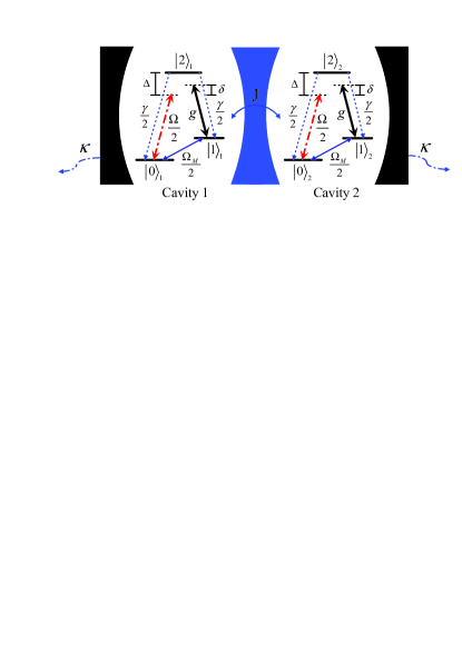
Figure 1: (Color online) Experimental setup for dissipative preparation of entangled steady-state between two $\Lambda$-type atoms trapped in two coupled cavities. The atom in each detuned cavity has two ground states $|1\rangle$ and $|0\rangle$, and one excited state $|2\rangle$, which is driven by the same off-resonance optical laser. The microwave fields applied to the two atoms differ by a relative phase of $\theta_{M}$.

The Hamiltonian $H_{0}$ describes the asymmetric coupling for the two atoms to the delocalized field mode $c_{1}$ and the symmetric coupling to $c_{2}$. Due to the photon hopping these two delocalized field modes are nondegenerate and each induces a collective atomic decay channel. The photon decay rate of cavity $i$ ($i$ = $1,2$) is denoted as $\kappa_{i}$ and the spontaneous emission rate of the atoms is denoted as $\gamma_{j}$ ($j$ = $1,2,3,4$). Under the condition $\kappa_{1}$ = $\kappa_{2}$ =$\kappa$, the Lindblad operators associated with the cavity decay and atomic spontaneous emission can be expressed as $L^{\kappa_{1}}$ = $\sqrt{\kappa}$ $c_{1}$, $L^{\kappa_{2}}$ = $\sqrt{\kappa}$ $c_{2}$, $L^{\gamma_{1}}$ = $\sqrt{\gamma_{1}}$ $|0\rangle_{1}\langle 2|$, $L^{\gamma_{2}}$ = $\sqrt{\gamma_{2}}$ $|0\rangle_{2}\langle 2|$, $L^{\gamma_{3}}$ = $\sqrt{\gamma_{3}}$ $|1\rangle_{1}\langle 2|$, $L^{\gamma_{4}}$ = $\sqrt{\gamma_{4}}$ $|1\rangle_{2}\langle 2|$. We assume $\gamma_{1}$ = $\gamma_{2}$ = $\gamma_{3}$ = $\gamma_{4}$ = $\gamma/2$ for simplicity.

Under the condition of weak classical laser field, we can adiabatically eliminate the excited cavity field modes and excited states of the atoms when the excited states are not initially populated. To tailor the effective decay processes to achieve a desired steady-state, we introduce an effective operator formalism based on second-order perturbation theory PRL2011-106-090502 ; arXiv1110.1024v1 ; arXiv:1112.2806v1 . Then the dynamics of our coupled cavity system is governed by the effective Hamiltonian $H_{eff}$ and effective Lindblad operator $L_{eff}^{x}$

$$H_{eff} = -\frac{1}{2}V_{-}[H^{-1}_{NH}+(H^{-1}_{NH})^{{\dagger}}]V_{+}+H_{g},$$ (8)

$$L_{eff}^{x} = L^{x}H^{-1}_{NH}V_{+},$$ (9)

where $H^{-1}_{NH}$ is the inverse of the non-Hermitian Hamiltonian $H_{NH}$ = $H_{0}$ $-$ $\frac{i}{2}\sum_{x}(L^{x})^{{\dagger}}L^{x}$.

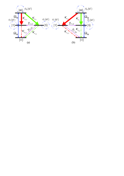
Figure 2: (Color online) Two effective models for coherent and dissipative interactions among states $|00\rangle$, $|S\rangle$ ($|T\rangle$) and $|11\rangle$, where two microwave fields cause rapid transitions. The atoms decay through the cavity from $|00\rangle$ to $|T\rangle$ and $|S\rangle$ with effective decay rates $\kappa_{c_{1,1}}$ and $\kappa_{c_{2,1}}$, and from $|T\rangle$ and $|S\rangle$ to $|11\rangle$ with the effective decay rates $\kappa_{c_{1,2}}$ and $\kappa_{c_{2,2}}$, where $\kappa_{c_{1,1}}$ $\gg$ $\kappa_{c_{1,2}}$ and $\kappa_{c_{2,1}}$ $\gg$ $\kappa_{c_{2,2}}$. $\gamma_{S,12}$, $\gamma_{S,34}$, $\gamma_{T,12}$ and $\gamma_{T,34}$ are the effective spontaneous emission rates. The loop-like element $O_{X}(\Omega^{2})$ ($X=00,S,T$) represents the square of the coefficient in the corresponding term $|X\rangle\langle X|$ within $H_{eff}$ without considering $H_{g}$. (a) $\theta_{M}=0$. (b) $\theta_{M}=\pi$.

The resulting effective master equation in Lindblad form is

$$\dot{\rho} = i[\rho,H_{eff}]+\sum_{x}\{L_{eff}^{x}\rho(L_{eff}^{x})^{{\dagger}}-\frac{1}{2}[(L_{eff}^{x})^{{\dagger}}L_{eff}^{x}\rho$$ (11)

$$+\rho(L_{eff}^{x})^{{\dagger}}L_{eff}^{x}]\},$$

$$H_{eff} = -Re[\frac{\Omega^{2}}{4}\widetilde{R}_{3}]|S\rangle\langle S|-Re[\frac{\Omega^{2}}{4}\widetilde{R}_{2}]|T\rangle\langle T|$$ (13)

$$-Re[\frac{\Omega^{2}}{2}\widetilde{R}_{1}]|00\rangle\langle 00|+H_{g},$$

$$L_{eff}^{\kappa_{1}} = \sqrt{\frac{(\delta+J)^{2}g_{eff}^{2}\kappa/4}{A_{\kappa_{1}}^{2}+B_{\kappa_{1}}^{2}}}|S\rangle\langle 00|+\sqrt{\frac{g_{eff}^{2}\kappa/4}{C_{\kappa_{1}}^{2}+D_{\kappa_{1}}^{2}}}|11\rangle\langle S|,$$ (14)

$$L_{eff}^{\kappa_{2}} = \sqrt{\frac{(\delta-J)^{2}g_{eff}^{2}\kappa/4}{A_{\kappa_{2}}^{2}+B_{\kappa_{2}}^{2}}}|T\rangle\langle 00|+\sqrt{\frac{g_{eff}^{2}\kappa/4}{C_{\kappa_{2}}^{2}+D_{\kappa_{2}}^{2}}}|11\rangle\langle T|,$$ (16)

where $Re[$ $]$ denotes the real part of the argument,

$$g_{eff} = \frac{g\Omega}{\Delta},\delta^{{}^{\prime}}=\delta-\frac{i}{2}\kappa,\Delta^{{}^{\prime}}=\Delta-\frac{i}{2}\gamma,$$ (18)

$$\widetilde{R}_{1} = \frac{-(\delta^{{}^{\prime}}-J)(\delta^{{}^{\prime}}+J)}{\delta^{{}^{\prime}}g^{2}-\Delta^{{}^{\prime}}(\delta^{{}^{\prime}}-J)(\delta^{{}^{\prime}}+J)},$$ (20)

$$\widetilde{R}_{2} = \frac{-gJ-\delta^{{}^{\prime}}g^{2}+\Delta^{{}^{\prime}}(\delta^{{}^{\prime}}-J)(\delta^{{}^{\prime}}+J)}{[g^{2}-\Delta^{{}^{\prime}}(\delta^{{}^{\prime}}-J)][g^{2}-\Delta^{{}^{\prime}}(\delta^{{}^{\prime}}+J)]},$$ (21)

$$\widetilde{R}_{3} = \frac{gJ-\delta^{{}^{\prime}}g^{2}+\Delta^{{}^{\prime}}(\delta^{{}^{\prime}}-J)(\delta^{{}^{\prime}}+J)}{[g^{2}-\Delta^{{}^{\prime}}(\delta^{{}^{\prime}}-J)][g^{2}-\Delta^{{}^{\prime}}(\delta^{{}^{\prime}}+J)]},$$ (22)

$$A_{\kappa_{1}} = A_{\kappa_{2}}=\frac{\delta g^{2}}{\Delta}-(\delta^{2}-J^{2}),$$ (23)

$$B_{\kappa_{1}} = B_{\kappa_{2}}=\kappa(\delta-\frac{g^{2}}{2\Delta})+\frac{\gamma(\delta^{2}-J^{2})}{2\Delta},$$ (24)

$$C_{\kappa_{1}} = \frac{g^{2}}{\Delta}-(\delta-J),D_{\kappa_{1}}=\frac{\kappa}{2}+\frac{\gamma(\delta-J)}{2\Delta},$$ (25)

$$C_{\kappa_{2}} = \frac{g^{2}}{\Delta}-(\delta+J),D_{\kappa_{2}}=\frac{\kappa}{2}+\frac{\gamma(\delta+J)}{2\Delta}.$$ (26)

As shown in Fig. 2 (a) and (b), the loop-like elements $O_{00}(\Omega^{2})$, $O_{T}(\Omega^{2})$ and $O_{S}(\Omega^{2})$ represent the effective-Hamiltonian evolution in three triplet states $|00\rangle$, $|T\rangle$ and $|S\rangle$ without microwave fields, respectively. For weak optical driving $\Omega$, $H_{eff}$ $\simeq$ $H_{g}$. There exist two effective decay channels characterized by $L_{eff}^{\kappa_{1}}$ and $L_{eff}^{\kappa_{2}}$ through the two delocalized bosonic modes $c_{1}$ and $c_{2}$ as compared with the case of Ref. PRL2011-106-090502 in which only one decay channel is mediated. It is the photon hopping that lifts the degeneracy of the two delocalized field modes and leads to the two independent decay channels. $L_{eff}^{\kappa_{1}}$ indicates the effective decay from $|00\rangle$ to $|S\rangle$ at a rate $\kappa_{c_{1,1}}$ and from $|S\rangle$ to $|11\rangle$ at a rate $\kappa_{c_{1,2}}$ caused by asymmetric $c_{1}$ mode, and $L_{eff}^{\kappa_{2}}$ denotes the effective decay from $|00\rangle$ to $|T\rangle$ at a rate $\kappa_{c_{2,1}}$ and from $|T\rangle$ to $|11\rangle$ at a rate $\kappa_{c_{2,2}}$ caused by symmetric $c_{2}$ mode simultaneously. The decay rates $\kappa_{c_{1,1}}$ ($\kappa_{c_{1,2}}$) and $\kappa_{c_{2,1}}$ ($\kappa_{c_{2,2}}$) equal to the square of the first (second) coefficient in the right side of Eq. (9) and Eq. (10), respectively. Set $A_{\kappa_{1}}$ $=$ $A_{\kappa_{2}}$ $=$ $0$, decays from $|S\rangle$ to $|11\rangle$ and from $|T\rangle$ to $|11\rangle$ can be both largely suppressed. On the other hand, the microwave fields drive the transition between the three states $|00\rangle$, $|T\rangle$ ($|S\rangle$) and $|11\rangle$ for $\theta_{M}=0(\pi)$. The dynamics of the full master equation in Fig. 3 (a) and (b) illustrates that we can obtain state $|S\rangle$ or $|T\rangle$ of high fidelity, and the time needed for reaching the entangled steady-state $|T\rangle$ is about two times as large as that of $|S\rangle$. This is because that the optimal ratio of $\kappa_{c_{1,1}}$/$\kappa_{c_{1,2}}$ is about $2$ times as large as $\kappa_{c_{2,1}}$/$\kappa_{c_{2,2}}$.

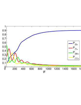
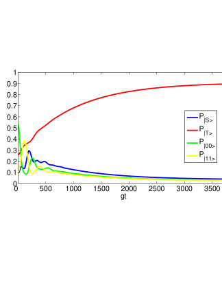
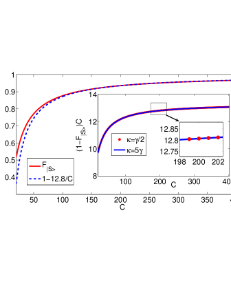
Figure 3: (Color online) The populations of four states $|S\rangle$, $|T\rangle$, $|00\rangle$ and $|11\rangle$ versus the dimensionless parameter $gt$ for a random initial state. Both curves are plotted for $C=200$, $\kappa=\gamma/2$, $\Omega_{M}=2\Omega/5$, $\Omega=g/20$ with $\Delta$, $\delta$ and $J$ being the optimal values for two entangled steady-states. (a) $\theta_{M}=0$. (b) $\theta_{M}=\pi$. (c) The fidelity $F_{|S\rangle}$ for steady-state $|S\rangle$ versus $C$, and the coefficient of the linear scaling in $F_{|S\rangle}$ as a function of $C$ with different ratios $\kappa/\gamma$ is plotted in the inset.

The errors imposed by all possible atomic spontaneous emissions should also be taken into account. We apply Eq. (6) again to derive four analytic expressions of effective spontaneous emissions with the other Lindblad operators $L^{\gamma_{1}}$, $L^{\gamma_{2}}$, $L^{\gamma_{3}}$ and $L^{\gamma_{4}}$

$$L^{\gamma_{1}}_{eff} = \sqrt{\frac{\gamma}{2}}[\frac{\Omega}{2}|\widetilde{R}_{1}||00\rangle\langle 00|+\frac{\Omega}{4}|\widetilde{R}_{2}|(|T\rangle\langle T|+|S\rangle\langle T|)$$ (28)

$$+\frac{\Omega}{4}|\widetilde{R}_{3}|(|T\rangle\langle S|+|S\rangle\langle S|)],$$

$$L^{\gamma_{3}}_{eff} = \sqrt{\frac{\gamma}{2}}[\frac{\Omega}{2\sqrt{2}}|\widetilde{R}_{1}|(|T\rangle\langle 00|+|S\rangle\langle 00|)$$ (30)

$$+\frac{\Omega}{2\sqrt{2}}(|\widetilde{R}_{2}||11\rangle\langle T|+|\widetilde{R}_{3}||11\rangle\langle S|)],$$

where $|\cdot|$ denotes modulus of the symbol in it, $L^{\gamma_{2}}_{eff}=L^{\gamma_{1}}_{eff}$ and $L^{\gamma_{4}}_{eff}=L^{\gamma_{3}}_{eff}$. The operators of effective spontaneous emission for $|S\rangle$ state are

$$L^{\gamma_{1}}_{eff,S} = L^{\gamma_{2}}_{eff,S}=\sqrt{\gamma_{S,i=1,2}}|T\rangle\langle S|,$$ (31)

$$L^{\gamma_{3}}_{eff,S} = L^{\gamma_{4}}_{eff,S}=\sqrt{\gamma_{S,i=3,4}}|11\rangle\langle S|,$$ (32)

and the operators of that for $|T\rangle$ state are

$$L^{\gamma_{1}}_{eff,T} = L^{\gamma_{2}}_{eff,T}=\sqrt{\gamma_{T,i=1,2}}|S\rangle\langle T|,$$ (33)

$$L^{\gamma_{3}}_{eff,T} = L^{\gamma_{4}}_{eff,T}=\sqrt{\gamma_{T,i=3,4}}|11\rangle\langle T|,$$ (34)

where

$$\gamma_{eff} \simeq \frac{(\frac{\gamma\Omega^{2}}{2})\{(gJ)^{2}+[\kappa(\Delta\delta-\frac{g^{2}}{2})+\gamma\frac{(\delta^{2}-J^{2})}{2}]^{2}\}}{(g^{2}-\Delta\delta)^{2}(g^{4}+\kappa^{2}\Delta^{2})},$$ (35)

and $\gamma_{S,i=1,2}$ $=$ $\gamma_{T,i=1,2}$ $=$ $\gamma_{eff}/16$, $\gamma_{S,i=3,4}$ $=$ $\gamma_{T,i=3,4}$ $=$ $\gamma_{eff}/8$. Then we use the rate equation to evaluate the fidelity for the state $(j=S$ or $T)$

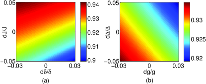
Figure 4: (Color online) $F_{|S\rangle}$ in the effective two-qubit system versus fluctuations of various parameters. (a) $F_{|S\rangle}$ vs $\frac{dJ}{J}$ and $\frac{d\delta}{\delta}$; (b) $F_{|S\rangle}$ vs $\frac{d\Delta}{\Delta}$ and $\frac{dg}{g}$.

$$\dot{P}_{j}=\kappa_{a}P_{00}-(\kappa_{b}+\sum_{i=1}^{4}\gamma_{j,i})P_{j},$$ (37)

where $P_{j}$ is the probability to be in the state $j$. The first term on the right side of Eq. (19) represents the population decaying into the state $j$ with the rate $\kappa_{a}$, while the other terms express the population leaking out of the state $j$ with the rate $\kappa_{b}+\sum_{i=1}^{4}\gamma_{j,i}$. Suppose $P_{j}$ $\simeq$ $1$ and the probability in each of the other three states is nearly $P_{00}$, then

$$1-F_{|S\rangle}\approx(3\frac{g_{eff}^{2}\kappa}{C_{k_{1}}^{2}+D_{k_{1}}^{2}}+9\gamma_{eff})/[\frac{(\delta+J)^{2}g_{eff}^{2}\kappa}{A_{k_{1}}^{2}+B_{k_{1}}^{2}}],$$ (38)

where $F_{|S\rangle}$ $=$ $|\langle S|\rho_{SS}|S\rangle|$ is the fidelity of state $|S\rangle$. Setting $\delta g^{2}=\Delta(\delta^{2}-J^{2})$ and $\kappa(\Delta\delta-g^{2}/2)$ $\simeq$ $\gamma(\delta^{2}-J^{2})/2$, the optimal fidelity of the entanglement can be obtained. The effective two-qubit system in the inset of Fig. 3 (c) shows that the fidelity scaling of state $|S\rangle$ is independent of different ratios $\kappa/\gamma$, then we find out the actual constants for maximizing the fidelity as follows

$$1-F_{|S\rangle}\approx 12.8C^{-1}.$$ (40)

The influences of different parameter fluctuations on the fidelity $F_{|S\rangle}$ of entangled state are considered. As shown in Fig. 4 (a) and (b), $F_{|S\rangle}$ keeps above $90\%$ even $5\%$ fluctuations in these parameters. The preparation process of state $|T\rangle$ is similar to that of $|S\rangle$.

Photonic band gap cavities coupled to atoms or quantum dots are suitable candidates for realizing the proposal. Cooperativity of value $C$ $\sim$ $100$ has been realized Nature2007-445-896 . The cavity modes can be coupled via the overlap of their evanescent fields or via an optical fiber, and photon hopping between two cavities has been observed PRB2000-61-R11855 .

In conclusion, we have proposed a scheme for dissipative preparation of entanglement between two atoms that are distributed in two coupled cavities. We find the linear scaling of the fidelity is a quadratic improvement compared with distributed entangled state preparation protocols based on unitary dynamics.

L.T.S., X.Y.C., H.Z.W, and S.B.Z acknowledge support from the National Fundamental Research Program Under Grant No. 2012CB921601, National Natural Science Foundation of China under Grant No. 10974028, the Doctoral Foundation of the Ministry of Education of China under Grant No. 20093514110009, and the Natural Science Foundation of Fujian Province under Grant No. 2009J06002. Z.B.Y is supported by the National Basic Research Program of China under Grants No. 2011CB921200 and No. 2011CBA00200, and the China Postdoctoral Science Foundation under Grant No. 20110490828.

References

(1) A. Einstein et al., Phys. Rev. 47, 777 (1935).
(2) B. W. Shore et al., J. Mod. Opt.
40, 1195 (1993).
(3) S. B. Zheng and G. C. Guo, Phys. Rev. Lett. 85, 2392 (2000).
(4) M. A. Nielsen et al., Quantum
Computation and Quantum Information (Cambridge Univ. Press, 2000).
(5) M. J. Kastoryano, F. Reiter, and A. S. Sørensen, Phys. Rev. Lett. 106, 090502 (2011).
(6) F. Reiter, M. J. Kastoryano, and A. S. Sørensen, arXiv:1110.1024v1.
(7) J. Busch, S. De et al., Phys. Rev. A 84, 022316 (2011).
(8) X. T. Wang and S. G. Schirmer, arXiv:1005.2114v2.
(9) L. Memarzadeh and S. Mancini, Phys. Rev. A 83, 042329 (2011).
(10) K. G. H. Vollbrecht, C. A. Muschik, and J. I. Cirac, Phys. Rev. Lett. 107, 120502 (2011).
(11) A. F. Alharbi and Z. Ficek, Phys. Rev. A 82, 054103 (2010).
(12) Z. Q. Yin et al., Phys. Rev. A 76, 062311 (2007).
(13) D. G. Angelakis et al., Eur. Phys. Lett. 85, 20007 (2009).
(14) D. Braun, Phys. Rev. Lett. 89, 277901 (2002).
(15) F. Benatti, R. Floreanini, and M. Piani, Phys. Rev. Lett. 91, 070402 (2003).
(16) K. L. Liu and H. S. Goan, Phys. Rev. A 76, 022312 (2007).
(17) C. H. Chou et al., Phys. Rev. E 77, 011112 (2008).
(18) F. Benatti and R. Floreanini, J. Phys. A 39, 2689 (2006).
(19) C. Horhammer and H. Buttner, Phys. Rev. A 77, 042305 (2008).
(20) J. P. Paz and A. J. Roncaglia, Phys. Rev. Lett. 100, 220401 (2008).
(21) H. Krauter et al., Phys. Rev. Lett. 107, 080503 (2011).
(22) C. D. Ogden et al., Phys. Rev. A 78, 063805 (2008).
(23) M. J. Hartmann et al., Laser Photon. Rev. 2, 527 (2008).
(24) C. DiFidio and W. Vogel, Phys. Rev. A 79, 050303(R) (2009).
(25) J. Cho et al., Phys. Rev. A 78, 022323 (2008).
(26) D. G. Angelakis et al., Phys. Rev. A 76, 031805(R) (2007).
(27) M. J. Hartmann et al., Nat. Phys. 2, 849 (2006).
(28) A. D. Greentree et al., Nat. Phys. 2, 856 (2006).
(29) D. K. Armani et al., Nature
421, 925 (2003).
(30) S. Clark et al., Phys. Rev. Lett. 91, 177901 (2003).
(31) Z. B. Yang, Y. Xia et al., Opt. Commu.
283, 3052 (2010).
(32) F. Reiter and A. S. Sørensen, arXiv:1112.2806v1.
(33) K. Hennessy et al., Nature 445, 896 (2007).
(34) M. Bayindir et al., Phys. Rev. B 61, R11855 (2000).