Mechanical surface tension governs membrane thermal fluctuations

Abstract

Motivated by the still ongoing debate about the various possible meanings of the term surface tension of bilayer membranes, we present here a detailed discussion that explains the differences between the “intrinsic”, “renormalized”, and “mechanical” tensions. We use analytical considerations and computer simulations to show that the membrane spectrum of thermal fluctuations is governed by the mechanical and not the intrinsic tension. Our study highlights the fact that the commonly used quadratic approximation of Helfrich effective Hamiltonian is not rotationally invariant. We demonstrate that this non-physical feature leads to a calculated mechanical tension that differs dramatically from the correct mechanical tension. Specifically, our results suggest that the mechanical and intrinsic tensions vanish simultaneously, which contradicts recent theoretical predictions derived for the approximated Hamiltonian.

I Introduction

Bilayer membranes are quasi-two-dimensional (2D) fluid sheets formed by spontaneous self-assembly of lipid molecules in water israelachvili . Their elasticity is traditionally studied in the framework of the Helfrich effective surface Hamiltonian for 2D manifolds with local principle curvatures $c_{1}$ and $c_{2}$ helfrich:73

$${\cal H}_{0}=\int_{A}dS\left[\sigma_{0}+\frac{1}{2}\kappa_{0}\left(c_{1}+c_{2}-2c_{0}\right)^{2}+{\bar{\kappa}}_{0}c_{1}c_{2}\right],$$ (1)

where the integration is carried over the whole surface of the membrane. The Helfrich Hamiltonian involves four parameters: the spontaneous curvature $c_{0}$, the surface tension $\sigma_{0}$, the bending modulus $\kappa_{0}$, and the saddle-splay modulus $\bar{\kappa}_{0}$. For symmetric bilayer membranes, $c_{0}=0$. If, in addition, the discussion is limited to deformations that preserve the topology of the membrane, then (by virtue of the Gauss-Bonnet theorem) the total energy associated with the last term is a constant, and one arrives to the more simple form

$${\cal H}_{0}=\int_{A}dS\left[\sigma_{0}+\frac{1}{2}\kappa_{0}\left(c_{1}+c_{2}\right)^{2}\right]=\sigma_{0}A+\frac{1}{2}\kappa_{0}J^{2},$$ (2)

where $A$ is the total area of the membrane and $J$, defined by $J^{2}=\int dS\left(c_{1}+c_{2}\right)^{2}$, is the integrated total curvature.

The surface tension appearing in Eq.(2) is known as the “intrinsic tension”. It represents the elastic energy required to increase the surface of the membrane by a unit area, and can be identified with the derivative of the energy with respect to the area $A$, $\sigma_{0}=(\partial{\cal H}/\partial A)$, at constant $J$. As this quantity is not directly measurable, its physical meaning is still a matter of a fierce debate. In molecular simulations, one can attach the membrane to a “frame” and measure the “mechanical (frame) tension”, $\tau$, which is the lateral force per unit length exerted on the boundaries of the membrane goets:98 ; lindahl:00 ; grace:05 ; neder:10 . Experimentally, the mechanical tension is routinely measured by micropipette aspiration of vesicles rawicz:90 ; rawicz:00 . Formally, the mechanical tension is obtained by taking the full derivative of the free energy $F$ with respect to the frame (projected) area: $\tau=dF/dA_{p}$ remark1 . From a comparison of the above definitions of $\sigma_{0}$ and $\tau$, it becomes clear that the intrinsic and mechanical tensions are different quantities. Contrary the former, the latter is a thermodynamic quantity that also depends on the entropy of the membrane. Bilayer membranes usually exhibit relatively large thermal undulations at room temperature safran and, indeed, their mechanical tension also includes an entropic contribution due to the suppression of the amplitude of the undulations upon increasing the projected area.

The surface tension can be also measured indirectly by recording and analyzing the statistics of the membrane height fluctuations duwe:90 ; dobereiner:03 . The analysis is based on the so called Monge parametrization, where the surface of the fluctuating membrane is represented by a height function, $h(x,y)$, above the frame $(x,y)$ plane. The Helfrich Hamiltonian does not have a simple form when expressed in terms of $h(x,y)$. However, for a nearly flat membrane, i.e., when the derivatives of $h$ with respect to $x$ and $y$ are small ($|\partial_{x}h|,\ |\partial_{y}h|\ll 1$), one obtains the quadratic approximation

$${\cal H}^{M}_{2}=\sigma_{0}A_{p}+\int dxdy\left[\frac{\sigma_{0}}{2}\left(\nabla h\right)^{2}+\frac{\kappa_{0}}{2}\left(\nabla^{2}h\right)^{2}\right].$$ (3)

Note that unlike Eq.(2), the integral in Eq.(3) runs over the frame area rather than over the area of the manifold. The quadratic approximation can be diagonalized by introducing the Fourier transformation: $h_{q}=(1/A_{p})\int dxdy\,h(x,y)\exp(-i\vec{q}\cdot\vec{r})$. In Fourier space the Hamiltonian reads

$${\cal H}^{M}_{2}=\sigma_{0}A_{p}+\frac{A_{p}}{2}\sum_{\vec{q}}\left(\sigma_{0}q^{2}+\kappa_{0}q^{4}\right)|h_{q}|^{2},$$ (4)

and by invoking the equipartition theorem, we find that the mean square amplitude of mode $\vec{q}$ (“spectral intensity”):

$$\langle|h_{q}|^{2}\rangle=\frac{k_{B}T}{A_{p}(\sigma_{0}q^{2}+\kappa_{0}q^{4})}.$$ (5)

From the last result, it seems as if $\sigma_{0}$ can be extracted from the fluctuation spectrum of the membrane. Results of both fully-atomistic and coarse-grained simulation marrink:01 ; farago:03 ; cooke:05 ; wang:05 ; boek:05 show that spectral intensity can indeed be fitted to the form

$$\langle|h_{q}|^{2}\rangle=\frac{k_{B}T}{A_{p}(rq^{2}+{\cal O}(q^{4}))}$$ (6)

However, the derivation of Eq.(5) is based on the approximated Hamiltonian ${\cal H}^{M}_{2}$ and, therefore, it is not a-priory clear why the so called “$q^{2}$-coefficient” appearing in Eq.(6), $r=\sigma_{0}$. In fact, some theoretical studies have argued that the $q^{2}$ coefficient is actually equal to the mechanical tension $\tau$ cai:94 ; farago_pincus:04 ; schmid:11 . This conclusion has been rejected more recently in favor of the more common interpretation that $r=\sigma_{0}$ imparato:06 ; fournier:08 . Membrane simulations carried at fixed mechanical tension (usually performed for $\tau=0$) tend to agree with the result that $r=\tau$ lindahl:00 ; marrink:01 ; cooke:05 ; wang:05 ; farago:08 , but simulations that show the opposite $r\neq\tau$ also exist imparato:06 ; stecki:06 . In this paper we settle this problem and prove, analytically and computationally, that the correct result is indeed $r=\tau$.

II What does the intrinsic tension represent?

Much of the confusion associated with the physical meaning of surface tension in membranes is related to fact that the concept of surface tension has been originally defined for an interface between bulk phases (e.g., between water and oil) rowlinson_widom . In its original context, the surface tension represents the access free energy $\Delta F$ per unit area $A$ of the interface between the bulk phases

$$\gamma=\frac{\Delta F}{A}.$$ (7)

When the concept of surface tension is introduced into the theory of bilayer membranes, its meaning is distorted due to the following two major differences between membranes and interfaces of bulk phases

1. In the case of bulk phases, it is often assumed that the interface between them is flat. There is usually very little interest in the thermal roughness of the interface, unless it is very soft. In contrast, bilayer membranes are treated as highly fluctuating surfaces whose elastic response is very much influenced by the entropy associated with the thermal fluctuations.

2. The changes in the areas of both systems arise from very different origins. In the case of, say, a water-oil interface, the changes in the interfacial area are not produced by elastic deformations (dilation/compression) that modify the molecular densities of the bulk phases. Instead, they result from transfer of molecules between the bulk phases and the interface occurring, for instance, when the shape of the container is changed. The surface tension $\gamma$ is essentially a chemical potential which is directly related to the exchange parameter between the coexisting phases dill . The case of bilayer membranes is completely different. Here, there is an exchange of water between the bulk fluid and interfacial region, but almost no exchange of lipid material because the concentration of free lipids in the embedding solution is extremely low ($10^{-6}-10^{-10}$ M israelachvili ). In other words, there is no reservoir of lipids outside of the bilayer and, therefore, a changes in the bilayer area result in a change in the area density of the lipids. The membrane surface tension measures the response to this elastic deformation, including the indirect contribution due to the exchange of water between the bilayer and solution resulting from the deformation (which has influence on the effective elastic moduli).

Most earlier theoretical investigations of membranes involved the assumption that the area per lipid $a$ is constant. This assumption relies on the observation that the energy cost involved in density fluctuations is much larger than the energy scale associated with curvature fluctuations. Further assuming that the lipids are insoluble in water (and, therefore, they all reside on the membrane where their number $N$ is constant) implies that the total area of the membrane $A=Na$ is constant. If that is the case, then why does one need to include this constant in the Helfrich Hamiltonian [first term on the right hand side of Eq.(2)], and what does the coefficient, $\sigma_{0}$, represent? The answer is simple. It is technically very hard to calculate analytically the partition function for a fluctuating manifold with a fixed area $A$. The first term in Eq.(2) is a Lagrange multiplier that fixes the mean area $\langle A\rangle$ of the membrane, and the value of $\sigma_{0}$ is set by the requirement that $A=\langle A\rangle=\partial F/\partial\sigma_{0}$. As usual, it is assumed that in the thermodynamic limit the relative fluctuations in the total area become negligible, and there is no distinction between $\langle A\rangle$ and $A$.

The renewed interest in the meaning of surface tension during the past decade is very much linked with the rapid development in computer modeling and simulations of bilayer membranes. In molecular simulations the number of lipids $N$ is usually fixed, but the total area in not. Membranes are no longer treated as incompressible thin films, but rather as stretchable/compressible surfaces whose elastic response result from their intermolecular forces. With this point of view in mind, it is clear that the intrinsic tension $\sigma_{0}$ in Helfrich Hamiltonian represents an elastic coefficient which, potentially, may be related to the mechanical tension $\tau$. There is, of course, no reason to expect that the elastic energy $E$ of the membrane is linear in $A$ remark_added . A quadratic elastic function $E=1/2K_{A}(A-A_{0})^{2}$ seems like a more appropriate form, where $K_{A}$ is the stretching/compression modulus and $A_{0}$ is the relaxed area of the membrane farago_pincus:03 (also known as Schulman’s area schulman ). Expressing the total area as the sum of the projected and undulations areas $A=A_{p}+\delta A$, and assuming that $\delta A\ll|A_{p}-A_{0}|$, yields the linear approximation $E\simeq 1/2K_{A}(A_{p}-A_{0})^{2}+K_{A}(A_{p}-A_{0})\delta A$ from which one identifies that $\sigma_{0}=K_{A}(A_{p}-A_{0})$. The assumption that $\delta A\ll|A_{p}-A_{0}|$ becomes increasingly accurate at high tensions; but, nevertheless, the linear relationship between $E$ and $A$ is used in Eq.(2) over the entire range of intrinsic tensions.

Figure 1: A fluctuating membrane with a projected area $A_{p}$ at four different states: (a) the reference undeformed state, (b) under shear deformation, (c) subjected to an arbitrary deformation, and (d) as in (c) but with periodic boundary conditions. Each state is characterized by the mean height profile function $\bar{h}(x,y)$ which is indicated by a thick solid line. The dashed thin line in (a) serves as a reminder that the membrane is fluctuating around its mean profile.

III Helfrich elastic free energy

The proof that $r=\tau$ consists of three steps and involves the introduction of two additional surface tensions: (i) $\sigma$, the renormalized surface tension, and (ii) $\mu$, the out-of-plane shear modulus (which, as it will turn out below, is also a surface tension). Let us first understand what these two quantities represent. The out-of-plane shear modulus $\mu$ is the force per unit length required to introduce the deformation depicted in fig. 1(b) from the initial reference state depicted in fig. 1(a). This deformation is achieved by applying opposite normal forces on boundaries of the membrane. (Notice that the out-of-plane shear deformation changes the area of the membrane, but preserves the volume of the three-dimensional Euclidean metric. We will revisit this point later in section III.3.) The shear modulus is not related to the deformation of a specific configuration but rather to the deformation of a fluctuating membrane. The out of plane shear is a special case of a more general family of elastic deformations resulting from the action of normal stress fields. A representative of this family of deformations is shown schematically in fig. 1(c). Mathematically, such deformations can be characterized by the mean height profile of the membrane: $\langle h(x,y)\rangle\equiv\bar{h}(x,y)$. This function, which vanishes in the undeformed reference state $\bar{h}(x,y)=0$, serves as the strain field that describes arbitrary deformations of the fluctuating membrane at fixed projected area $A_{p}$. Specifically for the shear deformation shown in fig. 1(b), $\bar{h}(x,y)=\epsilon x$ where $\epsilon$ is the shear strain. The normal stress field associated with the strain function $\bar{h}(x,y)$ can be derived from the elastic free energy $F(\bar{h})$. Based on the same physical arguments used to justify the introduction of Helfrich effective Hamiltonian Eq.(2), we hereby assume that the elastic free energy $F(\bar{h})$ can be written in a similar form

$$F\left(\bar{h}\left(x,y\right)\right)=\sigma\tilde{A}\left(\bar{h}\right)+\frac{1}{2}\kappa(\tilde{J})^{2}\left(\bar{h}\right),$$ (8)

where $\tilde{A}(\bar{h})$ and $\tilde{J}(\bar{h})$ are the total area and integrated total curvature of the mean height profile of the membrane, $\bar{h}(x,y)$. Our conjecture of Eq.(8) is based on the fact (which will be proved in the following section III.1) that this form of the free energy yields the experimentally and computationally well established Eq.(6) for the spectral intensity. The coefficient $\sigma$ and $\kappa$ appearing in Eq.(8) are the renormalized surface tension and bending rigidity. These quantities are thermodynamic properties of the membranes which, in general, include entropic contributions and, therefore, are different than the corresponding microscopic coefficients appearing in the Helfrich effective Hamiltonian.

III.1 Linear response theory

The first step in the proof that $r=\tau$ is to show that $r=\sigma$, which follows from static linear response theory. Detailed proof of this point can be found in ref. farago_pincus:04 ; here we provide a short version of the derivation. Let us consider an elastic deformation with a function $\bar{h}(x,y)$ that satisfies periodic boundary conditions (see, e.g., fig. 1(d)). Introducing $\bar{h}_{q}$, the Fourier transform of the function $\bar{h}(x,y)$, and expanding $\tilde{A}$ and $\tilde{J}$ in powers of $\bar{h}_{q}$, we find

$$F\left(\left\{\bar{h}_{q}\right\}\right)=\sigma A_{p}+\frac{A_{p}}{2}\sum_{\vec{q}}\left[\sigma q^{2}+\kappa q^{4}\right]\bar{h}_{q}\bar{h}_{-q}+{\cal O}\left(|\bar{h}_{q}|^{4}\right)$$ (9)

where $\bar{h}_{-q}=\bar{h}_{q}^{*}$ since the function $\bar{h}(x,y)$ is real remark2 .

Let us now consider the perturbed Hamiltonian ${\cal H}={\cal H}_{0}-\sum_{\vec{q}}j_{q}h_{q}$, where ${\cal H}_{0}$ is the Hamiltonian of the membrane. Notice that we do not need to know the specific form of ${\cal H}_{0}$ and, in particular, we do not assume here that ${\cal H}_{0}$ is necessarily the Helfrich Hamiltonian Eq.(2) or its quadratic approximation Eq.(3). Instead, we assume that the free energy is given by Eq.(8) [or by its Fourier space counterpart Eq.(9)]; and as we shall now show, this is the key assumption that ultimately leads to Eq.(6). The derivation is as follows: Introducing the Gibbs free energy $G(\{j_{q}\})=-k_{B}T\ln[{\rm Tr}\,\exp(-{\cal H}/k_{B}T)]$, and taking the derivative of $G$ with respect to $j_{q}$ yields

$$\bar{h}_{q}=-\frac{dG\left(\left\{j_{q}\right\}\right)}{dj_{q}}.$$ (10)

The conjugate thermodynamic variables $\bar{h}_{q}$ and $j_{q}$ can be also related to each other via

$$j_{q}=\frac{dF\left(\left\{\bar{h}_{q}\right\}\right)}{d\bar{h}_{q}},$$ (11)

which, by using Eq.(9) for the Helmholtz free energy $F$, reads

$$j_{q}=A_{p}\left(\sigma q^{2}+\kappa q^{4}\right)h_{-q}+{\cal O}\left(|\bar{h}_{q}|^{3}\right).$$ (12)

Deriving Eq.(10) with respect to $j_{-q}$ yields the relationship between the elastic linear response and the equilibrium fluctuations in $h_{q}$

$$\left\langle|h_{q}|^{2}\right\rangle_{0}=k_{B}T\frac{d\bar{h}_{q}}{dj_{-q}}{\Biggm{|}}_{j_{q}=0}=k_{B}T\left(\frac{dj_{-q}}{d\bar{h}_{q}}\right)^{-1}{\Biggm{|}}_{\bar{h}_{q}=0},$$ (13)

where $\langle\cdots\rangle_{0}$ denote a thermal average using the unperturbed Hamiltonian ${\cal H}_{0}$. Using Eq.(12) in Eq.(13), one arrives to the result that

$$\langle|h_{q}|^{2}\rangle=\frac{k_{B}T}{A_{p}(\sigma q^{2}+\kappa q^{4})}.$$ (14)

This completes the proof that $r=\sigma$ which, as noted above, is independent of the explicit form of ${\cal H}_{0}$.

III.2 The renormalized tension is a shear modulus

The second step is to prove that $\sigma=\mu$. This can be done easily by considering the shear deformation $\bar{h}(x,y)=\epsilon x$ shown in fig. 1(b). The out of plane shear modulus is defined by the expansion of the free energy density in powers of $\epsilon$

$$\frac{F}{A_{p}}=f_{0}+\frac{\mu}{2}\epsilon^{2}+{\cal O}(\epsilon^{4}).$$ (15)

(The expansion includes only even powers of $\epsilon$ because of the symmetry of the problem with respect to reflections in the direction normal to the projected area.). However, for the shear deformation, the mean profile is flat, i.e. $\tilde{J}=0$, and therefore Eq.(8) reads

$$F\left(\bar{h}\left(x,y\right)\right)=\sigma\tilde{A}.$$ (16)

The area $\tilde{A}$ and $\epsilon$ are related by $\tilde{A}=\sqrt{1+\epsilon^{2}}A_{p}=A_{p}[1+\epsilon^{2}/2+{\cal O}(\epsilon^{4})]$, which yields

$$\frac{F}{A_{p}}=f_{0}+\frac{\sigma}{2}\epsilon^{2}+\ldots\ .$$ (17)

Comparison of Eqs.(15) and (17) leads to the result $\sigma=\mu$ which, again, is independent of the explicit form of the membrane Hamiltonian ${\cal H}_{0}$.

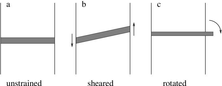
Figure 2: (a) The unstrained reference state of a thin film. (b) The film subjected to a simple shear deformation. (c) The film subjected to a pure shear deformation. The two deformed states have the same elastic free energy since they can be transformed into each other by rotation. The volume of the film (indicated by the gray shaded area) is the same at all three states.

III.3 Rotational invariance

Having demonstrated that $r=\sigma=\mu$, the last step in the proof that $r=\tau$ is to show that $\tau=\sigma=\mu$. This follows immediately from the invariance of Helfrich free energy Eq.(8) with respect to rigid transformations. Specifically, the sheared membrane which is replotted in fig. 2(b), can be rotated (see fig. 2(c)) so that the mean profile of the deformed membrane lies in the $(x,y)$ plane defined by the undeformed state (fig. 2(a)). In this orientation $\tilde{A}=A_{p}$, and from Eq.(16) one gets that the free energy cost of imposing the deformation in fig. 2(c) is $F=\sigma A_{p}$. From this result one finds that the mechanical tension

$$\tau=\frac{dF}{dA_{p}}=\sigma$$ (18)

.

While Eq.(18) is correct, it misses an important issue which cannot be captured within the framework of Helfrich model that treats the membrane as a 2D manifold with no 3D volume. In figs. 2(a)-(c) we have intentionally drawn the membranes as thin films, which highlights a very important point. The transition from the reference state (a) to the deformed state (c) is achieved via a sequence of two volume-preserving transformations - shear followed by rotation. Therefore, the reference state and the deformed one have different areas but the same volume, which means that in Eq.(18) one must take the derivative at a constant volume:

$$\tau=\frac{\partial F}{\partial A_{p}}\Biggm{|}_{V}=\mu.$$ (19)

Experimentally and computationally, there is no practical way to fix or even determine the volume of a bilayer at the molecular resolution. This, however, does not render the above argument irrelevant to lipid bilayer membranes. The membrane and the embedding fluid medium are placed in a “container” whose volume can be easily controlled. Eq.(19) states that the frame tension of the bilayer can be measured by changing the cross-sectional area of the container while keeping its volume fixed. This tension is associated with the entire “interfacial region” of the system that includes both the bilayer of lipids as well as the hydration layers of structured water around the bilayer. The fluid bulk water has no elastic response to volume preserving deformations and, therefore, it make no contribution to $\tau$.

The fact that $\tau$ is associated with a volume preserving deformation is important. The reader may have noticed that in Eq.(18) we wrote $\tau=\sigma$, while in Eq.(19) we preferred the equality $\tau=\mu$. Obviously, the latter is also correct since, as discussed above in section III.2, $\sigma=\mu$. In writing $\tau=\mu$ in Eq.(19) we wish to emphasize the fact that the frame tension is also a shear modulus. It represents the response of the system to “pure shear” deformations (fig. 2(c)), which is the same as the response to “simple shear” (fig. 2(b)). The modulus of pure shear can be derived by considering the free energy cost associated with changing the dimensions of a system from $L_{x}\times L_{y}\times L_{z}$ to $[L_{x}(1+\epsilon)]\times[L_{y}(1+\epsilon)]\times[L_{z}/(1+\epsilon)^{2}]$. The expansion of the free energy density in powers of $\epsilon$ reads

$$\frac{F}{L_{x}L_{y}L_{z}}=f_{0}+(2P_{z}-P_{x}-P_{y})\epsilon+{\cal O}(\epsilon^{2}),$$ (20)

where $P_{i}$ is the pressure along the $i$-th Cartesian axis. Due to the deformation, the projected area $A_{p}=L_{x}L_{y}$ changes by $\Delta A_{p}\simeq 2A_{p}\epsilon$. Therefore, Eq.(20) can also be written as

$$F=F_{0}+L_{z}\Delta A_{p}\left[P_{z}-\frac{P_{x}+P_{y}}{2}\right]+{\cal O}\left(\left(\Delta A_{p}\right)^{2}\right),$$ (21)

and the frame tension is given by

$$\tau=\lim_{\Delta A_{p}\rightarrow 0}\frac{F-F_{0}}{\Delta A_{P}}=L_{z}\left[P_{z}-\frac{P_{x}+P_{y}}{2}\right]=L_{z}\left[P_{n}-P_{t}\right],$$ (22)

where $P_{n}$ and $P_{t}$ are, respectively, the normal and transverse components of the pressure tensor (the negative Cauchy stress tensor) relative to the plane of the membrane. Eq.(22) is known as the mechanical definition of the surface tension rowlinson_widom .

III.4 The approximated Hamiltonian

At this point only one question is left: why does one get $r=\sigma_{0}$ rather than $r=\tau$ when dealing with the quadratic approximation of the effective surface Hamiltonian, Eq.(3)? The answer is simple - the approximated Hamiltonian is not rotationally invariant. This striking fact (which has been discussed by Grinstein and Pelcovitz in the context of lamellar liquid crystalline phases grinstein:81 ) can be demonstrated by considering a certain configuration parametrized by the height function $h(x,y)$ which satisfies periodic boundary conditions, and evaluating the elastic energy cost corresponding to simple and pure shear deformations. As discussed above, the result that $r=\mu$ is Hamiltonian-independent, but the following conclusion that $\mu=\tau$ depends on rotational invariance, i.e., on the fact that the two shear deformations result in the same elastic response. This, unfortunately, is not the case with Eq.(3). For the simple shear deformation $h_{\mu}(x,y)=h(x,y)+\epsilon x$, and upon substituting $h_{\mu}(x,y)$ in Eq.(3) one gets

$${\cal H}^{M}_{2}\left(h_{\mu}\left(x,y\right)\right)=\sigma_{0}A_{p}+\int dxdy\left[\frac{\sigma_{0}}{2}\left(\nabla h_{\mu}\right)^{2}+\frac{\kappa_{0}}{2}\left(\nabla^{2}h_{\mu}\right)^{2}\right]={\cal H}^{M}_{2}\left(h\left(x,y\right)\right)+\sigma_{0}A_{p}\frac{\epsilon^{2}}{2}.$$ (23)

From this result one finds that

$$\mu=\frac{1}{A_{p}}\frac{d^{2}\left\langle{\cal H}^{M}_{2}\left(h_{\mu}\left(x,y\right)\right)\right\rangle}{d\epsilon^{2}}=\sigma_{0},$$ (24)

and, thus, $r=\mu=\sigma_{0}$. This conclusion that $r=\sigma_{0}$ is in agreement with what the equipartition theorem Eq.(5) predicts for the approximated Hamiltonian. The response to pure shear is determined by considering the transformation $h_{\tau}(x^{\prime},y^{\prime})=h(x(1+\epsilon),y(1+\epsilon))/(1+\epsilon)^{2}$, with $0<x^{\prime}\leq L_{x}(1+\epsilon),\ 0<y^{\prime}\leq L_{y}(1+\epsilon)$. For this deformation: $A_{p}(\epsilon)=A_{p}(\epsilon=0)\cdot(1+\epsilon)^{2}$, $dx^{\prime}dy^{\prime}=(1+\epsilon)^{2}dxdy$, $\nabla h_{\tau}=\nabla h/(1+\epsilon)^{3}$, and $\nabla^{2}h_{\tau}=\nabla^{2}h/(1+\epsilon)^{4}$. When these relations are used in Eq.(3), we gets:

$${\cal H}^{M}_{2}\left(h_{\tau}\left(x,y\right)\right) = (1+\epsilon)^{2}\sigma_{0}A_{p}(\epsilon=0)+\int dx^{\prime}dy^{\prime}\left[\frac{\sigma_{0}}{2}\left(\nabla h_{\tau}\right)^{2}+\frac{\kappa_{0}}{2}\left(\nabla^{2}h_{\tau}\right)^{2}\right]=$$ (25)

$${\cal H}^{M}_{2}\left(h\left(x,y\right)\right) + 2\epsilon\sigma_{0}A_{p}(\epsilon=0)-\int dxdy\left[2\epsilon\sigma_{0}\left(\nabla h\right)^{2}+3\epsilon\kappa_{0}\left(\nabla^{2}h\right)^{2}\right]+{\cal O}(\epsilon^{2}).$$

From this result, one derives the mechanical tension, which is given by

$$\tau=\frac{1}{2A_{p}}\frac{d\left\langle{\cal H}^{M}_{2}\left(h_{\tau}\left(x,y\right)\right)\right\rangle}{d\epsilon}\Biggm{|}_{\epsilon=0}=\sigma_{0}-\frac{1}{A_{p}}\left\langle\int dxdy\left[\sigma_{0}\left(\nabla h\right)^{2}+\frac{3}{2}\kappa_{0}\left(\nabla^{2}h\right)^{2}\right]\right\rangle.$$ (26)

The second term on the right hand side of Eq.(26) is the entropic part of the mechanical tension, evaluated within the framework of the approximated quadratic Hamiltonian. This entropic contribution to $\tau$ is not reflected in the fluctuation spectrum of the quadratic Hamiltonian, which has the non-physical feature of not being rotationally invariant.

IV Computer simulations

To summarize our discussion: For any Hamiltonian whose corresponding free energy is given by the rotationally invariant free energy Eq.(8), the correct result is $r=\tau$. For the not rotationally invariant quadratic Hamiltonian Eq.(3), $r=\sigma_{0}\neq\tau$. In order to test these predictions, we performed Monte Carlo simulations of the one-dimensional (1D) analogs of Eqs.(2) and (3). Within these two models, the membrane is represented by a string of $N=1024$ points, the positions of which in 2D space are given by $\{\vec{r}_{i}=(x_{i},h_{i})\}$. In both cases, the simulations are performed at a constant projected length $L_{p}$ with periodic boundary conditions. Denoting by $\vec{b}_{i}=\vec{r}_{i+1}-\vec{r}_{i}$, the distance vector (“bond”) between adjacent points, the 1D analog of the rotationally invariant Helfrich effective Hamiltonian is given by remark3

$${\cal H}_{1}=\sigma_{0}\sum_{i}|\vec{b}_{i}|+\kappa_{0}\sum_{i}\left[1-\frac{\vec{b}_{i}\cdot\vec{b}_{i-1}}{|\vec{b}_{i}||\vec{b}_{i-1}|}\right].$$ (27)

The quadratic approximation of this Hamiltonian is given by

$${\cal H}_{2}=\sigma_{0}L_{p}+\frac{\sigma_{0}}{2l_{p}}\sum_{i}\left(h_{i+1}-h_{i}\right)^{2}+\frac{\kappa_{0}}{2l_{p}^{2}}\sum_{i}\left(h_{i+1}+h_{i-1}-2h_{i}\right)^{2},$$ (28)

where $l_{p}=L_{P}/N$. Notice that in the 1D models, the tension has units of a force (energy per unit length). A major difference between the two 1D models is related to the positions of the points. In the rotationally invariant case Eq.(27), the points are allowed to be anywhere in the available 2D space. At low tensions, this creates configurations in which the chain forms overhangs (see e.g., fig. 3(a)). The existence of such configurations does not invalidate any of the above discussion which only requires that the mean height profile $\bar{h}(x,y)$ is a well defined function. Within the quadratic approximation Eq.(28), the points are allowed to move only in the direction normal to the projected length [in the spirit of Eq.(3) in which the height is measured from the $x-y$ plane]. Thus, the position of the $i$-th point is given by $\vec{r}_{i}=(il_{p},h_{i})$ and, obviously, such moves do not generate any overhangs (see a typical configuration in fig. 3(b)).

In the simulations, we vary $\sigma_{0}$ and measure both the mechanical tension, $\tau$, and the $q^{2}$-coefficient, $r$. For each value of $\sigma_{0}$, the simulations extended over $2-4\times 10^{8}$ MC time units, where each time unit consists of $N$ single particle move attempts and one collective “mode excitation Monte Carlo” (MEMC) move that accelerates the very slow relaxation dynamics of the 10 largest Fourier modes memc . The introduction of MEMC moves is essential for the equilibration of the system. The mechanical tension is calculated using the 1D equivalent of Eq.(22), $\tau=f_{n}-f_{t}$, where $f_{n}$ and $f_{t}$ are the normal and transverse forces acting of the chain. Expressing these forces as thermal averages, one arrives to the following virial formulae. For the rotationally invariant Helfrich Hamiltonian ${\cal H}_{1}$

$$\tau = \left\langle\sum_{i}\left[\sigma_{0}\frac{\left(x_{i+1}-x_{i}\right)^{2}-\left(h_{i+1}-h_{i}\right)^{2}}{l_{p}|\vec{b}_{i}|}\right.\right.$$ (29)

$$+ \kappa_{0}\frac{2}{l_{p}|\vec{b}_{i-1}||\vec{b}_{i}|}\left(\frac{\left(h_{i}-h_{i-1}\right)\left(h_{i+1}-h_{i}\right)\left(x_{i}-x_{i-1}\right)^{2}-\left(x_{i}-x_{i-1}\right)\left(x_{i+1}-x_{i}\right)\left(h_{i}-h_{i-1}\right)^{2}}{|\vec{b}_{i-1}|^{2}}\right.$$

$$+ \left.\left.\left.\frac{\left(x_{i}-x_{i-1}\right)^{2}+\left(h_{i}-h_{i-1}\right)^{2}}{|\vec{b}_{i}|^{2}}\right)\right]\right\rangle.$$

For the approximated quadratic Hamiltonian ${\cal H}_{2}$

$$\tau = \sigma_{0}-\left\langle\sum_{i}\left[\frac{3\sigma_{0}}{2l_{p}^{2}}\left(h_{i+1}-h_{i}\right)^{2}+\frac{2\kappa_{0}}{l_{p}^{3}}\left(h_{i+1}+h_{i-1}-2h_{i}\right)^{2}\right]\right\rangle.$$ (30)

The $q^{2}$-coefficient $r$ is obtained by taking the Fourier transform of the the function $h_{i}$, and fitting the measurements to Eq.(6). Our results for $r$ are based on the analysis of the fluctuations of the 10 largest Fourier modes.

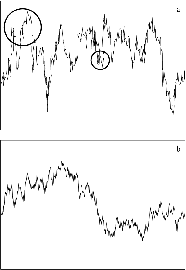
Figure 3: Typical configurations of the chain in (a) the rotationally invariant Hamiltonian Eq.(27), and (b) its quadratic approximation Eq.(28). Both configurations have been obtained for $\sigma_{0}=0.75k_{B}T/l_{p}$ and $\kappa_{0}=0$. In (a) the points of the chain are allowed be anywhere in the available 2D space which creates overhangs such as those shown inside the bold circles. In (b) the points move only vertically to the line that connects the end points of the chain.

Our simulation results for the quadratic Hamiltonian ${\cal H}_{2}$ are summarized in fig. 4. For both $\kappa_{0}=0$ and $\kappa_{0}=1k_{B}T$ and for all values of $\sigma_{0}$, we find that, indeed, all our measurements of the $q^{2}$-coefficient agree with the predicted relationship $r=\sigma_{0}$ (which is denoted by the dashed line). As expected from Eq.(30), the mechanical tension $\tau$ is smaller than $r$ and for small values of $\sigma_{0}$ even gets negative values. In comparison, the simulation results for the rotationally invariant Helfrich Hamiltonian ${\cal H}_{1}$ are shown in fig 5. In agreement with our expectations for this case, the various tensions satisfy the relationship that $r=\tau\neq\sigma_{0}$. To further demonstrate the validity of our discussion in section III, we computed the simple shear modulus $\mu$, which for Hamiltonian ${\cal H}_{1}$, is also expected to be equal to $r$ and $\tau$. The shear modulus $\mu$ can be computed using a rather cumbersome virial expression. For $\kappa_{0}=0$, the virial expression for $\mu$ takes the more simple form:

$$\mu=\left\langle\sum_{i}\sigma_{0}\frac{\left(x_{i+1}-x_{i}\right)^{4}}{l_{p}|\vec{b}_{i}|^{3}}-\frac{1}{l_{p}k_{B}T}\left(\sum_{i}\sigma_{0}\frac{\left(x_{i+1}-x_{i}\right)\left(h_{i+1}-h_{i}\right)}{|\vec{b}_{i}|}\right)^{2}\right\rangle.$$ (31)

Our results for $\mu$ agree perfectly with the results for $\tau$ and $r$.

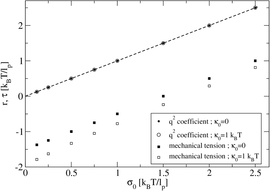
Figure 4: Simulation results for Hamiltonian ${\cal H}_{2}$ [Eq.(28)]: The $q^{2}$-coefficient $r$ (circles) and the mechanical tension $\tau$ (squares) as a function of the intrinsic tension $\sigma_{0}$. Results are shown for both $\kappa_{0}=0$ (solid symbols) and $\kappa_{0}=1k_{B}T$ (open symbols). The dashed line is a guide to the eye for the relationship $r=\sigma_{0}$.

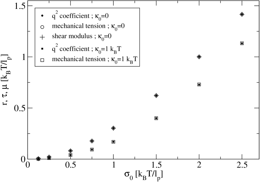
Figure 5: Simulation results for Hamiltonian ${\cal H}_{1}$ [Eq.(27)]: The $q^{2}$-coefficient $r$ (solid symbols) and the mechanical tension $\tau$ (open symbols) as a function of the intrinsic tension $\sigma_{0}$. Results are shown for both $\kappa_{0}=0$ (circles) and $\kappa_{0}=1k_{B}T$ (squares). The pluses denote our results for the shear modulus $\mu$ for $\kappa_{0}=0$.

V Conclusions

Motivated by the still ongoing debate about the various meanings of the term “surface tension” in membranes, we presented here a detailed discussion which highlights the importance of distinguishing between Helfrich free energy and Helfrich Hamiltonian, and between the Hamiltonian and its approximated quadratic form. Our key findings are the followings:

1. We have demonstrated that, contrary to common perception, the observation that the spectrum of thermal fluctuations follows Eq.(6), is not an evidence for the validity and accuracy of the quadratic Helfrich Hamiltonian Eq.(3). Instead, we have derived Eq.(6) based on the assumption that the thermodynamic properties of the membrane are correctly depicted by Heflrich free energy Eq.(8).

2. In most thermodynamic theories the state of the membrane is specified by the extensive variables $A_{p}$ and $A$ (or $N$) remark4 . In our approach, Eq.(8) is understood as the elastic free energy functional that depends on the mean profile around which the membrane fluctuates. Thus, the state of the membrane should be described by not only two variables, but through a function $\bar{h}$ that serves as the strain field for the deformed membrane.

3. The $q^{2}$-coefficient is equal to the renormalized surface tension $\sigma$, i.e., the coefficient of proportionality between the elastic free energy and the total area of the mean profile in Eq.(8). The renormalized tension is a thermodynamic quantity that also depends on the entropy of the membrane.

4. The result that $r=\sigma$ follows from linear response theory and, therefore, is independent of the particular form the membrane Hamiltonian. In contrast, the conclusion that $r=\tau$ is based on the assumption that the system is rotationally invariant and respond equally to all shear deformations irrespective of the relative orientations of the deformed and undeformed membranes.

5. The last point (rotational invariance) is not satisfied when the membrane is described by the approximated quadratic form Eq.(3), which calls for a reconsideration of some of the results derived through this model. Specifically, in refs. imparato:06 ; fournier:08 ; farago_pincus:03 the quadratic form has been used for a derivation of negative mechanical tension for positive intrinsic tension [see also Eq.(26) in the present paper]. Our computational results demonstrate that this result is achieved only with the faulty (non-physical) quadratic Hamiltonian ${\cal H}_{2}$ (see fig. 4); but for the corresponding rotationally invariant Hamiltonian ${\cal H}_{1}$, the mechanical tension is always positive for $\sigma_{0}>0$ (see fig. 5). Our computational results actually suggest that $\sigma_{0}$ and $\tau$ vanish simultaneously.

6. To express the last point in a different manner - in order to correctly describe the elastic properties of membranes, one needs to include anharmonic terms in the Hamiltonian, which leads to mode coupling.

Acknowledgments: I am deeply grateful to Haim Diamant for numerous stimulating discussions and for reading the manuscript with great scrutiny. I also thank the comments of Phil Pincus and Adrian V. Parsegian.

References

- (1) J. Israelachvili, Intermolecular and Surface Forces (Academic, London, 1985).
- (2) W. Helfrich, Z. Naturforsch. 28c, 693 (1973).
- (3) R. Goetz and R. Lipowsky, J. Chem. Phys. 108, 7397 (1998).
- (4) E. Lindahl and O. Edholm, J. Chem. Phys. 113, 3882 (2000).
- (5) G. Brannigan, P. F. Philips, and F. L. H. Brown, Phys. Rev. E 72, 011915 (2005).
- (6) J. Neder, B. West, P. Nielaba, and F. Schmid, J. Chem. Phys. 132, 115101 (2010).
- (7) E. Evans and W. Rawicz, Phys. Rev. Lett. 64, 2094 (1990).
- (8) W. Rawicz, K. C. Olbrich, T. McIntosh, D. Needham and E. Evans, Bophys. J. 79, 328 (2000).
- (9) Later, it will become clear that one needs to take this derivative while keeping the volume of the system fixed. Mathematically, this implies that the surface in Helfrich Hamiltonian should be treated as a thin film whose width becomes vanishingly small.
- (10) S. Safran, Statistical Thermodynamics of Surfaces, Interfaces, and Membranes (Addison-Wesley, New York, 1994).
- (11) H. P. Duwe, J. Kaes, and E. Sackmann, J. Phys. France 51, 945 (1990).
- (12) H.-G. Döbereiner et al.. Phys. Rev. Lett. 91, 048301 (2003).
- (13) S. J. Marrink and A. E. Mark, J. Phys. Chem. B 105, 6122 (2001).
- (14) O. Farago, J. Chem. Phys. 119, 596 (2003).
- (15) I. R. Cooke, K. Kremer, and M. Deserno, Phys. Rev. E 72, 011506 (2005).
- (16) Z.-J. Wang and D. Frenkel, J. Chem. Phys. 122, 234711 (2005).
- (17) E. S. Boek, J. T. Padding, W. K. den Otter, and W. J. Briels, J. Phys. Chem. B 109, 19851 (2005).
- (18) W. Cai, T. C. Lubensky, P. Nelson, and T. Powers, J. Phys. II France 4, 931 (1994).
- (19) O. Farago and P. Pincus, J. Chem. Phys. 120, 2934 (2004).
- (20) F. Schmid, Europhys. Lett. 95, 28008 (2011).
- (21) A. Imparato, J. Chem. Phys. 124, 154714 (2006).
- (22) J.-B. Fournier and C. Barbetta, Phys. Rev. Lett. 100, 078103 (2008).
- (23) O. Farago, Phys. Rev. E 78, 051919 (2008).
- (24) J. Stecki, J. Chem. Phys. 125, 154902 (2006).
- (25) J. S. Rowlinson and B. Widom, Molecular Theory of Capillarity (Dover Publications, Mineola NY, 2002).
- (26) See chapter 15 in K. A. Dill and S. Bromberg, Molecular Driving Forces (Garland Science, New York, 2002).
- (27) The total elastic energy does not depend on the total area only, but also on the distribution of the lipids within the given area. The local density of the lipids defines the local strain field, and is calculated by integrating the local elastic energy density : . When speaking about the area-dependent energy, , we refer to the mean energy averaged over density fluctuations.
- (28) O. Farago and P. Pincus, Eur. Phys. J. E 11, 399 (2003).
- (29) J.H. Schulman and J.B. Montagne, Ann. N. Y. Acad. Sci. 92, 366 (1961).
- (30) The number of modes in the sum in Eq.(9) is the number of degrees of freedom needed to specify the mean height profile function . This number cannot be larger than the number of lipids . In practice, the continuum description of the membrane holds only above a characteristic microscopic length scale which is typically of the width of the bilayer membrane, i.e., of the order of a few nanometers. This smallest scale is also the lateral size of a small membrane patch consisting of about 10 lipids. The number of such patches (which is fixed and proportional to ) defines the number of degrees of freedom. For an interesting discussion about the membrane profile and the associated “optically resolved scale” see J.-B. Fournier, A. Ajdari, and L. Peliti, Phys. Rev. Lett. 86, 4970 (2001).
- (31) G. Grinstein and R. A. Pelcovitz, Phys. Rev. Lett. 47, 856 (1981).
- (32) The second term in Hamiltonian (27) differs from the curvature term in Eq.(13) in ref. fournier:08 . This change has been introduced to avoid the buckling instability occurring at low tensions when is allowed fluctuate.
- (33) O. Farago, J. Chem Phys. 128, 184105 (2008).
- (34) For vesicles, one also needs to include the volume enclosed by the membrane.