Trouble shooting for covariance fitting in highly correlated data
Abstract:
We report a possible solution to the trouble that the covariance fitting fails when the data is highly correlated and the covariance matrix has small eigenvalues. As an example, we choose the data analysis of highly correlated data on the basis of the SU(2) staggered chiral perturbation theory. Basically, the essence of the problem is that we do not have an accurate fitting function so that we cannot fit the highly correlated and precise data. When some eigenvalues of the covariance matrix are small, even a tiny error of fitting function can produce large chi-square and spoil the fitting procedure. We have applied a number of prescriptions available in the market such as diagonal approximation and cutoff method. In addition, we present a new method, the eigenmode shift method which fine-tunes the fitting function while keeping the covariance matrix untouched.
1 Introduction
We have reported results of calculated using improved staggered fermions with flavors in Ref. [1]. In Ref. [1], we use the diagonal approximation (uncorrelated fitting) instead of the full covariance fitting. This is due to the fact that the value was out of range, which indicates that the full covariance fitting fails manifestly. One of the most frequently asked questions on Ref. [1] is why we do the uncorrelated fitting instead of the full covariance fitting.
Here, we provide an elaborate answer to why we use the diagonal approximation. In addition, we propose a new method, named the eigenmode shift (ES) method, which fine-tunes the fitting function while keeping the covariance matrix untouched. More details on this issue will be reported in Ref. [2].
2 Covariance fitting
First, we review the covariance fitting. Then, we would like to address the possible failure of the covariance fitting, which originates from the truncation error of the fitting function in the series expansion of the staggered chiral perturbation theory (SChPT).
Let us consider samples of unbiased estimates of quantity with . Here, the data set is . Let us assume that the samples are statistically independent in for fixed but are substantially correlated in . An introduction to this subject is given in Ref. [3, 4, 5, 6].
We are interested in the probability distribution of the average of the data , defined by . We assume that the measured values of have a normal distribution by the central limit theorem for the multivariate statistical analysis as follows:
| (1) |
where represents the true mean value of , which is, in general, unknown and can be obtained as , and is the normalization constant. Here, is the true covariance matrix, which is, in general, unknown in our problems. The maximum likelihood estimator of turns out to be the sample covariance matrix of mean, , defined as follows,
| (2) |
Let us consider a fitting function, . Here, are the input variables which define data points and are fitting parameters. What we want to do is to determine the fitting parameters to give the best fit and to test whether the fitting function describes the data reliably from the standpoint of statistics. Here, the best fit is defined by minimizing the , where is
| (3) |
In ideal case, the best fit gives the true mean of the data, , in Eq. (1). We notice that is distributed according to the multivariate normal distribution, , where . In this case, is distributed as the noncentral distribution of , which is defined in Ref. [5], with noncentrality parameter , defined by . Here, is the degrees of freedom of the fitting. In Ref. [5], it is proved that the limiting distribution of as is the -distribution with degrees of freedom if .
The multivariate statistical theory predicts the following [7]:
| (4) | |||||
| (5) |
where and represent the expectation value and variance of the , defined in Eq. (3). Here, is the degrees of freedom and is the noncentrality parameter. If the fitting function is exact (which means ), the noncentrality parameter is zero. In that case, if we have large enough number of data samples to ignore the terms, we expect that the has a value around the degrees of freedom, .
2.1 Inexact fitting function
One caveat is that the covariance fitting works only if the fitting function is precise enough. In practice, we determine the fitting function based on the SChPT and it is given as a series of . Since we can include only the finite number of terms in the series, we usually truncate the series at a certain higher order. As a consequence, the fitting function has a truncation error which makes it inexact in some high precision. This usually does not cause much trouble. However, if the covariance matrix has a very small eigenvalue, , the truncation error can be amplified by a factor of , and then, sometimes, causes failure of the covariance fitting.
To see this, let us rewrite the Eq. (3) using the eigenmode decomposition:
| (6) |
where and are eigenvalues and eigenvectors of the covariance matrix , respectively. Here, the average data points and the fitting function values are also written in bra-ket vector notation, and . If an eigenvalue is very small, the is dominated by the corresponding eigenmode. The fitting procedure works very hard to minimize the difference between the average data points and the fitting function value, , in direction. If the fitting function has error in direction, the fitting procedure endeavor to fit in wrong direction, losing precisions in other directions. Even if the error of fitting function is small, the lost precisions in other directions can yield significant error of fitting result. Section 2.2 exemplifies this situation.
If we have large number of samples, Eq. (4) and Eq. (5) can be approximated by
| (7) |
where is the degrees of freedom of the fitting and is the noncentrality parameter. Using the eigenmode decomposition, the can be written as
| (8) |
where are the true mean of .111Here, we assume that we have large enough number of data samples so that the and of sample covariance matrix are fairly representing those of the true covariance matrix. Therefore, the error of fitting function, , increases the minimized value of . Even if the error is small, tiny eigenvalues amplify the .
2.2 Trouble with covariance fitting for
To demonstrate the problem, we choose the data on the C3 (coarse) ensemble of Ref. [1]. This ensemble is particularly a good sample, because it has relatively large statistics. It contains 671 configurations and we measured 9 times for each configuration. Details are given in Ref. [1].
The fitting functional form suggested by the SU(2) staggered chiral perturbation theory (SChPT) is linear as follows:
| (9) |
where are the low energy constants (LECs) and are functions of , which represents collectively (pion squared mass of light valence (anti-)quarks), (pion squared mass of strange valence (anti-)quarks), and so on. The details on and are given in Ref. [1]. Here, we focus on the X-fit of 4X3Y-NNLO fitting of the SU(2) SChPT, which is explained in great detail in Ref. [1]. Since we have only 4 data points, we truncated higher order terms in the fitting function and we have three LECs so . The neglected highest order term in the is , where . Hence, the fitting function has an error in that order.
In the X-fit, we fix and select 4 data points of 0.005, 0.010, 0.015, 0.020 to fit to the functional form suggested by the SU(2) SChPT as in Ref. [1]. Hence, the covariance matrix is a matrix. Its eigenvalues are
| (10) |
Due to the high correlation of data, the smallest eigenvalue is smaller than the largest eigenvalue by four orders of magnitude. Let us look into the eigenvectors,
| (11) |
The eigenvector corresponds to the smallest eigenvalue and it dominates the fitting completely.


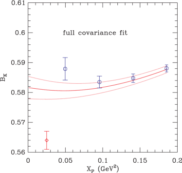
In Fig. 1(a), we show the fitting results with the full covariance matrix. As one can see, the fitting curve does not pass through the data points. The value is with degrees of freedom , which indicates that the fitting fails manifestly. Let us perform the eigenmode decomposition on and as follows:
| (12) |
where and are the eigenmode projection coefficients. As we can see in Table 1, the difference is for , and for , whereas it is only for . Hence, the procedure of the covariance fitting works hard for the coefficient of but works less precisely for the coefficients of and , mainly because the eigenvalue is significantly smaller than and . The irony is that the average data points, , has only overlap with while more than of them are dominated by and . As a result, the fitting function misses the average data points. In this sense, the failure of the full covariance fitting is obviously due to the fact that the covariance fitting tries to determine the coefficient of very precisely, while losing precisions in and direction. If the fitting function is exact, this procedure should yield a fitting result reasonably describing the data. However, if the fitting function has error in direction, this failing situation can happen.
| 1 | 2 | 3 | 4 | |
|---|---|---|---|---|
| 1.021(4) | 0.5655(14) | 0.1061(3) | 0.01442(3) | |
| 1.014(4) | 0.5679(11) | 0.1058(3) | 0.01443(3) |
3 Prescriptions for the trouble
If the covariance matrix has small eigenvalues, even a small error of fitting function may yield large error in fitting result. To circumvent this problem, we need some approximation methods, such as diagonal approximation or cutoff method. In subsection 3.1, we propose a new method which we call the eigenmode shift (ES) method.
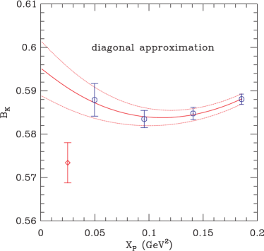
One simple solution to the problem is to use the diagonal approximation (uncorrelated fitting). In this method, we neglect the off-diagonal covariance as follows: In this way, the small eigenvalue problem disappears. The fitting results are shown in Fig. 1(b).
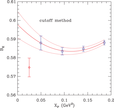
Another possible solution is to exclude the eigenmodes corresponding to the small eigenvalues from the inverse covariance matrix, . In our example, is removed by setting in Eq. (6). We call this the cutoff method. A number of lattice QCD groups [8, 9] use this method in the popular name of the SVD (singular value decomposition) method. In Fig. 2(a), we show the results of the covariance fitting using the cutoff method.


3.1 Eigenmode shift method
We know that the whole trouble comes from the error of fitting function in direction. Hence, we can think of a new fitting function defined as follows:
| (13) |
Here, is a tiny parameter that can be determined by the Bayesian method. Hence, we modify the as follows,
| (14) |
We know that is very tiny so we choose . As mentioned in section 2.2, the order of the neglected highest order term in the is . Hence, we set . Then we can do the full covariance fitting with an extra fitting parameter, . When we do the extrapolation to the physical pion mass, we use only the function, dropping out the terms. We call this the eigenmode shift (ES) method.
This is the same procedure as following: First, find a shifting vector, , which minimizes the . Then fit with the tuned(shifted) fitting function. To consider the statistical error of , do this procedure over jackknife or bootstrap samples.
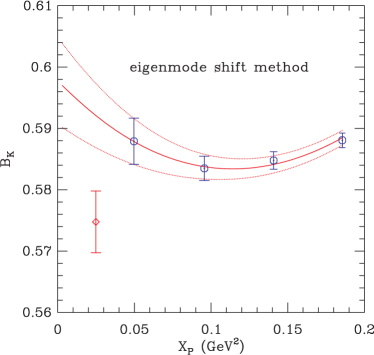
In our example, the fitted , which is much smaller by an order of magnitude than truncated highest order terms in . In Fig. 2(b), we show the fitting results obtained using the ES method. This method tunes the fitting function by a tiny amount so that minimizes the small eigenvalue contribution. In this sense, it looks similar to the cutoff method. However, unlike the cutoff method, the ES method determines the shifting parameter, , using the Bayesian method and the full covariance matrix remains untouched.
4 Conclusion
Here, we address an issue of covariance fitting on the highly correlated data. It turns out that the small error of fitting function can make the fitting fail if the covariance matrix has small eigenvalues. In order to get around the trouble, we have used approximations: the diagonal approximation and the cutoff method. Here, we propose a new method, the eigenmode shift method, which fine-tunes the fitting function, while keeping the covariance matrix untouched.
5 Acknowledgments
C. Jung is supported by the US DOE under contract DE-AC02-98CH10886. The research of W. Lee is supported by the Creative Research Initiatives Program (3348-20090015) of the NRF grant funded by the Korean government (MEST). W. Lee would like to acknowledge the support from KISTI supercomputing center through the strategic support program for the supercomputing application research [No. KSC-2011-C3-03]. Computations were carried out in part on QCDOC computing facilities of the USQCD Collaboration at Brookhaven National Lab, and on the DAVID GPU clusters at Seoul National University. The USQCD Collaboration are funded by the Office of Science of the U.S. Department of Energy.
References
- [1] T. Bae, et al., SWME Collaboration, Phys. Rev. D82, (2010), 114509 ; [arXiv:1008.5179].
- [2] Boram Yoon, et al., SWME Collaboration, [arXiv:1101.2248].
- [3] S. Gottlieb, et al., MILC Collaboration, Phys. Rev. D38, (1988), 2245.
- [4] D. Toussaint, From Action to Answers (World Scientific, 1990), 121.
- [5] T. Anderson, An Introduction to Multivariate Statistical Analysis (Wiley Interscience, 2003), 3rd ed.
- [6] R. Johnson and D. Wichern, Applied Multivariate Statistical Analysis (Pearson Prentice Hall, 2007), 6th ed.
- [7] M. Schervish, Theory of Statistics (Springer-Verlag, 1995).
- [8] J. Bailey, et al., PoS (LATTICE 2010) 306 ; [arXiv:1011.2423].
- [9] T. Bhattacharya, et al., Phys. Lett. B461, (1999), 79 ; [hep-lat/9904011].