Optimal and Approximate Q-value Functions
for Decentralized POMDPs

Abstract

Decision-theoretic planning is a popular approach to sequential decision making problems, because it treats uncertainty in sensing and acting in a principled way. In single-agent frameworks like MDPs and POMDPs, planning can be carried out by resorting to Q-value functions: an optimal Q-value function $Q^{*}$ is computed in a recursive manner by dynamic programming, and then an optimal policy is extracted from $Q^{*}$. In this paper we study whether similar Q-value functions can be defined for decentralized POMDP models (Dec-POMDPs), and how policies can be extracted from such value functions. We define two forms of the optimal Q-value function for Dec-POMDPs: one that gives a normative description as the Q-value function of an optimal pure joint policy and another one that is sequentially rational and thus gives a recipe for computation. This computation, however, is infeasible for all but the smallest problems. Therefore, we analyze various approximate Q-value functions that allow for efficient computation. We describe how they relate, and we prove that they all provide an upper bound to the optimal Q-value function $Q^{*}$. Finally, unifying some previous approaches for solving Dec-POMDPs, we describe a family of algorithms for extracting policies from such Q-value functions, and perform an experimental evaluation on existing test problems, including a new firefighting benchmark problem.

1 Introduction

One of the main goals in artificial intelligence (AI) is the development of intelligent agents, which perceive their environment through sensors and influence the environment through their actuators. In this setting, an essential problem is how an agent should decide which action to perform in a certain situation. In this work, we focus on planning: constructing a plan that specifies which action to take in each situation the agent might encounter over time. In particular, we will focus on planning in a cooperative multiagent system (MAS): an environment in which multiple agents coexist and interact in order to perform a joint task. We will adopt a decision-theoretic approach, which allows us to tackle uncertainty in sensing and acting in a principled way.

Decision-theoretic planning has roots in control theory and in operations research. In control theory, one or more controllers control a stochastic system with a specific output as goal. Operations research considers tasks related to scheduling, logistics and work flow and tries to optimize the concerning systems. Decision-theoretic planning problems can be formalized as Markov decision processes (MDPs), which have have been frequently employed in both control theory as well as operations research, but also have been adopted by AI for planning in stochastic environments. In all these fields the goal is to find a (conditional) plan, or policy, that is optimal with respect to the desired behavior. Traditionally, the main focus has been on systems with only one agent or controller, but in the last decade interest in systems with multiple agents or decentralized control has grown.

A different, but also related field is that of game theory. Game theory considers agents, called players, interacting in a dynamic, potentially stochastic process, the game. The goal here is to find optimal strategies for the agents, that specify how they should play and therefore correspond to policies. In contrast to decision-theoretic planning, game theory has always considered multiple agents, and as a consequence several ideas and concepts from game theory are now being applied in decentralized decision-theoretic planning. In this work we apply game-theoretic models to decision-theoretic planning for multiple agents.

1.1 Decision-Theoretic Planning

In the last decades, the Markov decision process (MDP) framework has gained in popularity in the AI community as a model for planning under uncertainty (?, ?). MDPs can be used to formalize a discrete time planning task of a single agent in a stochastically changing environment, on the condition that the agent can observe the state of the environment. Every time step the state changes stochastically, but the agent chooses an action that selects a particular transition function. Taking an action from a particular state at time step $t$ induces a probability distribution over states at time step $t+1$.

The agent’s objective can be formulated in several ways. The first type of objective of an agent is reaching a specific goal state, for example in a maze in which the agent’s goal is to reach the exit. A different formulation is given by associating a certain cost with the execution of a particular action in a particular state, in which case the goal will be to minimize the expected total cost. Alternatively, one can associate rewards with actions performed in a certain state, the goal being to maximize the total reward.

When the agent knows the probabilities of the state transitions, i.e., when it knows the model, it can contemplate the expected transitions over time and construct a plan that is most likely to reach a specific goal state, minimizes the expected costs or maximizes the expected reward. This stands in some contrast to reinforcement learning (RL) (?), where the agent does not have a model of the environment, but has to learn good behavior by repeatedly interacting with the environment. Reinforcement learning can be seen as the combined task of learning the model of the environment and planning, although in practice often it is not necessary to explicitly recover the environment model. In this article we focus only on planning, but consider two factors that complicate computing successful plans: the inability of the agent to observe the state of the environment as well as the presence of multiple agents.

In the real world an agent might not be able to determine what the state of the environment exactly is, because the agent’s sensors are noisy and/or limited. When sensors are noisy, an agent can receive faulty or inaccurate observations with some probability. When sensors are limited the agent is unable to observe the differences between states that cannot be detected by the sensor, e.g., the presence or absence of an object outside a laser range-finder’s field of view. When the same sensor reading might require different action choices, this phenomenon is referred to as perceptual aliasing. In order to deal with the introduced sensor uncertainty, a partially observable Markov decision process (POMDP) extends the MDP model by incorporating observations and their probability of occurrence conditional on the state of the environment (?).

The other complicating factor we consider is the presence of multiple agents. Instead of planning for a single agent we now plan for a team of cooperative agents. We assume that communication within the team is not possible. A major problem in this setting is how the agents will have to coordinate their actions. Especially, as the agents are not assumed to observe the state—each agent only knows its own observations received and actions taken—there is no common signal they can condition their actions on. Note that this problem is in addition to the problem of partial observability, and not a substitution of it; even if the agents could freely and instantaneously communicate their individual observations, the joint observations would not disambiguate the true state.

One option is to consider each agent separately, and have each such agent maintain an explicit model of the other agents. This is the approach as chosen in the Interactive POMDP (I-POMDP) framework (?). A problem in this approach, however, is that the other agents also model the considered agent, leading to an infinite recursion of beliefs regarding the behavior of agents. We will adopt the decentralized partially observable Markov decision process (Dec-POMDP) model for this class of problems (?). A Dec-POMDP is a generalization to multiple agents of a POMDP and can be used to model a team of cooperative agents that are situated in a stochastic, partially observable environment.

The single-agent MDP setting has received much attention, and many results are known. In particular it is known that an optimal plan, or policy, can be extracted from the optimal action-value, or Q-value, function $Q^{*}(s,a)$, and that the latter can be calculated efficiently. For POMDPs, similar results are available, although finding an optimal solution is harder (PSPACE-complete for finite-horizon problems, ?).

On the other hand, for Dec-POMDPs relatively little is known except that they are provably intractable (NEXP-complete, ?). In particular, an outstanding issue is whether Q-value functions can be defined for Dec-POMDPs just as in (PO)MDPs, and whether policies can be extracted from such Q-value functions. Currently most algorithms for planning in Dec-POMDPs are based on some version of policy search (?, ?, ?, ?), and a proper theory for Q-value functions in Dec-POMDPs is still lacking. Given the wide range of applications of value functions in single-agent decision-theoretic planning, we expect that such a theory for Dec-POMDPs can have great benefits, both in terms of providing insight as well as guiding the design of solution algorithms.

1.2 Contributions

In this paper we develop theory for Q-value functions in Dec-POMDPs, showing that an optimal Q-function $Q^{*}$ can be defined for a Dec-POMDP. We define two forms of the optimal Q-value function for Dec-POMDPs: one that gives a normative description as the Q-value function of an optimal pure joint policy and another one that is sequentially rational and thus gives a recipe for computation. We also show that given $Q^{*}$, an optimal policy can be computed by forward-sweep policy computation, solving a sequence of Bayesian games forward through time (i.e., from the first to the last time step), thereby extending the solution technique of ? (?) to the exact setting.

Computation of $Q^{*}$ is infeasible for all but the smallest problems. Therefore, we analyze three different approximate Q-value functions $\textrm{Q}_{\textrm{MDP}},$ $\textrm{Q}_{\textrm{POMDP}}$ and $\textrm{Q}_{\textrm{BG}}$ that can be more efficiently computed and which constitute upper bounds to $Q^{*}$. We also describe a generalized form of $\textrm{Q}_{\textrm{BG}}$ that includes $\textrm{Q}_{\textrm{POMDP}}$, $\textrm{Q}_{\textrm{BG}}$ and $Q^{*}$. This is used to prove a hierarchy of upper bounds: $Q^{*}\leq\textrm{Q}_{\textrm{BG}}\leq\textrm{Q}_{\textrm{POMDP}}\leq\textrm{Q}_{\textrm{MDP}}$.

Next, we show how these approximate Q-value functions can be used to compute optimal or sub-optimal policies. We describe a generic policy search algorithm, which we dub Generalized ${\textrm{MAA}^{*}}$ (${\textrm{GMAA}^{*}}$) as it is a generalization of the ${\textrm{MAA}^{*}}$ algorithm by ? (?), that can be used for extracting a policy from an approximate Q-value function. By varying the implementation of a sub-routine of this algorithm, this algorithm unifies ${\textrm{MAA}^{*}}$ and forward-sweep policy computation and thus the approach of ? (?).

Finally, in an experimental evaluation we examine the differences between $\textrm{Q}_{\textrm{MDP}}$, $\textrm{Q}_{\textrm{POMDP}}$, $\textrm{Q}_{\textrm{BG}}$ and $Q^{*}$ for several problems. We also experimentally verify the potential benefit of tighter heuristics, by testing different settings of ${\textrm{GMAA}^{*}}$ on some well known test problems and on a new benchmark problem involving firefighting agents.

This article is based on previous work by ? (?)—abbreviated OV here—containing several new contributions: (1) Contrary to the OV work, the current work includes a section on the sequential rational description of $Q^{*}$ and suggests a way to compute $Q^{*}$ in practice (OV only provided a normative description of $Q^{*}$). (2) The current work provides a formal proof of the hierarchy of upper bounds to $Q^{*}$ (which was only qualitatively argued in the OV paper). (3) The current article additionally contains a proof that the solutions for the Bayesian games with identical payoffs given by equation (4.2) constitute Pareto optimal Nash equilibria of the game (which was not proven in the OV paper). (4) This article contains a more extensive experimental evaluation of the derived bounds of $Q^{*}$, and introduces a new benchmark problem (firefighting). (5) Finally, the current article provides a more complete introduction to Dec-POMDPs and existing solution methods, as well as Bayesian games, hence it can serve as a self-contained introduction to Dec-POMDPs.

1.3 Applications

Although the field of multiagent systems in a stochastic, partially observable environment seems quite specialized and thus narrow, the application area is actually very broad. The real world is practically always partially observable due to sensor noise and perceptual aliasing. Also, in most of these domains communication is not free, but consumes resources and thus has a particular cost. Therefore models as Dec-POMDPs, which do consider partially observable environments are relevant for essentially all teams of embodied agents.

Example applications of this type are given by ? (?), who considered multi-robot navigation in which a team of agents with noisy sensors has to act to find/capture a goal. ? (?) use a multi-robot space exploration example. Here, the agents are Mars rovers and have to decide on how to proceed their mission: whether to collect particular samples at specific sites or not. The rewards of particular samples can be sub- or super-additive, making this task non-trivial. An overview of application areas in cooperative robotics is presented by ? (?), among which is robotic soccer, as applied in RoboCup (?). Another application that is investigated within this project is crisis management: RoboCup Rescue (?) models a situation where rescue teams have to perform a search and rescue task in a crisis situation. This task also has been modeled as a partially observable system (?, ?, ?, ?, ?).

There are also many other types of applications. ? (?, ?) give applications for distributed sensor networks (typically used for surveillance). An example of load balancing among queues is presented by ? (?). Here agents represent queues and can only observe queue sizes of themselves and immediate neighbors. They have to decide whether to accept new jobs or pass them to another queue. Another frequently considered application domain is communication networks. ? (?) treated a packet routing application in which agents are routers and have to minimize the average transfer time of packets. They are connected to immediate neighbors and have to decide at each time step to which neighbor to send each packet. Other approaches to communication networks using decentralized, stochastic, partially observable systems are given by ? (?, ?, ?).

1.4 Overview of Article

The rest of this article is organized as follows. In Section 2 we will first formally introduce the Dec-POMDP model and provide background on its components. Some existing solution methods are treated in Section 3. Then, in Section 4 we show how a Dec-POMDP can be modeled as a series of Bayesian games and how this constitutes a theory of Q-value functions for BGs. We also treat two forms of optimal Q-value functions, $Q^{*}$, here. Approximate Q-value functions are described in Section 5 and one of their applications is discussed in Section 6. Section 7 presents the results of the experimental evaluation. Finally, Section 8 concludes.

2 Decentralized POMDPs

In this section we define the Dec-POMDP model and discuss some of its properties. Intuitively, a Dec-POMDP models a number of agents that inhabit a particular environment, which is considered at discrete time steps, also referred to as stages (?) or (decision) epochs (?). The number of time steps the agents will interact with their environment is called the horizon of the decision problem, and will be denoted by $h$. In this paper the horizon is assumed to be finite. At each stage $t=0,1,2,\dots,h-1$ every agent takes an action and the combination of these actions influences the environment, causing a state transition. At the next time step, each agent first receives an observation of the environment, after which it has to take an action again. The probabilities of state transitions and observations are specified by the Dec-POMDP model, as are rewards received for particular actions in particular states. The transition- and observation probabilities specify the dynamics of the environment, while the rewards specify what behavior is desirable. Hence, the reward model defines the agents’ goal or task: the agents have to come up with a plan that maximizes the expected long term reward signal. In this work we assume that planning takes place off-line, after which the computed plans are distributed to the agents, who then merely execute the plans on-line. That is, computation of the plan is centralized, while execution is decentralized. In the centralized planning phase, the entire model as detailed below is available. During execution each agent only knows the joint policy as found by the planning phase and its individual history of actions and observations.

2.1 Formal Model

In this section we more formally treat the basic components of a Dec-POMDP. We start by giving a mathematical definition of these components.

Definition 2.1.

A decentralized partially observable Markov decision process (Dec-POMDP) is defined as a tuple $\left\langle n,\mathcal{S},\mathcal{A},T,R,\mathcal{O},O,h,b^{0}\right\rangle$ where:

• $n$ is the number of agents.

• $\mathcal{S}$ is a finite set of states.

• $\mathcal{A}$ is the set of joint actions.

• $T$ is the transition function.

• $R$ is the immediate reward function.

• $\mathcal{O}$ is the set of joint observations.

• $O$ is the observation function.

• $h$ is the horizon of the problem.

• $b^{0}\in\mathcal{P}(\mathcal{S})$, is the initial state distribution at time $t=0$.

The Dec-POMDP model extends single-agent (PO)MDP models by considering joint actions and observations. In particular, we define $\mathcal{A}=\times_{i}\mathcal{A}_{i}$ as the set of joint actions. Here, $\mathcal{A}_{i}$ is the set of actions available to agent $i$. Every time step, one joint action $a=\left\langle a_{1},...,a_{n}\right\rangle$ is taken. In a Dec-POMDP, agents only know their own individual action; they do not observe each other’s actions. We will assume that any action $a_{i}\in\mathcal{A}_{i}$ can be selected at any time. So the set $\mathcal{A}_{i}$ does not depend on the stage or state of the environment. In general, we will denote the stage using superscripts, so $a^{t}$ denotes the joint action taken at stage $t$, $a_{i}^{t}$ is the individual action of agent $i$ taken at stage $t$. Also, we write $a_{\neq i}=\left\langle a_{1},\dots,a_{i-1},a_{i+1},\dots,a_{n}\right\rangle$ for a profile of actions for all agents but $i$.

Similarly to the set of joint actions, $\mathcal{O}=\times_{i}\mathcal{O}_{i}$ is the set of joint observations, where $\mathcal{O}_{i}$ is a set of observations available to agent $i$. Every time step the environment emits one joint observation $o=\left\langle o_{1},...,o_{n}\right\rangle$, from which each agent $i$ only observes its own component $o_{i}$, as illustrated by Figure 1. Notation with respect to time and indices for observations is analogous to the notation for actions. In this paper, we will assume that the action- and observation sets are finite. Infinite action- and observation sets are very difficult to deal with even in the single-agent case, and to the authors’ knowledge no research has been performed on this topic in the partially observable, multiagent case.

Actions and observations are the interface between the agents and their environment. The Dec-POMDP framework describes this environment by its states and transitions. This means that rather than considering a complex, typically domain-dependent model of the environment that explains how this environment works, a descriptive stance is taken: A Dec-POMDP specifies an environment model simply as the set of states $\mathcal{S}=\left\{s_{1},...,s_{|\mathcal{S}|}\right\}$ the environment can be in, together with the probabilities of state transitions that are dependent on executed joint actions. In particular, the transition from some state to a next state depends stochastically on the past states and actions. This probabilistic dependence models outcome uncertainty: the fact that the outcome of an action cannot be predicted with full certainty.

An important characteristic of Dec-POMDPs is that the states possess the Markov property. That is, the probability of a particular next state depends on the current state and joint action, but not on the whole history:

$$P(s^{t+1}|s^{t},a^{t},s^{t-1},a^{t-1},...,s^{0},a^{0})=P(s^{t+1}|s^{t},a^{t}).$$ (2.1)

Also, we will assume that the transition probabilities are stationary, meaning that they are independent of the stage $t$.

In a way similar to how the transition model $T$ describes the stochastic influence of actions on the environment, the observation model $O$ describes how the state of the environment is perceived by the agents. Formally, $O$ is the observation function, a mapping from joint actions and successor states to probability distributions over joint observations: $O:\mathcal{A}\times\mathcal{S}\rightarrow\mathcal{P}(\mathcal{O})$. I.e., it specifies

$$P(o^{t}|a^{t-1},s^{t}).$$ (2.2)

This implies that the observation model also satisfies the Markov property (there is no dependence on the history). Also the observation model is assumed stationary: there is no dependence on the stage $t$.

\psfrag{decis}{\footnotesize actions}\psfrag{obs}{\footnotesize observations}\psfrag{states}{\footnotesize states}\psfrag{s0}[br][bc]{\footnotesize$s^{0}$}\psfrag{s1}[br][bc]{\footnotesize$s^{1}$}\psfrag{sh-1}[br][bc]{\footnotesize$s^{h-1}$}\psfrag{o0}[br][bc]{\footnotesize$o^{0}$}\psfrag{o1}[br][bc]{\footnotesize$o^{1}$}\psfrag{oh-1}[br][bc]{\footnotesize$o^{h-1}$}\psfrag{o0_1}[bc][bc]{\footnotesize$o_{1}^{0}$}\psfrag{o0_n}[br][bc]{\footnotesize$o_{n}^{0}$}\psfrag{o1_1}[bc][bc]{\footnotesize$o_{1}^{1}$}\psfrag{o1_n}[br][bc]{\footnotesize$o_{n}^{1}$}\psfrag{oh-1_1}[bc][bc]{\footnotesize$o_{1}^{h-1}$}\psfrag{oh-1_n}[br][bc]{\footnotesize$o_{n}^{h-1}$}\psfrag{a0}{\footnotesize$a^{0}$}\psfrag{a1}{\footnotesize$a^{1}$}\psfrag{ah-2}{\footnotesize$a^{h-2}$}\psfrag{ah-1}{\footnotesize$a^{h-1}$}\psfrag{vd}[Bl][Bc]{$\vdots$}\psfrag{...}[Bl][Bl]{$\dots$}\psfrag{a0_1}[Br][Bc]{\footnotesize$a_{1}^{0}$}\psfrag{a0_n}[Br][Bc]{\footnotesize$a_{n}^{0}$}\psfrag{a1_1}[Br][Bc]{\footnotesize$a_{1}^{1}$}\psfrag{a1_n}[Br][Bc]{\footnotesize$a_{n}^{1}$}\psfrag{ah-1_1}[Br][Bc]{\footnotesize$a_{1}^{h-1}$}\psfrag{ah-1_n}[Br][Bc]{\footnotesize$a_{n}^{h-1}$}\psfrag{ah-2}{\footnotesize$a^{h-2}$}\psfrag{ah-1}{\footnotesize$a^{h-1}$}\psfrag{ts}{\footnotesize$t$}\psfrag{t0}[br][bc]{\footnotesize$0$}\psfrag{t1}[br][bc]{\footnotesize$1$}\psfrag{th-1}[br][bc]{\footnotesize$h-1$}\psfrag{ttg}{\footnotesize$\tau$}\psfrag{ttg0}[cl][cl]{\footnotesize$h$}\psfrag{ttg1}[br][bc]{\footnotesize$h-1$}\psfrag{ttgh-1}[cl][cl]{\footnotesize$1$}\includegraphics[width=411.93767pt]{figs/process_history}

Figure 1: An illustration of the dynamics of a Dec-POMDP. At every stage the environment is in a particular state. This state emits a joint observation, of which each agent observes its individual observation. Then each agent selects an action forming the joint action.

Literature has identified different categories of observability (?, ?). When the observation function is such that the individual observation for all the agents will always uniquely identify the true state, the problem is considered fully- or individually observable. In such a case, a Dec-POMDP effectively reduces to a multiagent MDP (MMDP) as described by ? (?). The other extreme is when the problem is non-observable, meaning that none of the agents observes any useful information. This is modeled by the fact that agents always receive a null-observation, $\forall_{i}\;\mathcal{O}_{i}=\left\{o_{i,\emptyset}\right\}$. Under non-observability agents can only employ an open-loop plan. Between these two extremes there are partially observable problems. One more special case has been identified, namely the case where not the individual, but the joint observation identifies the true state. This case is referred to as jointly- or collectively observable. A jointly observable Dec-POMDP is referred to as a Dec-MDP.

The reward function $R(s,a)$ is used to specify the goal of the agents and is a function of states and joint actions. In particular, a desirable sequence of joint actions should correspond to a high ‘long-term’ reward, formalized as the return.

Definition 2.2.

Let the return or cumulative reward of a Dec-POMDP be defined as total of the rewards received during an execution:

$$r(0)+r(1)+\dots+r(h-1),$$ (2.3)

where $r(t)$ is the reward received at time step $t$.

When, at stage $t$, the state is $s^{t}$ and the taken joint action is $a^{t}$, we have that $r(t)=R(s^{t},a)$. Therefore, given the sequence of states and taken joint actions, it is straightforward to determine the return by substitution of $r(t)$ by $R(s^{t},a)$ in (2.3).

In this paper we consider as optimality criterion the expected cumulative reward, where the expectation refers to the expectation over sequences of states and executed joint actions. The planning problem is to find a conditional plan, or policy, for each agent to maximize the optimality criterion. In the Dec-POMDP case this amounts to finding a tuple of policies, called a joint policy that maximizes the expected cumulative reward.

Note that, in a Dec-POMDP, the agents are assumed not to observe the immediate rewards: observing the immediate rewards could convey information regarding the true state which is not present in the received observations, which is undesirable as all information available to the agents should be modeled in the observations. When planning for Dec-POMDPs the only thing that matters is the expectation of the cumulative future reward which is available in the off-line planning phase, not the actual reward obtained. Indeed, it is not even assumed that the actual reward can be observed at the end of the episode.

Summarizing, in this work we consider Dec-POMDPs with finite actions and observation sets and a finite planning horizon. Furthermore, we consider the general Dec-POMDP setting, without any simplifying assumptions on the observation, transition, or reward models.

2.2 Example: Decentralized Tiger Problem

Here we will describe the decentralized tiger problem introduced by ? (?). This test problem has been frequently used (?, ?, ?, ?) and is a modification of the (single-agent) tiger problem (?). It concerns two agents that are standing in a hallway with two doors. Behind one of the doors is a tiger, behind the other a treasure. Therefore there are two states: the tiger is behind the left door ($s_{l}$) or behind the right door ($s_{r}$). Both agents have 3 actions at their disposal: open the left door ($a_{\textrm{\tiny OL}}$), open the right door ($a_{\textrm{\tiny OR}}$) and listen ($a_{\textrm{\tiny Li}}$). But they cannot observe each other’s actions. In fact, they can only receive 2 observations. Either they hear a sound left ($o_{\textrm{\tiny HL}}$) or right ($o_{\textrm{\tiny HR}}$).

At $t=0$ the state is $s_{l}$ or $s_{r}$ with probability $0.5$. As long as no agent opens a door the state doesn’t change, when a door is opened, the state resets to $s_{l}$ or $s_{r}$ with probability $0.5$. The full transition, observation and reward model are listed by ? (?). The observation probabilities are independent, and identical for both agents. For instance, when the state is $s_{l}$ and both perform action $a_{\textrm{\tiny Li}}$, both agents have a 85% chance of observing $o_{\textrm{\tiny HL}}$, and the probability of both hearing the tiger left is $0.85\cdot 0.85=0.72$.

When the agents open the door for the treasure they receive a positive reward, while they receive a penalty for opening the wrong door. When opening the wrong door jointly, the penalty is less severe. Opening the correct door jointly leads to a higher reward.

Note that, when the wrong door is opened by one or both agents, they are attacked by the tiger and receive a penalty. However, neither of the agents observe this attack nor the penalty and the episode continues. Arguably, a more natural representation would be to have the episode end after a door is opened or to let the agents observe whether they encountered the tiger or treasure, however this is not considered in this test problem.

2.3 Histories

As mentioned, the goal of planning in a Dec-POMDP is to find a (near-) optimal tuple of policies, and these policies specify for each agent how to act in a specific situation. Therefore, before we define a policy, we first need to define exactly what these specific situations are. In essence such situations are those parts of the history of the process that the agents can observe.

Let us first consider what the history of the process is. A Dec-POMDP with horizon $h$ specifies $h$ time steps or stages $t=0,...,h-1$. At each of these stages, there is a state $s^{t}$, joint observation $o^{t}$ and joint action $a^{t}$. Therefore, when the agents will have to select their $k$-th actions (at $t=k-1$), the history of the process is a sequence of states, joint observations and joint actions, which has the following form:

$$\left(s^{0},o^{0},a^{0},s^{1},o^{1},a^{1},...,s^{k-1},o^{k-1}\right).$$

Here $s^{0}$ is the initial state, drawn according to the initial state distribution $b^{0}$. The initial joint observation $o^{0}$ is assumed to be the empty joint observation: $o^{0}=o_{\emptyset}=\left\langle o_{1,\emptyset},...,o_{n,\emptyset}\right\rangle$.

From this history of the process, the states remain unobserved and agent $i$ can only observe its own actions and observations. Therefore an agent will have to base its decision regarding which action to select on the sequence of actions and observations observed up to that point.

Definition 2.3.

We define the action-observation history for agent $i$, $\vec{\theta}_{i}$, as the sequence of actions taken by and observations received by agent $i$. At a specific time step $t$, this is:

$$\vec{\theta}_{i}^{\,t}=\left(o_{i}^{0},a_{i}^{0},o_{i}^{1}\dots,a_{i}^{t-1},o_{i}^{t}\right).$$

The joint action-observation history, $\vec{\theta},$ is the action-observation history for all agents:

$$\vec{\theta}{}^{\,t}=\langle\vec{\theta}_{1}^{\,t},\dots,\vec{\theta}_{n}^{\,t}\rangle.$$

Agent $i$’s set of possible action-observation histories at time $t$ is $\vec{\Theta}_{i}^{t}=\times_{t}(\mathcal{O}_{i}\times\mathcal{A}_{i})$. The set of all possible action-observation histories for agent $i$ is $\vec{\Theta}_{i}=\cup_{t=0}^{h-1}\vec{\Theta}_{i}^{t}$. Finally the set of all possible joint action-observation histories is given by $\vec{{\Theta}}=\cup_{t=0}^{h-1}(\vec{\Theta}_{1}^{t}\times...\times\vec{\Theta}_{n}^{t})$. At $t=0$, the action-observation history is empty, denoted by $\vec{\theta}{}^{\,0}=\vec{\theta}_{\emptyset}$.

We will also use a notion of history only using the observations of an agent.

Definition 2.4.

Formally, we define the observation history for agent $i$, $\vec{o}_{i}$, as the sequence of observations an agent has received. At a specific time step $t$, this is:

$$\vec{o}_{i}^{\,t}=\left(o_{i}^{0},o_{i}^{1},\dots,o_{i}^{t}\right).$$

The joint observation history, $\vec{o},$ is the observation history for all agents:

$$\vec{o}^{\,t}=\langle\vec{o}_{1}^{\,t},\dots,\vec{o}_{n}^{\,t}\rangle.$$

The set of observation histories for agent $i$ at time $t$ is denoted $\vec{\mathcal{O}}_{i}^{t}=\times_{t}\mathcal{O}_{i}$. Similar to the notation for action-observation histories, we also use $\vec{\mathcal{O}}_{i}$ and $\vec{\mathcal{O}}$ and the empty observation history is denoted $\vec{o}_{\emptyset}$.

Similarly we can define the action history as follows.

Definition 2.5.

The action history for agent $i$, $\vec{a}_{i}$, is the sequence of actions an agent has performed. At a specific time step $t$, we write:

$$\vec{a}_{i}^{\,t}=\left(a_{i}^{0},a_{i}^{1},\dots,a_{i}^{t-1}\right).$$

Notation for joint action histories and sets are analogous to those for observation histories. Also write $\vec{o}_{\neq i},\vec{\theta}_{\neq i},$ etc. to denote a tuple of observation-, action-observation histories, etc. for all agents except $i$. Finally we note that, clearly, an (joint) action-observation history consists of an (joint) action- and an (joint) observation history: $\vec{\theta}{}^{\,t}=\left\langle\vec{o}^{\,t},\vec{a}^{\,t}\right\rangle$.

2.4 Policies

As discussed in the previous section, the action-observation history of an agent specifies all the information the agent has when it has to decide upon an action. For the moment we assume that an individual policy $\pi_{i}$ for agent $i$ is a deterministic mapping from action-observation sequences to actions.

The number of possible action-observation histories is usually very large as this set grows exponentially with the horizon of the problem. At time step $t$, there are $\left(\left|\mathcal{A}_{i}\right|\cdot\left|\mathcal{O}_{i}\right|\right)^{t}$ action-observation histories for agent $i$. As a consequence there are a total of

$$\sum_{t=0}^{h-1}\left(\left|\mathcal{A}_{i}\right|\cdot\left|\mathcal{O}_{i}\right|\right)^{t}=\frac{\left(\left|\mathcal{A}_{i}\right|\cdot\left|\mathcal{O}_{i}\right|\right)^{h}-1}{\left(\left|\mathcal{A}_{i}\right|\cdot\left|\mathcal{O}_{i}\right|\right)-1}$$

of such sequences for agent $i$. Therefore the number of policies for agent $i$ becomes:

$$\left|\mathcal{A}_{i}\right|^{\frac{\left(\left|\mathcal{A}_{i}\right|\cdot\left|\mathcal{O}_{i}\right|\right)^{h}-1}{\left(\left|\mathcal{A}_{i}\right|\cdot\left|\mathcal{O}_{i}\right|\right)-1}},$$ (2.4)

which is doubly exponential in the horizon $h$.

2.4.1 Pure and Stochastic Policies

\psfrag{a1}[ct][cc]{\small$a_{\textrm{\tiny OL}}$}\psfrag{a2}[ct][cc]{\small$a_{\textrm{\tiny Li}}$}\psfrag{a3}[ct][cc]{\small$a_{\textrm{\tiny OR}}$}\psfrag{o1}[cc][cc]{\small$o_{\textrm{\tiny HL}}$}\psfrag{o2}[cc][cc]{\small$o_{\textrm{\tiny HR}}$}\psfrag{aoh}[lt][lc]{\small act.-obs. history}\includegraphics[width=433.62pt]{figs/Policy_tree-deterministic}

Figure 2: A deterministic policy can be represented as a tree. Left: a tree of action-observation histories $\vec{\theta}_{i}$ for one of the agents from the Dec-Tiger problem. An arbitrary deterministic policy $\pi_{i}$ is highlighted. Clearly shown is that $\pi_{i}$ only reaches a subset of of histories $\vec{\theta}_{i}$. ($\vec{\theta}_{i}$ that are not reached are not further expanded.) Right: The same policy can be shown in a simplified policy tree.

It is possible to reduce the number of policies under consideration by realizing that a lot of policies specify the same behavior. This is illustrated by the left side of Figure 2, which clearly shows that under a deterministic policy only a subset of possible action-observation histories are reached. Policies that only differ with respect to an action-observation history that is not reached in the first place, manifest the same behavior. The consequence is that in order to specify a deterministic policy, the observation history suffices: when an agent takes its action deterministically, he will be able to infer what action he took from only the observation history as illustrated by the right side of Figure 2.

Definition 2.6.

A pure or deterministic policy, $\pi_{i}$, for agent $i$ in a Dec-POMDP is a mapping from observation histories to actions, $\pi_{i}:\vec{\mathcal{O}}_{i}\rightarrow\mathcal{A}_{i}$. The set of pure policies of agent $i$ is denoted $\Pi_{i}$.

Note that also for pure policies we sometimes write $\pi_{i}(\vec{\theta}_{i})$. In this case we mean the action that $\pi_{i}$ specifies for the observation history contained in $\vec{\theta}_{i}$. For instance, let $\vec{\theta}_{i}=\left\langle\vec{o}_{i},\vec{a}_{i}\right\rangle$, then $\pi_{i}(\vec{\theta}_{i})=\pi_{i}(\vec{o}_{i})$. We use $\pi=\left\langle\pi_{1},...,\pi_{n}\right\rangle$ to denote a joint policy, a profile specifying a policy for each agent. We say that a pure joint policy is an induced or implicit mapping from joint observation histories to joint actions $\pi:\vec{\mathcal{O}}\rightarrow\mathcal{A}$. That is, the mapping is induced by individual policies $\pi_{i}$ that make up the joint policy. Also we use $\pi_{\neq i}=\left\langle\pi_{1},\dots,\pi_{i-1},\pi_{i+1},\dots,\pi_{n}\right\rangle$, to denote a profile of policies for all agents but $i$.

Apart from pure policies, it is also possible to have the agents execute randomized policies, i.e., policies that do not always specify the same action for the same situation, but in which there is an element of chance that decides which action is performed. There are two types of randomized policies: mixed policies and stochastic policies.

Definition 2.7.

A mixed policy, $\mu_{i}$, for an agent $i$ is a set of pure policies, $\mathcal{M}\subseteq\Pi_{i}$, along with a probability distribution over this set. Thus a mixed policy $\mu_{i}\in\mathcal{P}(\mathcal{M})$ is an element of the set of probability distributions over $\mathcal{M}$.

Definition 2.8.

A stochastic or behavioral policy, $\varsigma_{i}$, for agent $i$ is a mapping from action-observation histories to probability distributions over actions, $\varsigma_{i}:\vec{\Theta}_{i}\rightarrow\mathcal{P}(\mathcal{A}_{i})$.

When considering stochastic policies, keeping track of only the observations is insufficient, as in general all action-observation histories can be realized. That is why stochastic policies are defined as a mapping from the full space of action-observation histories to probability distributions over actions. Note that we use $\pi_{i}$ and $\Pi_{i}$ to denote a policy (space) in general, so also for randomized policies. We will only use $\pi_{i}$, $\mu_{i}$ and $\varsigma_{i}$ when there is a need to discriminate between different types of policies.

A common way to represent the temporal structure in a policy is to split it in decision rules $\delta_{i}$ that specify the policy for each stage. An individual policy is then represented as a sequence of decision rules $\pi_{i}=(\delta_{i}^{0},\dots,\delta_{i}^{h-1})$. In case of a deterministic policy, the form of the decision rule for stage $t$ is a mapping from length-$t$ observation histories to actions $\delta_{i}^{t}:\vec{\mathcal{O}}_{i}^{t}\rightarrow\mathcal{A}_{i}$.

2.4.2 Special Cases with Simpler Policies.

There are some special cases of Dec-POMDPs in which the policy can be specified in a simpler way. Here we will treat three such cases: in case the state $s$ is observable, in the single-agent case and the case that combines the previous two: a single agent in an environment of which it can observe the state.

The last case, a single agent in a fully observable environment, corresponds to the regular MDP setting. Because the agent can observe the state, which is Markovian, the agent does not need to remember any history, but can simply specify the decision rules $\delta$ of its policy $\pi=\left(\delta^{0},\dots,\delta^{h-1}\right)$ as mappings from states to actions: $\forall t\;\delta^{t}:\mathcal{S}\rightarrow\mathcal{A}$. The complexity of the policy representation reduces even further in the infinite-horizon case, where an optimal policy $\pi^{*}$ is known to be stationary. As such, there is only one decision rule $\delta$, that is used for all stages.

The same is true for multiple agents that can observe the state, i.e., a fully observable Dec-POMDP as defined in Section 2.1. This is essentially the same setting as the multiagent Markov decision process (MMDP) introduced by ? (?). In this case, the decision rules for agent $i$’s policy are mappings from states to actions $\forall t\;\delta_{i}^{t}:\mathcal{S}\rightarrow\mathcal{A}_{i}$, although in this case some care needs to be taken to make sure no coordination errors occur when searching for these individual policies.

In a POMDP, a Dec-POMDP with a single agent, the agent cannot observe the state, so it is not possible to specify a policy as a mapping from states to actions. However, it turns out that maintaining a probability distribution over states, called belief, $b\in\mathcal{P}(\mathcal{S})$, is a Markovian signal:

$$P(s^{t+1}|a^{t},o^{t},a^{t-1},o^{t-1},\dots,a^{0},o^{0})=P(s^{t+1}|b^{t},a^{t}),$$

where the belief $b^{t}$ is defined as

$$\forall_{s^{t}}\quad b^{t}(s^{t})\ \operatorname{\equiv}\ P(s^{t}|o^{t},a^{t-1},o^{t-1},\dots,a^{0},o^{0})=P(s^{t}|b^{t-1},a^{t-1},o^{t}).$$

As a result, a single agent in a partially observable environment can specify its policy as a series of mappings from the set of beliefs to actions $\forall t\;\delta^{t}:\mathcal{P}(\mathcal{S})\rightarrow\mathcal{A}$.

Unfortunately, in the general case we consider, no such space-saving simplifications of the policy are possible. Even though the transition and observation model can be used to compute a joint belief, this computation requires knowledge of the joint actions and observations. During execution, the agents simply have no access to this information and thus can not compute a joint belief.

2.4.3 The Quality of Joint Policies

Clearly, policies differ in how much reward they can expect to accumulate, which will serve as a criterion of a joint policy’s quality. Formally, we consider the expected cumulative reward of a joint policy, also referred to as its value.

Definition 2.9.

The value $V(\pi)$ of a joint policy $\pi$ is defined as

$$V(\pi)\ \operatorname{\equiv}\ E\Bigl{[}\sum_{t=0}^{h-1}R(s^{t},a^{t})\Big{|}\pi,b^{0}\Bigr{]},$$ (2.5)

where the expectation is over states, observations and—in the case of a randomized $\pi$—actions.

In particular we can calculate this expectation as

$$V(\pi)=\sum_{t=0}^{h-1}\sum_{\vec{\theta}{}^{\,t}\in\vec{{\Theta}}{}^{t}}\sum_{s^{t}\in\mathcal{S}}P(s^{t},\vec{\theta}{}^{\,t}|\pi,b^{0})\sum_{a^{t}\in\mathcal{A}}R(s^{t},a^{t})P_{\pi}(a^{t}|\vec{\theta}{}^{\,t}),$$ (2.6)

where $P_{\pi}(a^{t}|\vec{\theta}{}^{\,t})$ is the probability of $a$ as specified by $\pi$, and where $P(s^{t},\vec{\theta}{}^{\,t}|\pi,b^{0})$ is recursively defined as

$$P(s^{t},\vec{\theta}{}^{\,t}|\pi,b^{0})=\sum_{s^{t-1}\in\mathcal{S}}P(s^{t},\vec{\theta}{}^{\,t}|s^{t-1},\vec{\theta}{}^{\,t-1},\pi)P(s^{t-1},\vec{\theta}{}^{\,t-1}|\pi,b^{0}),$$ (2.7)

with

$$P(s^{t},\vec{\theta}{}^{\,t}|s^{t-1},\vec{\theta}{}^{\,t-1},\pi)=P(o^{t}|a^{t-1},s^{t})P(s^{t}|s^{t-1},a^{t-1})P_{\pi}(a^{t-1}|\vec{\theta}{}^{\,t-1})$$ (2.8)

a term that is completely specified by the transition and observation model and the joint policy. For stage $0$ we have that $P(s^{0},\vec{\theta}_{\emptyset}|\pi,b^{0})=b^{0}(s^{0})$.

Because of the recursive nature of $P(s^{t},\vec{\theta}{}^{\,t}|\pi,b^{0})$ it is more intuitive to specify the value recursively:

$$V_{\pi}(s^{t},\vec{\theta}{}^{\,t})=\sum_{a^{t}\in\mathcal{A}}P_{\pi}(a^{t}|\vec{\theta}{}^{\,t})\left[R(s^{t},a^{t})+\sum_{s^{t+1}\in\mathcal{S}}\sum_{o^{t+1}\in\mathcal{O}}P(s^{t+1},o^{t+1}|s^{t},a^{t})V_{\pi}(s^{t+1},\vec{\theta}{}^{\,t+1})\right],$$ (2.9)

with $\vec{\theta}{}^{\,t+1}=(\vec{\theta}{}^{\,t},a^{t},o^{t+1})$. The value of joint policy $\pi$ is then given by

$$V(\pi)=\sum_{s^{0}\in\mathcal{S}}V_{\pi}(s^{0},\vec{\theta}_{\emptyset})b^{0}(s^{0}).$$ (2.10)

For the special case of evaluating a pure joint policy $\pi$, eq. (2.6) can be written as:

$$V(\pi)=\sum_{t=0}^{h-1}\sum_{\vec{\theta}{}^{\,t}\in\vec{{\Theta}}{}^{t}}P(\vec{\theta}{}^{\,t}|\pi,b^{0})R(\vec{\theta}{}^{\,t},\pi(\vec{\theta}{}^{\,t})),$$ (2.11)

where

$$R(\vec{\theta}{}^{\,t},a^{t})=\sum_{s^{t}\in\mathcal{S}}R(s^{t},a^{t})P(s^{t}|\vec{\theta}{}^{\,t},b^{0})$$ (2.12)

denotes the expected immediate reward. In this case, the recursive formulation (2.9) reduces to

$$V_{\pi}^{t}(s^{t},\vec{o}^{\,t})=R\left(s^{t},\pi(\vec{o}^{\,t})\right)+\sum_{s^{t+1}\in\mathcal{S}}\sum_{o^{t+1}\in\mathcal{O}}P(s^{t+1},o^{t+1}|s^{t},\pi(\vec{o}^{\,t}))V_{\pi}^{t+1}(s^{t+1},\vec{o}^{\,t+1}).$$ (2.13)

Note that, when performing the computation of the value for a joint policy recursively, intermediate results should be cached. A particular $(s^{t+1},\vec{o}^{\,t+1})$-pair (or $(s^{t+1},\vec{\theta}{}^{\,t+1})$-pair for a stochastic joint policy) can be reached from $\left|\mathcal{S}\right|$ states $s^{t}$ of the previous stage. The value $V_{\pi}^{t+1}(s^{t+1},\vec{o}^{\,t+1})$ is the same, however, and should be computed only once.

2.4.4 Existence of an Optimal Pure Joint Policy

Although randomized policies may be useful, we can restrict our attention to pure policies without sacrificing optimality, as shown by the following.

Proposition 2.1.

A Dec-POMDP has at least one optimal pure joint policy.

Proof.

See appendix A.1.∎

3 Overview of Dec-POMDP Solution Methods

In order to provide some background on solving Dec-POMDPs, this section gives an overview of some recently proposed methods. We will limit this review to a number of finite-horizon methods for general Dec-POMDPs that are related to our own approach.

We will not review the work performed on infinite-horizon Dec-POMDPs, such as the work by ? (?, ?, ?, ?, ?). In this setting policies are usually represented by finite state controllers (FSCs). Since an infinite-horizon Dec-POMDP is undecidable (?), this line of work, focuses on finding $\epsilon$-approximate solutions (?) or (near-) optimal policies for given a particular controller size.

There also is a substantial amount of work on methods exploiting particular independence assumptions. In particular, transition and observation independent Dec-MDPs (?, ?) and Dec-POMDPs (?, ?) have received quite some attention. These models assume that each agent $i$ has an individual state space $\mathcal{S}_{i}$ and that the actions of one agent do not influence the transitions between the local states of another agent. Although such models are easier to solve, the independence assumptions severely restrict their applicability. Other special cases that have been considered are, for instance, goal oriented Dec-POMDPs (?), event-driven Dec-MDPs (?), Dec-MDPs with time and resource constraints (?, ?, ?), Dec-MDPs with local interactions (?) and factored Dec-POMDPs with additive rewards (?).

A final body of related work which is beyond the scope of this article are models and techniques for explicit communication in Dec-POMDP settings (?, ?, ?, ?, ?, ?, ?, ?, ?). The Dec-POMDP model itself can model communication actions as regular actions, in which case the semantics of the communication actions becomes part of the optimization problem (?, ?, ?). In contrast, most approaches mentioned typically assume that communication happens outside the Dec-POMDP model and with pre-defined semantics. A typical assumption is that at every time step the agents communicate their individual observations before selecting an action. ? (?) showed that, under assumptions of instantaneous and cost-free communication, sharing individual observations in such a way is optimal.

3.1 Brute Force Policy Evaluation

Because there exists an optimal pure joint policy for a finite-horizon Dec-POMDP, it is in theory possible to enumerate all different pure joint policies, evaluate them using equations (2.10) and (2.13) and choose the best one. The number of pure joint policies to be evaluated is:

$$O\left(|\mathcal{A}_{*}|^{\frac{n(|\mathcal{O}_{*}|^{h}-1)}{|\mathcal{O}_{*}|-1}}\right),$$ (3.1)

where $|\mathcal{A}_{*}|$ and $|\mathcal{O}_{*}|$ denote the largest individual action and observation sets. The cost of evaluating each policy is $O\left(|\mathcal{S}|\cdot|\mathcal{O}|^{h}\right)$. The resulting total cost of brute-force policy evaluation is

$$O\left(|\mathcal{A}_{*}|^{\frac{n(|\mathcal{O}_{*}|^{h}-1)}{|\mathcal{O}_{*}|-1}}\times|\mathcal{S}|\times|\mathcal{O}_{*}|^{nh}\right),$$ (3.2)

which is doubly exponential in the horizon $h$.

3.2 Alternating Maximization

? (?) introduced Joint Equilibrium based Search for Policies (JESP). This method guarantees to find a locally optimal joint policy, more specifically, a Nash equilibrium: a tuple of policies such that for each agent $i$ its policy $\pi_{i}$ is a best response for the policies employed by the other agents $\pi_{\neq i}$. It relies on a process we refer to as alternating maximization. This is a procedure that computes a policy $\pi_{i}$ for an agent $i$ that maximizes the joint reward, while keeping the policies of the other agents fixed. Next, another agent is chosen to maximize the joint reward by finding its best-response to the fixed policies of the other agents. This process is repeated until the joint policy converges to a Nash equilibrium, which is a local optimum. The main idea of fixing some agents and having others improve their policy was presented before by ? (?), but they used a heuristic approach for memory-less agents. The process of alternating maximization is also referred to as hill-climbing or coordinate ascent.

? (?) describe two variants of JESP, the first of which, Exhaustive-JESP, implements the above idea in a very straightforward fashion: Starting from a random joint policy, the first agent is chosen. This agent then selects its best-response policy by evaluating the joint reward obtained for all of its individual policies when the other agents follow their fixed policy.

The second variant, DP-JESP, uses a dynamic programming approach to compute the best-response policy for a selected agent $i$. In essence, fixing the policies of all other agents allows for a reformulation of the problem as an augmented POMDP. In this augmented POMDP a state $\bar{s}=\langle s,\vec{o}_{\neq i}^{\,}\rangle$ consists of a nominal state $s$ and the observation histories of the other agents $\vec{o}_{\neq i}^{\,}$. Given the fixed deterministic policies of other agents $\pi_{\neq i}$, such an augmented state $\bar{s}$ is a Markovian state, and all transition and observation probabilities can easily be derived from $\pi_{\neq i}$.

Like most methods proposed for Dec-POMDPs, JESP exploits the knowledge of the initial belief $b^{0}$ by only considering reachable beliefs $b(\bar{s})$ in the solution of the POMDP. However, in some cases the initial belief might not be available. As demonstrated by ? (?), JESP can be extended to plan for the entire space of initial beliefs, overcoming this problem.

3.3 ${\textrm{MAA}^{*}}$

? (?) introduced a heuristically guided policy search method called multiagent A* (${\textrm{MAA}^{*}}$). It performs a guided A*-like search over partially specified joint policies, pruning joint policies that are guaranteed to be worse than the best (fully specified) joint policy found so far by an admissible heuristic.

In particular ${\textrm{MAA}^{*}}$ considers joint policies that are partially specified with respect to time: a partial joint policy $\varphi^{t}=(\delta^{0},\delta^{1},\dots,\delta^{t-1})$ specifies the joint decision rules for the first $t$ stages. For such a partial joint policy $\varphi^{t}$ a heuristic value $\widehat{V}(\varphi^{t})$ is calculated by taking $V^{0\dots t-1}(\varphi^{t})$, the actual expected reward $\varphi^{t}$ achieves over the first $t$ stages, and adding $\widehat{V}^{t\dots h-1}$, a heuristic value for the remaining $h-t$ stages. Clearly when $\widehat{V}^{t\dots h-1}$ is an admissible heuristic—a guaranteed overestimation—so is $\widehat{V}(\varphi^{t})$.

${\textrm{MAA}^{*}}$ starts by placing the completely unspecified joint policy $\varphi^{0}$ in an open list. Then, it proceeds by selecting partial joint policies $\varphi^{t}=(\delta^{0},\delta^{1},\dots,\delta^{t-1})$ from the list and ‘expanding’ them: generating all $\varphi^{t+1}=(\delta^{0},\delta^{1},\dots,\delta^{t-1},\delta^{t})$ by appending all possible joint decision rules $\delta^{t}$ for next time step ($t)$. The left side of Figure (3) illustrates the expansion process. After expansion, all created children are heuristically valuated and placed in the open list, any partial joint policies $\varphi^{t+1}$ with $\widehat{V}(\varphi^{t+1})$ less than the expected value $V(\pi)$ of some earlier found (fully specified) joint policy $\pi$, can be pruned. The search ends when the list becomes empty, at which point we have found an optimal fully specified joint policy.

3.4 Dynamic Programming for Dec-POMDPs

\psfrag{a1}[cc][cc]{\normalsize$a$}\psfrag{a2}[cc][cc]{\normalsize$\bar{a}$}\psfrag{o1}[cc][cc]{\normalsize$o$}\psfrag{o2}[cc][cc]{\normalsize$\bar{o}$}\psfrag{old}{\normalsize`old' component}\psfrag{new}{\normalsize`new' component}\includegraphics[width=346.89731pt]{figs/policy_tree_construction-MAAvsJESP_d}

Figure 3: Difference between policy construction in ${\textrm{MAA}^{*}}$ (left) and dynamic programming (right) for an agent with actions $a,\bar{a}$ and observations $o,\bar{o}$. The dashed components are newly generated, dotted components result from the previous iteration. ${\textrm{MAA}^{*}}$ ‘expands’ a partial policy from the leaves, while dynamic programming backs up a set of ‘sub-tree policies’ forming new ones.

${\textrm{MAA}^{*}}$ incrementally builds policies from the first stage $t=0$ to the last $t=h-1$. Prior to this work, ? (?) introduced dynamic programming (DP) for Dec-POMDPs, which constructs policies the other way around: starting with a set of ‘1-step policies’ (actions) that can be executed at the last stage, they construct a set of 2-step policies to be executed at $h-2$, etc.

It should be stressed that the policies maintained are quite different from those used by ${\textrm{MAA}^{*}}$. In particular a partial policy in ${\textrm{MAA}^{*}}$ has the form $\varphi^{t}=(\delta^{0},\delta^{1},\dots,\delta^{t-1})$. The policies maintained by DP do not have such a correspondence to decision rules. We define the time-to-go $\tau$ at stage $t$ as

$$\tau=h-t.$$ (3.3)

Now $q_{i}^{\tau=k}$ denotes a $k$-steps-to-go sub-tree policy for agent $i$. That is, $q_{i}^{\tau=k}$ is a policy tree that has the same form as a full policy for the horizon-$k$ problem. Within the original horizon-$h$ problem $q_{i}^{\tau=k}$ is a candidate for execution starting at stage $t=h-k$. The set of $k$-steps-to-go sub-tree policies maintained for agent $i$ is denoted $\mathcal{Q}_{i}^{\tau=k}.$ Dynamic programming for Dec-POMDPs is based on backup operations: constructing $\mathcal{Q}_{i}^{\tau=k+1}$ a set of sub-tree policies $q_{i}^{\tau=k+1}$ from a set $\mathcal{Q}_{i}^{\tau=k}$. For instance, the right side of Figure 3 shows how $q_{i}^{\tau=3}$, a 3-steps-to-go sub-tree policy, is constructed from two $q_{i}^{\tau=2}\in\mathcal{Q}_{i}^{\tau=2}$. Also illustrated is the difference between this process and ${\textrm{MAA}^{*}}$ expansion (on the left side).

Dynamic programming consecutively constructs $\mathcal{Q}_{i}^{\tau=1},\mathcal{Q}_{i}^{\tau=2},\dots,\mathcal{Q}_{i}^{\tau=h}$ for all agents $i$. However, the size of the set $\mathcal{Q}_{i}^{\tau=k+1}$ is given by

$$|\mathcal{Q}_{i}^{\tau=k+1}|=\left|\mathcal{A}_{i}\right||\mathcal{Q}_{i}^{\tau=k}|^{\left|\mathcal{O}_{i}\right|},$$

and as a result the sizes of the maintained sets grow doubly exponential with $k$. To counter this source of intractability, ? (?) propose to eliminate dominated sub-tree policies. The expected reward of a particular sub-tree policy $q_{i}^{\tau=k}$ depends on the probability over states when $q_{i}^{\tau=k}$ is started (at stage $t=h-k$) as well as the probability with which the other agents $j\neq i$ select their sub-tree policies $q_{j}^{\tau=k}\in\mathcal{Q}_{j}^{\tau=k}$. If we let $q_{\neq i}^{\tau=k}$ denote a sub-tree profile for all agents but $i$, and $\mathcal{Q}_{\neq i}^{\tau=k}$ the set of such profiles, we can say that $q_{i}^{\tau=k}$ is dominated if it is not maximizing at any point in the multiagent belief space: the simplex over $S\times\mathcal{Q}_{\neq i}^{\tau=k}$. ? test for dominance over the entire multiagent belief space by linear programming. Removal of a dominated sub-tree policy $q_{i}^{\tau=k}$ of an agent $i$ may cause a sub-tree policy $q_{j}^{\tau=k}$ of an other agent $j$ to become dominated. Therefore ? propose to iterate over agents until no further pruning is possible, a procedure known as iterated elimination of dominated policies (?).

Finally, when the last backup step is completed the optimal policy can be found by evaluating all joint policies $\pi\in\mathcal{Q}_{1}^{\tau=h}\times\dots\times\mathcal{Q}_{n}^{\tau=h}$ for the initial belief $b^{0}$.

3.5 Extensions on DP for Dec-POMDPs

In the last few years several extensions to the dynamic programming algorithm for Dec-POMDPs have been proposed. The first of these extensions is due to ? (?). Rather than testing for dominance over the entire multiagent belief space, ? propose to perform point-based dynamic programming (PBDP). In order to prune the set of sub-tree policies $\mathcal{Q}_{i}^{\tau=k}$, the set of all the belief points $\mathcal{B}_{i,\textrm{reachable}}\subset\mathcal{P}(S\times\mathcal{Q}_{\neq i}^{\tau=k})$ that can possibly be reached by deterministic joint policies are generated. Only the sub-tree policies $q_{i}^{\tau=k}$ that maximize the value at some $b_{i}\in\mathcal{B}_{i,\textrm{reachable}}$ are kept. The proposed algorithm is optimal, but intractable because it needs to generate all the multiagent belief points that are reachable through all joint policies. To overcome this bottleneck, ? propose to randomly sample one or more joint policies and use those to generate $\mathcal{B}_{i,\textrm{reachable}}$.

? (?) also proposed a point-based extension of the DP algorithm, called memory-bounded dynamic programming (MBDP). Rather than using a randomly selected policy to generate the belief points, they propose to use heuristic policies. A more important difference, however, lies in the pruning step. Rather than pruning dominated sub-tree policies $q_{i}^{\tau=k}$, MBDP prunes all sub-tree policies except a few in each iteration. More specifically, for each agent maxTrees sub-tree policies are retained, which is a parameter of the planning method. As a result, MBDP has only linear space and time complexity with respect to the horizon. The MBDP algorithm still depends on the exhaustive generation of the sets $\mathcal{Q}_{i}^{\tau=k+1}$ which now contain $\left|\mathcal{A}_{i}\right|maxTrees^{\left|\mathcal{O}_{i}\right|}$ sub-tree policies. Moreover, in each iteration all $\left(\left|\mathcal{A}_{*}\right|maxTrees^{\left|\mathcal{O}_{*}\right|}\right)^{n}$ joint sub-tree policies have to be evaluated for each of the sampled belief points. To counter this growth, ? (?) proposed an extension that limits the considered observations during the backup step to the maxObs most likely observations.

Finally, a further extension of the DP for Dec-POMDPs algorithm is given by ? (?). Their approach, bounded DP (BDP), establishes a bound not on the used memory, but on the quality of approximation. In particular, BDP uses $\epsilon$-pruning in each iteration. That is, a $q_{i}^{\tau=k}$ that is maximizing in some region of the multiagent belief space, but improves the value in this region by at most $\epsilon$, is also pruned. Because iterated elimination using $\epsilon$- pruning can still lead to an unbounded reduction in value, ? propose to perform one iteration of $\epsilon$-pruning, followed by iterated elimination using normal pruning.

3.6 Other Approaches for Finite-Horizon Dec-POMDPs

There are a few other approaches for finite-horizon Dec-POMDPs, which we will only briefly describe here. ? (?) proposed a mixed integer linear programming formulation for the optimal solution of finite-horizon Dec-POMDPs. Their approach is based on representing the set of possible policies for each agent in sequence form (?, ?, ?). In sequence form, a single policy for an agent $i$ is represented as a subset of the set of ‘sequences’ (roughly corresponding to action-observation histories) for the agent. As such the problem can be interpreted as a combinatorial optimization problem, which ? propose to solve with a mixed integer linear program.

? (?) also recognize that finding a solution for Dec-POMDPs in essence is a combinatorial optimization problem and propose to apply the Cross-Entropy method (?), a method for combinatorial optimization that recently has become popular because of its ability to find near-optimal solutions in large optimization problems. The resulting algorithm performs a sampling-based policy search for approximately solving Dec-POMDPs. It operates by sampling pure policies from an appropriately parameterized stochastic policy, and then evaluates these policies either exactly or approximately in order to define the next stochastic policy to sample from, and so on until convergence.

Finally, ? (?, ?) proposed to approximate Dec-POMDPs through series of Bayesian games. Since our work in this article is based on the same representation, we defer a detailed explanation to the next section. We do mention here that while ? assume that the algorithm is run on-line (interleaving planning and execution), no such assumption is necessary. Rather we will apply the same framework during a off-line planning phase, just like the other algorithms covered in this overview.

4 Optimal Q-value Functions

In this section we will show how a Dec-POMDP can be modeled as a series of Bayesian games (BGs). A BG is a game-theoretic model that can deal with uncertainty (?). Bayesian games are similar to the more well-known normal form, or matrix games, but allow to model agents that have some private information. This section will introduce Bayesian games and show how a Dec-POMDP can be modeled as a series of Bayesian games (BGs). This idea of using a series of BGs to find policies for a Dec-POMDP has been proposed in an approximate setting by ? (?). In particular, they showed that using series of BGs and an approximate payoff function, they were able to obtain approximate solutions on the Dec-Tiger problem, comparable to results for JESP (see Section 3.2).

The main result of this section is that an optimal Dec-POMDP policy can be computed from the solution of a sequence of Bayesian games, if the payoff function of those games coincides with the Q-value function of an optimal policy $\pi^{*}$, i.e., with the optimal Q-value function $Q^{*}$. Thus, we extend the results of ? (?) to include the optimal setting. Also, we conjecture that this form of $Q^{*}$ can not be computed without already knowing an optimal policy $\pi^{*}$. By transferring the game-theoretic concept of sequential rationality to Dec-POMDPs, we find a description of $Q^{*}$ that is computable without knowing $\pi^{*}$ up front.

4.1 Game-Theoretic Background

Before we can explain how Dec-POMDPs can be modeled using Bayesian games, we will first introduce them together with some other necessary game theoretic background.

4.1.1 Strategic Form Games and Nash Equilibria

At the basis of the concept of a Bayesian game lies a simpler form of game: the strategic- or normal form game. A strategic game consists of a set of agents or players, each of which has a set of actions (or strategies). The combination of selected actions specifies a particular outcome. When a strategic game consists of two agents, it can be visualized as a matrix as shown in Figure 4. The first game shown is called ‘Chicken’ and involves two teenagers who are driving head on. Both have the option to drive on or chicken out. Each teenager’s payoff is maximal ($+2$) when he drives on and his opponent chickens out. However, if both drive on, a collision follows giving both a payoff of $-1$. The second game is the meeting location problem. Both agents want to meet in location A or B. They have no preference over which location, as long as both pick the same location. This game is fully cooperative, which is modeled by the fact that the agents receive identical payoffs.

	D	C
D	$-1,-1$	$+2,0$
C	$0,+2$	$+1,+1$

	A	B
A	$+2$	$0$
B	$0$	$+2$

Figure 4: Left: The game ‘Chicken’. Both players have the option to (D)rive on or (C)hicken out. Right: The meeting location problem. Because the game has identical payoffs, each entry contains just one number.

Definition 4.1.

Formally, a strategic game is a tuple $\left\langle n,\mathcal{A},u\right\rangle$, where $n$ is the number of agents, $\mathcal{A}=\times_{i}\mathcal{A}_{i}$ is the set of joint actions, and $u=\left\langle u_{1},\dots,u_{n}\right\rangle$ with $u_{i}:\mathcal{A}\rightarrow\mathbb{R}$ is the payoff function of agent $i$.

Game theory tries to specify for each agent how to play. That is, a game-theoretic solution should suggest a policy for each agent. In a strategic game we write $\alpha_{i}$ to denote a policy for agent $i$ and $\alpha$ for a joint policy. A policy for agent $i$ is simply one of its actions $\alpha_{i}=a_{i}\in\mathcal{A}_{i}$ (i.e., a pure policy), or a probability distribution over its actions $\alpha_{i}\in\mathcal{P}(\mathcal{A}_{i})$ (i.e., a mixed policy). Also, the policy suggested to each agent should be rational given the policies suggested to the other agent; it would be undesirable to suggest a particular policy to an agent, if it can get a better payoff by switching to another policy. Rather, the suggested policies should form an equilibrium, meaning that it is not profitable for an agent to unilaterally deviate from its suggested policy. This notion is formalized by the concept of Nash equilibrium.

Definition 4.2.

A pure policy profile $\alpha=\left\langle\alpha_{1},\dots,\alpha_{i},\dots,\alpha_{n}\right\rangle$ specifying a pure policy for each agent is a Nash Equilibrium (NE) if and only if

$$u_{i}(\left\langle\alpha_{1},\dots,\alpha_{i},\dots,\alpha_{n}\right\rangle)\geq u_{i}(\left\langle\alpha_{1},\dots,\alpha_{i}^{\prime},\dots,\alpha_{n}\right\rangle),\quad\forall_{i:1\leq i\leq n},\ \forall_{\alpha_{i}^{\prime}\in\mathcal{A}_{i}}.$$ (4.1)

This definition can be easily extended to incorporate mixed policies by defining

$$u_{i}(\left\langle\alpha_{1},\dots,\alpha_{n}\right\rangle)=\sum_{\left\langle a_{1},\dots,,a_{n}\right\rangle}u_{i}(\left\langle a_{1},\dots,a_{n}\right\rangle)\prod_{i=1}^{n}P_{\alpha_{i}}(a_{i}).$$

? (?) proved that when allowing mixed policies, every (finite) strategic game contains at least one NE, making it a proper solution for a game. However, it is unclear how such a NE should be found. In particular, there may be multiple NEs in a game, making it unclear which one to select. In order to make some discrimination between Nash equilibria, we can consider NEs such that there is no other NE that is better for everyone.

Definition 4.3.

A Nash Equilibrium $\alpha=\left\langle\alpha_{1},\dots,\alpha_{i},\dots,\alpha_{n}\right\rangle$ is referred to as Pareto Optimal (PO) when there is no other NE $\alpha^{\prime}$ that specifies at least the same payoff for all agents and a higher payoff for at least one agent:

$$\nexists_{\alpha^{\prime}}\quad\left(\forall_{i}\;u_{i}(\alpha^{\prime})\geq u_{i}(\alpha)\;\wedge\;\exists_{i}\;u_{i}(\alpha^{\prime})>u_{i}(\alpha)\right).$$

In the case when multiple Pareto optimal Nash equilibria exist, the agents can agree beforehand on a particular ordering, to ensure the same NE is chosen.

4.1.2 Bayesian Games

A Bayesian game (?) is an augmented normal form game in which the players hold some private information. This private information defines the type of the agent, i.e., a particular type $\theta_{i}\in\Theta_{i}$ of an agent $i$ corresponds to that agent knowing some particular information. The payoff the agents receive now no longer only depends on their actions, but also on their private information. Formally, a BG is defined as follows:

Definition 4.4.

A Bayesian game (BG) is a tuple $\left\langle n,\mathcal{A},\Theta,P(\Theta),\left\langle u_{1},...u_{n}\right\rangle\right\rangle$, where $n$ is the number of agents, $\mathcal{A}$ is the set of joint actions, $\Theta=\times_{i}\Theta_{i}$ is the set of joint types over which a probability function $P(\Theta)$ is specified, and $u_{i}:\Theta\times\mathcal{A}\rightarrow\mathbb{R}$ is the payoff function of agent $i$.

In a normal form game the agents select an action. Now, in a BG the agents can condition their action on their private information. This means that in BGs the agents use a different type of policies. For a BG, we denote a joint policy $\beta=\left\langle\beta_{1},...,\beta_{n}\right\rangle$, where the individual policies are mappings from types to actions: $\beta_{i}:\Theta_{i}\rightarrow\mathcal{A}_{i}$. In the case of identical payoffs for the agents, the solution of a BG is given by the following theorem:

Theorem 4.1.

For a BG with identical payoffs, i.e., $\forall_{i,j}\forall_{\theta}\forall_{a}\;u_{i}(\theta,a)=u_{j}(\theta,a)$, the solution is given by:

$$\beta^{*}=\operatornamewithlimits{arg\,max}_{\beta}\sum_{\theta\in\Theta}P(\theta)u(\theta,\beta(\theta)),$$ (4.2)

where $\beta(\theta)=\left\langle\beta_{1}(\theta_{1}),...,\beta_{n}(\theta_{n})\right\rangle$ is the joint action specified by $\beta$ for joint type $\theta$. This solution constitutes a Pareto optimal Nash equilibrium.

Proof.

The proof consists of two parts: the first shows that $\beta^{*}$ is a Nash equilibrium, the second shows it is Pareto optimal.

Nash equilibrium proof.

It is clear that $\beta^{*}$ satisfying 4.2 is a Nash equilibrium by rewriting from the perspective of an arbitrary agent $i$ as follows:

$$\beta_{i}^{*} = \operatornamewithlimits{arg\,max}_{\beta_{i}}\Biggl{[}\max_{\beta_{\neq i}}\sum_{\theta\in\Theta}P(\theta)u(\theta,\beta(\theta))\Biggr{]},$$

$$= \operatornamewithlimits{arg\,max}_{\beta_{i}}\Biggl{[}\max_{\beta_{\neq i}}\sum_{\theta_{i}}\sum_{\theta_{\neq i}}P(\theta_{\neq i}|\theta_{i})\underbrace{\Biggl{[}\sum_{\theta_{\neq i}}P(\left\langle\theta_{i},\theta_{\neq i}\right\rangle)\Biggr{]}}_{P(\theta_{i})}u(\theta,\beta(\theta))\Biggr{]},$$

$$= \operatornamewithlimits{arg\,max}_{\beta_{i}}\Biggl{[}\max_{\beta_{\neq i}}\sum_{\theta_{i}}P(\theta_{i})\sum_{\theta_{\neq i}}P(\theta_{\neq i}|\theta_{i})u(\theta,\beta(\theta))\Biggr{]},$$

$$= \operatornamewithlimits{arg\,max}_{\beta_{i}}\sum_{\theta_{i}}P(\theta_{i})\sum_{\theta_{\neq i}}P(\theta_{\neq i}|\theta_{i})u(\left\langle\theta_{i},\theta_{\neq i}\right\rangle,\left\langle\beta_{i}(\theta_{i}),\beta_{\neq i}^{*}(\theta_{\neq i})\right\rangle),$$

which means that $\beta_{i}^{*}$ is a best response for $\beta_{\neq i}^{*}$. Since no special assumptions were made on $i$, it follows that $\beta^{*}$ is a Nash equilibrium.

Pareto optimality proof.

Let us write $V_{\theta_{i}}(a_{i},\beta_{\neq i})$ for the payoff agent $i$ expects for $\theta_{i}$ when performing $a_{i}$ when the other agents use policy profile $\beta_{\neq i}$. We have that

$$V_{\theta_{i}}(a_{i},\beta_{\neq i})=\sum_{\theta_{\neq i}}P(\theta_{\neq i}|\theta_{i})u(\left\langle\theta_{i},\theta_{\neq i}\right\rangle,\left\langle a_{i},\beta_{\neq i}(\theta_{\neq i})\right\rangle).$$

Now, a joint policy $\beta^{*}$ satisfying (4.2) is not Pareto optimal if and only if there is another Nash equilibrium $\beta^{\prime}$ that attains at least the same payoff for all agents $i$ and for all types $\theta_{i}$ and strictly more for at least one agent and type. Formally $\beta^{*}$ is not Pareto optimal when $\exists\beta^{\prime}$ such that:

$$\forall_{i}\forall_{\theta_{i}}\quad V_{\theta_{i}}(\beta_{i}^{*}(\theta_{i}),\beta_{\neq i}^{*})\leq V_{\theta_{i}}(\beta_{i}{}^{\prime}(\theta_{i}),\beta_{\neq i}{}^{\prime})\;\wedge\;\exists_{i}\exists_{\theta_{i}}V_{\theta_{i}}(\beta_{i}^{*}(\theta_{i}),\beta_{\neq i}^{*})<V_{\theta_{i}}(\beta_{i}{}^{\prime}(\theta_{i}),\beta_{\neq i}{}^{\prime}).$$ (4.3)

We prove that no such $\beta^{\prime}$ can exist by contradiction. Suppose that $\beta{}^{\prime}=\langle\beta_{i}{}^{\prime},\beta_{\neq i}^{{\prime}}\rangle$ is a NE such that (4.3) holds (and thus $\beta^{*}$ is not Pareto optimal). Because $\beta^{*}$ satisfies (4.2) we know that:

$$\sum_{\theta\in\Theta}P(\theta)u(\theta,\beta^{*}(\theta))\geq\sum_{\theta\in\Theta}P(\theta)u(\theta,\beta^{\prime}(\theta)),$$ (4.4)

and therefore, for all agents $i$

$$P(\theta_{i,1})V_{\theta_{i,1}}(\beta_{i}^{*}(\theta_{i,1}),\beta_{\neq i}^{*})+...+P(\theta_{i,|\Theta_{i}|})V_{\theta_{i,|\Theta_{i}|}}(\beta_{i}^{*}(\theta_{i,|\Theta_{i}|}),\beta_{\neq i}^{*})\geq\\ P(\theta_{i,1})V_{\theta_{i,1}}(\beta_{i}^{\prime}(\theta_{i,1}),\beta_{\neq i}^{\prime})+...+P(\theta_{i,|\Theta_{i}|})V_{\theta_{i,|\Theta_{i}|}}(\beta_{i}^{\prime}(\theta_{i,|\Theta_{i}|}),\beta_{\neq i}^{\prime})$$

holds. However, by assumption that $\beta{}^{\prime}$ satisfies (4.3) we get that

$$\exists_{j}\quad V_{\theta_{i,j}}(\beta_{i}^{*}(\theta_{i,j}),\beta_{\neq i}^{*})<V_{\theta_{i,j}}(\beta_{i}^{\prime}(\theta_{i,j}),\beta_{\neq i}^{\prime}).$$

Therefore it must be that

$$\sum_{k\neq j}P(\theta_{i,k})V_{\theta_{i,k}}(\beta_{i}^{*}(\theta_{i,k}),\beta_{\neq i}^{*})>\sum_{k\neq j}P(\theta_{i,k})V_{\theta_{i,k}}(\beta_{i}^{\prime}(\theta_{i,k}),\beta_{\neq i}^{{\prime}}),$$

and thus that

$$\exists_{k}\quad V_{\theta_{i,k}}(\beta_{i}^{*}(\theta_{i,k}),\beta_{\neq i}^{*})>V_{\theta_{i,k}}(\beta_{i}^{\prime}(\theta_{i,k}),\beta_{\neq i}^{{\prime}}),$$

contradicting the assumption that $\beta{}^{\prime}$ satisfies (4.3). ∎

4.2 Modeling Dec-POMDPs with Series of Bayesian Games

Now we will discuss how Bayesian games can be used to model Dec-POMDPs. Essentially, a Dec-POMDP can be seen as a tree where nodes are joint action-observation histories and edges represent joint actions and observations, as illustrated in Figure 5. At a specific stage $t$ in a Dec-POMDP, the main difficulty in coordinating action selection is presented by the fact that each agent has its own individual action-observation history. That is, there is no global signal that the agents can use to coordinate their actions. This situation can be conveniently modeled by a Bayesian game as we will now discuss.

\psfrag{t0}{\normalsize\small$t=0$}\psfrag{t1}{\normalsize\small$t=1$}\psfrag{BG0}{\normalsize\small}\psfrag{BG1}{\normalsize\small}\psfrag{BG1b}{\normalsize\small}\psfrag{act}{\normalsize\small joint actions}\psfrag{obs}{\normalsize\small joint observations}\psfrag{dec}{\normalsize\small joint act.-obs. history}\psfrag{a1a1}{\normalsize\small$\langle a_{1},a_{2}\rangle$}\psfrag{a2a1}[tl][tl]{\normalsize\small$\langle\bar{a}_{1},a_{2}\rangle$}\psfrag{a1a2}{\normalsize\small$\langle a_{1},\bar{a}_{2}\rangle$}\psfrag{a2a2}{\normalsize\small$\langle\bar{a}_{1},\bar{a}_{2}\rangle$}\psfrag{o1o1}[cc][br]{\normalsize\small$\langle o_{1},o_{2}\rangle$}\psfrag{o2o1}[cc][b]{\normalsize\small$\langle\bar{o}_{1},o_{2}\rangle$}\psfrag{o1o2}{\normalsize\small$\langle o_{1},\bar{o}_{2}\rangle$}\psfrag{o2o2}{\normalsize\small$\langle\bar{o}_{1},\bar{o}_{2}\rangle$}\includegraphics[width=281.85034pt,keepaspectratio]{figs/POSGtree_with_BGs_b}

Figure 5: A Dec-POMDP can be seen as a tree of joint actions and observations. The indicated planes correspond with the Bayesian games for the first two stages.

At a time step $t$, one can directly associate the primitives of a Dec-POMDP with those of a BG with identical payoffs: the actions of the agents are the same in both cases, and the types of agent $i$ correspond to its action-observation histories $\Theta_{i}\ \operatorname{\equiv}\ \vec{\Theta}_{i}^{t}$. Figure 6 shows the Bayesian games for $t=0$ and $t=1$ for a fictitious Dec-POMDP with 2 agents.

We denote the payoff function of the BG that models a stage of a Dec-POMDP by $Q(\vec{\theta}{}^{\,t},a)$. This payoff function should be naturally defined in accordance with the value function of the planning task. For instance, ? (?) define $Q(\vec{\theta}{}^{\,t},a)$ as the $\textrm{Q}_{\textrm{MDP}}$-value of the underlying MDP. We will more extensively discuss the payoff function in Section 4.3.

The probability $P(\theta)$ is equal to the probability of the joint action-observation history to which $\theta$ corresponds and depends on the past joint policy $\varphi^{t}=(\delta^{0},\dots,\delta^{t-1})$ and the initial state distribution. It can be calculated as the marginal of (2.7):

$$P(\theta)=P(\vec{\theta}{}^{\,t}|\varphi^{t},b^{0})=\sum_{s^{t}\in\mathcal{S}}P(s^{t},\vec{\theta}{}^{\,t}|\varphi^{t},b^{0}).$$ (4.5)

When only considering pure joint policies $\varphi^{t}$, the action probability component $P_{\varphi}(a|\vec{\theta})$ in (2.7) is $1$ for joint action-observation histories $\vec{\theta}{}^{\,t}$ that are ‘consistent’ with the past joint policy $\varphi^{t}$ and $0$ otherwise. We say that an action-observation $\vec{\theta}_{i}$ history is consistent with a pure policy $\pi_{i}$ if it can occur when executing $\pi_{i}$, i.e., when the actions in $\vec{\theta}_{i}$ would be selected by $\pi_{i}$. Let us more formally define this consistency as follows.

Definition 4.5 (Consistency).

Let us write $\vec{\theta}_{i}^{\,t^{\prime}}$ for the restriction of $\vec{\theta}_{i}^{\,t}$ to stage $0,\dots,t^{\prime}$ (with $0\leq t^{\prime}<t$). An action-observation history $\vec{\theta}_{i}^{\,t}$ of agent $i$ is consistent with a pure policy $\pi_{i}$ if and only if at each time step $t^{\prime}$ with $0\leq t^{\prime}<t$

$$\pi_{i}(\vec{\theta}_{i}^{\,t^{\prime}})=\pi_{i}(\vec{o}_{i}^{\,t^{\prime}})=a_{i}^{t^{\prime}}$$

is the $(t^{\prime}+1)$-th action in $\vec{\theta}_{i}^{\,t}$. A joint action-observation history $\vec{\theta}{}^{\,t}=\langle\vec{\theta}_{1}^{\,t},\dots,\vec{\theta}_{n}^{\,t}\rangle$ is consistent with a pure joint policy $\pi=\langle\pi_{1},\dots,\pi_{n}\rangle$ if each individual $\vec{\theta}_{i}^{\,t}$ is consistent with the corresponding individual policy $\pi_{i}$. $C$ is the indicator function for consistency. For instance $C(\vec{\theta}{}^{\,t},\pi)$ ‘filters out’ the action-observation histories $\vec{\theta}{}^{\,t}$ that are inconsistent with a joint pure policy $\pi$:

$$C(\vec{\theta}{}^{\,t},\pi)=\begin{cases}1&\textrm{, }\vec{\theta}{}^{\,t}=\left(o^{0},\pi(o^{0}),o^{1},\pi(o^{0},o^{1}),...\right)\textrm{)}\\ 0&\textrm{, otherwise.}\end{cases}$$ (4.6)

We will also write $\vec{{\Theta}}{}^{t}_{\pi}\ \operatorname{\equiv}\ \{\vec{\theta}{}^{\,t}\mid C(\vec{\theta}{}^{\,t},\pi)=1\}$ for the set of $\vec{\theta}{}^{\,t}$ consistent with $\pi$.

This definition allows us to write

$$P(\vec{\theta}{}^{\,t}|\varphi^{t},b^{0})=C(\vec{\theta}{}^{\,t},\varphi^{t})\sum_{s^{t}\in\mathcal{S}}P(s^{t},\vec{\theta}{}^{\,t}|b^{0})$$ (4.7)

with

$$P(s^{t},\vec{\theta}{}^{\,t}|b^{0})=\sum_{s^{t-1}\in\mathcal{S}}P(o^{t}|a^{t-1},s^{t})P(s^{t}|s^{t-1},a^{t-1})P(s^{t-1},\vec{\theta}{}^{\,t-1}|b^{0}).$$ (4.8)

Figure 6 illustrates how the indicator function ‘filters out’ policies, when $\pi^{t=0}(\vec{\theta}{}^{\,t=0})=\left\langle a_{1},a_{2}\right\rangle$, only the non-shaded part of the BG for $t=1$ ‘can be reached’ (has positive probability).

	$\vec{\theta}_{2}^{\,t=0}$	$\left(\right)$
$\vec{\theta}_{1}^{\,t=0}$		$a_{2}$	$\bar{a}_{2}$
$\left(\right)$	$a_{1}$	$+2.75$	$-4.1$
	$\bar{a}_{1}$	$-0.9$	$+0.3$

	$\vec{\theta}_{2}^{\,t=1}$	$\left(a_{2},o_{2}\right)$		$\left(a_{2},\bar{o}_{2}\right)$		…
$\vec{\theta}_{1}^{\,t=1}$		$a_{2}$	$\bar{a}_{2}$	$a_{2}$	$\bar{a}_{2}$
$\left(a_{1},o_{1}\right)$	$a_{1}$	$-0.3$	$+0.6$	$-0.6$	$+4.0$	…
	$\bar{a}_{1}$	$-0.6$	$+2.0$	$-1.3$	$+3.6$	…
$\left(a_{1},\bar{o}_{1}\right)$	$a_{1}$	$+3.1$	$+4.4$	$-1.9$	$+1.0$	…
	$\bar{a}_{1}$	$+1.1$	$-2.9$	$+2.0$	$-0.4$
$\left(\bar{a}_{1},o_{1}\right)$	$a_{1}$	$-0.4$	$-0.9$	$-0.5$	$-1.0$	…
	$\bar{a}_{1}$	$-0.9$	$-4.5$	$-1.0$	$+3.5$	…
$\left(\bar{a}_{1},\bar{o}_{1}\right)$	…	…	…	…	…	…

Figure 6: The Bayesian game for the first and second time step (top: $t=0$, bottom: $t=1$). The entries $\vec{\theta}{}^{\,t}$, $a^{t}$ are given by the payoff function $Q(\vec{\theta}{}^{\,t},a^{t})$. Light shaded entries indicate the solutions. Dark entries will not be realized given $\left\langle a_{1},a_{2}\right\rangle$ the solution of the BG for $t=0$.

4.3 The Q-value Function of an Optimal Joint Policy

Given the perspective of a Dec-POMDP interpreted as a series of BGs as outlined in the previous section, the solution of the BG for stage $t$ is a joint decision rule $\delta^{t}$. If the payoff function for the BG is chosen well, the quality of $\delta^{t}$ should be high. ? (?) try to find a good joint policy $\pi=(\delta^{0},\dots,\delta^{h-1})$ by a procedure we refer to as forward-sweep policy computation (FSPC): in one sweep forward through time, the BG for each stage $t=0,1,\dots,h-1$ is consecutively solved. As such, the payoff function for the BGs constitute what we call a Q-value function for the Dec-POMDP.

Here, we show that there is an optimal Q-value function $Q^{*}$: when using this $Q^{*}$ as the payoff functions for the BGs, forward-sweep policy computation will lead to an optimal joint policy $\pi^{*}=(\delta^{0,*},\dots,\delta^{h-1,*})$. We first give a derivation of this $Q^{*}$. Next, we will discuss that $Q^{*}$ can indeed be used to calculate $\pi^{*}$, but computing $Q^{*}$ seems impractical without already knowing an optimal joint policy $\pi^{*}$. This issue will be further addressed in Section 4.4.

4.3.1 Existence of $Q^{*}$

We now state a theorem identifying a normative description of $Q^{*}$ as the Q-value function for an optimal joint policy.

Theorem 4.2.

The expected cumulative reward over stages $t,\dots,h-1$ induced by $\pi^{*}$, an optimal joint policy for a Dec-POMDP, is given by:

$$V^{t}(\pi^{*})=\sum_{\vec{\theta}{}^{\,t}\in\vec{{\Theta}}{}^{t}_{\pi^{*}}}P(\vec{\theta}{}^{\,t}|b^{0})Q^{*}(\vec{\theta}{}^{\,t},\pi^{*}(\vec{\theta}{}^{\,t})),$$ (4.9)

where $\vec{\theta}{}^{\,t}=\left\langle\vec{o}^{\,t},\vec{a}^{\,t}\right\rangle$, where $\pi^{*}(\vec{\theta}{}^{\,t})=\pi^{*}(\vec{o}^{\,t})$ denotes the joint action that pure joint policy $\pi^{*}$ specifies for $\vec{o}^{\,t}$, and where

$$Q^{*}(\vec{\theta}{}^{\,t},a)=R(\vec{\theta}{}^{\,t},a)+\sum_{o^{t+1}\in\mathcal{O}}P(o^{t+1}|\vec{\theta}{}^{\,t},a)Q^{*}(\vec{\theta}{}^{\,t+1},\pi^{*}(\vec{\theta}{}^{\,t+1}))$$ (4.10)

is the Q-value function for $\pi^{*}$, which gives the expected cumulative future reward when taking joint action $a$ at $\vec{\theta}{}^{\,t}$ given that an optimal joint policy $\pi^{*}$ is followed hereafter.

Proof.

By filling out (2.11) for an optimal pure joint policy $\pi^{*}$, we obtain its expected cumulative reward as the summation of $E\left[R(s^{t},a^{t})\big{|}\pi^{*}\right]$ the expected rewards it yields for each time step:

$$V(\pi^{*})=\sum_{t=0}^{h-1}E\left[R(s^{t},a^{t})\big{|}\pi^{*}\right]=\sum_{t=0}^{h-1}\sum_{\vec{\theta}{}^{\,t}\in\vec{{\Theta}}{}^{t}}P(\vec{\theta}{}^{\,t}|\pi^{*},b^{0})R(\vec{\theta}{}^{\,t},\pi^{*}(\vec{\theta}{}^{\,t})).$$ (4.11)

In this equation, $P(\vec{\theta}{}^{\,t}|\pi^{*},b^{0})$ is given by (4.7). As a result, the influence of $\pi^{*}$ on $P(\vec{\theta}{}^{\,t}|\pi^{*},b^{0})$ is only through $C$. I.e., $\pi^{*}$ is only used to ‘filter out’ inconsistent histories. Therefore we can write:

$$E\left[R(s^{t},a^{t})\big{|}\pi^{*}\right]=\sum_{\vec{\theta}{}^{\,t}\in\vec{{\Theta}}{}^{t}_{\pi^{*}}}P(\vec{\theta}{}^{\,t}|b^{0})R(\vec{\theta}{}^{\,t},\pi^{*}(\vec{\theta}{}^{\,t})),$$ (4.12)

where $P(\vec{\theta}{}^{\,t}|b^{0})$ is given by directly taking the marginal of (4.8). Now, let us define the value starting from time step $t$:

$$V^{t}(\pi^{*})=E\left[R(s^{t},a^{t})\big{|}\pi^{*}\right]+V^{t+1}(\pi^{*})=\sum_{\vec{\theta}{}^{\,t}\in\vec{{\Theta}}{}^{t}_{\pi^{*}}}P(\vec{\theta}{}^{\,t}|b^{0})R(\vec{\theta}{}^{\,t},\pi^{*}(\vec{\theta}{}^{\,t}))+V^{t+1}(\pi^{*}).$$ (4.13)

For the last time step $h-1$ there is no expected future reward, so we get:

$$V^{h-1}(\pi^{*})=\sum_{\vec{\theta}{}^{\,h-1}\in\vec{{\Theta}}{}^{h-1}_{\pi^{*}}}P(\vec{\theta}{}^{\,h-1}|b^{0})\underbrace{R(\vec{\theta}{}^{\,h-1},\pi^{*}(\vec{\theta}{}^{\,h-1}))}_{Q^{*}(\vec{\theta}{}^{\,h-1},\pi^{*}(\vec{\theta}{}^{\,h-1}))}.$$ (4.14)

For time step $h-2$ this becomes:

$$V^{h-2}(\pi^{*})\ \operatorname{\equiv}\ E\left[R(s^{h-2},a^{h-2})\big{|}\pi^{*}\right]+V^{h-1}(\pi^{*})=\\ \sum_{\vec{\theta}{}^{\,h-2}\in\vec{{\Theta}}{}^{h-2}_{\pi^{*}}}P(\vec{\theta}{}^{\,h-2}|b^{0})R(\vec{\theta}{}^{\,h-2},\pi^{*}(\vec{\theta}{}^{\,h-2}))+\sum_{\vec{\theta}{}^{\,h-1}\in\vec{{\Theta}}{}^{h-1}_{\pi^{*}}}P(\vec{\theta}{}^{\,h-1}|b^{0})Q^{*}(\vec{\theta}{}^{\,h-1},\pi^{*}(\vec{\theta}{}^{\,h-1})).$$ (4.15)

Because $P(\vec{\theta}{}^{\,h-1})=P(\vec{\theta}{}^{\,h-2})P(o^{h-1}|\vec{\theta}{}^{\,h-2},\pi^{*}(\vec{\theta}{}^{\,h-2}))$, (4.15) can be rewritten to:

$$V^{h-2}(\pi^{*})=\sum_{\vec{\theta}{}^{\,h-2}\in\vec{{\Theta}}{}^{h-2}_{\pi^{*}}}P(\vec{\theta}{}^{\,h-2}|b^{0})Q^{*}(\vec{\theta}{}^{\,h-2},\pi^{*}(\vec{\theta}{}^{\,h-2})),$$ (4.16)

with

$$Q^{*}(\vec{\theta}{}^{\,h-2},\pi^{*}(\vec{\theta}{}^{\,h-2}))=R(\vec{\theta}{}^{\,h-2},\pi^{*}(\vec{\theta}{}^{\,h-2}))+\\ \sum_{o^{h-1}}P(o^{h-1}|\vec{\theta}{}^{\,h-2},\pi^{*}(\vec{\theta}{}^{\,h-2}))Q^{*}(\vec{\theta}{}^{\,h-1},\pi^{*}(\vec{\theta}{}^{\,h-1})).\vphantom{\sum_{o^{h-1}}}$$ (4.17)

Reasoning in the same way we see that (4.9) and (4.10) constitute a generic expression for the expected cumulative future reward starting from time step $t$. ∎

Note that in the above derivation, we explicitly included $b^{0}$ as one of the given arguments. In the rest of this text, we will always assume $b^{0}$ is given and therefore omit it, unless necessary.

4.3.2 Deriving an Optimal Joint Policy from $Q^{*}$

At this point we have derived $Q^{*}$, a Q-value function for an optimal joint policy. Now, we extend the results of ? (?) into the exact setting:

Theorem 4.3.

Applying forward-sweep policy computation using $Q^{*}$ as defined by (4.10) yields an optimal joint policy.

Proof.

Note that, per definition, the optimal Dec-POMDP policy $\pi^{*}$ maximizes the expected future reward $V^{t}(\pi^{*})$ specified by (4.9). Therefore $\delta^{t,*}$, the optimal decision rule for stage $t$, is identical to an optimal joint policy $\beta^{t,*}$ for the Bayesian game for time step $t$, if the payoff function of the BG is given by $Q^{*}$, that is:

$$\delta^{t,*}\ \operatorname{\equiv}\ \beta^{t,*}=\operatornamewithlimits{arg\,max}_{\beta^{t}}\sum_{\vec{\theta}{}^{\,t}\in\vec{{\Theta}}{}^{t}_{\pi^{*}}}P(\vec{\theta}{}^{\,t})Q^{*}(\vec{\theta}{}^{\,t},\beta^{t}(\vec{\theta}{}^{\,t})).$$ (4.18)

Equation (4.18) tells us that $\delta^{t,*}\ \operatorname{\equiv}\ \beta^{t,*}$. This means that it is possible to construct the complete optimal Dec-POMDP policy $\pi^{*}=(\delta^{0,*},\dots,\delta^{h-1,*})$, by computing $\delta^{t,*}$ for all $t$.∎

A subtlety in the calculation of $\pi^{*}$ is that (4.18) itself is dependent on an optimal joint policy, as the summation is over all $\vec{\theta}{}^{\,t}\in\vec{{\Theta}}{}^{t}_{\pi^{*}}\ \operatorname{\equiv}\ \{\vec{\theta}{}^{\,t}\mid C(\vec{\theta}{}^{\,t},\pi^{*})=1\}$. This is resolved by realizing that only the past actions influence which action-observation histories can be reached at time step $t.$ Formally, let $\varphi^{t}=(\delta^{0,*},\dots,\delta^{t-1,*})$ denote the past joint policy, which is a partial joint policy $\pi$ specified for stages $0,...,t-1$. If we denote the optimal past joint policy by $\varphi^{t,*}$, we have that $\vec{{\Theta}}{}^{t}_{\pi^{*}}=\vec{{\Theta}}{}^{t}_{\varphi^{t,*}}$, and therefore that:

$$\beta^{t,*}=\operatornamewithlimits{arg\,max}_{\beta^{t}}\sum_{\vec{\theta}{}^{\,t}\in\vec{{\Theta}}{}^{t}_{\varphi^{t,*}}}P(\vec{\theta}{}^{\,t})Q^{*}(\vec{\theta}{}^{\,t},\beta^{t}(\vec{\theta}{}^{\,t})).$$ (4.19)

This can be solved in a forward manner for time steps $t=0,1,2,...,h-1$, because at every time step $\varphi^{t,*}=(\delta^{0,*},\dots,\delta^{t-1,*})$ will be available: it is specified by $(\beta^{0,*},...,\beta^{t-1,*})$ the solutions of the previously solved BGs.

4.3.3 Computing $Q^{*}$

So far we discussed that $Q^{*}$ can be used to find an optimal joint policy $\pi^{*}$. Unfortunately, when an optimal joint policy $\pi^{*}$ is not known, computing $Q^{*}$ itself is impractical, as we will discuss here. This is in contrast with the (fully observable) single-agent case where the optimal Q-values can be found relatively easily in a single sweep backward through time.

For MDPs and POMDPs we can compute the $Q$-values for time step $t$ from those for $t+1$ by applying a backup operator. This is possible because there is a single agent that perceives a Markovian signal. This allows the agent to (1) select the optimal action (policy) for the next time step and (2) determine the expected future reward given the optimal action (policy) found in step 1. For instance, the backup operator for a POMDP is given by:

$$Q^{*}(b^{t},a)=R(b^{t},a)+\sum_{o}P(o|b^{t},a)\max_{a}Q^{*}(b^{t+1},a),$$

which can be rewritten as a 2-step procedure:

1. $\pi^{t+1,*}(b^{t+1})=\operatornamewithlimits{arg\,max}_{a^{\prime}}Q^{*}(b^{t+1},a^{\prime})$

2. $Q^{*}(b^{t},a)=R(b^{t},a)+\sum_{o}P(o|b^{t},a)Q^{*}(b^{t+1},\pi^{t+1,*}(b^{t+1})).$

In the case of Dec-POMDPs, step 2 would correspond to calculating $Q^{*}$ using (4.10) and thus depends on $\pi^{t+1,*}$ an optimal joint policy at the next stage. However, step 1 that calculates $\pi^{t+1,*}$, corresponds to (4.19) and therefore is dependent on $\varphi^{t+1,*}$ (an optimal joint policy for time steps $0,...,t$). So to calculate the $Q^{t,*}$ the optimal Q-value function as specified by (4.10) for stage $t$, an optimal joint policy up to and including stage $t$ is needed. Effectively, there is a dependence on both the future and the past optimal policy, rather than only on the future optimal policies as in the single agent case. The only clear solution seems to be evaluation for all possible past policies, as detailed next. We conjecture that the problem encountered here is inherent to all decentralized decision making with imperfect information. For example, we can also observe this in exact point-based dynamic programming for Dec-POMDPs, as described in Section 3.5, where it is necessary to to generate all (multiagent belief points generated by all) possible past policies.

4.4 Sequential Rationality for Dec-POMDPs

We conjectured that computing $Q^{*}$ as introduced in Section 4.3 seems impractical without knowing $\pi^{*}$. Here we will relate this to concepts from game theory. In particular, we discuss a different formulation of $Q^{*}$ based on the principle of sequential rationality, i.e., also considering joint action-observation histories that are not realized given an optimal joint policy. This formulation of $Q^{*}$ is computable without knowing an optimal joint policy in advance, and we present a dynamic programming algorithm to perform this computation.

4.4.1 Sub-game Perfect and Sequential Equilibria

The problem we are facing is very much related to the notion of sub-game perfect equilibria from game theory. A sub-game perfect Nash equilibrium $\pi=\left\langle\pi_{1},\dots,\pi_{n}\right\rangle$ has the characteristic that the contained policies $\pi_{i}$ specify an optimal action for all possible situations—even situations that can not occur when following $\pi$. A commonly given rationale behind this concept is that, by a mistake of one of the agents during execution, situations that should not occur according to $\pi$, can occur, and also in these situations the agents should act optimally. A different rationale is given by ? (?), who remarks that it is “tempting to shrug one’s shoulders at these difficulties [because] rational players will not stray from the equilibrium path”, but that would clearly be a mistake, because the agents “remain on the equilibrium path because of what they anticipate would happen if they were to deviate”. This implies that agents can decide upon a Nash equilibrium by analyzing what the expected outcome would be by following other policies: That is, when acting optimally from other situations. We will perform a similar reasoning here for Dec-POMDPs, which—in a similar fashion—will result in a description that allows to deduce an optimal Q-value function and thus joint policy.

A Dec-POMDP can be modeled as an extensive form game of imperfect information (?). For such games, the notion of sub-game perfect equilibria is inadequate; because this type of games often do not contain proper sub-games, every Nash equilibrium is trivially sub-game perfect. To overcome this problem different refinements of the Nash equilibrium concept have been defined, of which we will mention the assessment equilibrium (?) and the closely related, but stronger sequential equilibrium (?). Both these equilibria are based on the concept of an assessment, which is a pair $\left\langle\pi,\mathbf{b}\right\rangle$ consisting of a joint policy $\pi$ and a belief system $\mathbf{b}$. The belief system maps each possible situation, or information set, of an agent—also the ones that are not reachable given $\pi$—to a probability distribution over possible joint histories. Roughly speaking, an assessment equilibrium requires sequential rationality and belief consistency. The former entails that the joint policy $\pi$ specifies optimal actions for each information set given $\mathbf{b}$. Belief consistency means that all the beliefs that are assigned by $\mathbf{b}$ are Bayes rational given the specified joint policy $\pi$. For instance, in the context of Dec-POMDPs $\mathbf{b}$ would prescribe, for a particular $\vec{\theta}_{i}^{\,t}$ of agent $i$, a belief over joint histories $P(\vec{\theta}{}^{\,t}|\vec{\theta}_{i}^{\,t})$. If all beliefs prescribed by belief system $\mathbf{b}$ are Bayes-rational (i.e., computed as the appropriate conditionals of (4.5)), $\mathbf{b}$ is called belief consistent.

4.4.2 Sequential Rationality and the Optimal Q-value Function

The dependence of sequential rationality on a belief system $\mathbf{b}$ indicates that the optimal action at a particular point is dependent on the probability distribution over histories. In Section 4.3.3 we encountered a similar dependence on the history as specified by $\varphi^{t+1,*}$. Here we will make this dependence more exact.

At a particular stage $t$, a policy is optimal or, in game-theoretic terms, rational if it maximizes the expected return from that point on. In Section 4.3.1, we were able to express this expected return as $Q^{*}(\vec{\theta}{}^{\,t},a)$ assuming an optimal joint policy $\pi^{*}$ is followed up to the current stage $t$. However, when no such previous policy is assumed, the maximal expected return is not defined.

Proposition 4.1.

For a pair $(\vec{\theta}{}^{\,t},a^{t})$ with $t<h-1$ the optimal value $Q^{*}(\vec{\theta}{}^{\,t},a^{t})$ cannot be defined without assuming some (possibly randomized) past policy $\varphi^{t+1}=\left(\delta^{0},\dots,\delta^{t}\right)$. Only for the last stage $t=h-1$ such expected reward is defined as

$$Q^{*}(\vec{\theta}{}^{\,h-1},a^{h-1})\ \operatorname{\equiv}\ R(\vec{\theta}{}^{\,h-1},a^{h-1})$$

without assuming a past policy.

Proof.

Let us try to deduce $Q^{*}(\vec{\theta}{}^{\,t},a^{t})$ the optimal value for a particular $\vec{\theta}{}^{\,t}$ assuming the $Q^{*}$-values for the next time step $t+1$ are known. The $Q^{*}(\vec{\theta}{}^{\,t},a^{t})$-values for each of the possible joint actions can be evaluated as follows

$$\forall_{a}\quad Q^{*}(\vec{\theta}{}^{\,t},a^{t})=R(\vec{\theta}{}^{\,t},a^{t})+\sum_{o^{t+1}}P(o^{t+1}|\vec{\theta}{}^{\,t},a^{t})Q^{*}(\vec{\theta}{}^{\,t+1},\delta^{t+1,*}(\vec{\theta}{}^{\,t+1})).$$

where $\delta^{t+1,*}$ is an optimal decision rule for the next stage. But what should $\delta^{t+1,*}$ be? If we assume that up to stage $t+1$ we followed a particular (possibly randomized) $\varphi^{t+1}$,

$$\delta^{t+1,*}_{\varphi}=\operatornamewithlimits{arg\,max}_{\beta^{t+1}}\sum_{\vec{\theta}{}^{\,t+1}\in\vec{{\Theta}}{}^{t+1}}P(\vec{\theta}{}^{\,t+1}|\varphi^{t+1},b^{0})Q^{*}(\vec{\theta}{}^{\,t+1},\beta^{{t+1}}(\vec{\theta}{}^{\,t+1})).$$

is optimal. However, there are many pure and infinite randomized past policies $\varphi^{t+1}$ that are consistent with $\vec{\theta}{}^{\,t},a^{t}$, leading to many $\delta^{t+1,*}_{\varphi}$ that might be optimal. The conclusion we can draw is that $Q^{*}(\vec{\theta}{}^{\,t},a^{t})$ is ill-defined without $P(\vec{\theta}{}^{\,t+1}|\varphi^{t+1},b^{0})$, the probability distribution (belief) over joint action-observation histories, which is induced by $\varphi^{t+1}$, the policy followed for stages $0,\dots,t$. ∎

Let us illustrate this by reviewing the optimal Q-value function as defined in Section 4.3.1. Consider $\pi^{*}(\vec{\theta}{}^{\,t+1})$ in (4.10). This optimal policy is a mapping from observation histories to actions $\pi^{*}:\vec{\mathcal{O}}\rightarrow\mathcal{A}$ induced by the individual policies and observation histories. This means that for two joint action-observation histories with the same joint observation history $\pi^{*}$ results in the same joint action. That is $\forall\vec{a},\vec{o},\vec{a}^{\prime}\;\pi^{*}(\left\langle\vec{a},\vec{o}\right\rangle)=\pi^{*}(\langle\vec{a}^{\prime},\vec{o}\rangle).$ Effectively this means that when we reach some $\vec{\theta}{}^{\,t}\not\in\vec{{\Theta}}{}^{t}_{\pi^{*}}$ , say through a mistake, $\pi^{*}$ continues to specify actions as if no mistake ever happened: That is, still assuming that $\pi^{*}$ has been followed up to this stage $t$. In fact, $\pi^{*}(\vec{\theta}{}^{\,t})$ might not even be optimal if $\vec{\theta}{}^{\,t}\not\in\vec{{\Theta}}{}^{t}_{\pi^{*}}$. Which in turn means that $Q^{*}(\vec{\theta}{}^{\,t-1},a)$, the Q-values for predecessors of $\vec{\theta}{}^{\,t}$, might not be the optimal expected reward.

We demonstrated that the optimal Q-value function for a Dec-POMDP is not well-defined without assuming a past joint policy. We propose a new definition of $Q^{*}$ that explicitly incorporates $\varphi^{t+1}$.

\psfrag{a11}[cc][cb]{\normalsize$a_{1}$}\psfrag{a12}[cc][cb]{\normalsize$\bar{a}_{1}$}\psfrag{o11}[cc][cb]{\normalsize$o_{1}$}\psfrag{o12}[cc][cb]{\normalsize$\bar{o}_{1}$}\psfrag{a21}[cc][cb]{\normalsize$a_{2}$}\psfrag{a22}[cc][cb]{\normalsize$\bar{a}_{2}$}\psfrag{o21}[cc][cb]{\normalsize$o_{2}$}\psfrag{o22}[cc][cb]{\normalsize$\bar{o}_{2}$}\psfrag{t0}[cc][cc]{\normalsize$t=0$}\psfrag{t1}[cc][cc]{\normalsize$t=1$}\psfrag{t2}[cc][cc]{\normalsize$t=2$}\psfrag{phi1}[cc][cc]{\normalsize$\varphi_{1}^{2}$}\psfrag{phi2}[cc][cc]{\normalsize$\varphi_{2}^{2}$}\psfrag{phi}[cc][cc]{\normalsize$\varphi^{2}$}\psfrag{dr2}[cc][cc]{\normalsize$\delta^{2,*}_{\varphi}$}\psfrag{t}{\normalsize`new' component}\includegraphics[width=411.93767pt]{figs/policy_tree_seq-rat_Q_b}

Figure 7: Computation of sequential rational $Q^{*}$. $\delta^{2,*}_{\varphi}$ is the optimal decision rule for stage $t=2$, given that $\varphi^{2}$ is followed for the first two stages. $Q^{*}(\vec{\theta}{}^{\,1},\varphi^{2})$ entries are computed by propagating relevant $Q^{*}$-values of the next stage. For instance, for the highlighted joint history $\vec{\theta}{}^{\,1}=\left\langle(a_{1},\bar{o}_{1}),(a_{2},o_{2})\right\rangle$, the $Q^{*}$-value under $\varphi^{2}$ is computed by propagating the values of the four successor joint histories, as per (4.20).

Theorem 4.4 (Sequentially rational $Q^{*}$).

The optimal Q-value function is properly defined as a function of joint action-observation histories and past joint policies, $Q^{*}(\vec{\theta}{}^{\,t},\varphi^{t+1})$. This $Q^{*}$ specifies the optimal value given for all $(\vec{\theta}{}^{\,t},\varphi^{t+1})$, even for $\vec{\theta}{}^{\,t}$ that are not reached by execution of an optimal policy $\pi^{*}$, and therefore is referred to as sequentially rational.

Proof.

For all $\vec{\theta}{}^{\,t},\varphi^{t+1}$, the optimal expected return is given by

$$Q^{*}(\vec{\theta}{}^{\,t},\varphi^{t+1})=\begin{cases}{\displaystyle R(\vec{\theta}{}^{\,t},\varphi^{t+1}(\vec{\theta}{}^{\,t})),}&t=h-1\\ {\displaystyle R(\vec{\theta}{}^{\,t},\varphi^{t+1}(\vec{\theta}{}^{\,t}))+\sum_{o^{t+1}}P(o^{t+1}|\vec{\theta}{}^{\,t},\varphi^{t+1}(\vec{\theta}{}^{\,t}))Q^{*}(\vec{\theta}{}^{\,t+1},\varphi^{t+2,*}),}&0\leq t<h-1\end{cases}$$ (4.20)

where $\varphi^{t+2,*}=\left(\varphi^{t+1},\delta^{t+1,*}_{\varphi}\right)$ and

$$\delta^{t+1,*}_{\varphi}=\operatornamewithlimits{arg\,max}_{\beta^{t+1}}\sum_{\vec{\theta}{}^{\,t+1}\in\vec{{\Theta}}{}^{t+1}}P(\vec{\theta}{}^{\,t+1}|\varphi^{t+1},b^{0})Q^{*}(\vec{\theta}{}^{\,t+1},\left(\varphi^{t+1},\beta^{{t+1}}\right)).$$ (4.21)

which is well-defined.∎

The above equations constitute a dynamic program. When assuming that only pure joint past policies $\varphi$ can be used, (4.21) transforms to

$$\delta^{t+1,*}_{\varphi}=\operatornamewithlimits{arg\,max}_{\beta^{t+1}}\sum_{\vec{\theta}{}^{\,t+1}\in\vec{{\Theta}}{}^{t+1}_{\varphi}}P(\vec{\theta}{}^{\,t+1})Q^{*}(\vec{\theta}{}^{\,t+1},\left(\varphi^{t+1},\beta^{{t+1}}\right))$$ (4.22)

and for all $(\vec{\theta},\varphi)$ such that $\vec{\theta}$ is consistent with $\varphi$ the dynamic program can be evaluated from the end ($t=h-1$) to the begin $(t=0$). Figure 7 illustrates the computation of $Q^{*}$. When arriving at stage $0$, the $\varphi^{1}$ reduce to joint actions and it is possible to select

$$\delta^{0,*}=\operatornamewithlimits{arg\,max}_{a}Q^{*}(\vec{\theta}_{\emptyset},a)=\operatornamewithlimits{arg\,max}_{\varphi^{1}}Q^{*}(\vec{\theta}{}^{\,0},\varphi^{1}).$$

Then given $\varphi^{1}=\delta^{0,*}$ we can determine $\delta^{1,*}=\delta^{1,*}_{\varphi}$ using (4.22), etc. This essentially is the forward-sweep policy computation using the optimal Q-value function $Q^{*}(\vec{\theta}{}^{\,t},\varphi^{t+1})$ as defined by (4.20).

The computation of $Q^{*}$ is also closely related to point-based dynamic programming for Dec-POMDPs as discussed in section 3.5. Suppose that $t=2$ in Figure 7 is the last stage (i.e., $h=3$). When the $\delta^{2,*}$ for all $\varphi^{2}$ have been computed, it is easy to construct the sets of non-dominated action for each agent: every action $a_{i}$ of agent $i$ that is specified by some $\delta_{i}^{2,*}$ is non-dominated. Once we have computed the values for all $(\vec{\theta}{}^{\,1},\varphi^{2})$ at $t=1$, each $\varphi^{2}$ has an associated optimal future policy $\delta^{2,*}_{\varphi}$. This means that each individual history $\vec{\theta}_{i}^{\,1}$ has an associated sub-tree policy $q_{i}^{\tau=2}$ for each $\varphi^{2}$ and as such each $(\vec{\theta}{}^{\,1},\varphi^{2})$-pair has an associated joint sub-tree policy (e.g, the shaded trees in Figure 7). Clearly, $Q^{*}(\vec{\theta}{}^{\,1},\varphi^{2})$ corresponds to expected value of this associated joint sub-tree policy. Rather than keeping track of these sub-trees policies, however, the algorithm presented here keeps track of the values.

The advantage of the description of $Q^{*}$ using (4.21) rather than (4.10) is twofold. First the description treated here describes the way to actually compute the values which can then be used to construct $\pi^{*}$, while the latter only gives a normative description and needs $\pi^{*}$ in order to compute the Q-values.

Second, this $Q^{*}(\vec{\theta}{}^{\,t},\varphi^{t+1})$ describes sequential rationality for Dec-POMDPs. For any past policy (and corresponding consistent belief system) the optimal future policy can be computed. A variation of this might even be applied on-line. Suppose agent $i$ makes a mistake at stage $t$, executing an action not prescribed by $\pi_{i}^{*}$, assuming the other agents execute their policy $\pi_{\neq i}$ without mistakes, agent $i$ knows the actually executed previous policy $\varphi^{t+1}$. Therefore it can compute a new individual policy by

$$\delta_{i,\varphi^{t+1}}^{t+1,*}=\operatornamewithlimits{arg\,max}_{{\beta_{i}}^{t+1}}\sum_{\vec{\theta}{}^{\,t+1}\in\vec{{\Theta}}{}^{t+1}_{\varphi}}P(\vec{\theta}{}^{\,t+1})Q^{*}(\vec{\theta}{}^{\,t+1},\left(\varphi^{t+1},\left\langle{\beta_{i}}^{{t+1}},\delta_{\neq i}^{t+1}\right\rangle\right)).$$

4.4.3 The Complexity of Computing a Sequentially Rational $Q^{*}$

Although we have now found a way to compute $Q^{*}$, this computation is intractable for all but the smallest problems, as we will now show. At stage $t-1$ there are $\sum_{t^{\prime}=0}^{t-1}{|\mathcal{O}_{i}|}^{t^{\prime}}=\frac{\left|\mathcal{O}_{i}\right|^{t}-1}{\left|\mathcal{O}_{i}\right|-1}$ observation histories for agent $i$, leading to

$$\left|\mathcal{A}_{*}\right|^{\frac{n\left(\left|\mathcal{O}_{*}\right|^{t}-1\right)}{\left|\mathcal{O}_{*}\right|-1}}$$

pure joint past policies $\varphi^{t}$. For each of these there are $|\vec{\mathcal{O}}^{t}|={|\mathcal{O}|}^{t-1}$ consistent joint action-observation histories (for each observation history $\vec{o}^{\,t-1}$, $\varphi^{t}$ specifies the actions forming $\vec{\theta}{}^{\,t-1}$). This means that for stage $h-2$ (for $h-1$, the Q-values are easily calculated), the number of entries to be computed is the number of joint past policies $\varphi^{h-1}$ times the number of joint histories

$$O\left(\left|\mathcal{A}_{*}\right|^{\frac{n\left(\left|\mathcal{O}_{*}\right|^{h-1}-1\right)}{\left|\mathcal{O}_{*}\right|-1}}\cdot{|\mathcal{O}|}^{h-2}\right),$$

indicating that computation of this function is doubly exponential, just as brute force policy evaluation. Also, for each joint past policy $\varphi^{h-1}$, we need to compute $\varphi^{h}=(\varphi^{h-1},\delta^{h-1,*}_{\varphi})$ by solving the next-stage BG:

$$\delta^{h-1,*}_{\varphi}=\operatornamewithlimits{arg\,max}_{\beta^{h-1}}\sum_{\vec{\theta}{}^{\,h-1}\in\vec{{\Theta}}{}^{h-1}_{\varphi}}P(\vec{\theta}{}^{\,h-1})Q^{*}(\vec{\theta}{}^{\,h-1},\left(\varphi^{h-1},\beta^{{h-1}}\right)).$$

To the authors’ knowledge, the only method to optimally solve these BGs is evaluation of all

$$O\left(\left|\mathcal{A}_{*}\right|^{n\left|\mathcal{O}_{*}\right|^{h-1}}\right)$$

joint BG-polices, which is also doubly exponential in the horizon.

5 Approximate Q-value Functions

As indicated in the previous section, although an optimal Q-value function $Q^{*}$ exists, it is costly to compute and thus impractical. In this section, we review some other Q-value functions, $\widehat{Q}$, that can be used as an approximation for $Q^{*}$. We will discuss underlying assumptions, computation, computational complexity and other properties, thereby providing a taxonomy of approximate Q-value functions for Dec-POMDPs. In particular we will treat two well-known approximate Q-value functions, $\textrm{Q}_{\textrm{MDP}}$ and $\textrm{Q}_{\textrm{POMDP}}$, and $\textrm{Q}_{\textrm{BG}}$ recently introduced by ? (?).

5.1 $\textrm{Q}_{\textrm{MDP}}$

$\textrm{Q}_{\textrm{MDP}}$ was originally proposed to approximately solve POMDPs by ? (?), but has also been applied to Dec-POMDPs (?, ?). The idea is that $Q^{*}$ can be approximated using the state-action values ${Q}_{\textrm{M}}(s,a)$ found when solving the ‘underlying MDP’ of a Dec-POMDP. This ‘underlying MDP’ is the horizon-$h$ MDP defined by a single agent that takes joint actions $a\in\mathcal{A}$ and observes the nominal state $s$ that has the same transition model $T$ and reward model $R$ as the original Dec-POMDP. Solving this underlying MDP can be efficiently done using dynamic programming techniques (?), resulting in the optimal non-stationary MDP Q-value function:

$${Q}_{\textrm{M}}^{t,*}(s^{t},a)=R(s^{t},a)+\sum_{s^{t+1}\in\mathcal{S}}P(s^{t+1}|s^{t},a)\max_{a}{Q}_{\textrm{M}}^{t+1,*}(s^{t+1},a).$$ (5.1)

In this equation, the maximization is an implicit selection of $\pi_{\textrm{M}}^{t+1,*},$ the optimal MDP policy at the next time step, as explained in Section 4.3.3. Note that ${Q}_{\textrm{M}}^{t,*}$ also is an optimal Q-value function, but in the MDP setting. In this article $Q^{*}$ will always denote the optimal value function for the (original) Dec-POMDP. In order to transform the ${Q}_{\textrm{M}}^{t,*}(s^{t},a)$-values to approximate ${\widehat{Q}}_{\textrm{M}}(\vec{\theta}{}^{\,t},a)$-values to be used the original Dec-POMDP, we compute:

$${\widehat{Q}}_{\textrm{M}}(\vec{\theta}{}^{\,t},a)=\sum_{s\in\mathcal{S}}{Q}_{\textrm{M}}^{t,*}(s,a)P(s|\vec{\theta}{}^{\,t}),$$ (5.2)

where $P(s|\vec{\theta}{}^{\,t})$ can be computed from (4.8). Combining (5.1) and (5.2) and making the selection of $\pi_{\textrm{M}}^{t+1,*}$ explicit we get:

$${\widehat{Q}}_{\textrm{M}}(\vec{\theta}{}^{\,t},a)=R(\vec{\theta}{}^{\,t},a)+\sum_{s^{t+1}\in\mathcal{S}}P(s^{t+1}|\vec{\theta}{}^{\,t},a)\max_{\pi_{\textrm{M}}^{t+1}(s^{t+1})}{Q}_{\textrm{M}}^{t+1,*}(s^{t+1},\pi_{\textrm{M}}^{t+1}(s^{t+1})),$$ (5.3)

which defines the approximate Q-value function that can be used as payoff function for the various BGs of the Dec-POMDP. Note that ${\widehat{Q}}_{\textrm{M}}$ is consistent with the established definition of Q-value functions since it is defined as the expected immediate reward of performing (joint) action $a$ plus the value of following an optimal joint policy (in this case the optimal MDP-policy) thereafter.

Because calculation of the ${Q}_{\textrm{M}}^{t}(s,a)$-values by dynamic programming (which has a cost of $O(|\mathcal{S}|\times h)$ can be performed in a separate phase, the cost of computation of $\textrm{Q}_{\textrm{MDP}}$ is only dependent on the cost of evaluation of (5.3), which is $O(|\mathcal{S}|)$. When we want to evaluate $\textrm{Q}_{\textrm{MDP}}$ for all $\sum_{t=0}^{h-1}\left(\left|\mathcal{A}\right|\left|\mathcal{O}\right|\right)^{t}=\frac{\left(\left|\mathcal{A}\right|\left|\mathcal{O}\right|\right)^{h}-1}{\left(\left|\mathcal{A}\right|\left|\mathcal{O}\right|\right)-1}$ joint action-observation histories is, the total computational cost becomes:

$$O\left(\frac{\left(\left|\mathcal{A}\right|\left|\mathcal{O}\right|\right)^{h}-1}{\left(\left|\mathcal{A}\right|\left|\mathcal{O}\right|\right)-1}|\mathcal{A}||\mathcal{S}|\right).$$ (5.4)

However, when applying $\textrm{Q}_{\textrm{MDP}}$ in forward-sweep policy computation, we do not have to consider all action-observation histories, but only those that are consistent with the policy found for earlier stages. Effectively we only have to evaluate (5.3) for all observation histories and joint actions, leading to:

$$O\left(\frac{\left(\left|\mathcal{O}\right|\right)^{h}-1}{\left(\left|\mathcal{O}\right|\right)-1}|\mathcal{A}||\mathcal{S}|\right).$$ (5.5)

When used in the context of Dec-POMDPs, $\textrm{Q}_{\textrm{MDP}}$ solutions are known to undervalue actions that gain information (?). This is explained by realizing that the $\textrm{Q}_{\textrm{MDP}}$ solution assumes that the state will be fully observable in the next time step. Therefore actions that provide information about the state, and thus can lead to a high future reward (but might have a low immediate reward), will be undervalued. When applying $\textrm{Q}_{\textrm{MDP}}$ in the Dec-POMDP setting, this effect can also be expected. Another consequence of the simplifying assumption is that the $\textrm{Q}_{\textrm{MDP}}$-value function is an upper bound to the optimal value function when used to approximate a POMDP (?), as a consequence it is also an upper bound to the optimal value function of a Dec-POMDP. This is intuitively clear, as a Dec-POMDP is a POMDP but with the additional difficulty of decentralization. A formal argument will be presented in Section 5.4.

5.2 $\textrm{Q}_{\textrm{POMDP}}$

Similar to the ‘underlying MDP’, one can define the ‘underlying POMDP’ of a Dec-POMDP as the POMDP with the same $T$, $O$ and $R$, but in which there is only a single agent that takes joint actions $a\in\mathcal{A}$ and receives joint observations $o\in\mathcal{O}$. $\textrm{Q}_{\textrm{POMDP}}$ approximates $Q^{*}$ using the solution of the underlying POMDP (?, ?).

In particular, the optimal $\textrm{Q}_{\textrm{POMDP}}$ value function for an underlying POMDP satisfies:

$${Q}_{\textrm{P}}^{*}(b^{\vec{\theta}{}^{\,t}},a)=R(b^{\vec{\theta}{}^{\,t}},a)+\sum_{o^{t+1}\in\mathcal{O}}P(o^{t+1}|b^{\vec{\theta}{}^{\,t}},a)\max_{\pi_{\textrm{P}}^{t+1}(b^{\vec{\theta}{}^{\,t+1}})}{Q}_{\textrm{P}}^{*}(b^{\vec{\theta}{}^{\,t+1}},\pi_{\textrm{P}}^{t+1}(b^{\vec{\theta}{}^{\,t+1}})),$$ (5.6)

where $b^{\vec{\theta}{}^{\,t}}$ is the joint belief of the single agent that selects joint actions and receives joint observations at time step $t$, where

$$R(b^{\vec{\theta}{}^{\,t}},a)=\sum_{s\in\mathcal{S}}R(s,a)b^{\vec{\theta}{}^{\,t}}(s)$$ (5.7)

is the immediate reward, and where $b^{\vec{\theta}{}^{\,t+1}}$ is the joint belief resulting from $b^{\vec{\theta}{}^{\,t}}$ by action $a$ and joint observation $o^{t+1}$, calculated by

$$\forall_{s^{\prime}}\quad b^{\vec{\theta}{}^{\,t+1}}(s^{\prime})=\frac{P(o|a,s^{\prime})\sum_{s\in\mathcal{S}}P(s^{\prime}|s,a)b^{\vec{\theta}{}^{\,t}}(s)}{\sum_{s^{\prime}\in\mathcal{S}}P(o|a,s^{\prime})\sum_{s\in\mathcal{S}}P(s^{\prime}|s,a)b^{\vec{\theta}{}^{\,t}}(s)}.$$ (5.8)

For each $\vec{\theta}{}^{\,t}$ there is one joint belief $b^{\vec{\theta}{}^{\,t}}$, which corresponds to $P(s|\vec{\theta}{}^{\,t})$ as can be derived from (4.8). Therefore it is possible to directly use the computed $\textrm{Q}_{\textrm{POMDP}}$ values as payoffs for the BGs of the Dec-POMDP, that is, we define:

$${\widehat{Q}}_{\textrm{P}}(\vec{\theta}{}^{\,t},a)\ \operatorname{\equiv}\ {Q}_{\textrm{P}}^{*}(b^{\vec{\theta}{}^{\,t}},a).$$ (5.9)

The maximization in (5.6) is stated in its explicit form: a maximization over time step $t+1$ POMDP policies. However, it should be clear that this maximization effectively is one over joint actions, as it is conditional on the received joint observation $o^{t+1}$ and thus the resulting belief $b^{\vec{\theta}{}^{\,t+1}}$.

For a finite horizon, ${Q}_{\textrm{P}}^{*}$ can be computed by generating all possible joint beliefs and solving the ‘belief MDP’. Generating all possible beliefs is easy: starting with $b^{0}$ corresponding to the empty joint action-observation history $\vec{\theta}{}^{\,t=0}$, for each $a$ and $o$ we calculate the resulting $\vec{\theta}{}^{\,t=1}$ and corresponding belief $b^{\vec{\theta}{}^{\,1}}$ and continue recursively. Solving the belief MDP amounts to recursively applying (5.6).

In the computation of $\textrm{Q}_{\textrm{MDP}}$ we could restrict our attention to only those $(\vec{\theta}{}^{\,t},a)$-pairs that were specified by forward-sweep policy computation, because the ${\widehat{Q}}_{\textrm{M}}(\vec{\theta}{}^{\,t},a)$-values do not depend on the values of successor-histories ${\widehat{Q}}_{\textrm{M}}(\vec{\theta}{}^{\,t+1},a)$. For $\textrm{Q}_{\textrm{POMDP}}$, however, there is such a dependence, meaning that it is necessary to evaluate for all $\vec{\theta}{}^{\,t},a$. In particular, the cost of calculating $\textrm{Q}_{\textrm{POMDP}}$ can be divided in the cost of calculating the expected immediate reward for all $\vec{\theta}{}^{\,t},a$, and the cost of evaluating future reward for all $\vec{\theta}{}^{\,t},a$, with $t=0,...,h-2$. The former operation is given by (5.7) and has cost $O(\left|\mathcal{S}\right|)$ per $\vec{\theta}{}^{\,t},a$ and thus a total cost equal to (5.4). The latter requires selecting the maximizing joint action for each joint observation for all $\vec{\theta}{}^{\,t},a$ with $t=0,...,h-2$, leading to

$$O\left(\frac{\left(\left|\mathcal{A}\right|\left|\mathcal{O}\right|\right)^{h-1}-1}{\left(\left|\mathcal{A}\right|\left|\mathcal{O}\right|\right)-1}|\mathcal{A}|\left(\left|\mathcal{A}\right|\left|\mathcal{O}\right|\right)\right).$$ (5.10)

Therefore the total complexity of computing $\textrm{Q}_{\textrm{POMDP}}$ becomes

$$O\left(\frac{\left(\left|\mathcal{A}\right|\left|\mathcal{O}\right|\right)^{h-1}-1}{\left(\left|\mathcal{A}\right|\left|\mathcal{O}\right|\right)-1}|\mathcal{A}|\left(\left|\mathcal{A}\right|\left|\mathcal{O}\right|\right)+\frac{\left(\left|\mathcal{A}\right|\left|\mathcal{O}\right|\right)^{h}-1}{\left(\left|\mathcal{A}\right|\left|\mathcal{O}\right|\right)-1}|\mathcal{A}||\mathcal{S}|\right).$$ (5.11)

	$\vec{\theta}_{2}^{\,t=0}$	$\left(\right)$
$\vec{\theta}_{1}^{\,t=0}$		$a_{2}$	$\bar{a}_{2}$
$\left(\right)$	$a_{1}$	$+3.1$	$-4.1$
	$\bar{a}_{1}$	$-0.9$	$+0.3$

	$\vec{\theta}_{2}^{\,t=1}$	$\left(a_{2},o_{2}\right)$		$\left(a_{2},\bar{o}_{2}\right)$		…
$\vec{\theta}_{1}^{\,t=1}$		$a_{2}$	$\bar{a}_{2}$	$a_{2}$	$\bar{a}_{2}$
$\left(a_{1},o_{1}\right)$	$a_{1}$	$-0.3$	$+0.6$	$-0.6$	$+4.0$	…
	$\bar{a}_{1}$	$-0.6$	$+2.0$	$-1.3$	$+3.6$	…
$\left(a_{1},\bar{o}_{1}\right)$	$a_{1}$	$+3.1$	$+4.4$	$-1.9$	$+1.0$	…
	$\bar{a}_{1}$	$+1.1$	$-2.9$	$+2.0$	$-0.4$
$\left(\bar{a}_{1},o_{1}\right)$	$a_{1}$	$-0.4$	$-0.9$	$-0.5$	$-1.0$	…
	$\bar{a}_{1}$	$-0.9$	$-4.5$	$-1.0$	$+3.5$	…
$\left(\bar{a}_{1},\bar{o}_{1}\right)$	…	…	…	…	…	…

Figure 8: Backward calculation of $\textrm{Q}_{\textrm{POMDP}}$-values. Note that the solutions (the highlighted entries) are different from those in Figure 6: $\textrm{Q}_{\textrm{POMDP}}$ assumes that the actions can be conditioned on the joint action-observation history. The highlighted ‘$+3.1$’ entry for the Bayesian game for $t=0$ is calculated as the expected immediate reward $(=0)$ plus a weighted sum of the maximizing entry (joint action) per next joint observation history. When assuming a uniform distribution over joint observations given $\left\langle a_{1},a_{2}\right\rangle$ the future reward is given by: $+3.1=0+0.25\times 2.0+0.25\times 4.0+0.25\times 4.4+0.25\times 2.0$.

Evaluating (5.6) for all joint action-observation histories $\vec{\theta}{}^{\,t}\in\vec{{\Theta}}{}^{t}$ can be done in a single backward sweep through time, as we mentioned in Section 4.3.3. This can also be visualized in Bayesian games as illustrated in Figure 8; the expected future reward is calculated as a maximizing weighted sum of the entries of the next time step BG.

Nevertheless, solving a POMDP optimally is also known as an intractable problem. As a result, POMDP research in the last decade has focused on approximate solutions for POMDPs. In particular, it is known that the value function of a POMDP is piecewise-linear and convex (PWLC) over the (joint) belief space (?). This property is exploited by many approximate POMDP solution methods (?, ?). Clearly such methods can also be used to calculate an approximate $\textrm{Q}_{\textrm{POMDP}}$-value function for use with Dec-POMDPs.

It is intuitively clear that $\textrm{Q}_{\textrm{POMDP}}$ is also an admissible heuristic for Dec-POMDPs, as it still assumes that more information is available than actually is the case (again a formal proof will be given in Section 5.4). Also it should be clear that, as fewer assumptions are made, $\textrm{Q}_{\textrm{POMDP}}$ should yield less of an over-estimation than $\textrm{Q}_{\textrm{MDP}}.$ I.e., the $\textrm{Q}_{\textrm{POMDP}}$-values should lie between the $\textrm{Q}_{\textrm{MDP}}$ and optimal $Q^{*}$-values.

In contrast to $\textrm{Q}_{\textrm{MDP}},$ $\textrm{Q}_{\textrm{POMDP}}$ does not assume full observability of nominal states. As a result the latter does not share the drawback of undervaluing actions that will gain information regarding the nominal state. When applied in a Dec-POMDP setting, however, $\textrm{Q}_{\textrm{POMDP}}$ does share the assumption of centralized control. This assumption might also cause a relative undervaluation: there might be situations where some action might gain information regarding the joint (i.e., each other’s) observation history. Under $\textrm{Q}_{\textrm{POMDP}}$ this will be considered redundant, while in decentralized execution this might be very beneficial, as it allows for better coordination.

5.3 $\textrm{Q}_{\textrm{BG}}$

$\textrm{Q}_{\textrm{MDP}}$ approximates $Q^{*}$ by assuming that the state becomes fully observable in the next time step, while $\textrm{Q}_{\textrm{POMDP}}$ assumes that at every time step $t$ the agents know the joint action-observation history $\vec{\theta}{}^{\,t}$. Here we present a new approximate Q-value function, called $\textrm{Q}_{\textrm{BG}}$, that relaxes the assumptions further: it assumes that the agents know $\vec{\theta}{}^{\,t-1}$, the joint action-observation history up to time step $t-1$, and the joint action $a^{t-1}$ that was taken at the previous time step. This means that the agents are uncertain regarding each other’s last observation, which effectively defines a BG for each $\vec{\theta}{}^{\,t-1},a$. Note, that these BGs are different from the BGs used in Section 4.2: the BGs here have types that correspond to single observations, whereas the BGs in 4.2 have types that correspond to complete action-observation histories. Hence, the BGs of $\textrm{Q}_{\textrm{BG}}$ are much smaller in size and thus easier to solve. Formally $\textrm{Q}_{\textrm{BG}}$ is defined as:

$${Q}_{\textrm{B}}^{*}(\vec{\theta}{}^{\,t},a)=R(\vec{\theta}{}^{\,t},a)+\max_{\beta}\sum_{o^{t+1}\in\mathcal{O}}P(o^{t+1}|\vec{\theta}{}^{\,t},a){Q}_{\textrm{B}}^{*}(\vec{\theta}{}^{\,t+1},\beta(o^{t+1})),$$ (5.12)

where $\beta=\langle\beta_{1}(o_{1}^{t+1}),...,\beta_{n}(o_{n}^{t+1})\rangle$ is a tuple of individual policies $\beta_{i}:\mathcal{O}_{i}\rightarrow\mathcal{A}_{i}$ for the BG constructed for $\vec{\theta}{}^{\,t},a$.

Note that the only difference between (5.12) and (5.6) is the position and argument of the maximization operator: (5.12) maximizes over a (conditional) BG-policy, while the maximization in (5.6) is effectively over unconditional joint actions.

The BG representation of the fictitious Dec-POMDP in Figure 6 illustrates the computation of $\textrm{Q}_{\textrm{BG}}$. The probability distribution $P(\vec{{\Theta}}{}^{1}_{\left\langle a_{1},a_{2}\right\rangle})$ over joint action-observation histories that can be reached given $\left\langle a_{1},a_{2}\right\rangle$ at $t=0$ is uniform and the immediate reward for $\left\langle a_{1},a_{2}\right\rangle$ is 0. Therefore, we have that $2.75=0.25\cdot 2.0+0.25\cdot 3.6+0.25\cdot 4.4+0.25\cdot 1.0$.

The cost of computing $\textrm{Q}_{\textrm{BG}}$ for all $\vec{\theta}{}^{\,t},a$ can be split up in the cost of computing the immediate reward (see (5.4)) and the cost of computing the future reward (solving a BG over the last received observation), which is

$$O\left(\frac{\left(\left|\mathcal{A}\right|\left|\mathcal{O}\right|\right)^{h-1}-1}{\left(\left|\mathcal{A}\right|\left|\mathcal{O}\right|\right)-1}|\mathcal{A}|\cdot\left|\mathcal{A}_{*}\right|^{n\left|\mathcal{O}_{*}\right|}\right),$$

leading to a total cost of:

$$O\left(\frac{\left(\left|\mathcal{A}\right|\left|\mathcal{O}\right|\right)^{h-1}-1}{\left(\left|\mathcal{A}\right|\left|\mathcal{O}\right|\right)-1}|\mathcal{A}|\cdot\left|\mathcal{A}_{*}\right|^{n\left|\mathcal{O}_{*}\right|}+\frac{\left(\left|\mathcal{A}\right|\left|\mathcal{O}\right|\right)^{h}-1}{\left(\left|\mathcal{A}\right|\left|\mathcal{O}\right|\right)-1}|\mathcal{A}||\mathcal{S}|\right).$$ (5.13)

Comparing to the cost of computing $\textrm{Q}_{\textrm{POMDP}}$, this contains an additional exponential term, but this term does not depend on the horizon of the problem.

As mentioned in Section 5.2, $\textrm{Q}_{\textrm{POMDP}}$ can be approximated by exploiting the PWLC-property of the value function. It turns out that the $\textrm{Q}_{\textrm{BG}}$-value function corresponds to an optimal value function for the situation where the agents can communicate freely with a one-step delay (?). ? (?) showed how a complex dynamic program can be constructed for such settings and that the resulting value function also preserves the PWLC property. Not surprisingly, the $\textrm{Q}_{\textrm{BG}}$-value function also is piecewise-linear and convex over the joint belief space and, as a result, approximation methods for POMDPs can be transferred to the computation of $\textrm{Q}_{\textrm{BG}}$ (?).

5.4 Generalized $\textrm{Q}_{\textrm{BG}}$ and Bounds

We can think of an extension of the $\textrm{Q}_{\textrm{BG}}$-value function framework to the case of $k$-steps delayed communication, where each agent perceives the joint action-observation history with $k$ stages delay. That is, at stage $t$, each agent $i$ knows $\vec{\theta}{}^{\,t-k}$ the joint action-observation history of $k$ stages before in addition to its own current action-observation history $\vec{\theta}_{i}^{\,t}$. Similar $k$-step delayed observation models for decentralized control have been previously proposed by ? (?) and ? (?). In particular ? consider the Dec-MDP setting in which agent $i$’s observations are local states $s_{i}$ and where a joint observation identifies the state $s=\left\langle s_{1},\dots,s_{n}\right\rangle$. ? examine the decentralized control of a broadcast channel over an infinite horizon, where they allow the local observations to be arbitrary, but still require the joint state to be observed with a $k$-steps delay. Our assumption is less strong, as we only require observation of $\vec{\theta}{}^{\,t-k}$ and because we assume the general Dec-POMDP (not Dec-MDP) setting.

Such a $k$-step delayed communication model for the Dec-POMDP setting allows expressing the different Q-value functions defined in this article as optimal value functions of appropriate $k$-step delay models. More importantly, by resorting to such a $k$-step delay model we can prove a hierarchy of bounds that hold over the various Q-functions defined in this article:

Theorem 5.1 (Hierarchy of upper bounds).

The approximate Q-value functions $\textrm{Q}_{\textrm{BG}}$ and $\textrm{Q}_{\textrm{POMDP}}$ correspond to the optimal Q-value functions of appropriately defined $k$-step delayed communication models. Moreover these Q-value functions form a hierarchy of upper bounds to the optimal $Q^{*}$ of the Dec-POMDP:

$$Q^{*}\leq\textrm{Q}_{\textrm{BG}}\leq\textrm{Q}_{\textrm{POMDP}}\leq\textrm{Q}_{\textrm{MDP}}.$$ (5.14)

Proof.

See appendix. ∎

The idea is that a POMDP corresponds to a system with no ($0$-steps) delayed communication, while the $\textrm{Q}_{\textrm{BG}}$-setting corresponds to a $1$-step delayed communication system. The appendix shows that the Q-value function of a system with $k$ steps delay forms an upper bound to that of a decentralized system with $k+1$ steps delay. We note that the last inequality of (5.14) is a well-known result (?).

6 Generalized Value-Based Policy Search

The hierarchy of approximate Q-value functions implies that all of these Q-value functions can be used as admissible heuristics in ${\textrm{MAA}^{*}}$ policy search, treated in Section 3.3. In this section we will present a more general heuristic policy search framework which we will call Generalized ${\textrm{MAA}^{*}}$ (${\textrm{GMAA}^{*}}$), and show how it unifies some of the solution methods proposed for Dec-POMDPs.

${\textrm{GMAA}^{*}}$ generalizes ${\textrm{MAA}^{*}}$ (?) by making explicit different procedures that are implicit in ${\textrm{MAA}^{*}}$: (1) iterating over a pool of partial joint policies, pruning this pool whenever possible, (2) selecting a partial joint policy from the policy pool, and (3) finding some new partial and/or full joint policies given the selected policy. The first procedure is the core of ${\textrm{GMAA}^{*}}$ and is fixed, while the other two procedures can be performed in many ways.

The second procedure, Select, chooses which policy to process next and thus determines the type of search (e.g., depth-first, breadth-first, A*-like) (?, ?). The third procedure, which we will refer to as Next, determines how the set of next (partial) joint policies are constructed, given a previous partial joint policy. The original ${\textrm{MAA}^{*}}$ can be seen as an instance of the generalized case with a particular Next-operator, namely that shown in algorithm 2.

6.1 The ${\textrm{GMAA}^{*}}$ Algorithm

In ${\textrm{GMAA}^{*}}$ we refer to a ‘policy pool’ P rather than an open list, as it is a more neutral word which does not imply any ordering. This policy pool P is initialized with a completely unspecified joint policy $\varphi^{0}=\left(\right)$ and the maximum lower bound (found so far) ${\underline{v}}^{\star}$ is set to $-\infty$. ${\pi}^{\star}$ denotes the best joint policy found so far.

1:  ${\underline{v}}^{\star}\leftarrow-\infty$

2:  $\textrm{P}\leftarrow\{\varphi^{0}=()\}$

3:  repeat

4:     $\varphi^{t}\leftarrow\texttt{Select}(\textrm{P})$

5:     $\Phi_{\texttt{Next}}\leftarrow\texttt{Next}(\varphi^{t})$

6:     if  $\Phi_{\texttt{Next}}$ contains a subset of full policies $\Pi_{\texttt{Next}}\subseteq\Phi_{\texttt{Next}}$ then

7:        $\pi^{\prime}\leftarrow\operatornamewithlimits{arg\,max}_{\pi\in\Pi_{\texttt{Next}}}V(\pi)$

8:        if $V(\pi^{\prime})>{\underline{v}}^{\star}$  then

9:           ${\underline{v}}^{\star}\leftarrow V(\pi^{\prime})$

10:           ${\pi}^{\star}\leftarrow\pi^{\prime}$

11:           $\textrm{P}\leftarrow\left\{\varphi\in\textrm{P}\mid\widehat{V}(\varphi)>{\underline{v}}^{\star}\right\}${prune the policy pool}

12:        end if

13:        $\Phi_{\texttt{Next}}\leftarrow\Phi_{\texttt{Next}}\setminus\Pi_{\texttt{Next}}$ {remove full policies}

14:     end if

15:     $\textrm{P}\leftarrow(\textrm{P}\setminus\varphi^{t})\cup\left\{\varphi\in\Phi_{\texttt{Next}}\mid\widehat{V}(\varphi)>{\underline{v}}^{\star}\right\}${remove processed/add new partial policies}

16:  until P is empty

Algorithm 1 ${\textrm{GMAA}^{*}}$

At this point ${\textrm{GMAA}^{*}}$ starts. First, the selection operator, Select, selects a partial joint policy $\varphi$ from P. We will assume that, in accordance with ${\textrm{MAA}^{*}}$, the partial policy with the highest heuristic value is selected. In general, however, any kind of selection algorithm may be used. Next, the selected policy is processed by the policy search operator Next, which returns a set of (partial) joint policies $\Phi_{\texttt{Next}}$ and their heuristic values. When Next returns one or more full policies $\pi\in\Phi_{\texttt{Next}}$, the provided values $\widehat{V}(\pi)=V(\pi)$ are a lower bound for an optimal joint policy, which can be used to prune the search space. Any found partial joint policies $\varphi\in\Phi_{\texttt{Next}}$ with a heuristic value $\widehat{V}(\varphi)>{\underline{v}}^{\star}$ are added to P. The process is repeated until the policy pool is empty.

6.2 The Next Operator

Here we describe some different choices for the Next-operator and how they correspond to existing Dec-POMDP solution methods.

6.2.1 ${\textrm{MAA}^{*}}$

${\textrm{GMAA}^{*}}$ reduces to standard ${\textrm{MAA}^{*}}$ by using the Next-operator described by Algorithm 2. Line 1 expands $\varphi^{t}$ forming $\Phi^{t+1}$ the set of partial joint policies for one extra stage. Line 2 valuates all these child policies, where

$$V^{0\dots t}(\varphi^{t+1})=V^{0...t-1}(\varphi^{t})+E\left[R(s^{t},a)\big{|}\varphi^{t+1}\right]$$

gives the true expected reward over the first $t+1$ stages. $\widehat{V}^{(t+1)...h}(\varphi^{t+1})$ is the heuristic value over stages $(t+1)...h$ given that $\varphi^{t+1}$ has been followed the first $t+1$ stages.

1:   $\Phi^{t+1}\leftarrow\left\{\varphi^{t+1}=\left\langle\varphi^{t+1}_{1},...,\varphi^{t+1}_{n}\right\rangle\mid\varphi^{t+1}_{i}=\left(\varphi^{t}_{i},\delta_{i}^{t}\right),\,\delta_{i}^{t}:\vec{\mathcal{O}}_{i}^{t}\rightarrow\mathcal{A}_{i}\right\}$

2:   $\forall_{\varphi^{t+1}\in\Phi^{t+1}}\quad\widehat{V}(\varphi^{t+1})\leftarrow V^{0...t-1}(\varphi^{t})+E\left[R(s^{t},a)\big{|}\varphi^{t+1}\right]+\widehat{V}^{(t+1)...h}(\varphi^{t+1})$

3:  return  $\Phi^{t+1}$

Algorithm 2 $\texttt{Next}(\varphi^{t})$ — ${\textrm{MAA}^{*}}$

When using an admissible heuristic, ${\textrm{GMAA}^{*}}$ will never prune a partial policy that can be expanded into an optimal policy. When combining this with the fact that the ${\textrm{MAA}^{*}}$-Next operator returns all possible $\varphi^{t+1}$ for a $\varphi^{t}$, it is clear that when P becomes empty an optimal policy has been found.

6.2.2 Forward-Sweep Policy Computation

Forward-sweep policy computation, as introduced in Section 4.3.1, is described by algorithms 1 and 3 jointly. Given a partial joint policy $\varphi^{t}$, the Next operator now constructs and solves a BG for time step $t$. Because Next in algorithm 3 only returns the best-ranked policy, P will never contain more than 1 joint policy and the whole search process reduces to solving BGs for time steps $0,...,h-1$.

The approach of ? (?) is identical to forward-sweep policy computation, except that 1) smaller BGs are created by discarding or clustering low probability action-observation histories, and 2) the BGs are approximately solved by alternating maximization. Therefore this approach can also be incorporated in the ${\textrm{GMAA}^{*}}$ policy search framework by making the appropriate modifications in Algorithm 3.

1:  $BG\leftarrow\left\langle\mathcal{A},\vec{{\Theta}}{}^{t}_{\varphi^{t}},P(\vec{{\Theta}}{}^{t}_{\varphi^{t}}),\widehat{Q}^{t}\right\rangle$

2:  for all $\beta=\left\langle\beta_{1},...,\beta_{n}\right\rangle\textrm{ s.t. }\beta_{i}:\vec{\mathcal{O}}_{i}^{t}\rightarrow\mathcal{A}_{i}$ do

3:     $\widehat{V}^{t}(\beta)\leftarrow\sum_{\vec{\theta}{}^{\,t}\in\vec{{\Theta}}{}^{t}_{\varphi{t}}}P(\vec{\theta}{}^{\,t})\widehat{Q}^{t}(\vec{\theta}{}^{\,t},\beta(\vec{\theta}{}^{\,t}))$

4:     $\varphi^{t+1}\leftarrow\left(\varphi^{t},\beta\right)$

5:     $\widehat{V}(\varphi^{t+1})\leftarrow V^{0...t-1}(\varphi^{t})+\widehat{V}^{t}(\beta)$

6:  end for

7:  return  $\operatornamewithlimits{arg\,max}_{\varphi^{t+1}}\widehat{V}(\varphi^{t+1})$

Algorithm 3 $\texttt{Next}(\varphi^{t})$ — Forward-sweep policy computation

6.2.3 Unification

Here we will give a unified perspective of the ${\textrm{MAA}^{*}}$ and forward-sweep policy computation by examining the relation between the corresponding Next-operators. In particular we show that, when using any of the approximate $Q$-value functions described in Section 5 as a heuristic, the sole difference between the two is that FSPC returns only the joint policy with the highest heuristic value.

Proposition 6.1.

If a heuristic $\widehat{Q}$ has the following form

$$\widehat{Q}^{t}(\vec{\theta}{}^{\,t},a)=R(\vec{\theta}{}^{\,t},a)+\sum_{o^{t+1}}P(o^{t+1}|\vec{\theta}{}^{\,t},a)\widehat{V}^{t+1}(\vec{\theta}{}^{\,t+1}),$$ (6.1)

then for a partial policy $\varphi^{t+1}=\left(\varphi^{t},\beta^{t}\right)$

$$\sum_{\vec{\theta}{}^{\,t}\in\vec{{\Theta}}{}^{t}_{\varphi}}P(\vec{\theta}{}^{\,t})\widehat{Q}^{t}(\vec{\theta}{}^{\,t},\beta(\vec{\theta}{}^{\,t}))=E\left[R(s^{t},a)\big{|}\varphi^{t+1}\right]+\widehat{V}^{(t+1)\dots h}(\varphi^{t+1})$$ (6.2)

holds.

Proof.

The expectation of $R^{t}$ given $\varphi^{t+1}$ can be written as

$$E\left[R(s^{t},a)\big{|}\varphi^{t+1}\right]=\sum_{\vec{\theta}{}^{\,t}\in\vec{{\Theta}}{}^{t}_{\varphi}}P(\vec{\theta}{}^{\,t})\sum_{s\in\mathcal{S}}R(s,\varphi^{t+1}(\vec{\theta}{}^{\,t}))P(s|\vec{\theta}{}^{\,t})=\sum_{\vec{\theta}{}^{\,t}\in\vec{{\Theta}}{}^{t}_{\varphi}}P(\vec{\theta}{}^{\,t})R(\vec{\theta}{}^{\,t},\varphi^{t+1}(\vec{\theta}{}^{\,t})).$$

Also, we can rewrite $\widehat{V}^{(t+1)\dots h}(\varphi^{t+1})$ as

$$\widehat{V}^{(t+1)\dots h}(\varphi^{t+1})=\sum_{\vec{\theta}{}^{\,t}\in\vec{{\Theta}}{}^{t}_{\varphi}}P(\vec{\theta}{}^{\,t})\sum_{o^{t+1}}P(o^{t+1}|\vec{\theta}{}^{\,t},\varphi^{t+1}(\vec{\theta}{}^{\,t}))\widehat{V}^{(t+1)...h}(\vec{\theta}{}^{\,t+1}),$$

such that

$$E\left[R(s^{t},a)\big{|}\varphi^{t+1}\right]+\widehat{V}^{(t+1)\dots h}(\varphi^{t+1})=\sum_{\vec{\theta}{}^{\,t}\in\vec{{\Theta}}{}^{t}_{\varphi}}P(\vec{\theta}{}^{\,t})\\ \left[R(\vec{\theta}{}^{\,t},\varphi^{t+1}(\vec{\theta}{}^{\,t}))+\sum_{o^{t+1}}P(o^{t+1}|\vec{\theta}{}^{\,t},\varphi^{t+1}(\vec{\theta}{}^{\,t}))\widehat{V}^{(t+1)...h}(\vec{\theta}{}^{\,t+1})\right]$$ (6.3)

Therefore, assuming (6.1) yields (6.2).∎

This means that if a heuristic satisfies (6.1), which is the case for all the Q-value functions we discussed in this paper, the Next operators of algorithms 2 and 3 evaluate the expanded policies the same. I.e., algorithms 2 and 3 calculate identical heuristic values for the same next time step joint policies. Also the expanded policies $\varphi^{t+1}$ are formed in the same way: by considering all possible $\delta^{t}$ respectively $\beta^{t}$ to extend $\varphi^{t}$. Therefore, the sole difference in this case is that the latter returns only the joint policy with the highest heuristic value.

Clearly there is a computation time/quality trade-off between ${\textrm{MAA}^{*}}$ and FSPC: ${\textrm{MAA}^{*}}$ is guaranteed to find an optimal policy (given an admissible heuristic), while FSPC is guaranteed to finish in one forward sweep. We propose a generalization, that returns the $k$-best ranked policies. We refer to this as the ‘$k$-best joint BG policies’ ${\textrm{GMAA}^{*}}$ variant, or ${k\textrm{-GMAA}^{*}}$. In this way, ${k\textrm{-GMAA}^{*}}$ reduces to forward-sweep policy computation for $k=1$ and to ${\textrm{MAA}^{*}}$ for $k=\infty$.

7 Experiments

In order to compare the different approximate Q-value functions discussed in this work, as well as to show the flexibility of the ${\textrm{GMAA}^{*}}$ algorithm, we have performed several experiments. We use $\textrm{Q}_{\textrm{MDP}}$, $\textrm{Q}_{\textrm{POMDP}}$ and $\textrm{Q}_{\textrm{BG}}$ as heuristic estimates of $Q^{*}$. We will provide some qualitative insight in the different Q-value functions we considered, as well as results on computing optimal policies using ${\textrm{MAA}^{*}}$, and on the performance of forward-sweep policy computation. First we will describe our problem domains, some of which are standard test problems, while others are introduced in this work.

7.1 Problem Domains

In Section 2.2 we discussed the decentralized tiger (Dec-Tiger) problem as introduced by ? (?). Apart from the standard Dec-Tiger domain, we consider a modified version, called Skewed Dec-Tiger, in which the start distribution is not uniform. Instead, initially the tiger is located on the left with probability $0.8$. We also include results from the BroadcastChannel problem, introduced by ? (?), which models two nodes that have to cooperate to maximize the throughput of a shared communication channel. Furthermore, a test problem called “Meeting on a Grid” is provided by ? (?), in which two robots navigate on a two-by-two grid. We consider the version with 2 observations per agent (?).

$\vec{o}_{\emptyset}\to\textrm{go house 3}$

$\textrm{flames}\to\textrm{go house 3}$

$\textrm{no flames}\to\textrm{go house 1}$

$\textrm{flames},\textrm{flames}\to\textrm{go house 1}$

$\textrm{flames},\textrm{no flames}\to\textrm{go house 1}$

$\textrm{no flames},\textrm{flames}\to\textrm{go house 2}$

$\textrm{no flames},\textrm{no flames}\to\textrm{go house 2}$

$\vec{o}_{\emptyset}\to\textrm{go house 2}$

$\textrm{flames}\to\textrm{go house 2}$

$\textrm{no flames}\to\textrm{go house 2}$

$\textrm{flames},\textrm{flames}\to\textrm{go house 1}$

$\textrm{flames},\textrm{no flames}\to\textrm{go house 1}$

$\textrm{no flames},\textrm{flames}\to\textrm{go house 1}$

$\textrm{no flames},\textrm{no flames}\to\textrm{go house 1}$

Figure 9: Optimal policy for FireFighting $\langle n_{h}=3,n_{f}=3\rangle$, horizon 3. On the left the policy for the first agent, on the right the second agent’s policy.

We introduce a new benchmark problem, which models a team of $n$ fire fighters that have to extinguish fires in a row of $n_{h}$ houses. Each house is characterized by an integer parameter $f$, or fire level. It indicates to what degree a house is burning, and it can have $n_{f}$ different values, $0\leq f<n_{f}$. Its minimum value is 0, indicating the house is not burning. At every time step, the agents receive a reward of $-f$ for each house and each agent can choose to move to any of the houses to fight fires at that location. If a house is burning ($f>0$) and no fire fighting agent is present, its fire level will increase by one point with probability $0.8$ if any of its neighboring houses are burning, and with probability $0.4$ if none of its neighbors are on fire. A house that is not burning can only catch fire with probability $0.8$ if one of its neighbors is on fire. When two agents are in the same house, they will extinguish any present fire completely, setting the house’s fire level to 0. A single agent present at a house will lower the fire level by one point with probability 1 if no neighbors are burning, and with probability $0.6$ otherwise. Each agent can only observe whether there are flames or not at its location. Flames are observed with probability $0.2$ if $f=0$, with probability $0.5$ if $f=1$, and with probability $0.8$ otherwise. Initially, the agents start outside any of the houses, and the fire level $f$ of each house is drawn from a uniform distribution.

We will test different variations of this problems, where the number of agents is always 2, but which differ in the number of houses and fire levels. In particular, we will consider $\langle n_{h}=3,n_{f}=3\rangle$ and $\langle n_{h}=4,n_{f}=3\rangle$. Figure 9 shows an optimal joint policy for horizon 3 of the former variation. One agent initially moves to the middle house to fight fires there, which helps prevent fire from spreading to its two neighbors. The other agent moves to house 3, and stays there if it observes fire, and moves to house 1 if it does not observe flames. As well as being optimal, such a joint policy makes sense intuitively speaking.

7.2 Comparing Q-value Functions

\psfrag{Qmax - max_aQ(b,a)}[cc][b]{Qmax = }\includegraphics[width=216.81pt]{figs/dectiger_Qs_h=4_t=0_Qstar}

\psfrag{Qmax - max_aQ(b,a)}[cc][b]{Qmax = }\includegraphics[width=216.81pt]{figs/dectiger_Qs_h=4_t=1_Qstar}

\psfrag{Qmax - max_aQ(b,a)}[cc][b]{Qmax = }\includegraphics[width=216.81pt]{figs/dectiger_Qs_h=4_t=2_Qstar}

\psfrag{Qmax - max_aQ(b,a)}[cc][b]{Qmax = }\includegraphics[width=216.81pt]{figs/dectiger_Qs_h=4_t=3_Qstar}

Figure 10: Q-values for horizon 4 Dec-Tiger. For each $\vec{\theta}{}^{\,t}$, corresponding to some $P(\textrm{$s_{l}$}|\vec{\theta}{}^{\,t})$, the maximal $Q(\vec{\theta}{}^{\,t},a)$-value is plotted.

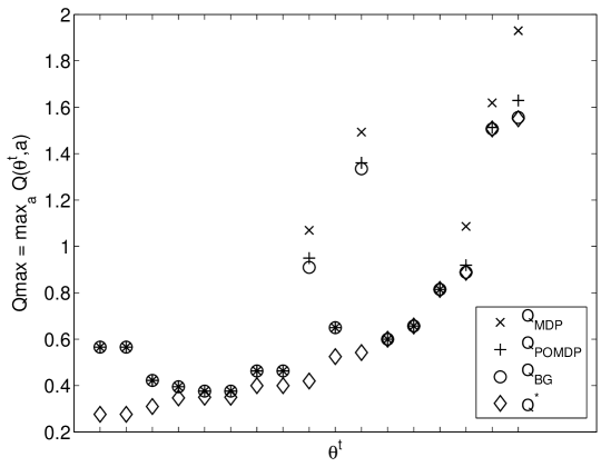
Figure 11: Comparison of maximal $Q(\vec{\theta}{}^{\,t},a)$-values for Meeting on a Grid. We plot the value of all $\theta^{t}$ that can be reached by an optimal policy, ordered according their optimal value.

Before providing a comparison of performance of some of the approximate Q-value functions described in this work, we will first give some more insights in their actual values. For the $h=4$ Dec-Tiger problem, we generated all possible $\vec{\theta}{}^{\,t}$ and the corresponding $P(\textrm{$s_{l}$}|\vec{\theta}{}^{\,t})$, according to (4.8). For each of these, the maximal $Q(\vec{\theta}{}^{\,t},a)$-value is plotted in Figure 10. Apart from the three approximate Q-value functions, we also plotted the optimal value for each joint action-observation history $\vec{\theta}{}^{\,t}$ that can be realized when using $\pi^{*}$. Note that different $\vec{\theta}{}^{\,t}$ can have different optimal values, but induce the same $P(\textrm{$s_{l}$}|\vec{\theta}{}^{\,t})$, as demonstrated in the figure: there are multiple $Q^{*}$-values plotted for some $P(\textrm{$s_{l}$}|\vec{\theta}{}^{\,t})$. For the horizon 3 Meeting on a Grid problem we also collected all $\vec{\theta}{}^{\,t}$ that can be visited by the optimal policy, and in Figure 11 we again plotted maximal $Q(\vec{\theta}{}^{\,t},a)$-values. Because this problem has many states, a representation as in Figure 10 is not possible. Instead, we ordered the $\vec{\theta}$ according to their optimal value. We can see that the bounds are tight for some $\vec{\theta}$, while for others they can be quite loose. However, when used in the ${\textrm{GMAA}^{*}}$ framework, their actual performance as a heuristic also depends on their valuation of $\vec{\theta}\in\vec{{\Theta}}$ not shown by Figure 11, namely those that will not be visited by an optimal policy: especially when these are overestimated, ${\textrm{GMAA}^{*}}$ will first examine a sub-optimal branch of the search tree. A tighter upper bound can speed up computation to a very large extent, as it allows the algorithm to prune the policy pool more, reducing the number of Bayesian games that need to be solved. Both figures clearly illustrate the main property of the upper bounds we discussed, namely that $Q^{*}\leq\textrm{Q}_{\textrm{BG}}\leq\textrm{Q}_{\textrm{POMDP}}\leq\textrm{Q}_{\textrm{MDP}}$ (see Theorem 5.1).

7.3 Computing Optimal Policies

As shown above, the hierarchy of upper bounds $Q^{*}\leq\textrm{Q}_{\textrm{BG}}\leq\textrm{Q}_{\textrm{POMDP}}\leq\textrm{Q}_{\textrm{MDP}}$ is not just a theoretical construct, but the differences in value specified can be significant for particular problems. In order to evaluate what the impact is of the differences between the approximate Q-value functions, we performed several experiments. Here we describe our evaluation of ${\textrm{MAA}^{*}}$ on a number of test problems using $\textrm{Q}_{\textrm{BG}}$, $\textrm{Q}_{\textrm{POMDP}}$ and $\textrm{Q}_{\textrm{MDP}}$ as heuristic. All timing results in this paper are CPU times with a resolution of $0.01$s, and were obtained on $3.4$GHz Intel Xeon processors.

$h$	$V^{*}$		$n_{\varphi}$	$T_{\textrm{GMAA}^{*}}$	$T_{Q}$
3	$5.1908$	$\textrm{Q}_{\textrm{MDP}}$	$105,228$	$0.31$ s	$0$ s
		$\textrm{Q}_{\textrm{POMDP}}$	$6,651$	$0.02$ s	$0$ s
		$\textrm{Q}_{\textrm{BG}}$	$6,651$	$0.02$ s	$0.02$ s
4	$4.8028$	$\textrm{Q}_{\textrm{MDP}}$	$37,536,938,118$	$431,776$ s	$0$ s
		$\textrm{Q}_{\textrm{POMDP}}$	$559,653,390$	$5,961$ s	$0.13$ s
		$\textrm{Q}_{\textrm{BG}}$	$301,333,698$	$3,208$ s	$0.94$ s

Table 1: ${\textrm{MAA}^{*}}$ results for Dec-Tiger.

$h$	$V^{*}$		$n_{\varphi}$	$T_{\textrm{GMAA}^{*}}$	$T_{Q}$
3	$5.8402$	$\textrm{Q}_{\textrm{MDP}}$	$151,236$	$0.46$ s	$0$ s
		$\textrm{Q}_{\textrm{POMDP}}$	$19,854$	$0.06$ s	$0.01$ s
		$\textrm{Q}_{\textrm{BG}}$	$13,212$	$0.04$ s	$0.03$ s
4	$11.1908$	$\textrm{Q}_{\textrm{MDP}}$	$33,921,256,149$	$388,894$ s	$0$ s
		$\textrm{Q}_{\textrm{POMDP}}$	$774,880,515$	$8,908$ s	$0.13$ s
		$\textrm{Q}_{\textrm{BG}}$	$86,106,735$	$919$ s	$0.92$ s

Table 2: ${\textrm{MAA}^{*}}$ results for Skewed Dec-Tiger.

Table 1 shows the results ${\textrm{MAA}^{*}}$ obtained on the original Dec-Tiger problem for horizon 3 and 4. It shows for each heuristic the number of partial joint policies evaluated $n_{\varphi}$, CPU time spent on the ${\textrm{GMAA}^{*}}$ phase $T_{{\textrm{GMAA}^{*}}}$, and CPU time spent on calculating the heuristic $T_{Q}$. As $\textrm{Q}_{\textrm{BG}}$, $\textrm{Q}_{\textrm{POMDP}}$ and $\textrm{Q}_{\textrm{MDP}}$ are upper bounds to $Q^{*}$, ${\textrm{MAA}^{*}}$ is guaranteed to find the optimal policy when using them as heuristic, however the timing results may differ.

For $h=3$ we see that using $\textrm{Q}_{\textrm{POMDP}}$ and $\textrm{Q}_{\textrm{BG}}$ only a fraction of the number of policies are evaluated when compared to $\textrm{Q}_{\textrm{MDP}}$ which reflects proportionally in the time spent on ${\textrm{GMAA}^{*}}$. For this horizon $\textrm{Q}_{\textrm{POMDP}}$ and $\textrm{Q}_{\textrm{BG}}$ perform the same, but the time needed to compute the $\textrm{Q}_{\textrm{BG}}$ heuristic is as long as the ${\textrm{GMAA}^{*}}$-phase, therefore $\textrm{Q}_{\textrm{POMDP}}$ outperforms $\textrm{Q}_{\textrm{BG}}$ here. For $h=4$, the impact of using tighter heuristics becomes even more pronounced. In this case the computation time of the heuristic is negligible, and $\textrm{Q}_{\textrm{BG}}$ outperforms both, as it is able to prune much more partial joint policies from the policy pool. Table 2 shows results for Skewed Dec-Tiger. For this problem the $\textrm{Q}_{\textrm{MDP}}$ and $\textrm{Q}_{\textrm{BG}}$ results are roughly the same as the original Dec-Tiger problem; for $h=3$ the timings are a bit slower, and for $h=4$ they are faster. For $\textrm{Q}_{\textrm{POMDP}},$ however, we see that for $h=4$ the results are slower as well and that $\textrm{Q}_{\textrm{BG}}$ outperforms $\textrm{Q}_{\textrm{POMDP}}$ by an order of magnitude.

$h$	$V^{*}$		$n_{\varphi}$	$T_{\textrm{GMAA}^{*}}$	$T_{Q}$
4	$3.8900$	$\textrm{Q}_{\textrm{MDP}}$	$328,212$	$3.54$ s	$0$ s
		$\textrm{Q}_{\textrm{POMDP}}$	$531$	$0$ s	$0.01$ s
		$\textrm{Q}_{\textrm{BG}}$	$531$	$0$ s	$0.03$ s
5	$4.7900$	$\textrm{Q}_{\textrm{MDP}}$	N/A	$>4.32\textrm{e}5$ s	$0$ s
		$\textrm{Q}_{\textrm{POMDP}}$	$196,883$	$5.30$ s	$0.20$ s
		$\textrm{Q}_{\textrm{BG}}$	$196,883$	$5.15$ s	$0.53$ s

Table 3: ${\textrm{MAA}^{*}}$ results for BroadcastChannel.

$h$	$V^{*}$		$n_{\varphi}$	$T_{\textrm{GMAA}^{*}}$	$T_{Q}$
2	$0.9100$	$\textrm{Q}_{\textrm{MDP}}$	$1,275$	$0$ s	$0$ s
		$\textrm{Q}_{\textrm{POMDP}}$	$1,275$	$0$ s	$0$ s
		$\textrm{Q}_{\textrm{BG}}$	$194$	$0$ s	$0$ s
3	$1.5504$	$\textrm{Q}_{\textrm{MDP}}$	$29,688,775$	$81.93$ s	$0$ s
		$\textrm{Q}_{\textrm{POMDP}}$	$3,907,525$	$10.80$ s	$0.15$ s
		$\textrm{Q}_{\textrm{BG}}$	$1,563,775$	$4.44$ s	$1.37$ s

Table 4: ${\textrm{MAA}^{*}}$ results for Meeting on a Grid.

$h$	$V^{*}$		$n_{\varphi}$	$T_{\textrm{GMAA}^{*}}$	$T_{Q}$
3	$-5.7370$	$\textrm{Q}_{\textrm{MDP}}$	$446,724$	$1.58$ s	$0.56$ s
		$\textrm{Q}_{\textrm{POMDP}}$	$26,577$	$0.08$ s	$0.21$ s
		$\textrm{Q}_{\textrm{BG}}$	$26,577$	$0.08$ s	$0.33$ s
4	$-6.5788$	$\textrm{Q}_{\textrm{MDP}}$	$25,656,607,368$	$309,235$ s	$0.85$ s
		$\textrm{Q}_{\textrm{POMDP}}$	$516,587,229$	$5,730$ s	$7.22$ s
		$\textrm{Q}_{\textrm{BG}}$	$516,587,229$	$5,499$ s	$11.72$ s

Table 5: ${\textrm{MAA}^{*}}$ results for Fire Fighting $\langle n_{h}=3,n_{f}=3\rangle$.

Results for the Broadcast Channel (Table 3), Meeting on a Grid (Table 4) and a Fire fighting problem (Table 5) are similar. The N/A entry in Table 3 indicates the $\textrm{Q}_{\textrm{MDP}}$ was not able to compute a solution within 5 days. For these problems we also see that the performance of $\textrm{Q}_{\textrm{POMDP}}$ and $\textrm{Q}_{\textrm{BG}}$ is roughly equal. For the Meeting on a Grid problem, $\textrm{Q}_{\textrm{BG}}$ yields a significant speedup over $\textrm{Q}_{\textrm{POMDP}}$.

7.4 Forward-Sweep Policy Computation

The ${\textrm{MAA}^{*}}$ results described above indicate that the use of a tighter heuristic can yield substantial time savings. In this section, the approximate Q-value functions are used in forward-sweep policy computation. We would expect that when using a Q-value function that more closely resembles $Q^{*}$, the quality of the resulting policy will be higher. We also tested whether ${k\textrm{-GMAA}^{*}}$ with $k>1$ improved the quality of the computed policies. In particular, we tested $k=1,2,\dots,5$.

$\vec{o}_{\emptyset}\to a_{\textrm{\tiny Li}}$

$o_{\textrm{\tiny HL}}\to a_{\textrm{\tiny Li}}$

$o_{\textrm{\tiny HR}}\to a_{\textrm{\tiny Li}}$

$o_{\textrm{\tiny HL}},o_{\textrm{\tiny HL}}\to a_{\textrm{\tiny OR}}$

$o_{\textrm{\tiny HL}},o_{\textrm{\tiny HR}}\to a_{\textrm{\tiny Li}}$

$o_{\textrm{\tiny HR}},o_{\textrm{\tiny HL}}\to a_{\textrm{\tiny Li}}$

$o_{\textrm{\tiny HR}},o_{\textrm{\tiny HR}}\to a_{\textrm{\tiny OL}}$

$o_{\textrm{\tiny HL}},o_{\textrm{\tiny HL}},o_{\textrm{\tiny HL}}\to a_{\textrm{\tiny Li}}$

$o_{\textrm{\tiny HL}},o_{\textrm{\tiny HL}},o_{\textrm{\tiny HR}}\to a_{\textrm{\tiny Li}}$

$o_{\textrm{\tiny HL}},o_{\textrm{\tiny HR}},o_{\textrm{\tiny HL}}\to a_{\textrm{\tiny Li}}$

$o_{\textrm{\tiny HL}},o_{\textrm{\tiny HR}},o_{\textrm{\tiny HR}}\to a_{\textrm{\tiny Li}}$

$o_{\textrm{\tiny HR}},o_{\textrm{\tiny HL}},o_{\textrm{\tiny HL}}\to a_{\textrm{\tiny Li}}$

$o_{\textrm{\tiny HR}},o_{\textrm{\tiny HL}},o_{\textrm{\tiny HR}}\to a_{\textrm{\tiny Li}}$

$o_{\textrm{\tiny HR}},o_{\textrm{\tiny HR}},o_{\textrm{\tiny HL}}\to a_{\textrm{\tiny Li}}$

$o_{\textrm{\tiny HR}},o_{\textrm{\tiny HR}},o_{\textrm{\tiny HR}}\to a_{\textrm{\tiny Li}}$

$\vec{o}_{\emptyset}\to a_{\textrm{\tiny Li}}$

$o_{\textrm{\tiny HL}}\to a_{\textrm{\tiny Li}}$

$o_{\textrm{\tiny HR}}\to a_{\textrm{\tiny Li}}$

$o_{\textrm{\tiny HL}},o_{\textrm{\tiny HL}}\to a_{\textrm{\tiny Li}}$

$o_{\textrm{\tiny HL}},o_{\textrm{\tiny HR}}\to a_{\textrm{\tiny Li}}$

$o_{\textrm{\tiny HR}},o_{\textrm{\tiny HL}}\to a_{\textrm{\tiny Li}}$

$o_{\textrm{\tiny HR}},o_{\textrm{\tiny HR}}\to a_{\textrm{\tiny Li}}$

$o_{\textrm{\tiny HL}},o_{\textrm{\tiny HL}},o_{\textrm{\tiny HL}}\to a_{\textrm{\tiny OR}}$

$o_{\textrm{\tiny HL}},o_{\textrm{\tiny HL}},o_{\textrm{\tiny HR}}\to a_{\textrm{\tiny Li}}$

$o_{\textrm{\tiny HL}},o_{\textrm{\tiny HR}},o_{\textrm{\tiny HL}}\to a_{\textrm{\tiny Li}}$

$o_{\textrm{\tiny HL}},o_{\textrm{\tiny HR}},o_{\textrm{\tiny HR}}\to a_{\textrm{\tiny Li}}$

$o_{\textrm{\tiny HR}},o_{\textrm{\tiny HL}},o_{\textrm{\tiny HL}}\to a_{\textrm{\tiny Li}}$

$o_{\textrm{\tiny HR}},o_{\textrm{\tiny HL}},o_{\textrm{\tiny HR}}\to a_{\textrm{\tiny Li}}$

$o_{\textrm{\tiny HR}},o_{\textrm{\tiny HR}},o_{\textrm{\tiny HL}}\to a_{\textrm{\tiny Li}}$

$o_{\textrm{\tiny HR}},o_{\textrm{\tiny HR}},o_{\textrm{\tiny HR}}\to a_{\textrm{\tiny OL}}$

Figure 12: Policies found using forward-sweep policy computation (i.e., $k=1$) for the $h=4$ Dec-Tiger problem. Left: the policy resulting from $\textrm{Q}_{\textrm{MDP}}$. Right: the optimal policy as calculated by $\textrm{Q}_{\textrm{POMDP}}$ and $\textrm{Q}_{\textrm{BG}}$. The framed entries highlight the crucial differences.

\psfrag{V}{\scriptsize$V$}\psfrag{k}{\scriptsize$k$}\includegraphics[height=85.35826pt]{results/dectiger_skewed/OFS_dectiger_skewed_h3}

(a) Skewed Dec-Tiger, $h=3$.

\psfrag{V}{\scriptsize$V$}\psfrag{k}{\scriptsize$k$}\includegraphics[height=85.35826pt]{results/dectiger_skewed/OFS_dectiger_skewed_h4}

(b) Skewed Dec-Tiger, $h=4$.

\psfrag{V}{\scriptsize$V$}\psfrag{k}{\scriptsize$k$}\includegraphics[height=85.35826pt]{results/GridSmall/OFS_GridSmall_h3}

(c) GridSmall, $h=3$.

\psfrag{V}{\scriptsize$V$}\psfrag{k}{\scriptsize$k$}\includegraphics[height=85.35826pt]{results/fireFighting_2_3_3/OFS_fireFighting_2_3_3_h4}

(d) FireFighting with $\langle n_{h}=3,n_{f}=3\rangle$, $h=4$.

\psfrag{V}{\scriptsize$V$}\psfrag{k}{\scriptsize$k$}\includegraphics[height=85.35826pt]{results/fireFighting_2_4_3/OFS_fireFighting_2_4_3_h3}

(e) FireFighting with $\langle n_{h}=4,n_{f}=3\rangle$, $h=3$.

\psfrag{V}{\scriptsize$V$}\psfrag{k}{\scriptsize$k$}\includegraphics[height=85.35826pt]{results/fireFighting_2_4_3/OFS_fireFighting_2_4_3_h4}

(f) FireFighting with $\langle n_{h}=4,n_{f}=3\rangle$, $h=4$.

Figure 13: ${k\textrm{-GMAA}^{*}}$ results for different problems and horizons. The $y$-axis indicates value of the initial joint belief, while the $x$-axis denotes $k$.

For the Dec-Tiger problem, ${k\textrm{-GMAA}^{*}}$ with $k=1$ (and thus also $2\leq k\leq 5$) found the optimal policy (with $V(\pi^{*})=5.19$) for horizon $3$ using all approximate Q-value functions. For horizon $h=4$, also all different values of $k$ produced the same result for each approximate Q-value function. In this case, however, $\textrm{Q}_{\textrm{MDP}}$ found a policy with expected return of $3.19$. $\textrm{Q}_{\textrm{POMDP}}$ and $\textrm{Q}_{\textrm{BG}}$ did find the optimal policy ($V(\pi^{*})=4.80)$. Figure 12 illustrates the optimal policy (right) and the one found by $\textrm{Q}_{\textrm{MDP}}$ (left). It shows that $\textrm{Q}_{\textrm{MDP}}$ overestimates the value for opening the door in stage $t=2$.

For the Skewed Dec-Tiger problem, different values of $k$ did produce different results. In particular, for $h=3$ only $\textrm{Q}_{\textrm{BG}}$ finds the optimal policy (and thus attains the optimal value) for all values of $k$, as shown in Figure 13(a). $\textrm{Q}_{\textrm{POMDP}}$ does find it starting from $k=2$, and $\textrm{Q}_{\textrm{MDP}}$ only from $k=5$. Figure 13(b) shows a somewhat unexpected result for $h=4$: here for $k=1$ $\textrm{Q}_{\textrm{MDP}}$ and $\textrm{Q}_{\textrm{BG}}$ find the optimal policy, but $\textrm{Q}_{\textrm{POMDP}}$ doesn’t. This clearly illustrates that a tighter approximate Q-value function is not a guarantee for a better joint policy, which is also illustrated by the results for GridSmall in Figure 13(c).

We also performed the same experiment for two settings of the FireFighting problem. For $\langle n_{h}=3,n_{f}=3\rangle$ and $h=3$ all Q-value functions found the optimal policy (with value $-5.7370$) for all $k$, and horizon $4$ is shown in Figure 13(d). Figures 13(e) and 13(f) show the results for $\langle n_{h}=4,n_{f}=3\rangle$. For $h=4$, $\textrm{Q}_{\textrm{MDP}}$ did not finish for $k\geq 3$ within 5 days.

It is encouraging that for all experiments ${k\textrm{-GMAA}^{*}}$ using $\textrm{Q}_{\textrm{BG}}$ and $\textrm{Q}_{\textrm{POMDP}}$ with $k\leq 2$ found the optimal policy. Using $\textrm{Q}_{\textrm{MDP}}$ the optimal policy was also always found with $k\leq 5$, except in horizon $4$ Dec-Tiger and the $\langle n_{h}=4,n_{f}=3\rangle$ FireFighting problem. These results seem to indicate that this type of approximation might be likely to produce (near-) optimal results for other domains as well.

8 Conclusions

A large body of work in single-agent decision-theoretic planning is based on value functions, but such theory has been lacking thus far for Dec-POMDPs. Given the large impact of value functions on single-agent planning under uncertainty, we expect that a thorough study of value functions for Dec-POMDPs can greatly benefit multiagent planning under certainty. In this work, we presented a framework of Q-value functions for Dec-POMDPs, providing a significant contribution to fill this gap in Dec-POMDP theory. Our theoretical contributions have lead to new insights, which we applied to improve and extend solution methods.

We have shown how an optimal joint policy $\pi^{*}$ induces an optimal Q-value function $Q^{*}(\vec{\theta}{}^{\,t},a)$, and how it is possible to construct the optimal policy $\pi^{*}$ using forward-sweep policy computation. This entails solving Bayesian games for time steps $t=0\,,...,\,h-1$ which use $Q^{*}(\vec{\theta}{}^{\,t},a)$ as the payoff function. Because there is no clear way to compute $Q^{*}(\vec{\theta}{}^{\,t},a)$, we introduced a different description of the optimal Q-value function $Q^{*}(\vec{\theta}{}^{\,t},\varphi^{t+1})$ that is based on sequential rationality. This new description of $Q^{*}$ can be computed using dynamic programming and can then be used to construct $\pi^{*}$.

Because calculating $Q^{*}$ is computationally expensive, we examined approximate Q-value functions that can be calculated more efficiently and we discussed how they relate to $Q^{*}$. We covered $\textrm{Q}_{\textrm{MDP}}$, $\textrm{Q}_{\textrm{POMDP}}$, and $\textrm{Q}_{\textrm{BG}}$, a recently proposed approximate Q-value function. Also, we established that decreasing communication delays in decentralized systems cannot decrease the expected value and thus that $Q^{*}\leq\textrm{Q}_{\textrm{BG}}\leq\textrm{Q}_{\textrm{POMDP}}\leq\textrm{Q}_{\textrm{MDP}}$. Experimental evaluation indicated that these upper bounds are not just of theoretical interest, but that significant differences exist in the tightness of the various approximate Q-value functions.

Additionally we showed how the approximate Q-value functions can be used as heuristics in a generalized policy search method ${\textrm{GMAA}^{*}}$, thereby unifying forward-sweep policy computation and the recent Dec-POMDP solution techniques of ? (?) and ? (?). Finally, we performed an empirical evaluation of ${\textrm{GMAA}^{*}}$ showing significant reductions in computation time when using tighter heuristics to calculate optimal policies. Also $\textrm{Q}_{\textrm{BG}}$ generally found better approximate solutions in forward-sweep policy computation and the ‘$k$-best joint BG policies’ ${\textrm{GMAA}^{*}}$ variant, or ${k\textrm{-GMAA}^{*}}$.

There are quite a few directions for future research. One is to try to extend the results of this paper to partially observable stochastic games (POSGs) (?), which are Dec-POMDPs with an individual reward function for each agent. Since the dynamics of the POSG model are identical to those of a Dec-POMDP, a similar modeling via Bayesian games is possible. An interesting question is whether also in this case, an optimal (i.e., rational) joint policy can be found by forward-sweep policy computation.

Staying within the context of Dec-POMDPs, a research direction could be to further generalize ${\textrm{GMAA}^{*}}$, by defining other Next or Select operators, with the hope that the resulting algorithms will be able to scale to larger problems. Also it is important to establish bounds on the performance and learning curves of ${\textrm{GMAA}^{*}}$ in combination with different Next operators and heuristics. A different direction is to experimentally evaluate the use of even tighter heuristics such as Q-value functions for the case of observations delayed by multiple time steps. This research should be paired with methods to efficiently find such Q-value functions. Finally, future research should further examine Bayesian games. In particular, the work of ? (?) could be used as a starting point for further research to approximately modeling Dec-POMDPs using BGs. Finally, there is a need for efficient approximate methods for solving the Bayesian games.

A Proofs

A.1 There is At Least One Optimal Pure Joint Policy

Proposition (2.1).

A Dec-POMDP has at least one optimal pure joint policy.

Proof.

This proof follows a proof by ? (?). It is possible to convert a Dec-POMDP to an extensive game and thus to a strategic game, in which the actions are pure policies for the Dec-POMDP (?). In this strategic game, there is at least one maximizing entry corresponding to a pure joint policy which we denote $\pi_{\textrm{max}}$. Now, assume that there is a joint stochastic policy $\varsigma=\left\langle\varsigma_{1},\dots,\varsigma_{n}\right\rangle$ that attains a higher payoff. ? (?) showed that for each stochastic $\varsigma_{i}$ policy, there is a corresponding mixed policy $\mu_{i}$. Therefore $\varsigma$ corresponds to a joint mixed policy $\mu=\left\langle\mu_{1},\dots,\mu_{n}\right\rangle$. Let us write $\Pi_{i,\mu_{i}}$ for the support of $\mu_{i}$. $\mu$ now induces a probability distribution $P_{\mu}$ over the set of joint policies $\Pi_{\mu}=\Pi_{1,\mu_{1}}\times\dots\times\Pi_{n,\mu_{n}}\subseteq\Pi$ which is a subset of the set of all joint policies. The expected payoff can now be written as

$$V(\varsigma)=E_{P_{\mu}}(V(\pi)|\pi\in\Pi_{\mu})\leq\max_{\pi\in\Pi}V(\pi)=V(\pi_{\textrm{max}}),$$

contradicting that $\varsigma$ is a joint stochastic policy that attains a higher payoff.∎

A.2 Hierarchy of Q-value Functions

This section lists the proof of theorem 5.1. It is ordered as follows. First, Section A.2.1 presents a model and resulting value functions for Dec-POMDPs with $k$-steps delayed communication. Next, Section A.2.2 shows that $\textrm{Q}_{\textrm{POMDP}},$ $\textrm{Q}_{\textrm{BG}}$ and $Q^{*}$ correspond with the case that $k$ is respectively $0$, 1 and $h$. Finally, Section A.2.3 shows that when the communication delay $k$ increases, the optimal expected return cannot decrease, thereby proving theorem 5.1.

A.2.1 Modeling Dec-POMDPs with $k$-Steps Delayed Communication

\psfrag{a11}[cc][b]{\small$a_{1}$}\psfrag{a12}[cc][b]{\small$\bar{a}_{1}$}\psfrag{a21}[cc][b]{\small$a_{2}$}\psfrag{a22}[cc][b]{\small$\bar{a}_{2}$}\psfrag{o11}[cc][b]{\small$o_{1}$}\psfrag{o12}[cc][b]{\small$\bar{o}_{1}$}\psfrag{o21}[cc][b]{\small$o_{2}$}\psfrag{o22}[cc][b]{\small$\bar{o}_{2}$}\psfrag{pol1}[cc][c]{\small{ $q_{1}^{t}$ } }\psfrag{pol2}[cc][c]{\small{ $q_{2}^{t}$ } }\psfrag{polBG}[cc][c]{\small$\beta^{t+k}$}\psfrag{o12o21}[lc][b]{\small$o^{t+1}=\langle\bar{o}_{1},o_{2}\rangle$}\psfrag{pol1b}[cc][lc]{\small{ $q_{1}^{t+1}$ } }\psfrag{pol2b}[cc][lc]{\small{ $q_{2}^{t+1}$ } }\psfrag{t-k}[cc][c]{\small$t$}\psfrag{t-k+1}[cc][c]{\small$t+1$}\psfrag{t-1}[cc][c]{\small$t+k-1$}\psfrag{t}[cc][c]{\small$t+k$}\includegraphics[width=346.89731pt]{figs/joint_pol_expanding+shifting}

Figure 14: Policies specified by the states of the augmented MDP for $k=2$. Top: policies for $\hat{s}^{t}$. The policy extended by augmented MDP action $\hat{a}^{t}=\beta$ is shown dashed. Bottom: The resulting policies after for joint observation $\left\langle\bar{o}_{1},o_{2}\right\rangle$.

Here we present an augmented MDP that can be used to find the optimal solution for Dec-POMDPs with $k$ steps delayed communication. This is a reformulation of the work by ? (?) and ? (?), extended to the Dec-POMDP setting. We define this augmented MDP as $\hat{M}=\langle\hat{\mathcal{S}},\hat{\mathcal{A}},\hat{T},\hat{R}\rangle$, where the augmented MDP stages are indicated $\hat{t}$.

The state space is $\hat{\mathcal{S}}=(\hat{\mathcal{S}}^{\hat{t}=0},\dots,\hat{\mathcal{S}}^{\hat{t}=h-1})$. An augmented state is composed of a joint action-observation history, and a joint policy tree $q^{t}$.

$$\hat{s}^{\hat{t}=t}=\begin{cases}\langle\vec{\theta}{}^{\,t},q^{t}\rangle&,\,0\leq t\leq h-k-1\\ \langle\vec{\theta}{}^{\,t},q^{\tau=h-t,t}\rangle&,\,h-k\leq t\leq h-1\end{cases}.$$

The contained $q^{t}$ is a joint depth-$k$ (specifying actions for $k$ stages) joint policy tree $q^{t}=\left\langle q_{1}^{t},...,q_{n}^{t}\right\rangle$, to be used starting at stage $t$. For the last $k$ stages, the contained joint policy $q^{\tau=h-t,t}$ specifies $\tau=h-t\leq k$ stages.

$\hat{\mathcal{A}}$ is the set of augmented actions. For $0\leq\hat{t}\leq h-k-1$, an action $\hat{a}^{\hat{t}}\in\hat{\mathcal{A}}$ is a joint policy $\hat{a}^{\hat{t}=t}=\beta^{t+k}=\langle\beta_{1}^{t+k}\dots\beta_{n}^{t+k}\rangle$ implicitly mapping length-$k$ observation histories to joint actions to be taken at stage $t+k$. I.e., $\beta_{i}^{t+k}:\vec{\mathcal{O}}_{i}^{k}\rightarrow\mathcal{A}_{i}^{{t+k}}$. For the last $k$ stages $h-k\leq\hat{t}\leq h-1$ there only is one empty action $a_{\emptyset}$ that has no influence whatsoever.

The augmented actions are used to expand the joint policy trees. When ‘appending’ a policy $\beta^{t+k}$ to $q^{t}$ we form a depth $k+1$ policy, which we denote $q^{\tau=k+1,t}=\langle{q^{t}}\circ{\beta^{t+k}}\rangle$. After execution of its initial joint action $q^{\tau=k+1,t}(\vec{o}_{\emptyset})$ and receiving a particular joint observation $o$, a $q^{\tau=k+1,t}$ reduces to its depth $k$ sub-tree policy for that particular joint observation, denoted $q^{t-k+1}=q^{\tau=k+1,t}(o)=\langle{q^{t-k}}\circ{\beta^{t}}\rangle(o)$. This is illustrated in Figure 14.

\psfrag{a11}[cc][b]{\small$a_{1}$}\psfrag{a12}[cc][b]{\small$\bar{a}_{1}$}\psfrag{a21}[cc][b]{\small$a_{2}$}\psfrag{a22}[cc][b]{\small$\bar{a}_{2}$}\psfrag{o11}[cc][b]{\small$o_{1}$}\psfrag{o12}[cc][b]{\small$\bar{o}_{1}$}\psfrag{o21}[cc][b]{\small$o_{2}$}\psfrag{o22}[cc][b]{\small$\bar{o}_{2}$}\psfrag{hata}[bl][bl]{\small{$o^{t+1}=\langle o_{1},o_{2}\rangle$} }\psfrag{s^t-k}[cl][bl]{\small$\vec{\theta}{}^{\,t},$}\psfrag{s^t+1-k}[cl][bl]{\small$\vec{\theta}{}^{\,t+1},$}\psfrag{hst}[cc][c]{\small$\hat{s}^{t}$}\psfrag{hst+}[cc][c]{\small$\hat{s}^{t+1}$}\psfrag{t-k}[cc][b]{\small$t$}\psfrag{t-1}[cc][b]{\small$t+1$}\psfrag{(t+1)-k}[cc][b]{\small$t+1$}\psfrag{(t+1)-1}[cc][b]{\small$t+k$}\includegraphics[scale={0.72}]{figs/Ooi_MDP_illustr}

Figure 15: An illustration of the augmented MDP with $k=2$, showing a transition from $\hat{s}^{t}$ to $\hat{s}^{t+1}$ by action $\hat{a}=\beta^{t}$. In this example $\vec{\theta}{}^{\,t-k+1}=(\vec{\theta}{}^{\,t-k+1},\left\langle a_{1},a_{2}\right\rangle,\left\langle\bar{o}_{1},o_{2}\right\rangle)$. The actions specified for stage $t$ are given by $\beta^{t}(\left\langle\bar{o}_{1},o_{2}\right\rangle)$ as depicted in Figure 14.

$\hat{T}$ is the transition model. A probability $P(\hat{s}^{\hat{t}+1}|\hat{s}^{\hat{t}},\hat{a}^{\hat{t}})$ for stage $\hat{t}=t$ translates as follows for $0\leq t\leq h-k-1$

$$P(\langle\vec{\theta}{}^{\,t+1},q^{t+1}\rangle|\langle\vec{\theta}{}^{\,t},q^{t}\rangle,\beta^{t+k})=\begin{cases}P(o^{t+1}|\vec{\theta}{}^{\,t},q^{t}(\vec{o}_{\emptyset}))&\textrm{if conditions hold,}\\ 0&\textrm{otherwise,}\end{cases}$$ (A.1)

where the conditions are: 1) $q^{t+1}=\langle{q^{t}}\circ{\beta^{t+k}}\rangle(o^{t+1})$, and 2) $\vec{\theta}{}^{\,t+1}=(\vec{\theta}{}^{\,t},a^{t},o^{t+1})$. For $h-k\leq t\leq h-1$, $\beta^{t+k}$ in (A.1) reduces to $a_{\emptyset}$. The probabilities are unaffected, but the first condition changes to $q^{\tau=h-t-1,t+1}=q^{\tau=h-t,t}(o^{t+1})$.

Finally, $\hat{R}$ is the reward model, which is specified as follows:

$$\forall_{0\leq t\leq h-1}\quad\hat{R}(\hat{s}^{\hat{t}=t})=\hat{R}(\langle\vec{\theta}{}^{\,t},q^{t}\rangle)=R(\vec{\theta}{}^{\,t},q^{t}(\vec{o}_{\emptyset})),$$ (A.2)

where $q^{t}(\vec{o}_{\emptyset})$ is the initial joint action specified by $q^{t}$. $R(\vec{\theta}{}^{\,t},a)$ is defined as before in (2.12).

The resulting optimality equations $\hat{Q}^{\hat{t}}(\hat{s},\hat{a})$ for the augmented MDP are as follows. We will write $Q_{k}$ for the optimal Q-value function for a $k$-steps delayed communication system. We will also refer to this as the $k\textrm{-Q}_{\textrm{BG}}$ value function.

$$\forall_{0\leq t\leq h-k-1}\quad Q_{k}(\vec{\theta}{}^{\,t},q^{t},\beta^{t+k})=R(\vec{\theta}{}^{\,t},q^{t}(\vec{o}_{\emptyset}))+\sum_{o^{t+1}\in\mathcal{O}}P(o^{t+1}|\vec{\theta}{}^{\,t},q^{t}(\vec{o}_{\emptyset}))Q_{k}^{*}(\vec{\theta}{}^{\,t+1},q^{t+1}),$$ (A.3)

with $q^{t+1}=\langle{q^{t}}\circ{\beta^{t+k}}\rangle(o^{t+1})$ and where

$$Q_{k}^{*}(\vec{\theta}{}^{\,t},q^{t})\ \operatorname{\equiv}\ \max_{\beta^{t+k}}Q_{k}(\vec{\theta}{}^{\,t},q^{t},\beta^{t+k}).$$ (A.4)

For the last $k$ stages, $h-k\leq t\leq h-1$, there are $\tau^{\prime}=h-t$ stages to go and we get

$$Q_{k}^{*}(\vec{\theta}{}^{\,t},q^{\tau=\tau^{\prime},t})=R(\vec{\theta}{}^{\,t},q^{\tau=\tau^{\prime},t}(\vec{o}_{\emptyset}))+\sum_{o^{t+1}}P(o^{t+1}|\vec{\theta}{}^{\,t},q^{\tau=\tau^{\prime},t}(\vec{o}_{\emptyset}))Q_{k}^{*}(\vec{\theta}{}^{\,t+1},q^{\tau=\tau^{\prime}-1,t+1}).$$ (A.5)

Note that (A.5) does not include any augmented actions $\hat{a}^{\hat{t}=t}=\beta^{t+k}$. Therefore, the last $k$ stages should be interpreted as a Markov chain. Standard dynamic programming can be applied to calculate all $Q^{*}(\vec{\theta}{}^{\,t},q^{t})$-values.

A.2.2 Relation of $k\textrm{-Q}_{\textrm{BG}}$ with Other Approximate Q-value Functions

Here we briefly show how $k\textrm{-Q}_{\textrm{BG}}$ in fact reduces to some of the cases treated earlier.

For $k=0$, $k\textrm{-Q}_{\textrm{BG}}$ (A.3) reduces to $\textrm{Q}_{\textrm{POMDP}}$. In the $k=0$ case, $q^{t-k}$ becomes a depth-0, i.e. empty, policy. Also, $\beta^{t}$ becomes a mapping from length-0 observation histories to actions, i.e., it becomes a joint action. Substitution in (A.3) yields

$$Q_{0}(\left\langle\vec{\theta}{}^{\,t},\emptyset\right\rangle,a^{t})=R(\vec{\theta}{}^{\,t},a^{t})+\sum_{o^{t+1}}P(o^{t+1}|\vec{\theta}{}^{\,t},a^{t})\max_{a^{t+1}}Q_{0}(\left\langle\vec{\theta}{}^{\,t+1},\emptyset\right\rangle,a^{t+1}).$$

Now, as ${\widehat{Q}}_{\textrm{P}}(\vec{\theta}{}^{\,t},a)\ \operatorname{\equiv}\ {Q}_{\textrm{P}}^{*}(b^{\vec{\theta}{}^{\,t}},a),$ this clearly corresponds to the $\textrm{Q}_{\textrm{POMDP}}$-value function (5.6).

${1}\textrm{-Q}_{\textrm{BG}}$ reduces to regular $\textrm{Q}_{\textrm{BG}}$. Notice that for $k=1,$ $q^{\tau=k,t}$ reduces to $a^{t}$. Filling out yields:

$$Q_{1}(\left\langle\vec{\theta}{}^{\,t},a^{t}\right\rangle,\beta^{t+1})=R(\vec{\theta}{}^{\,t},a^{t})+\sum_{o^{t+1}}P(o^{t+1}|\vec{\theta}{}^{\,t},a^{t})\max_{\beta^{t+2}}Q_{1}(\left\langle\vec{\theta}{}^{\,t+1},\beta^{t+1}(o^{t+1})\right\rangle,\beta^{t+2}).$$

Now using (A.4) we obtain the $\textrm{Q}_{\textrm{BG}}$-value function (5.12).

A Dec-POMDP is identical to an $h$-steps delayed communication system. Augmented states have the form $\hat{s}^{\hat{t}=0}=\langle\vec{\theta}_{\emptyset},q^{0}\rangle$, where $q^{0}=\pi$ specifies a full length $h$ joint policy. The first stage $t=0$ in this augmented MDP, is also one of the last $k$ $(=h)$ stages. Therefore, the applied $Q$-function is (A.5), which means that the Markov chain evaluation starts immediately. Effectively this boils down to evaluation of all joint policies (corresponding to all augmented start states). The maximizing one specifies the value function of an optimal joint policy $Q^{*}.$

A.2.3 Shorter Communication Delays cannot Decrease the Value

First, we introduce some notation. Let us write $P_{o}$ for all the observation probabilities given $\vec{\theta}{}^{\,t},q^{t}$ and the sequence of ‘intermediate observations’ $(o^{t+1},\dots,o^{t+l-1})$

$$P_{o}(o^{t+l})\ \operatorname{\equiv}\ P\left[o^{t+l}|(\vec{\theta}{}^{\,t},q^{t}(\vec{o}_{\emptyset}),o^{t+1},q^{t}(o^{t+1}),\dots,o^{t+l-1}),q^{t}(o^{t+l-1})\right],\qquad\forall l\leq k.$$ (A.6)

In order to avoid confusion, we write $\beta^{t}_{|k|}$ for a policy that implicitly maps $k$-length observation histories to actions, and $\beta^{t}_{|k+1|}$ for one that is a mapping from length $(k+1)$ observation-histories to actions.

Now we give a reformulation of $Q_{k}$. $Q_{k}^{t,*}(\vec{\theta}{}^{\,t},q^{t})$ specifies the expected return for $\vec{\theta}{}^{\,t},q^{t}$ over stages $t,t+1,\dots,h-1$. Here, we will split this

$$Q_{k}^{*}(\vec{\theta}{}^{\,t},q^{t})=K_{k}(\vec{\theta}{}^{\,t},q^{t})+F_{k}^{t,*}(\vec{\theta}{}^{\,t},q^{t})$$ (A.7)

in $K_{k}(\vec{\theta}{}^{\,t},q^{t})$, the expected $k$-step reward, i.e., the expected return over for stages $t,\dots,t+k-1$ and $F_{k}^{t,*}(\vec{\theta}{}^{\,t},q^{t})$, the expected return over stages $t+k,t+k+1,\dots,h-1$, referred to as the ‘in $k$-steps’ expected return.

The former is defined as

$$K_{k}(\vec{\theta}{}^{\,t},q^{t})\ \operatorname{\equiv}\ E\left[\sum_{t^{\prime}=t}^{t+k-1}R(\vec{\theta}{}^{\,t^{\prime}},a^{t^{\prime}})\,\Big{|}\,\vec{\theta}{}^{\,t},q^{t}\right].$$ (A.8)

Let us define $K^{\tau=i}(\vec{\theta}{}^{\,t},q^{\tau=i,t})$ as the expected reward for the next $i$ stages, i.e.,

$$K_{k}(\vec{\theta}{}^{\,t},q^{t})=K^{\tau=k}(\vec{\theta}{}^{\,t},q^{t}).$$ (A.9)

We then have $K^{\tau=1}(\vec{\theta}{}^{\,t},a^{t})=R(\vec{\theta}{}^{\,t},a^{t})$ and

$$K^{\tau=i}(\vec{\theta}{}^{\,t},q^{\tau=i,t})=R(\vec{\theta}{}^{\,t},q^{\tau=i,t}(\vec{o}_{\emptyset}))+\\ \sum_{o^{t+1}}P(o^{t+1}|\vec{\theta}{}^{\,t},q^{\tau=i,t}(\vec{o}_{\emptyset}))K^{\tau=i-1}(\vec{\theta}{}^{\,t+1},q^{\tau=i-1,t+1}(o^{t+1})),$$ (A.10)

where $q^{\tau=i-1,t+1}(o^{t+1})$ is the depth-$(i-1)$ joint policy that results from $q^{\tau=i,t}$ after observation of $o^{t+1}$.

If we define $F_{k}^{\tau=i,t}(\vec{\theta}{}^{\,t},q^{t},\beta^{t+k}_{|k|})$ to be the expected reward for stages $t+i,t+i+1,\dots,h-1$. That is, the time-to-go $\tau=i$ denotes how much time-to-go before we start accumulating expected reward. The ‘in $k$-steps’ expected return is then given by

$$F_{k}^{t}(\vec{\theta}{}^{\,t},q^{t},\beta^{t+k}_{|k|})=F_{k}^{\tau=k,t}(\vec{\theta}{}^{\,t},q^{t},\beta^{t+k}_{|k|}).$$

The evaluation is then performed by

$$F_{k}^{\tau=0,t}(\vec{\theta}{}^{\,t},q^{t},\beta^{t+k}_{|k|}) = Q_{k}(\vec{\theta}{}^{\,t},q^{t},\beta^{t+k}_{|k|})$$ (A.11)

$$F_{k}^{\tau=i,t}(\vec{\theta}{}^{\,t},q^{t},\beta^{t+k}_{|k|}) = \sum_{o^{t+1}}P_{o}(o^{t+1})F_{k}^{\tau=i-1,t+1,*}(\vec{\theta}{}^{\,t+1},q^{t+1}),$$ (A.12)

where $q^{t+1}=\langle{q^{t+1}}\circ{\beta^{t+k}_{|k|}}\rangle(o^{t+1})$, and where

$$F_{k}^{\tau=i,t,*}(\vec{\theta}{}^{\,t},q^{t})=\max_{\beta^{t+k}_{|k|}}F_{k}^{\tau=i,t}(\vec{\theta}{}^{\,t},q^{t},\beta^{t+k}_{|k|}).$$ (A.13)

Theorem A.1 (Shorter communication delays cannot decrease the value).

The optimal Q-value function $Q_{k}$ of a finite horizon Dec-POMDP with $k$-steps delayed communication is an upper bound to $Q_{k+1}$, that of a $k+1$-steps delayed communication system. That is

$$\forall_{t}\forall_{\vec{\theta}{}^{\,t}}\forall_{q^{\tau=k,t},\beta^{t+k}_{|k|}}\quad Q_{k}(\vec{\theta}{}^{\,t},q^{\tau=k,t},\beta^{t+k}_{|k|})\geq\max_{\beta^{t+k+1}_{|k+1|}}Q_{k+1}(\vec{\theta}{}^{\,t},\langle{q^{\tau=k,t}}\circ{\beta^{t+k}_{|k|}}\rangle,\beta^{t+k+1}_{|k+1|}).$$ (A.14)

Proof.

The proof is by induction. The base case is that (A.14) holds for stages $h-(k+1)\leq t\leq h-1$, as shown by lemma A.1. The induction hypothesis states that, assuming (A.14) holds for some stage $t+k$, it also holds for stage $t$. The induction step is proven in lemma A.2. ∎

Lemma A.1 (Base case).

For all $h-k-1\leq t\leq h-1$, the expected cumulative future reward under $k$ steps delay is equal to that under $k+1$ steps delay if the same policies are followed from that point. That is,

$$\forall_{h-k\leq t\leq h-1}\forall_{\vec{\theta}{}^{\,t}}\forall_{q^{\tau=h-t,t}}\quad Q_{k}^{*}(\vec{\theta}{}^{\,t},q^{\tau=h-t,t})=Q_{k+1}^{*}(\vec{\theta}{}^{\,t},q^{\tau=h-t,t}),$$ (A.15)

and $\forall_{\vec{\theta}{}^{\,h-k-1}}\forall_{q^{\tau=k,h-k-1},\beta^{h-1}_{|k|}}$

$$Q_{k}(\vec{\theta}{}^{\,h-k-1},q^{\tau=k,h-k-1},\beta^{h-1}_{|k|})=Q_{k+1}(\vec{\theta}{}^{\,h-k-1},\langle{q^{\tau=k,h-k-1}}\circ{\beta^{h-1}_{|k|}}\rangle).$$ (A.16)

Proof.

For a particular stage $t=h-\tau^{\prime}$ with $h-k\leq t\leq h-1$ and an arbitrary $\vec{\theta}{}^{\,t},q^{\tau=\tau^{\prime},t}$, we can write

$$Q_{k}^{*}(\vec{\theta}{}^{\,t},q^{\tau=\tau^{\prime},t})=Q_{k+1}^{*}(\vec{\theta}{}^{\,t},q^{\tau=\tau^{\prime},t}),$$

because both are given by the evaluation of (A.5), and this evaluation involves no actions: Basically (A.5) has reduced to a Markov chain, and this Markov chain is the same for $Q_{k}^{*}$ and $Q_{k+1}^{*}$. We can conclude that

$$\forall_{h-k\leq t\leq h-1}\forall_{\vec{\theta}{}^{\,t},q^{\tau=\tau^{\prime},t}}\quad Q_{k}^{*}(\vec{\theta}{}^{\,t},q^{\tau=\tau^{\prime},t})=Q_{k+1}^{*}(\vec{\theta}{}^{\,t},q^{\tau=\tau^{\prime},t}).$$

Now we will prove (A.16). The left side of (A.16) is given by application of (A.3)

$$Q_{k}(\vec{\theta}{}^{\,h-k-1},q^{\tau=k,h-k-1},\beta^{h-1}_{|k|})=R(\vec{\theta}{}^{\,h-k-1},q^{\tau=k,h-k-1}(\vec{o}_{\emptyset}))+\\ \sum_{o^{h-k}}P(o^{h-k}|\vec{\theta}{}^{\,h-k-1},q^{\tau=k,h-k-1}(\vec{o}_{\emptyset}))Q_{k}^{*}(\vec{\theta}{}^{\,h-k},q^{\tau=k,h-k}),$$

with $q^{\tau=k,h-k}=\langle{q^{\tau=k,h-k-1}}\circ{\beta^{h-1}_{|k|}}\rangle(o^{h-k})$. The right side is given by application of (A.5)

$$Q_{k+1}(\vec{\theta}{}^{\,h-k-1},\langle{q^{\tau=k,h-k-1}}\circ{\beta^{h-1}_{|k|}}\rangle)=R(\vec{\theta}{}^{\,h-k-1},q^{\tau=k,h-k-1}(\vec{o}_{\emptyset}))+\\ \sum_{o^{h-k}}P(o^{h-k}|\vec{\theta}{}^{\,h-k-1},q^{\tau=k,h-k-1}(\vec{o}_{\emptyset}))Q_{k+1}^{*}(\vec{\theta}{}^{\,h-k},q^{\tau=k,h-k})$$

with $q^{\tau=k,h-k}=\langle{q^{\tau=k,h-k-1}}\circ{\beta^{h-1}_{|k|}}\rangle(o^{h-k})$. Now, because the policies $q^{\tau=k,h-k}$ are the same, we get

$$Q_{k}^{*}(\vec{\theta}{}^{\,h-k},q^{\tau=k,h-k})=Q_{k+1}^{*}(\vec{\theta}{}^{\,h-k},q^{\tau=k,h-k})$$

and thus (A.16) holds.∎

Lemma A.2 (Induction step).

Given that

$$\forall_{\vec{\theta}{}^{\,t^{\prime}}}\forall_{q^{\tau=k,t^{\prime}},\beta^{t^{\prime}+k}_{|k|}}\quad Q_{k}(\vec{\theta}{}^{\,t^{\prime}},q^{\tau=k,t^{\prime}},\beta^{t^{\prime}+k}_{|k|})\geq\max_{\beta^{t^{\prime}+k+1}_{|k+1|}}Q_{k+1}(\vec{\theta}{}^{\,t^{\prime}},{\langle{q^{\tau=k,t^{\prime}}}\circ{\beta^{t^{\prime}+k}_{|k|}}\rangle},\beta^{t^{\prime}+k+1}_{|k+1|})$$ (A.17)

holds for ${t^{\prime}}=t+(k+1)$, then

$$\forall_{\vec{\theta}{}^{\,t}}\forall_{q^{\tau=k,t},\beta^{t+k}_{|k|}}\quad Q_{k}(\vec{\theta}{}^{\,t},q^{\tau=k,t},\beta^{t+k}_{|k|})\geq\max_{\beta^{t+k+1}_{|k+1|}}Q_{k+1}(\vec{\theta}{}^{\,t},{\langle{q^{\tau=k,t}}\circ{\beta^{t+k}_{|k|}}\rangle},\beta^{t+k+1}_{|k+1|})$$ (A.18)

holds for stage $t$.

Proof.

For the $k$-steps delay Q-function, we can write

$$Q_{k}(\vec{\theta}{}^{\,t},q^{\tau=k,t},\beta^{t+k}_{|k|})=R(\vec{\theta}{}^{\,t},q^{\tau=k,t}(\vec{o}_{\emptyset}))+\\ \sum_{o^{t+1}}P_{o}(o^{t+1}|\vec{\theta}{}^{\,t},q^{\tau=k,t}(\vec{o}_{\emptyset}))\max_{\beta^{t+k+1}_{|k|}}\left[K_{k}(\vec{\theta}{}^{\,t+1},q^{t+1})+F_{k}^{t+1}(\vec{\theta}{}^{\,t+1},q^{\tau=k,t+1},\beta^{t+k+1}_{|k|})\right]$$ (A.19)

where $q^{\tau=k,t+1}=\langle{q^{\tau=k,t}}\circ{\beta^{t+k}_{|k|}}\rangle(o^{t+1})$. Because $K_{k}$ is independent of $\beta^{t+k+1}_{|k|}$, we can regroup the terms to get

$$Q_{k}(\vec{\theta}{}^{\,t},q^{\tau=k,t},{\beta^{t+k}_{|k|}})=\left[R(\vec{\theta}{}^{\,t},q^{\tau=k,t}(\vec{o}_{\emptyset}))+\sum_{o^{t+1}}P_{o}(o^{t+1})K_{k}(\vec{\theta}{}^{\,t+1},q^{\tau=k,t+1})\right]+\\ \left[\sum_{o^{t+1}}P_{o}(o^{t+1})\max_{\beta^{t+k+1}_{|k|}}F_{k}^{t+1}(\vec{\theta}{}^{\,t+1},q^{\tau=k,t+1},\beta^{t+k+1}_{|k|})\right].$$ (A.20)

In the case of $k+1$-steps delay, we can write

$$Q_{k+1}(\vec{\theta}{}^{\,t},\langle{q^{\tau=k,t}}\circ{\beta^{t+k}_{|k|}}\rangle,{\beta^{t+k}_{|k+1|}})=K_{k+1}(\vec{\theta}{}^{\,t},\langle{q^{\tau=k,t}}\circ{\beta^{t+k}_{|k|}}\rangle)+F_{k+1}^{t}(\vec{\theta}{}^{\,t},\langle{q^{\tau=k,t}}\circ{\beta^{t+k}_{|k+1|}}\rangle,{\beta^{t+k+1}_{|k+1|}})$$ (A.21)

where, per definition (by (A.9) and (A.10))

$$K_{k+1}(\vec{\theta}{}^{\,t},\langle{q^{\tau=k,t}}\circ{\beta^{t+k}_{|k|}}\rangle) =R(\vec{\theta}{}^{\,t},q^{\tau=k,t}(\vec{o}_{\emptyset}))+\sum_{o^{t+1}}P_{o}(o^{t+1})K^{\tau=k}(\vec{\theta}{}^{\,t+1},q^{\tau=k,t+1}),$$

$$=R(\vec{\theta}{}^{\,t},q^{\tau=k,t}(\vec{o}_{\emptyset}))+\sum_{o^{t+1}}P_{o}(o^{t+1})K_{k}(\vec{\theta}{}^{\,t+1},q^{\tau=k,t+1}),$$ (A.22)

where $q^{\tau=k,t+1}=\langle{q^{\tau=k,t}}\circ{\beta^{t+k}}\rangle(o^{t+1})$.

Equation (A.22) is equal to the first part in (A.20). Therefore, for an arbitrary $\vec{\theta}{}^{\,t},q^{\tau=k,t}$ and $\beta^{t+k}_{|k|}$, we know that (A.18) holds if and only if

$$\sum_{o^{t+1}}P_{o}(o^{t+1})\max_{{\beta^{t+k+1}_{|k|}}}F_{k}^{t+1}(\vec{\theta}{}^{\,t+1},q^{\tau=k,t+1},{\beta^{t+k+1}_{|k|}})\geq\max_{\beta^{t+k+1}_{|k+1|}}F_{k+1}^{t}(\vec{\theta}{}^{\,t},\langle{q^{\tau=k,t}}\circ{\beta^{t+k}_{|k|}}\rangle,\beta^{t+k+1}_{|k+1|})$$ (A.23)

where $q^{\tau=k,t+1}=\langle{q^{\tau=k,t}}\circ{\beta^{t+k}_{|k|}}\rangle(o^{t+1})$. When filling this out and expanding $F_{k+1}^{t}$ using (A.12) we get

$$\sum_{o^{t+1}}P_{o}(o^{t+1})\max_{{\beta^{t+k+1}_{|k|}}}F_{k}^{\tau=k,t+1}(\vec{\theta}{}^{\,t+1},{\langle{q^{\tau=k,t}}\circ{\beta^{t+k}_{|k|}}\rangle(o^{t+1})},{\beta^{t+k+1}_{|k|}})\geq\\ \max_{\beta^{t+k+1}_{|k+1|}}\sum_{o^{t+1}}P_{o}(o^{t+1})F_{k+1}^{\tau=k,t+1,*}(\vec{\theta}{}^{\,t+1},{\langle{\langle{q^{\tau=k,t}}\circ{\beta^{t+k}_{|k|}}\rangle}\circ{\beta^{t+k+1}_{|k+1|}}\rangle(o^{t+1})}).$$ (A.24)

This clearly holds if

$$\sum_{o^{t+1}}P_{o}(o^{t+1})\max_{{\beta^{t+k+1}_{|k|}}}F_{k}^{\tau=k,t+1}(\vec{\theta}{}^{\,t+1},{\langle{q^{\tau=k,t}}\circ{\beta^{t+k}_{|k|}}\rangle(o^{t+1})},{\beta^{t+k+1}_{|k|}})\geq\\ \sum_{o^{t+1}}P_{o}(o^{t+1})\max_{\beta^{t+k+1}_{|k|}}F_{k+1}^{\tau=k,t+1,*}(\vec{\theta}{}^{\,t+1},{\langle{{\langle{q^{\tau=k,t}}\circ{\beta^{t+k}_{|k|}}\rangle}(o^{t+1})}\circ{\beta^{t+k+1}_{|k|}}\rangle}),$$ (A.25)

because the second part of (A.25) is an upper bound to the second part of (A.24). Therefore, the induction step is proved if we can show that

$$\forall_{o^{t+1}}\forall_{{\beta^{t+k+1}_{|k|}}}\quad F_{k}^{\tau=k,t+1}(\vec{\theta}{}^{\,t+1},{\langle{q^{\tau=k,t}}\circ{\beta^{t+k}_{|k|}}\rangle(o^{t+1})},{\beta^{t+k+1}_{|k|}})\geq\\ F_{k+1}^{\tau=k,t+1,*}(\vec{\theta}{}^{\,t+1},{\langle{{\langle{q^{\tau=k,t}}\circ{\beta^{t+k}_{|k|}}\rangle}(o^{t+1})}\circ{\beta^{t+k+1}_{|k|}}\rangle}).$$ (A.26)

which through (A.13) and $q^{\tau=k,t+1}=\langle{q^{\tau=k,t}}\circ{\beta^{t+k}_{|k|}}\rangle(o^{t+1})$ transforms to

$${\forall_{q^{\tau=k,t+1}}\forall}_{{\beta^{t+k+1}_{|k|}}}\quad F_{k}^{\tau=k,t+1}(\vec{\theta}{}^{\,t+1},q^{\tau=k,t+1},{\beta^{t+k+1}_{|k|}})\geq\\ \max_{\beta^{t+k+2}_{|k+1|}}F_{k+1}^{\tau=k,t+1}(\vec{\theta}{}^{\,t+1},{\langle{q^{\tau=k,t+1}}\circ{\beta^{t+k+1}_{|k|}}\rangle},\beta^{t+k+2}_{|k+1|}).$$ (A.27)

Now, we apply (A.11) to the induction hypothesis (A.17) and yield

$$\forall_{\vec{\theta}{}^{\,t^{\prime}}}\forall_{q^{\tau=k,t^{\prime}},\beta^{t^{\prime}+k}_{|k|}}\quad F_{k}^{\tau=0,t^{\prime}}(\vec{\theta}{}^{\,t^{\prime}},q^{\tau=k,t^{\prime}},\beta^{t^{\prime}+k}_{|k|})\geq\max_{\beta^{t^{\prime}+k+1}_{|k+1|}}F_{k+1}^{\tau=0,t^{\prime}}(\vec{\theta}{}^{\,t^{\prime}},{\langle{q^{\tau=k,t^{\prime}}}\circ{\beta^{t^{\prime}+k}_{|k|}}\rangle},\beta^{t^{\prime}+k+1}_{|k+1|}).$$ (A.28)

Application of lemma A.4 to this transformed induction hypothesis asserts (A.27) and thereby proves the lemma. ∎

Auxiliary Lemmas.

Lemma A.3.

If, at stage $t$, the ‘in $i$-steps’ expected return for a $k$-steps delayed system is higher than a $(k+1)$-steps delayed system, then at $t-1$ the ‘in $(i+1)$-steps’ expected return for a $k$-steps delayed system is higher than the $(k+1)$-steps delayed system. That is, if for a particular ${q^{\tau=k,t}}={\langle{q^{\tau=k,t-1}}\circ{\beta^{t-1+k}_{|k|}}\rangle(o^{t})}$

$$\forall_{\beta^{t+k}_{|k|}}\forall_{o^{t}}\quad F_{k}^{\tau=i,t}(\vec{\theta}{}^{\,t},{q^{\tau=k,t}},\beta^{t+k}_{|k|})=F_{k}^{\tau=i,t}(\vec{\theta}{}^{\,t},{\langle{q^{\tau=k,t-1}}\circ{\beta^{t-1+k}_{|k|}}\rangle(o^{t})},\beta^{t+k}_{|k|})\geq\\ \max_{\beta^{t+k+1}_{|k+1|}}F_{k+1}^{\tau=i,t}(\vec{\theta}{}^{\,t},{\langle{{\langle{q^{\tau=k,t-1}}\circ{\beta^{t+k}_{|k|}}\rangle}(o^{t})}\circ{\beta^{t+k}_{|k|}}\rangle},\beta^{t+k+1}_{|k+1|})$$ (A.29)

holds, then

$$F_{k}^{\tau=i+1,t-1}(\vec{\theta}{}^{\,t-1},q^{\tau=k,t-1},\beta^{t-1+k}_{|k|})\geq\max_{\beta^{t+k}_{|k+1|}}F_{k+1}^{\tau=i+1,t-1}(\vec{\theta}{}^{\,t-1},{\langle{q^{\tau=k,t-1}}\circ{\beta^{t-1+k}_{|k|}}\rangle},\beta^{t+k}_{|k+1|}).$$ (A.30)

Proof.

The following derivation

$$F_{k}^{\tau=i+1,t-1}(\vec{\theta}{}^{\,t-1},q^{\tau=k,t-1},\beta^{t-1+k}_{|k|})$$

$$= \sum_{o^{t}}P_{o}(o^{t})\max_{\beta^{t+k}_{|k|}}\left[F_{k}^{\tau=i,t}(\vec{\theta}{}^{\,t},{\langle{q^{\tau=k,t-1}}\circ{\beta^{t-1+k}_{|k|}}\rangle(o^{t})},\beta^{t+k}_{|k|})\right]$$

$$\geq \sum_{o^{t}}P_{o}(o^{t})\max_{\beta^{t+k}_{|k|}}\left[\max_{\beta^{t+k+1}_{|k+1|}}F_{k+1}^{\tau=i,t}(\vec{\theta}{}^{\,t},{\langle{{\langle{q^{\tau=k,t-1}}\circ{\beta^{t-1+k}_{|k|}}\rangle}(o^{t})}\circ{\beta^{t+k}_{|k|}}\rangle},\beta^{t+k+1}_{|k+1|})\right]$$

$$\geq \max_{\beta^{t+k}_{|k+1|}}\sum_{o^{t}}P_{o}(o^{t})\left[\max_{\beta^{t+k+1}_{|k+1|}}F_{k+1}^{\tau=i,t}(\vec{\theta}{}^{\,t},{\langle{\langle{q^{\tau=k,t-1}}\circ{\beta^{t-1+k}_{|k|}}\rangle}\circ{\beta^{t+k}_{|k+1|}}\rangle(o^{t})},\beta^{t+k+1}_{|k+1|})\right]$$

$$= \max_{\beta^{t+k}_{|k+1|}}F_{k+1}^{\tau=i+1,t-1}(\vec{\theta}{}^{\,t-1},{\langle{q^{\tau=k,t-1}}\circ{\beta^{t-1+k}_{|k|}}\rangle},\beta^{t+k}_{|k+1|})$$

proves the lemma. ∎

Lemma A.4.

If, for some stage $t$

$$\forall_{\vec{\theta}{}^{\,t},q^{\tau=k,t},\beta^{t+k}_{|k|}}\quad F_{k}^{\tau=0,t}(\vec{\theta}{}^{\,t},q^{\tau=k,t},\beta^{t+k}_{|k|})\geq\max_{\beta^{t+k+1}_{|k+1|}}F_{k+1}^{\tau=0,t}(\vec{\theta}{}^{\,t},{\langle{q^{\tau=k,t}}\circ{\beta^{t+k}_{|k|}}\rangle},\beta^{t+k+1}_{|k+1|})$$ (A.31)

holds, then $\forall_{i}\forall_{\vec{\theta}{}^{\,t-i},q^{\tau=k,t-i},\beta^{t-i+k}_{|k|}}$

$$F_{k}^{\tau=i,t-i}(\vec{\theta}{}^{\,t-i},q^{\tau=k,t-i},\beta^{t-i+k}_{|k|})\geq\max_{\beta^{t-i+k+1}_{|k+1|}}F_{k+1}^{\tau=i,t-i}(\vec{\theta}{}^{\,t-i},{\langle{q^{\tau=k,t-i}}\circ{\beta^{t-i+k}_{|k|}}\rangle},\beta^{t-i+k+1}_{|k+1|}).$$ (A.32)

Proof.

If (A.31) holds for all $\vec{\theta}{}^{\,t}$, $q^{\tau=k,t}$, $\beta^{t+k}_{|k|}$, then eq. (A.29) is satisfied for all $\vec{\theta}{}^{\,t}$, $q^{\tau=k,t}$, $\beta^{t+k}_{|k|}$, and lemma (A.3) yields $\forall_{\vec{\theta}{}^{\,t-1},q^{\tau=k,t-1},\beta^{t-1+k}}$

$$F_{k}^{\tau=1,t-1}(\vec{\theta}{}^{\,t-1},q^{\tau=k,t-1},\beta^{t-1+k}_{|k|})\geq\max_{\beta^{t+k}_{|k+1|}}F_{k+1}^{\tau=1,t-1}(\vec{\theta}{}^{\,t-1},\langle{q^{\tau=k,t-1}}\circ{\beta^{t+k-1}}\rangle,\beta^{t+k}_{|k+1|}).$$ (A.33)

At this point we can apply the lemma again, etc. The $i$-th application of the lemma yields (A.32). ∎

References

- Aicardi et al. Aicardi, M., Davoli, F., and Minciardi, R. (1987). Decentralized optimal control of Markov chains with a common past information set. IEEE Transactions on Automatic Control, 32(11), 1028–1031.
- Altman Altman, E. (2002). Applications of Markov decision processes in communication networks. In Feinberg, E. A., and Shwartz, A. (Eds.), Handbook of Markov Decision Processes: Methods and Applications. Kluwer Academic Publishers.
- Amato et al. Amato, C., Bernstein, D. S., and Zilberstein, S. (2006). Optimal fixed-size controllers for decentralized POMDPs. In Proc. of the AAMAS Workshop on Multi-Agent Sequential Decision Making in Uncertain Domains (MSDM).
- Amato et al. Amato, C., Bernstein, D. S., and Zilberstein, S. (2007a). Optimizing memory-bounded controllers for decentralized POMDPs. In Proc. of Uncertainty in Artificial Intelligence.
- Amato et al. Amato, C., Carlin, A., and Zilberstein, S. (2007b). Bounded dynamic programming for decentralized POMDPs. In Proc. of the AAMAS Workshop on Multi-Agent Sequential Decision Making in Uncertain Domains (MSDM).
- Arai et al. Arai, T., Pagello, E., and Parker, L. (2002). Editorial: Advances in multirobot systems. IEEE Transactions on Robotics and Automation, 18(5), 655–661.
- Aras et al. Aras, R., Dutech, A., and Charpillet, F. (2007). Mixed integer linear programming for exact finite-horizon planning in decentralized POMDPs. In Proc. of the International Conference on Automated Planning and Scheduling.
- Becker et al. Becker, R., Lesser, V., and Zilberstein, S. (2005). Analyzing myopic approaches for multi-agent communication. In Proc. of the International Conference on Intelligent Agent Technology, pp. 550–557.
- Becker et al. Becker, R., Zilberstein, S., and Lesser, V. (2004a). Decentralized Markov decision processes with event-driven interactions. In Proc. of the International Joint Conference on Autonomous Agents and Multi Agent Systems, pp. 302–309.
- Becker et al. Becker, R., Zilberstein, S., Lesser, V., and Goldman, C. V. (2004b). Solving transition independent decentralized Markov decision processes. Journal of Artificial Intelligence Research, 22, 423–455.
- Bernstein Bernstein, D. S. (2005). Complexity Analysis and Optimal Algorithms for Decentralized Decision Making. Ph.D. thesis, University of Massachusets Amherst.
- Bernstein et al. Bernstein, D. S., Givan, R., Immerman, N., and Zilberstein, S. (2002). The complexity of decentralized control of Markov decision processes. Mathematics of Operations Research, 27(4), 819–840.
- Bernstein et al. Bernstein, D. S., Hansen, E. A., and Zilberstein, S. (2005). Bounded policy iteration for decentralized POMDPs. In Proc. of the International Joint Conference on Artificial Intelligence, pp. 1287–1292.
- Bertsekas Bertsekas, D. P. (2005). Dynamic Programming and Optimal Control (3rd edition)., Vol. I. Athena Scientific.
- Beynier and Mouaddib Beynier, A., and Mouaddib, A.-I. (2005). A polynomial algorithm for decentralized Markov decision processes with temporal constraints. In Proc. of the International Joint Conference on Autonomous Agents and Multi Agent Systems, pp. 963–969.
- Beynier and Mouaddib Beynier, A., and Mouaddib, A.-I. (2006). An iterative algorithm for solving constrained decentralized Markov decision processes. In Proc. of the National Conference on Artificial Intelligence.
- Binmore Binmore, K. (1992). Fun and Games. D.C. Heath and Company.
- de Boer et al. de Boer, P.-T., Kroese, D. P., Mannor, S., and Rubinstein, R. Y. (2005). A tutorial on the cross-entropy method. Annals of Operations Research, 134(1), 19–67.
- Boutilier Boutilier, C. (1996). Planning, learning and coordination in multiagent decision processes. In Proc. of the 6th Conference on Theoretical Aspects of Rationality and Knowledge, pp. 195–210.
- Boutilier et al. Boutilier, C., Dean, T., and Hanks, S. (1999). Decision-theoretic planning: Structural assumptions and computational leverage. Journal of Artificial Intelligence Research, 11, 1–94.
- Chades et al. Chades, I., Scherrer, B., and Charpillet, F. (2002). A heuristic approach for solving decentralized-POMDP: assessment on the pursuit problem. In Proc. of the 2002 ACM Symposium on Applied Computing, pp. 57–62.
- Cogill et al. Cogill, R., Rotkowitz, M., Roy, B. V., and Lall, S. (2004). An approximate dynamic programming approach to decentralized control of stochastic systems. In Proc. of the 2004 Allerton Conference on Communication, Control, and Computing.
- Emery-Montemerlo Emery-Montemerlo, R. (2005). Game-Theoretic Control for Robot Teams. Ph.D. thesis, Carnegie Mellon University.
- Emery-Montemerlo et al. Emery-Montemerlo, R., Gordon, G., Schneider, J., and Thrun, S. (2004). Approximate solutions for partially observable stochastic games with common payoffs. In Proc. of the International Joint Conference on Autonomous Agents and Multi Agent Systems, pp. 136–143.
- Emery-Montemerlo et al. Emery-Montemerlo, R., Gordon, G., Schneider, J., and Thrun, S. (2005). Game theoretic control for robot teams. In Proc. of the IEEE International Conference on Robotics and Automation, pp. 1175–1181.
- Fernández et al. Fernández, J. L., Sanz, R., Simmons, R. G., and Diéguez, A. R. (2006). Heuristic anytime approaches to stochastic decision processes. Journal of Heuristics, 12(3), 181–209.
- Gmytrasiewicz and Doshi Gmytrasiewicz, P. J., and Doshi, P. (2005). A framework for sequential planning in multi-agent settings. Journal of Artificial Intelligence Research, 24, 49–79.
- Goldman et al. Goldman, C. V., Allen, M., and Zilberstein, S. (2007). Learning to communicate in a decentralized environment. Autonomous Agents and Multi-Agent Systems, 15(1), 47–90.
- Goldman and Zilberstein Goldman, C. V., and Zilberstein, S. (2003). Optimizing information exchange in cooperative multi-agent systems. In Proc. of the International Joint Conference on Autonomous Agents and Multi Agent Systems, pp. 137–144.
- Goldman and Zilberstein Goldman, C. V., and Zilberstein, S. (2004). Decentralized control of cooperative systems: Categorization and complexity analysis.. Journal of Artificial Intelligence Research, 22, 143–174.
- Guestrin et al. Guestrin, C., Koller, D., Parr, R., and Venkataraman, S. (2003). Efficient solution algorithms for factored MDPs. Journal of Artificial Intelligence Research, 19, 399–468.
- Hansen et al. Hansen, E. A., Bernstein, D. S., and Zilberstein, S. (2004). Dynamic programming for partially observable stochastic games. In Proc. of the National Conference on Artificial Intelligence, pp. 709–715.
- Hauskrecht Hauskrecht, M. (2000). Value-function approximations for partially observable Markov decision processes.. Journal of Artificial Intelligence Research, 13, 33–94.
- Hsu and Marcus Hsu, K., and Marcus, S. (1982). Decentralized control of finite state Markov processes. IEEE Transactions on Automatic Control, 27(2), 426–431.
- Kaelbling et al. Kaelbling, L. P., Littman, M. L., and Cassandra, A. R. (1998). Planning and acting in partially observable stochastic domains. Artificial Intelligence, 101(1-2), 99–134.
- Kim et al. Kim, Y., Nair, R., Varakantham, P., Tambe, M., and Yokoo, M. (2006). Exploiting locality of interaction in networked distributed POMDPs. In Proc. of the AAAI Spring Symposium on Distributed Plan and Schedule Management.
- Kitano et al. Kitano, H., Asada, M., Kuniyoshi, Y., Noda, I., and Osawa, E. (1997). RoboCup: The robot world cup initiative. In Proc. of the International Conference on Autonomous Agents.
- Kitano et al. Kitano, H., Tadokoro, S., Noda, I., Matsubara, H., Takahashi, T., Shinjoh, A., and Shimada, S. (1999). Robocup rescue: Search and rescue in large-scale disasters as a domain for autonomous agents research. In Proc. of the International Conference on Systems, Man and Cybernetics, pp. 739–743.
- Koller et al. Koller, D., Megiddo, N., and von Stengel, B. (1994). Fast algorithms for finding randomized strategies in game trees. In Proc. of the 26th ACM Symposium on Theory of Computing, pp. 750–759.
- Koller and Pfeffer Koller, D., and Pfeffer, A. (1997). Representations and solutions for game-theoretic problems. Artificial Intelligence, 94(1-2), 167–215.
- Kuhn Kuhn, H. (1953). Extensive games and the problem of information. Annals of Mathematics Studies, 28, 193–216.
- Lesser et al. Lesser, V., Ortiz Jr., C. L., and Tambe, M. (Eds.). (2003). Distributed Sensor Networks: A Multiagent Perspective, Vol. 9. Kluwer Academic Publishers.
- Littman et al. Littman, M., Cassandra, A., and Kaelbling, L. (1995). Learning policies for partially observable environments: Scaling up. In Proc. of the International Conference on Machine Learning, pp. 362–370.
- Marecki and Tambe Marecki, J., and Tambe, M. (2007). On opportunistic techniques for solving decentralized Markov decision processes with temporal constraints. In Proc. of the International Joint Conference on Autonomous Agents and Multi Agent Systems, pp. 1–8.
- Nair et al. Nair, R., Tambe, M., and Marsella, S. (2003). Team formation for reformation in multiagent domains like RoboCupRescue. In Proc. of RoboCup-2002 International Symposium.
- Nair et al. Nair, R., Roth, M., and Yohoo, M. (2004). Communication for improving policy computation in distributed POMDPs. In Proc. of the International Joint Conference on Autonomous Agents and Multi Agent Systems, pp. 1098–1105.
- Nair et al. Nair, R., Tambe, M., and Marsella, S. (2002). Team formation for reformation. In Proc. of the AAAI Spring Symposium on Intelligent Distributed and Embedded Systems.
- Nair et al. Nair, R., Tambe, M., and Marsella, S. (2003a). Role allocation and reallocation in multiagent teams: towards a practical analysis. In Proc. of the International Joint Conference on Autonomous Agents and Multi Agent Systems, pp. 552–559.
- Nair et al. Nair, R., Tambe, M., Yokoo, M., Pynadath, D. V., and Marsella, S. (2003b). Taming decentralized POMDPs: Towards efficient policy computation for multiagent settings. In Proc. of the International Joint Conference on Artificial Intelligence, pp. 705–711.
- Nair et al. Nair, R., Varakantham, P., Tambe, M., and Yokoo, M. (2005). Networked distributed POMDPs: A synthesis of distributed constraint optimization and POMDPs. In Proc. of the National Conference on Artificial Intelligence, pp. 133–139.
- Nash Nash, J. F. (1950). Equilibrium points in N-person games. Proc. of the National Academy of Sciences of the United States of America, 36, 48–49.
- Oliehoek and Vlassis Oliehoek, F., and Vlassis, N. (2006). Dec-POMDPs and extensive form games: equivalence of models and algorithms. Ias technical report IAS-UVA-06-02, University of Amsterdam, Intelligent Systems Lab, Amsterdam, The Netherlands.
- Oliehoek et al. Oliehoek, F. A., Kooij, J. F., and Vlassis, N. (2007a). A cross-entropy approach to solving Dec-POMDPs. In Proc. of the International Symposium on Intelligent and Distributed Computing, pp. 145–154.
- Oliehoek et al. Oliehoek, F. A., Spaan, M. T. J., and Vlassis, N. (2007b). Dec-POMDPs with delayed communication. In Proc. of the AAMAS Workshop on Multi-Agent Sequential Decision Making in Uncertain Domains (MSDM).
- Oliehoek et al. Oliehoek, F. A., Spaan, M. T. J., Whiteson, S., and Vlassis, N. (2008). Exploiting locality of interaction in factored Dec-POMDPs. In Proc. of the International Joint Conference on Autonomous Agents and Multi Agent Systems.
- Oliehoek and Visser Oliehoek, F. A., and Visser, A. (2006). A hierarchical model for decentralized fighting of large scale urban fires. In Proc. of the AAMAS’06 Workshop on Hierarchical Autonomous Agents and Multi-Agent Systems (H-AAMAS), pp. 14–21.
- Oliehoek and Vlassis Oliehoek, F. A., and Vlassis, N. (2007). Q-value functions for decentralized POMDPs. In Proc. of the International Joint Conference on Autonomous Agents and Multi Agent Systems, pp. 833–840.
- Ooi and Wornell Ooi, J. M., and Wornell, G. W. (1996). Decentralized control of a multiple access broadcast channel: Performance bounds. In Proc. of the 35th Conference on Decision and Control, pp. 293–298.
- Osborne and Rubinstein Osborne, M. J., and Rubinstein, A. (1994). A Course in Game Theory. The MIT Press.
- Papadimitriou and Tsitsiklis Papadimitriou, C. H., and Tsitsiklis, J. N. (1987). The complexity of Markov decision processes. Mathematics of Operations Research, 12(3), 441–451.
- Paquet et al. Paquet, S., Tobin, L., and Chaib-draa, B. (2005). An online POMDP algorithm for complex multiagent environments. In Proc. of the International Joint Conference on Autonomous Agents and Multi Agent Systems.
- Peshkin Peshkin, L. (2001). Reinforcement Learning by Policy Search. Ph.D. thesis, Brown University.
- Peshkin et al. Peshkin, L., Kim, K.-E., Meuleau, N., and Kaelbling, L. P. (2000). Learning to cooperate via policy search. In Proc. of Uncertainty in Artificial Intelligence, pp. 307–314.
- Pineau et al. Pineau, J., Gordon, G., and Thrun, S. (2003). Point-based value iteration: An anytime algorithm for POMDPs. In Proc. of the International Joint Conference on Artificial Intelligence, pp. 1025–1032.
- Puterman Puterman, M. L. (1994). Markov Decision Processes—Discrete Stochastic Dynamic Programming. John Wiley & Sons, Inc.
- Pynadath and Tambe Pynadath, D. V., and Tambe, M. (2002). The communicative multiagent team decision problem: Analyzing teamwork theories and models. Journal of Artificial Intelligence Research, 16, 389–423.
- Romanovskii Romanovskii, I. (1962). Reduction of a game with complete memory to a matrix game. Soviet Mathematics, 3, 678–681.
- Roth et al. Roth, M., Simmons, R., and Veloso, M. (2005). Reasoning about joint beliefs for execution-time communication decisions. In Proc. of the International Joint Conference on Autonomous Agents and Multi Agent Systems, pp. 786–793.
- Roth et al. Roth, M., Simmons, R., and Veloso, M. (2007). Exploiting factored representations for decentralized execution in multi-agent teams. In Proc. of the International Joint Conference on Autonomous Agents and Multi Agent Systems, pp. 467–463.
- Russell and Norvig Russell, S., and Norvig, P. (2003). Artificial Intelligence: A Modern Approach (2nd edition). Pearson Education.
- Schoute Schoute, F. C. (1978). Symmetric team problems and multi access wire communication. Automatica, 14, 255–269.
- Seuken and Zilberstein Seuken, S., and Zilberstein, S. (2007a). Improved memory-bounded dynamic programming for decentralized POMDPs. In Proc. of Uncertainty in Artificial Intelligence.
- Seuken and Zilberstein Seuken, S., and Zilberstein, S. (2007b). Memory-bounded dynamic programming for DEC-POMDPs.. In Proc. of the International Joint Conference on Artificial Intelligence, pp. 2009–2015.
- Sondik Sondik, E. J. (1971). The optimal control of partially observable Markov decision processes. Ph.D. thesis, Stanford University.
- Spaan et al. Spaan, M. T. J., Gordon, G. J., and Vlassis, N. (2006). Decentralized planning under uncertainty for teams of communicating agents. In Proc. of the International Joint Conference on Autonomous Agents and Multi Agent Systems, pp. 249–256.
- Spaan and Melo Spaan, M. T. J., and Melo, F. S. (2008). Interaction-driven Markov games for decentralized multiagent planning under uncertainty. In Proc. of the International Joint Conference on Autonomous Agents and Multi Agent Systems.
- Spaan and Vlassis Spaan, M. T. J., and Vlassis, N. (2005). Perseus: Randomized point-based value iteration for POMDPs. Journal of Artificial Intelligence Research, 24, 195–220.
- Sutton and Barto Sutton, R. S., and Barto, A. G. (1998). Reinforcement Learning: An Introduction. The MIT Press.
- Szer and Charpillet Szer, D., and Charpillet, F. (2005). An optimal best-first search algorithm for solving infinite horizon DEC-POMDPs. In Proc. of the European Conference on Machine Learning, pp. 389–399.
- Szer and Charpillet Szer, D., and Charpillet, F. (2006). Point-based dynamic programming for DEC-POMDPs.. In Proc. of the National Conference on Artificial Intelligence.
- Szer et al. Szer, D., Charpillet, F., and Zilberstein, S. (2005). MAA*: A heuristic search algorithm for solving decentralized POMDPs. In Proc. of Uncertainty in Artificial Intelligence, pp. 576–583.
- Tao et al. Tao, N., Baxter, J., and Weaver, L. (2001). A multi-agent policy-gradient approach to network routing. In Proc. of the International Conference on Machine Learning, pp. 553–560.
- Varakantham et al. Varakantham, P., Marecki, J., Yabu, Y., Tambe, M., and Yokoo, M. (2007). Letting loose a SPIDER on a network of POMDPs: Generating quality guaranteed policies. In Proc. of the International Joint Conference on Autonomous Agents and Multi Agent Systems.
- Varakantham et al. Varakantham, P., Nair, R., Tambe, M., and Yokoo, M. (2006). Winning back the cup for distributed POMDPs: planning over continuous belief spaces. In Proc. of the International Joint Conference on Autonomous Agents and Multi Agent Systems, pp. 289–296.
- Wu and Durfee Wu, J., and Durfee, E. H. (2006). Mixed-integer linear programming for transition-independent decentralized MDPs. In Proc. of the International Joint Conference on Autonomous Agents and Multi Agent Systems, pp. 1058–1060.
- Xuan et al. Xuan, P., Lesser, V., and Zilberstein, S. (2001). Communication decisions in multi-agent cooperation: Model and experiments. In Proc. of the International Conference on Autonomous Agents.