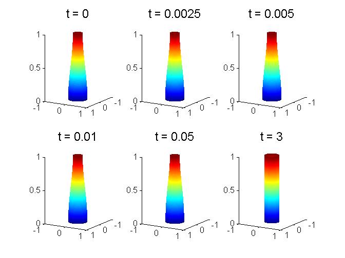
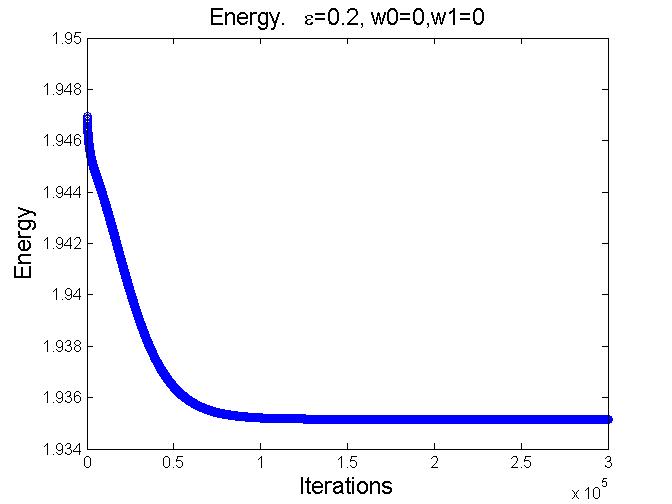
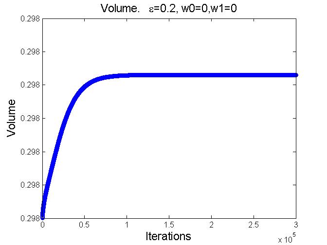
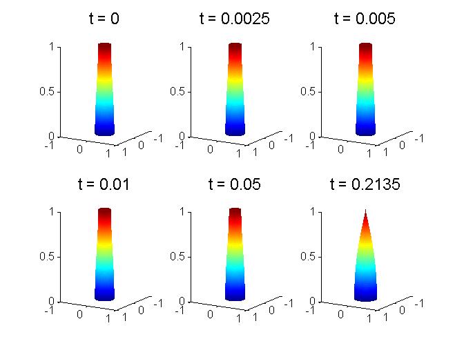
Axially symmetric volume constrained anisotropic mean curvature flow

By BBENNETT PALMER and WENXIANG ZHU
Abstract

We study the long time existence theory for a non local flow associated to a free boundary problem for a trapped non liquid drop. The drop has free boundary components on two horizontal plates and its free energy is anisotropic and axially symmetric. For axially symmetric initial surfaces with sufficiently large volume, we show that the flow exists for all time.

Numerical simulations of the curvature flow are presented.

1 Introduction

The evolution of interfaces of structured materials is of interest in a wide range of disiplines related to materials science [14]. Structured materials such as crystals, polycrystals and liquid crystals have a surface energy which is anisotropic; their energy density depends on the direction of the surface at each point. Over the years, various methods have been developed to track these interfaces, including the phase-field and level set methods. Here, we will consider a particular free boundary problem utilizing the anisotropic mean curvature flow.

The mean (isotropic) curvature flow with constrained volume was considered in [9]. In relation to the free boundary problem considered here, the papers of Athanassenas [3], [4] are particularly relevant . Also, in the recent paper [5], volume preserving mean curvature flow in a Riemannian setting is studied.

Volume constrained anisotropic mean curvature flow for hypersurfaces was considered in [1], [13]. In these papers, the emphasis is on the evolution of closed convex hypersurfaces.

Consider an anisotropic surface energy which assigns to a sufficiently smooth surface with unit normal ฮฝ๐œˆ\nu the value

(1) โ„ฑโ€‹(ฮฃ)=โˆซฮฃฮณโ€‹(ฮฝ)โ€‹๐‘‘ฮฃ.โ„ฑฮฃsubscriptฮฃ๐›พ๐œˆdifferential-dฮฃ{\cal F}(\Sigma)=\int_{\Sigma}\gamma(\nu)\>d\Sigma\>.

The function ฮณ:S2โ†’๐‘+:๐›พโ†’superscript๐‘†2superscript๐‘\gamma:S^{2}\rightarrow{\bf R}^{+} is assumed to satisfy a convexity condition: the surface

(2) W=โˆ‚โ‹‚nโˆˆS2{Yโ‹…nโ‰คฮณโ€‹(n)},๐‘Šsubscript๐‘›superscript๐‘†2โ‹…๐‘Œ๐‘›๐›พ๐‘›W=\partial\bigcap_{n\in S^{2}}\{Y\cdot n\leq\gamma(n)\}\>,

which is known as the Wulff shape . In this paper, it will be assumed that

  1. (W1)

    W๐‘ŠW is a smooth,uniformly convex surface of revolution with vertical rotation axis.

  2. (W2)

    W๐‘ŠW is symmetric with respect to reflection through the horizontal plane z=0๐‘ง0z=0.

Although we will not assume it in general, the following condition will also enter into discussion.

  1. (W3)

    The generating curve of W๐‘ŠW has non-decreasing curvature (with respect to the inward pointing normal) as a function of arc length on {zโ‰ฅ0}๐‘ง0\{z\geq 0\} as one moves in an upward direction.

The condition (W3) will be referred to as the curvature condition.

Because of (W1), the Gauss map of W๐‘ŠW defines a bijection of W๐‘ŠW onto S2superscript๐‘†2S^{2}. Therefore quantities defined on W๐‘ŠW can be expressed unambiguously on the sphere. In particular, the principal curvatures of W๐‘ŠW with respect to the inward pointing normal, ฮผisubscript๐œ‡๐‘–\mu_{i}, i=1,2๐‘–12i=1,2 along the latitudinal and longitudinal directions, are given respectively by

1/ฮผ2=ฮณโˆ’ฮฝ3โ€‹ฮณโ€ฒ,1/ฮผ1=(1โˆ’ฮฝ32)โ€‹ฮณโ€ฒโ€ฒ+1/ฮผ2.formulae-sequence1subscript๐œ‡2๐›พsubscript๐œˆ3superscript๐›พโ€ฒ1subscript๐œ‡11superscriptsubscript๐œˆ32superscript๐›พโ€ฒโ€ฒ1subscript๐œ‡21/\mu_{2}=\gamma-\nu_{3}\gamma^{\prime}\>,\qquad 1/\mu_{1}=(1-\nu_{3}^{2})\gamma^{\prime\prime}+1/\mu_{2}\>.

The uniform convexity means that ฮผi>0subscript๐œ‡๐‘–0\mu_{i}>0 holds. Moreover, the position vector ฮพ1subscript๐œ‰1\xi_{1} on W๐‘ŠW can be expressed in terms of the position vector ฮฝ๐œˆ\nu on S2superscript๐‘†2S^{2} as

(3) ฮพ1=1ฮผ2โ€‹ฮฝ+ฮณโ€ฒโ€‹(ฮฝ3)โ€‹E3.subscript๐œ‰11subscript๐œ‡2๐œˆsuperscript๐›พโ€ฒsubscript๐œˆ3subscript๐ธ3\xi_{1}=\frac{1}{\mu_{2}}\nu+\gamma^{\prime}(\nu_{3})E_{3}\>.

Given an oriented embedded surface X:ฮฃโ†’๐‘3:๐‘‹โ†’ฮฃsuperscript๐‘3X:\Sigma\rightarrow{\bf R}^{3} with unit normal field ฮฝ๐œˆ\nu, we define the Cahn-Hoffman field as the composition ฮพ:=ฮพ1โˆ˜ฮฝassign๐œ‰subscript๐œ‰1๐œˆ\xi:=\xi_{1}\circ\nu. The first variation of energy defines the anisotropic mean curvature ฮ›ฮ›\Lambda by

(4) ฮดโ€‹โ„ฑ=โˆ’โˆซฮฃฮ›โ€‹ฮดโ€‹Xโ‹…ฮฝโ€‹๐‘‘ฮฃ+โˆฎโˆ‚ฮฃ(ฮพร—ฮดโ€‹Xโ‹…dโ€‹X).๐›ฟโ„ฑsubscriptฮฃโ‹…ฮ›๐›ฟ๐‘‹๐œˆdifferential-dฮฃsubscriptcontour-integralฮฃโ‹…๐œ‰๐›ฟ๐‘‹๐‘‘๐‘‹\delta{\cal F}=-\int_{\Sigma}\Lambda\delta X\cdot\nu\>d\Sigma+\oint_{\partial\Sigma}(\xi\times\delta X\cdot dX).

Some local expressions for the anisotropic mean curvature are:

ฮ›:=โˆ’traceฮฃโ€‹Aโ€‹dโ€‹ฮฝ=โˆ’(โˆ‡โ‹…Dโ€‹ฮณโˆ’2โ€‹Hโ€‹ฮณ),A:=dโ€‹ฮพ1=(D2โ€‹ฮณ+ฮณโ€‹1)|S2.formulae-sequenceassignฮ›subscripttraceฮฃ๐ด๐‘‘๐œˆโ‹…โˆ‡๐ท๐›พ2๐ป๐›พassign๐ด๐‘‘subscript๐œ‰1evaluated-atsuperscript๐ท2๐›พ๐›พ1superscript๐‘†2\Lambda:=-{\rm trace}_{\Sigma}Ad\nu=-(\nabla\cdot D\gamma-2H\gamma),\quad A:=d\xi_{1}=(D^{2}\gamma+\gamma 1)|_{S^{2}}\>.

Here D๐ทD, D2superscript๐ท2D^{2} denote the gradient and Hessian operators acting on functions on S2superscript๐‘†2S^{2}. These can always be identified with tensors on ฮฃฮฃ\Sigma by parallel translation in ๐‘3superscript๐‘3{\bf R}^{3} since Tpโ€‹ฮฃ=Tฮฝโ€‹(p)โ€‹S2subscript๐‘‡๐‘ฮฃsubscript๐‘‡๐œˆ๐‘superscript๐‘†2T_{p}\Sigma=T_{\nu(p)}S^{2}. Another useful expression is

ฮ›=โˆ’โˆ‡โ‹…ฮพ,ฮ›โ‹…โˆ‡๐œ‰\Lambda=-\nabla\cdot\xi\>,

where โˆ‡โ‹…\nabla\cdot denotes the surface divergence.

The problem we consider here is to understand the evolution to equilibrium of a drop of material trapped between two horizontal planes ฮ isubscriptฮ ๐‘–\Pi_{i}, i=0,1๐‘–01i=0,1 located at heights z=0๐‘ง0z=0 and z=h๐‘งโ„Žz=h respectively. The surface energy is assumed to be of the form (1). It will also be assumed that:

  • โ€ข

    the initial surface is axially symmetric,

  • โ€ข

    the generating curve of the initial surface is a graph over the rotation axis.

  • โ€ข

    throughout the evolution, the surfaces meets the planes ฮ isubscriptฮ ๐‘–\Pi_{i} orthogonally.

  • โ€ข

    the initial surface extends smoothly to an infinite periodic surface with period hโ„Žh.

Of course, the third assumption is a consequence of the fourth, but we include it for clarity.

It is easy to see that the axial symmetry is preserved by the evolution considered below. It is also consistent with the form of the known minimizer for sufficiently large volumes and neutral wetting along the interface of ฮฃฮฃ\Sigma with the planes, [11]. For small volumes, the drop must disconnect during the minimization process.

It will be shown below that if the initial volume is sufficiently large, then the generating curves of the evolving surfaces are also graphs for all times for which the flow is defined.

Although we expect that a similar analysis can be carried out in arbitrary dimensions, we have decided to concentrate on the case of surfaces in ๐‘3superscript๐‘3{\bf R}^{3} because of its obvious physical significance.

2 Preliminary results

We will restrict our attention to axially symmetric surfaces with vertical rotation axis. In addition, the generating curve will always be a graph of the form r=rโ€‹(z)๐‘Ÿ๐‘Ÿ๐‘งr=r(z) and we write the surface as X=(rโ€‹(z)โ€‹eiโ€‹ฮธ,z)๐‘‹๐‘Ÿ๐‘งsuperscript๐‘’๐‘–๐œƒ๐‘งX=(r(z)e^{i\theta},z) where we have identified the first two coordinates on ๐‘3superscript๐‘3{\bf R}^{3} with the complex plane ๐‚๐‚{\bf C}. The outward pointing normal to the surface is ฮฝ=(1+rz2)โˆ’1/2โ€‹(eiโ€‹ฮธ,โˆ’rz)๐œˆsuperscript1superscriptsubscript๐‘Ÿ๐‘ง212superscript๐‘’๐‘–๐œƒsubscript๐‘Ÿ๐‘ง\nu=(1+r_{z}^{2})^{-1/2}(e^{i\theta},-r_{z}).

Consider the flow:

(5) โˆ‚Xโˆ‚t=(ฮ›โˆ’ฮ›ยฏ)โ€‹ฮฝ,๐‘‹๐‘กฮ›ยฏฮ›๐œˆ\frac{\partial X}{\partial t}=(\Lambda-{\bar{\Lambda}})\nu\>,

with the boundary condition

(6) ฮฝโ‹…E3โ‰ก0,onโ€‹โˆ‚ฮฃ.โ‹…๐œˆsubscript๐ธ30onฮฃ\nu\cdot E_{3}\equiv 0\>,\>{\rm on}\>\partial\Sigma\>.

From (14), we obtain

(7) โˆ‚tz=(ฮ›โˆ’ฮ›ยฏ)โ€‹ฮฝ3.subscript๐‘ก๐‘งฮ›ยฏฮ›subscript๐œˆ3\partial_{t}z=(\Lambda-{\bar{\Lambda}})\>\nu_{3}\>.

It is evident from this formula that, in general, z๐‘งz must depend on t๐‘กt, so, following [7], we write z=zโ€‹(ฮถ,t)๐‘ง๐‘ง๐œ๐‘กz=z(\zeta,t) where we choose ฮถ๐œ\zeta to lie in the interval [0,h]0โ„Ž[0,h]. We then express the immersion as

X=Xโ€‹(ฮถ,t)=(rโ€‹(zโ€‹(ฮถ,t),t),zโ€‹(ฮถ,t)).๐‘‹๐‘‹๐œ๐‘ก๐‘Ÿ๐‘ง๐œ๐‘ก๐‘ก๐‘ง๐œ๐‘กX=X(\zeta,t)=(r(z(\zeta,t),t),z(\zeta,t))\>.

We get

rzโ€‹zt+rt=(ฮ›โˆ’ฮ›ยฏ)โ€‹1โˆ’ฮฝ32subscript๐‘Ÿ๐‘งsubscript๐‘ง๐‘กsubscript๐‘Ÿ๐‘กฮ›ยฏฮ›1superscriptsubscript๐œˆ32r_{z}z_{t}+r_{t}=(\Lambda-{\bar{\Lambda}})\sqrt{1-\nu_{3}^{2}}\>

Combining this with (7), we get, using that ฮฝ3=โˆ’rz/1+rz2subscript๐œˆ3subscript๐‘Ÿ๐‘ง1superscriptsubscript๐‘Ÿ๐‘ง2\nu_{3}=-r_{z}/\sqrt{1+r_{z}^{2}},

rt=(ฮ›โˆ’ฮ›ยฏ)โ€‹(1โˆ’ฮฝ32โˆ’rzโ€‹ฮฝ3)=(ฮ›โˆ’ฮ›ยฏ)โ€‹(11+rz2+rz21+rz2),subscript๐‘Ÿ๐‘กฮ›ยฏฮ›1superscriptsubscript๐œˆ32subscript๐‘Ÿ๐‘งsubscript๐œˆ3ฮ›ยฏฮ›11superscriptsubscript๐‘Ÿ๐‘ง2superscriptsubscript๐‘Ÿ๐‘ง21superscriptsubscript๐‘Ÿ๐‘ง2r_{t}=(\Lambda-{\bar{\Lambda}})(\sqrt{1-\nu_{3}^{2}}-r_{z}\nu_{3})=(\Lambda-{\bar{\Lambda}})(\frac{1}{\sqrt{1+r_{z}^{2}}}+\frac{r_{z}^{2}}{\sqrt{1+r_{z}^{2}}})\>,

i.e.

(8) rt=(ฮ›โˆ’ฮ›ยฏ)โ€‹1+rz2.subscript๐‘Ÿ๐‘กฮ›ยฏฮ›1superscriptsubscript๐‘Ÿ๐‘ง2r_{t}=(\Lambda-{\bar{\Lambda}})\sqrt{1+r_{z}^{2}}\>.

The evolution for r๐‘Ÿr is identical with the evolution for r๐‘Ÿr under the flow

(โˆ‚tX)โŸ‚=(ฮ›โˆ’ฮ›0)โ€‹ฮฝ,superscriptsubscript๐‘ก๐‘‹perpendicular-toฮ›subscriptฮ›0๐œˆ(\partial_{t}X)^{\perp}=(\Lambda-\Lambda_{0})\nu\>,

where โŸ‚perpendicular-to\perp denotes the normal component.

Short time existence for (8) is standard, see for example Theorem 8.1.1 of [12]. By the equation (12), (13) given below, both ฮ›ฮ›\Lambda and ฮ›ยฏยฏฮ›{\bar{\Lambda}} are expressible in terms of r๐‘Ÿr and its derivatives.

The admissible variations for the variational problem are those which keep the surface between the planes, ฮดโ€‹Xโ‹…E3โ‰ก0โ‹…๐›ฟ๐‘‹subscript๐ธ30\delta X\cdot E_{3}\equiv 0 on โˆ‚ฮฃฮฃ\partial\Sigma , and fix the three dimensional volume enclosed within the surface:

โˆซฮฃฮดโ€‹Xโ‹…ฮฝโ€‹๐‘‘ฮฃ=0.subscriptฮฃโ‹…๐›ฟ๐‘‹๐œˆdifferential-dฮฃ0\int_{\Sigma}\delta X\cdot\nu\>d\Sigma=0\>.

The infinitesimal generator (ฮ›โˆ’ฮ›ยฏ)โ€‹ฮฝฮ›ยฏฮ›๐œˆ(\Lambda-{\bar{\Lambda}})\nu of the evolution (5), (6) clearly satisfies these conditions.

By (6), along โˆ‚ฮฃฮฃ\partial\Sigma, the normal ฮฝ๐œˆ\nu is contained in the horizontal equator of S2superscript๐‘†2S^{2}. By (W2), ฮณโ€ฒโ€‹(ฮฝ3=0)=0superscript๐›พโ€ฒsubscript๐œˆ300\gamma^{\prime}(\nu_{3}=0)=0 holds and so by (3), ฮพ๐œ‰\xi and Xtsubscript๐‘‹๐‘กX_{t} are parallel along โˆ‚ฮฃฮฃ\partial\Sigma. we then get from the first variation formula (4),

โˆ‚tโ„ฑโ€‹[ฮฃt]=โˆ’โˆซฮฃฮ›โ€‹(ฮ›โˆ’ฮ›ยฏ)โ€‹๐‘‘ฮฃ=โˆ’โˆซฮฃ(ฮ›โˆ’ฮ›ยฏ)2โ€‹๐‘‘ฮฃ,subscript๐‘กโ„ฑdelimited-[]subscriptฮฃ๐‘กsubscriptฮฃฮ›ฮ›ยฏฮ›differential-dฮฃsubscriptฮฃsuperscriptฮ›ยฏฮ›2differential-dฮฃ\partial_{t}{\cal F}[\Sigma_{t}]=-\int_{\Sigma}\Lambda(\Lambda-{\bar{\Lambda}})\>d\Sigma=-\int_{\Sigma}(\Lambda-{\bar{\Lambda}})^{2}\>d\Sigma\>,

so the flow decreases the anisotropic energy.
Remark When the wetting is not neutral, it appears to be problematic to construct an analogous flow. In this case, the boundary condition for the minimizer ฮพโ‹…E3โ‰กciโ‰ 0โ‹…๐œ‰subscript๐ธ3subscript๐‘๐‘–0\xi\cdot E_{3}\equiv c_{i}\neq 0 on โˆ‚ฮฃโˆฉฮ iฮฃsubscriptฮ ๐‘–\partial\Sigma\cap\Pi_{i}, where cisubscript๐‘๐‘–c_{i} are non zero constants related to the coupling constants for the wetting energy. This boundary condition is incompatible with the flow given by (5) maintaining the drop between the planes .

For the boundary value problem we are considering, the morphology of the minimizer depends the initial volume and whether or not the condition (W3) holds. If (W3) holds, it was shown in [11] that for volumes greater than or equal to a critical value V0subscript๐‘‰0V_{0}, all stable equilibria must be cylinders. Below this value, any minimizer must either disconnect or loose contact with at least one of the supporting planes.

When (W3) does not hold, numerical simulations for a particular class of functionals, [2], show that anisotropic unduloids may occur as stable equilibria for a certain range of volumes. However, for large volumes, only cylinders occur and for sufficiently small volumes, there is no stable connected surface spanning the two supporting planes.

We will next show that of the initial volume is sufficiently large, the surfaces will not pinch off, i.e. the generating curves are bounded away from the rotation axis.

The following lemma uses calibrations to show a minimizing property of graphs with ฮ›=0ฮ›0\Lambda=0. It is well known and its proof is given for completeness.

Lemma 2.1.

Let ฮฃฮฃ\Sigma be a surface with zero anisotropic mean curvature which can be represented as a graph over a planar domain ฮฉฮฉ\Omega. Let S๐‘†S be a piecewise smooth oriented surface which is contained in the cylinder ฮฉร—๐‘ฮฉ๐‘\Omega\times{\bf R} and which has the same boundary as ฮฃฮฃ\Sigma. Then,

โ„ฑโ€‹[ฮฃ]โ‰คโ„ฑโ€‹[S]โ„ฑdelimited-[]ฮฃโ„ฑdelimited-[]๐‘†{\cal F}[\Sigma]\leq{\cal F}[S]\>

holds.

Remark. In saying that ฮฃฮฃ\Sigma and S๐‘†S share the same boundary, we mean that ฮฃโˆ’Sฮฃ๐‘†\Sigma-S is the oriented boundary of an oriented 3-chain.
Proof. Let ฮพ๐œ‰\xi denote the Cahn-Hoffman field of ฮฃฮฃ\Sigma. The condition that ฮฃฮฃ\Sigma has zero anisotropic mean curvature is expressed โˆ‡โ‹…ฮพ=0โ‹…โˆ‡๐œ‰0\nabla\cdot\xi=0.

Because ฮฃฮฃ\Sigma is a graph, we can extend ฮพ๐œ‰\xi to a field ฮพ~~๐œ‰{\tilde{\xi}} on ฮฉร—๐‘ฮฉ๐‘\Omega\times{\bf R} by making ฮพ~~๐œ‰{\tilde{\xi}} constant on all vertical lines through points in ฮฉฮฉ\Omega. This field will satisfy โˆ‡~โ‹…ฮพ~โ‹…~โˆ‡~๐œ‰{\tilde{\nabla}}\cdot{\tilde{\xi}}, where โˆ‡~~โˆ‡{\tilde{\nabla}} denotes the divergence operator on ๐‘3superscript๐‘3{\bf R}^{3}. Then, by the Stokesโ€™ Theorem, we get

โ„ฑโ€‹[ฮฃ]โ„ฑdelimited-[]ฮฃ\displaystyle{\cal F}[\Sigma] =\displaystyle= โˆซฮฃฮณโ€‹(ฮฝฮฃ)โ€‹๐‘‘ฮฃ=โˆซฮฃฮพโ‹…ฮฝฮฃโ€‹๐‘‘ฮฃsubscriptฮฃ๐›พsubscript๐œˆฮฃdifferential-dฮฃsubscriptฮฃโ‹…๐œ‰subscript๐œˆฮฃdifferential-dฮฃ\displaystyle\int_{\Sigma}\gamma(\nu_{\Sigma})\>d\Sigma=\int_{\Sigma}\xi\cdot\nu_{\Sigma}d\Sigma
=\displaystyle= โˆซฮฃฮพ~โ‹…ฮฝฮฃโ€‹๐‘‘ฮฃ=โˆซSฮพ~โ‹…ฮฝSโ€‹๐‘‘Ssubscriptฮฃโ‹…~๐œ‰subscript๐œˆฮฃdifferential-dฮฃsubscript๐‘†โ‹…~๐œ‰subscript๐œˆ๐‘†differential-d๐‘†\displaystyle\int_{\Sigma}{\tilde{\xi}}\cdot\nu_{\Sigma}\>d\Sigma=\int_{S}{\tilde{\xi}}\cdot\nu_{S}\>dS
โ‰ค\displaystyle\leq โˆซSฮณโ€‹(ฮฝS)โ€‹๐‘‘S=โ„ฑโ€‹[S],subscript๐‘†๐›พsubscript๐œˆ๐‘†differential-d๐‘†โ„ฑdelimited-[]๐‘†\displaystyle\int_{S}\gamma(\nu_{S})\>dS={\cal F}[S]\>,

where the inequality follows from (2).

Corollary 2.1.

Let โ„ฑโ„ฑ{\cal F} be an axially symmetric anisotropic surface energy and let CโŠ‚ฮ i๐ถsubscriptฮ ๐‘–C\subset\Pi_{i} be a circle. Let S๐‘†S be any piecewise smooth compact surface bounded by C๐ถC and which is contained in the cylinder over the disc bounded by C๐ถC. Also, let D๐ทD be the flat disc bounded by C๐ถC. Then

โ„ฑโ€‹[S]โ‰ฅโ„ฑโ€‹[D]=ฮณโ€‹(e3)โ€‹|D|โ„ฑdelimited-[]๐‘†โ„ฑdelimited-[]๐ท๐›พsubscript๐‘’3๐ท{\cal F}[S]\geq{\cal F}[D]=\gamma(e_{3})|D|\>

holds.

Proof. This follows immediately from the previous lemma using the fact that the disc has zero anisotropic mean curvature.

Proposition 2.1.

Let ฮฃ0subscriptฮฃ0\Sigma_{0} be an initial axially symmetric surface enclosing a volume V๐‘‰V and intersecting the supporting planes orthogonally. Assume that

(9) โ„ฑโ€‹[ฮฃ0]<ฮณโ€‹(e3)โ€‹Vโ€‹[ฮฃ0]dโ„ฑdelimited-[]subscriptฮฃ0๐›พsubscript๐‘’3๐‘‰delimited-[]subscriptฮฃ0๐‘‘{\cal F}[\Sigma_{0}]<\gamma(e_{3})\frac{V[\Sigma_{0}]}{d}\>

holds and that the flow (5) exists for all tโˆˆ[0,T)๐‘ก0๐‘‡t\in[0,T). Then, then no pinching occurs. In particular

(10) rโ‰ฅc0๐‘Ÿsubscript๐‘0r\geq c_{0}\>

holds for tโˆˆ[0,T)๐‘ก0๐‘‡t\in[0,T), where

ฮณ(e3)Vโ€‹[ฮฃ0]dโˆ’โ„ฑ[ฮฃ0]=:ฯ€c02.\gamma(e_{3})\frac{V[\Sigma_{0}]}{d}-{\cal F}[\Sigma_{0}]=:\pi c_{0}^{2}\>.

Proof. Recall that โ„ฑโ€‹[ฮฃt]โ„ฑdelimited-[]subscriptฮฃ๐‘ก{\cal F}[\Sigma_{t}] is non increasing. Let C๐ถC denote the cylinder between ฮ 0subscriptฮ 0\Pi_{0} and ฮ 1subscriptฮ 1\Pi_{1} enclosing the same volume Vโ€‹[ฮฃ0]๐‘‰delimited-[]subscriptฮฃ0V[\Sigma_{0}] as ฮฃ0subscriptฮฃ0\Sigma_{0}. Let rCsubscript๐‘Ÿ๐ถr_{C} be the radius of this cylinder. If ฯ:=rโ€‹(ฮถ,t1)<c0assign๐œŒ๐‘Ÿ๐œsubscript๐‘ก1subscript๐‘0\rho:=r(\zeta,t_{1})<c_{0} for some t1<Tsubscript๐‘ก1๐‘‡t_{1}<T and some ฮถ๐œ\zeta, we can find an annular part of the surface ฮฃt1subscriptฮฃsubscript๐‘ก1\Sigma_{t_{1}} bounded by two circles of radii ฯ๐œŒ\rho and radius rt1>rCsubscript๐‘Ÿsubscript๐‘ก1subscript๐‘Ÿ๐ถr_{t_{1}}>r_{C}. From this piece of ฮฃt1subscriptฮฃsubscript๐‘ก1\Sigma_{t_{1}}, we form a piecewise smooth disc type surface by filling the circle of radius ฯ๐œŒ\rho with a disc.

By the previous corollary, we obtain

โ„ฑโ€‹[ฮฃ0]+ฯ€โ€‹c02>โ„ฑโ€‹[ฮฃt1]+ฯ€โ€‹ฯ2>ฮณโ€‹(e3)โ€‹ฯ€โ€‹rt12โ‰ฅฮณโ€‹(e3)โ€‹ฯ€โ€‹rc2=ฮณโ€‹(e3)โ€‹Vโ€‹(ฮฃ0)d,โ„ฑdelimited-[]subscriptฮฃ0๐œ‹superscriptsubscript๐‘02โ„ฑdelimited-[]subscriptฮฃsubscript๐‘ก1๐œ‹superscript๐œŒ2๐›พsubscript๐‘’3๐œ‹superscriptsubscript๐‘Ÿsubscript๐‘ก12๐›พsubscript๐‘’3๐œ‹superscriptsubscript๐‘Ÿ๐‘2๐›พsubscript๐‘’3๐‘‰subscriptฮฃ0๐‘‘{\cal F}[\Sigma_{0}]+\pi c_{0}^{2}>{\cal F}[\Sigma_{t_{1}}]+\pi\rho^{2}>\gamma(e_{3})\pi r_{t_{1}}^{2}\geq\gamma(e_{3})\pi r_{c}^{2}=\gamma(e_{3})\frac{V(\Sigma_{0})}{d}\>,

which gives a contradiction.

Lemma 2.2.

Assume the conditions (W1), (W2) hold for W๐‘ŠW and that ฮฃฮฃ\Sigma is an axially symmetric surface intersecting the planes ฮ isubscriptฮ ๐‘–\Pi_{i} orthogonally for which (10) holds. Then there exists c1=c1โ€‹(c0)subscript๐‘1subscript๐‘1subscript๐‘0c_{1}=c_{1}(c_{0}) such that

c1โ‰ฅ|ฮ›ยฏ|subscript๐‘1ยฏฮ›c_{1}\geq|{\bar{\Lambda}}|

holds. If, in addition (W3) holds, then we have

0โ‰ฅฮ›ยฏโ‰ฅc1>โˆ’โˆž.0ยฏฮ›subscript๐‘10\geq{\bar{\Lambda}}\geq c_{1}>-\infty\>.

Proof. The idea of the proof is essentially taken from [3].

We first note that the curvature condition (W3) can be expressed

(11) ฮฝ3โ€‹โˆ‚ฮฝ3ฮผ1โ‰ฅ0,โˆ€ฮฝ3.subscript๐œˆ3subscriptsubscript๐œˆ3subscript๐œ‡10for-allsubscript๐œˆ3\nu_{3}\partial_{\nu_{3}}\mu_{1}\geq 0,\>\forall\nu_{3}\>.

For an axially symmetric surface whose generating curve is a graph, the anisotropic mean curvature is given by

(12) ฮ›=k1ฮผ1+k2ฮผ2=rzโ€‹zฮผ1โ€‹(1+rz2)3/2โˆ’1ฮผ2โ€‹rโ€‹(1+rz2)1/2.ฮ›subscript๐‘˜1subscript๐œ‡1subscript๐‘˜2subscript๐œ‡2subscript๐‘Ÿ๐‘ง๐‘งsubscript๐œ‡1superscript1superscriptsubscript๐‘Ÿ๐‘ง2321subscript๐œ‡2๐‘Ÿsuperscript1superscriptsubscript๐‘Ÿ๐‘ง212\Lambda=\frac{k_{1}}{\mu_{1}}+\frac{k_{2}}{\mu_{2}}=\frac{r_{zz}}{\mu_{1}(1+r_{z}^{2})^{3/2}}-\frac{1}{\mu_{2}r(1+r_{z}^{2})^{1/2}}\>.

and its average value is

(13) ฮ›ยฏ=โˆซ0hฮ›โ€‹rโ€‹(1+rz2)1/2โ€‹๐‘‘zโˆซ0hrโ€‹(1+rz2)1/2โ€‹๐‘‘z.ยฏฮ›superscriptsubscript0โ„Žฮ›๐‘Ÿsuperscript1superscriptsubscript๐‘Ÿ๐‘ง212differential-d๐‘งsuperscriptsubscript0โ„Ž๐‘Ÿsuperscript1superscriptsubscript๐‘Ÿ๐‘ง212differential-d๐‘ง{\bar{\Lambda}}=\frac{\int_{0}^{h}\Lambda r(1+r_{z}^{2})^{1/2}\>dz}{\int_{0}^{h}r(1+r_{z}^{2})^{1/2}\>dz}\>.

Recall that ฮผisubscript๐œ‡๐‘–\mu_{i} are the principal curvatures of the Wulff shape W๐‘ŠW with respect to the inward pointing normal so 0<<ฮผi<โˆžmuch-less-than0subscript๐œ‡๐‘–0<<\mu_{i}<\infty holds. It then follows easily that

0โ‰ฅโˆซ0hk2ฮผ2โ€‹rโ€‹(1+rz2)1/2โ€‹๐‘‘zโˆซ0hrโ€‹(1+rz2)1/2โ€‹๐‘‘z=โˆซ0hโˆ’1ฮผ2โ€‹๐‘‘zโˆซ0hrโ€‹(1+rz2)1/2โ€‹๐‘‘zโ‰ฅc2โ€‹(c0).0superscriptsubscript0โ„Žsubscript๐‘˜2subscript๐œ‡2๐‘Ÿsuperscript1superscriptsubscript๐‘Ÿ๐‘ง212differential-d๐‘งsuperscriptsubscript0โ„Ž๐‘Ÿsuperscript1superscriptsubscript๐‘Ÿ๐‘ง212differential-d๐‘งsuperscriptsubscript0โ„Ž1subscript๐œ‡2differential-d๐‘งsuperscriptsubscript0โ„Ž๐‘Ÿsuperscript1superscriptsubscript๐‘Ÿ๐‘ง212differential-d๐‘งsubscript๐‘2subscript๐‘00\geq\frac{\int_{0}^{h}\frac{k_{2}}{\mu_{2}}r(1+r_{z}^{2})^{1/2}\>dz}{\int_{0}^{h}r(1+r_{z}^{2})^{1/2}\>dz}=\frac{\int_{0}^{h}\frac{-1}{\mu_{2}}\>dz}{\int_{0}^{h}r(1+r_{z}^{2})^{1/2}\>dz}\geq c_{2}(c_{0})\>.

From the boundary condition, we have rz=0subscript๐‘Ÿ๐‘ง0r_{z}=0 on โˆ‚ฮฃ0subscriptฮฃ0\partial\Sigma_{0}. Note that rzโ€‹z/(1+rz2)=(arctanโกrz)zsubscript๐‘Ÿ๐‘ง๐‘ง1superscriptsubscript๐‘Ÿ๐‘ง2subscriptsubscript๐‘Ÿ๐‘ง๐‘งr_{zz}/(1+r_{z}^{2})=(\arctan r_{z})_{z}. We get

โˆซฮฃk1ฮผ1โ€‹๐‘‘ฮฃsubscriptฮฃsubscript๐‘˜1subscript๐œ‡1differential-dฮฃ\displaystyle\int_{\Sigma}\frac{k_{1}}{\mu_{1}}\>d\Sigma =\displaystyle= 2โ€‹ฯ€โ€‹โˆซ0hrโ€‹rzโ€‹zฮผ1โ€‹(1+rz2)โ€‹๐‘‘z2๐œ‹superscriptsubscript0โ„Ž๐‘Ÿsubscript๐‘Ÿ๐‘ง๐‘งsubscript๐œ‡11superscriptsubscript๐‘Ÿ๐‘ง2differential-d๐‘ง\displaystyle 2\pi\int_{0}^{h}\frac{rr_{zz}}{\mu_{1}(1+r_{z}^{2})}\>dz
=\displaystyle= 2โ€‹ฯ€โ€‹โˆซ0hrฮผ1โ€‹(arctanโกrz)zโ€‹๐‘‘z2๐œ‹superscriptsubscript0โ„Ž๐‘Ÿsubscript๐œ‡1subscriptsubscript๐‘Ÿ๐‘ง๐‘งdifferential-d๐‘ง\displaystyle 2\pi\int_{0}^{h}\frac{r}{\mu_{1}}(\arctan r_{z})_{z}\>dz
=\displaystyle= โˆ’2โ€‹ฯ€โ€‹โˆซ0hrzฮผ1โ€‹(arctanโกrz)โ€‹๐‘‘zโˆ’2โ€‹ฯ€โ€‹โˆซ0hโˆ‚z(1ฮผ1)โ€‹rโ€‹(arctanโกrz)โ€‹dโ€‹z.2๐œ‹superscriptsubscript0โ„Žsubscript๐‘Ÿ๐‘งsubscript๐œ‡1subscript๐‘Ÿ๐‘งdifferential-d๐‘ง2๐œ‹superscriptsubscript0โ„Žsubscript๐‘ง1subscript๐œ‡1๐‘Ÿsubscript๐‘Ÿ๐‘ง๐‘‘๐‘ง\displaystyle-2\pi\int_{0}^{h}\frac{r_{z}}{\mu_{1}}(\arctan r_{z})\>dz-2\pi\int_{0}^{h}\partial_{z}(\frac{1}{\mu_{1}})r(\arctan r_{z})\>dz\>.

Note that, using Proposition (2.1), we obtain

0โ‰ฅโˆ’2โ€‹ฯ€โ€‹โˆซ0hrzฮผ1โ€‹(arctanโกrz)โ€‹๐‘‘z2โ€‹ฯ€โ€‹โˆซ0hrโ€‹(1+rz2)1/2โ€‹๐‘‘zโ‰ฅc3โ€‹(c0).02๐œ‹superscriptsubscript0โ„Žsubscript๐‘Ÿ๐‘งsubscript๐œ‡1subscript๐‘Ÿ๐‘งdifferential-d๐‘ง2๐œ‹superscriptsubscript0โ„Ž๐‘Ÿsuperscript1superscriptsubscript๐‘Ÿ๐‘ง212differential-d๐‘งsubscript๐‘3subscript๐‘00\geq\frac{-2\pi\int_{0}^{h}\frac{r_{z}}{\mu_{1}}(\arctan r_{z})\>dz}{2\pi\int_{0}^{h}r(1+r_{z}^{2})^{1/2}\>dz}\geq c_{3}(c_{0})\>.

First assume that (W3) holds. Note that since ฮฝ3=โˆ’rz/1+rz2subscript๐œˆ3subscript๐‘Ÿ๐‘ง1superscriptsubscript๐‘Ÿ๐‘ง2\nu_{3}=-r_{z}/\sqrt{1+r_{z}^{2}}, we can write

โˆ’2โ€‹ฯ€โ€‹โˆซโˆ‚z(1ฮผ1)โ€‹rโ€‹(arctanโกrz)โ€‹dโ€‹z2๐œ‹subscript๐‘ง1subscript๐œ‡1๐‘Ÿsubscript๐‘Ÿ๐‘ง๐‘‘๐‘ง\displaystyle-2\pi\int\partial_{z}(\frac{1}{\mu_{1}})r(\arctan r_{z})\>dz =\displaystyle= โˆ’2โ€‹ฯ€โ€‹โˆซโˆ‚ฮฝ3(1ฮผ1)โ€‹rโ€‹(arctanโก(โˆ’ฮฝ31โˆ’ฮฝ32))โ€‹dโ€‹ฮฝ32๐œ‹subscriptsubscript๐œˆ31subscript๐œ‡1๐‘Ÿsubscript๐œˆ31superscriptsubscript๐œˆ32๐‘‘subscript๐œˆ3\displaystyle-2\pi\int\partial_{\nu_{3}}(\frac{1}{\mu_{1}})r(\arctan\bigl{(}\frac{-\nu_{3}}{\sqrt{1-\nu_{3}^{2}}}\bigr{)})\>d\nu_{3}
=\displaystyle= โˆ’2โ€‹ฯ€โ€‹โˆซ(โˆ‚ฮฝ3ฮผ1ฮผ12)โ€‹rโ€‹(arctanโก(ฮฝ31โˆ’ฮฝ32))โ€‹๐‘‘ฮฝ32๐œ‹subscriptsubscript๐œˆ3subscript๐œ‡1subscriptsuperscript๐œ‡21๐‘Ÿsubscript๐œˆ31superscriptsubscript๐œˆ32differential-dsubscript๐œˆ3\displaystyle-2\pi\int(\frac{\partial_{\nu_{3}}\mu_{1}}{\mu^{2}_{1}})r(\arctan\bigl{(}\frac{\nu_{3}}{\sqrt{1-\nu_{3}^{2}}}\bigr{)})\>d\nu_{3}
โ‰ค\displaystyle\leq 00\displaystyle 0\>

by (11), since ฮฝ3subscript๐œˆ3\nu_{3} and arctanโก(ฮฝ3โ€‹(1โˆ’ฮฝ32)โˆ’1/2)subscript๐œˆ3superscript1superscriptsubscript๐œˆ3212\arctan(\nu_{3}(1-\nu_{3}^{2})^{-1/2}) have the same sign. Also, since โˆ‚ฮฝ3ฮผ1/ฮผ12subscriptsubscript๐œˆ3subscript๐œ‡1superscriptsubscript๐œ‡12\partial_{\nu_{3}}\mu_{1}/\mu_{1}^{2} is uniformly bounded, we obtain that

0โ‰ฅโˆซฮฃk1ฮผ1โ€‹๐‘‘ฮฃโˆซฮฃ๐‘‘ฮฃโ‰ฅc4โ€‹(c0),0subscriptฮฃsubscript๐‘˜1subscript๐œ‡1differential-dฮฃsubscriptฮฃdifferential-dฮฃsubscript๐‘4subscript๐‘00\geq\frac{\int_{\Sigma}\frac{k_{1}}{\mu_{1}}\>d\Sigma}{\int_{\Sigma}\>d\Sigma}\geq c_{4}(c_{0})\>,

and the result follows by combining this with the previous inequalities.

It (W3) is not assumed to hold, then we easily obtain |(k1/ฮผ1)|โ€‹dโ€‹ฮฃโ‰คcโ€‹rโ€‹dโ€‹zโ€‹dโ€‹ฮธsubscript๐‘˜1subscript๐œ‡1๐‘‘ฮฃ๐‘๐‘Ÿ๐‘‘๐‘ง๐‘‘๐œƒ|(k_{1}/\mu_{1})|\>d\Sigma\leq cr\>dz\>d\theta for a constant c๐‘c while the integrand in the denominator is counded below by r๐‘Ÿr. q.e.d

3 Evolution equations

Again, the governing evolution equation is

(14) โˆ‚tX=(ฮ›โˆ’ฮ›ยฏ)โ€‹ฮฝ.subscript๐‘ก๐‘‹ฮ›ยฏฮ›๐œˆ\partial_{t}X=(\Lambda-{\bar{\Lambda}})\>\nu\>.

For any smooth variation ฮดโ€‹X=ฯˆโ€‹ฮฝ+T๐›ฟ๐‘‹๐œ“๐œˆ๐‘‡\delta X=\psi\nu+T of a surface X๐‘‹X, the corresponding pointwise variation of the anisotropic mean curvature is

(15) ฮดโ€‹ฮ›=Jโ€‹[ฯˆ]+โˆ‡ฮ›โ‹…T.๐›ฟฮ›๐ฝdelimited-[]๐œ“โˆ‡โ‹…ฮ›๐‘‡\delta\Lambda=J[\psi]+\nabla\Lambda\cdot T\>.

Here J๐ฝJ is the self=adjoint elliptic operator given by

(16) Jโ€‹[u]=โˆ‡โ‹…Aโ€‹โˆ‡u+โŸจAโ€‹dโ€‹ฮฝ,dโ€‹ฮฝโŸฉโ€‹u.๐ฝdelimited-[]๐‘ขโ‹…โˆ‡๐ดโˆ‡๐‘ข๐ด๐‘‘๐œˆ๐‘‘๐œˆ๐‘ขJ[u]=\nabla\cdot A\nabla u+\langle Ad\nu,d\nu\rangle u\>.

Using that the evolution of X๐‘‹X is given by (5), we obtain

(17) ฮ›tโˆ’โˆ‡โ‹…Aโ€‹โˆ‡ฮ›=โŸจdโ€‹ฮฝ,Aโ€‹dโ€‹ฮฝโŸฉโ€‹(ฮ›โˆ’ฮ›ยฏ).subscriptฮ›๐‘กโ‹…โˆ‡๐ดโˆ‡ฮ›๐‘‘๐œˆ๐ด๐‘‘๐œˆฮ›ยฏฮ›\Lambda_{t}-\nabla\cdot A\nabla\Lambda=\langle d\nu,Ad\nu\rangle(\Lambda-{\bar{\Lambda}})\>.

We recall from [11] that the normal ฮฝ๐œˆ\nu satisfies the equation

(18) โˆ‡โ‹…Aโ€‹โˆ‡ฮฝj+โŸจAโ€‹dโ€‹ฮฝ,dโ€‹ฮฝโŸฉโ€‹ฮฝj=โˆ’โˆ‡ฮ›โ‹…Ej,j=1,2,3.formulae-sequenceโ‹…โˆ‡๐ดโˆ‡subscript๐œˆ๐‘—๐ด๐‘‘๐œˆ๐‘‘๐œˆsubscript๐œˆ๐‘—โˆ‡โ‹…ฮ›subscript๐ธ๐‘—๐‘—123\nabla\cdot A\nabla\nu_{j}+\langle Ad\nu,d\nu\rangle\nu_{j}=-\nabla\Lambda\cdot E_{j}\>,\>j=1,2,3\>.

This is a consequence of (15) and the translation invariance of the functional.

To compute the evolution of the normal, we use that for ฮดโ€‹X=ฯˆโ€‹ฮฝ+T๐›ฟ๐‘‹๐œ“๐œˆ๐‘‡\delta X=\psi\nu+T, one has ฮดโ€‹ฮฝ=โˆ’โˆ‡ฯˆ+dโ€‹ฮฝโ€‹T๐›ฟ๐œˆโˆ‡๐œ“๐‘‘๐œˆ๐‘‡\delta\nu=-\nabla\psi+d\nu T. Since Xt=(ฮ›โˆ’ฮ›ยฏ)โ€‹ฮฝsubscript๐‘‹๐‘กฮ›ยฏฮ›๐œˆX_{t}=(\Lambda-{\bar{\Lambda}})\nu, we get

(19) ฮฝt=โˆ’โˆ‡ฮ›subscript๐œˆ๐‘กโˆ‡ฮ›\nu_{t}=-\nabla\Lambda

We define the parabolic operator

Pโ€‹[f]=ftโˆ’โˆ‡โ‹…Aโ€‹โˆ‡f.๐‘ƒdelimited-[]๐‘“subscript๐‘“๐‘กโ‹…โˆ‡๐ดโˆ‡๐‘“P[f]=f_{t}-\nabla\cdot A\nabla f\>.
Lemma 3.1.

Define ฯ‰:=1+rz2=1/1โˆ’ฮฝ32assign๐œ”1superscriptsubscript๐‘Ÿ๐‘ง211superscriptsubscript๐œˆ32\omega:=\sqrt{1+r_{z}^{2}}=1/\sqrt{1-\nu_{3}^{2}}\>. Then

(20) Pโ€‹[ฯ‰]=โˆ’2โ€‹โˆ‡ฯ‰โ‹…Aโ€‹โˆ‡ฯ‰ฯ‰+ฯ‰r2โ€‹ฮผ2โˆ’โŸจAโ€‹dโ€‹ฮฝ,dโ€‹ฮฝโŸฉโ€‹ฯ‰.๐‘ƒdelimited-[]๐œ”2โˆ‡โ‹…๐œ”๐ดโˆ‡๐œ”๐œ”๐œ”superscript๐‘Ÿ2subscript๐œ‡2๐ด๐‘‘๐œˆ๐‘‘๐œˆ๐œ”P[\omega]=\frac{-2\nabla\omega\cdot A\nabla\omega}{\omega}+\frac{\omega}{r^{2}\mu_{2}}-\langle A\>d\nu,d\nu\rangle\omega\>.

Proof. By combining (18) and (19), we obtain the vector equation

Pโ€‹[ฮฝ]=โˆ’โˆ‡ฮ›.๐‘ƒdelimited-[]๐œˆโˆ‡ฮ›P[\nu]=-\nabla\Lambda\>.

For the surface of revolution, we have

ฮฝ=(1โˆ’ฮฝ32โ€‹eiโ€‹ฮธ,ฮฝ3),๐œˆ1superscriptsubscript๐œˆ32superscript๐‘’๐‘–๐œƒsubscript๐œˆ3\nu=(\sqrt{1-\nu_{3}^{2}}\>e^{i\theta},\nu_{3})\>,

where we have identified the space of the first two coordinates with the complex plane. It follows from (18) that

(21) โˆ‡โ‹…Aโˆ‡(1โˆ’ฮฝ32)eiโ€‹ฮธ)=โˆ’โŸจdฮฝ,AdฮฝโŸฉ(1โˆ’ฮฝ32eiโ€‹ฮธโˆ’โˆ‡ฮ›ยฏ,\nabla\cdot A\nabla(\sqrt{1-\nu_{3}^{2}}\,)e^{i\theta})=-\langle d\nu,Ad\nu\rangle(\sqrt{1-\nu_{3}^{2}}e^{i\theta}-\underline{\nabla\Lambda}\>,

where the last term denotes the projection of โˆ‡ฮ›โˆ‡ฮ›\nabla\Lambda onto ๐‘2superscript๐‘2{\bf R}^{2}.

The metric on ฮฃฮฃ\Sigma is dโ€‹S2=(1+rz2)โ€‹dโ€‹z2+r2โ€‹dโ€‹ฮธ2:=ฮฑ1โŠ—ฮฑ1+ฮฑ2โŠ—ฮฑ2๐‘‘superscript๐‘†21superscriptsubscript๐‘Ÿ๐‘ง2๐‘‘superscript๐‘ง2superscript๐‘Ÿ2๐‘‘superscript๐œƒ2assigntensor-productsubscript๐›ผ1subscript๐›ผ1tensor-productsubscript๐›ผ2subscript๐›ผ2dS^{2}=(1+r_{z}^{2})dz^{2}+r^{2}d\theta^{2}:=\alpha_{1}\otimes\alpha_{1}+\alpha_{2}\otimes\alpha_{2} If fโ€‹(z)๐‘“๐‘งf(z) is a differentiable function, then โˆ‡fโ‹…โˆ‡ฮธdฮฃ=dfโˆงโˆ—dฮธ=fzdzโˆงโˆ—ฮฑ2/r=fzdzโˆง(โˆ’ฯ‰/r)dz=0\nabla f\cdot\nabla\theta d\Sigma=df\wedge*d\theta=f_{z}dz\wedge*\alpha_{2}/r=f_{z}dz\wedge(-\omega/r)dz=0, and therefore โˆ‡fโ‹…โˆ‡ฮธ=0โ‹…โˆ‡๐‘“โˆ‡๐œƒ0\nabla f\cdot\nabla\theta=0. Also ฮ”โ€‹ฮธโ€‹dโ€‹S=dโˆ—dโ€‹ฮธ=dโˆ—(ฮฑ2/r)=dโ€‹(โˆ’ฯ‰/r)โ€‹dโ€‹z=0ฮ”๐œƒ๐‘‘๐‘†๐‘‘๐‘‘๐œƒ๐‘‘subscript๐›ผ2๐‘Ÿ๐‘‘๐œ”๐‘Ÿ๐‘‘๐‘ง0\Delta\theta\>dS=d*d\theta=d*(\alpha_{2}/r)=d(-\omega/r)dz=0. Finally |โˆ‡ฮธ|2dS=dฮธโˆงโˆ—dฮธ=dฮธโˆง(โˆ’ฯ‰/r)dz=(1/r2)dฮฃ|\nabla\theta|^{2}dS=d\theta\wedge*d\theta=d\theta\wedge(-\omega/r)dz=(1/r^{2})\>d\Sigma so |โˆ‡ฮธ|2=1/r2superscriptโˆ‡๐œƒ21superscript๐‘Ÿ2|\nabla\theta|^{2}=1/r^{2}.

Using these formulas to expand out the left hand side of (21) and using that ฮฝ3subscript๐œˆ3\nu_{3} only depends on z๐‘งz, we have

โˆ‡โ‹…Aโ€‹โˆ‡(1โˆ’ฮฝ32โ€‹eiโ€‹ฮธ)=eiโ€‹ฮธโ€‹โˆ‡โ‹…Aโ€‹โˆ‡(1โˆ’ฮฝ32)+iโ€‹eiโ€‹ฮธโ€‹1โˆ’ฮฝ32ฮผ2โ€‹(iโ€‹|โˆ‡ฮธ|2+ฮ”โ€‹ฮธ)=eiโ€‹ฮธโ€‹โˆ‡โ‹…Aโ€‹โˆ‡(1โˆ’ฮฝ32)โˆ’eiโ€‹ฮธโ€‹1โˆ’ฮฝ32r2โ€‹ฮผ2.โ‹…โˆ‡๐ดโˆ‡1superscriptsubscript๐œˆ32superscript๐‘’๐‘–๐œƒabsentโ‹…superscript๐‘’๐‘–๐œƒโˆ‡๐ดโˆ‡1superscriptsubscript๐œˆ32๐‘–superscript๐‘’๐‘–๐œƒ1superscriptsubscript๐œˆ32subscript๐œ‡2๐‘–superscriptโˆ‡๐œƒ2ฮ”๐œƒabsentโ‹…superscript๐‘’๐‘–๐œƒโˆ‡๐ดโˆ‡1superscriptsubscript๐œˆ32superscript๐‘’๐‘–๐œƒ1superscriptsubscript๐œˆ32superscript๐‘Ÿ2subscript๐œ‡2\begin{array}[]{l}\displaystyle\nabla\cdot A\nabla(\sqrt{1-\nu_{3}^{2}}e^{i\theta})\\ \displaystyle\qquad=e^{i\theta}\nabla\cdot A\nabla(\sqrt{1-\nu_{3}^{2}})+ie^{i\theta}\frac{\sqrt{1-\nu_{3}^{2}}}{\mu_{2}}(i|\nabla\theta|^{2}+\Delta\theta)\\ \displaystyle\qquad=e^{i\theta}\nabla\cdot A\nabla(\sqrt{1-\nu_{3}^{2}})-e^{i\theta}\frac{\sqrt{1-\nu_{3}^{2}}}{r^{2}\mu_{2}}\>.\end{array}

Combining this with (21), we get

(22) โˆ‡โ‹…Aโ€‹โˆ‡(1โˆ’ฮฝ32)=1โˆ’ฮฝ32ฮผ2โ€‹r2โˆ’โŸจAโ€‹dโ€‹ฮฝ,dโ€‹ฮฝโŸฉโ€‹1โˆ’ฮฝ32โˆ’eโˆ’iโ€‹ฮธโ€‹โˆ‡ฮ›ยฏ.โ‹…โˆ‡๐ดโˆ‡1superscriptsubscript๐œˆ321superscriptsubscript๐œˆ32subscript๐œ‡2superscript๐‘Ÿ2๐ด๐‘‘๐œˆ๐‘‘๐œˆ1superscriptsubscript๐œˆ32superscript๐‘’๐‘–๐œƒยฏโˆ‡ฮ›\nabla\cdot A\nabla(\sqrt{1-\nu_{3}^{2}})=\frac{\sqrt{1-\nu_{3}^{2}}}{\mu_{2}r^{2}}-\langle Ad\nu,d\nu\rangle\sqrt{1-\nu_{3}^{2}}-e^{-i\theta}\underline{\nabla\Lambda}\>.

From this, it is easy to obtain

โˆ‡โ‹…Aโ€‹โˆ‡ฯ‰=โˆ‡โ‹…Aโ€‹โˆ‡11โˆ’ฮฝ32โˆ’(1โˆ’ฮฝ32)โˆ’1โ€‹โˆ‡โ‹…Aโ€‹โˆ‡(1โˆ’ฮฝ32)โˆ’โˆ‡(1โˆ’ฮฝ32)โˆ’1โ‹…Aโˆ‡1โˆ’ฮฝ32=โˆ’ฯ‰ฮผ2โ€‹r2+โŸจAdฮฝ,dฮฝโŸฉฯ‰+eโˆ’iโ€‹ฮธฯ‰2โˆ‡ฮ›ยฏโˆ’โˆ‡(1โˆ’ฮฝ32)โˆ’1โ‹…Aโˆ‡1โˆ’ฮฝ32=โˆ’ฯ‰ฮผ2โ€‹r2+โŸจAโ€‹dโ€‹ฮฝ,dโ€‹ฮฝโŸฉโ€‹ฯ‰+eโˆ’iโ€‹ฮธโ€‹ฯ‰2โ€‹โˆ‡ฮ›ยฏ+2ฯ‰โ€‹โˆ‡ฯ‰โ‹…Aโ€‹โˆ‡ฯ‰=(โˆ—).\begin{array}[]{l}\displaystyle\nabla\cdot A\nabla\omega\vphantom{\frac{1}{2}}\\ \displaystyle\qquad=\nabla\cdot A\nabla\frac{1}{\sqrt{1-\nu_{3}^{2}}}-(1-\nu_{3}^{2})^{-1}\nabla\cdot A\nabla(\sqrt{1-\nu_{3}^{2}})\\ \displaystyle\qquad\quad-\nabla(1-\nu_{3}^{2})^{-1}\cdot A\nabla\sqrt{1-\nu_{3}^{2}}\vphantom{\frac{1}{2}}\\ \displaystyle\qquad=-\frac{\omega}{\mu_{2}r^{2}}+\langle Ad\nu,d\nu\rangle\omega+e^{-i\theta}\omega^{2}\underline{\nabla\Lambda}-\nabla(1-\nu_{3}^{2})^{-1}\cdot A\nabla\sqrt{1-\nu_{3}^{2}}\\ \displaystyle\qquad=-\frac{\omega}{\mu_{2}r^{2}}+\langle Ad\nu,d\nu\rangle\omega+e^{-i\theta}\omega^{2}\underline{\nabla\Lambda}+\frac{2}{\omega}\nabla\omega\cdot A\nabla\omega\\ \displaystyle\qquad=(*)\vphantom{\frac{1}{2}}\>.\end{array}

From (19), we get (1โˆ’ฮฝ32)t=โˆ’eโˆ’iโ€‹ฮธโ€‹โˆ‡ฮ›ยฏsubscript1superscriptsubscript๐œˆ32๐‘กsuperscript๐‘’๐‘–๐œƒยฏโˆ‡ฮ›(\sqrt{1-\nu_{3}^{2}})_{t}=-e^{-i\theta}\underline{\nabla\Lambda} which implies

ฯ‰t=(1โˆ’ฮฝ32)โˆ’1โ€‹eโˆ’iโ€‹ฮธโ€‹โˆ‡ฮ›ยฏ=ฯ‰2โ€‹eโˆ’iโ€‹ฮธโ€‹โˆ‡ฮ›ยฏ.subscript๐œ”๐‘กsuperscript1superscriptsubscript๐œˆ321superscript๐‘’๐‘–๐œƒยฏโˆ‡ฮ›superscript๐œ”2superscript๐‘’๐‘–๐œƒยฏโˆ‡ฮ›\omega_{t}=(1-\nu_{3}^{2})^{-1}e^{-i\theta}\underline{\nabla\Lambda}=\omega^{2}e^{-i\theta}\underline{\nabla\Lambda}\>.

Combining this with (*) yields (20)

We state the following well known Maximum Principle, [15].

Theorem 3.1.

If the operator uโ†ฆโˆ‡โ‹…Aโ€‹โˆ‡[u]maps-to๐‘ขโ‹…โˆ‡๐ดโˆ‡๐‘ขu\mapsto\nabla\cdot A\nabla[u] is elliptic and h:Mร—[t1,t2]โ†’๐‘:โ„Žโ†’๐‘€subscript๐‘ก1subscript๐‘ก2๐‘h:M\times[t_{1},t_{2}]\rightarrow{\bf R} satisfies

(โˆ‚tโˆ’โˆ‡โ‹…Aโ€‹โˆ‡)โ€‹hโ‰ค0,subscript๐‘กโ‹…โˆ‡๐ดโˆ‡โ„Ž0(\partial_{t}-\nabla\cdot A\nabla)h\leq 0\>,

holds, then

maxMโกhโ€‹(โ‹…,t)โ‰คmaxMโกhโ€‹(โ‹…,t1).subscript๐‘€โ„Žโ‹…๐‘กsubscript๐‘€โ„Žโ‹…subscript๐‘ก1\max_{M}h(\cdot,t)\leq\max_{M}h(\cdot,t_{1})\>.

In the case we are considering, ellipticity of uโ†ฆโˆ‡โ‹…Aโ€‹โˆ‡[u]maps-to๐‘ขโ‹…โˆ‡๐ดโˆ‡๐‘ขu\mapsto\nabla\cdot A\nabla[u] follows from the convexity condition W1.

Proposition 3.1.

Assume that the initial surface satisfies the estimate (9). Then the generating curve is a graph for all time t๐‘กt for which the evolution (5) exists.

Proof. As in [3], we use the boundary condition (6) and the assumptions on the initial curve to extend the surfaces generated by the flow to periodic surfaces.

For any constant c๐‘c, we obtain from (20)

(23) (logโก(ฯ‰)โˆ’cโ€‹t)tโˆ’โˆ‡โ‹…Aโ€‹โˆ‡(logโก(ฯ‰)โˆ’cโ€‹t)=1r2โ€‹ฮผ2โˆ’cโˆ’โˆ‡ฯ‰โ‹…Aโ€‹โˆ‡ฯ‰ฯ‰2โˆ’โŸจAโ€‹dโ€‹ฮฝ,dโ€‹ฮฝโŸฉ.subscript๐œ”๐‘๐‘ก๐‘กโ‹…โˆ‡๐ดโˆ‡๐œ”๐‘๐‘ก1superscript๐‘Ÿ2subscript๐œ‡2๐‘โˆ‡โ‹…๐œ”๐ดโˆ‡๐œ”superscript๐œ”2๐ด๐‘‘๐œˆ๐‘‘๐œˆ(\log(\omega)-ct)_{t}-\nabla\cdot A\nabla(\log(\omega)-ct)=\frac{1}{r^{2}\mu_{2}}-c-\frac{\nabla\omega\cdot A\nabla\omega}{\omega^{2}}-\langle A\>d\nu,d\nu\rangle\>.

By Proposition (2.1), there is a constant c0=c0โ€‹(t1)subscript๐‘0subscript๐‘0subscript๐‘ก1c_{0}=c_{0}(t_{1}) such that rโ‰ฅc0๐‘Ÿsubscript๐‘0r\geq c_{0} holds for tโˆˆ[t,t1]๐‘ก๐‘กsubscript๐‘ก1t\in[t,t_{1}]. Hence, for a suitable constant c๐‘c, we have (logโก(ฯ‰)โˆ’cโ€‹t)tโˆ’โˆ‡โ‹…Aโ€‹โˆ‡(logโก(ฯ‰)โˆ’cโ€‹t)โ‰ค0subscript๐œ”๐‘๐‘ก๐‘กโ‹…โˆ‡๐ดโˆ‡๐œ”๐‘๐‘ก0(\log(\omega)-ct)_{t}-\nabla\cdot A\nabla(\log(\omega)-ct)\leq 0. It follows from the Maximum Principal, that

(24) max0โ‰คzโ‰คd,0โ‰คtโ‰คt1โก(logโก(ฯ‰)โˆ’cโ€‹t)โ‰คmax0โ‰คzโ‰คd,t=0โกlogโกฯ‰.subscriptformulae-sequence0๐‘ง๐‘‘0๐‘กsubscript๐‘ก1๐œ”๐‘๐‘กsubscriptformulae-sequence0๐‘ง๐‘‘๐‘ก0๐œ”\max_{0\leq z\leq d,0\leq t\leq t_{1}}(\log(\omega)-ct)\leq\max_{0\leq z\leq d,t=0}\log\omega\>.

From the definition of ฯ‰๐œ”\omega we have from (24) that there exist constants c2โ€‹(ฮฃ0)subscript๐‘2subscriptฮฃ0c_{2}(\Sigma_{0}), a2โ€‹(ฮฃ0)subscript๐‘Ž2subscriptฮฃ0a_{2}(\Sigma_{0}) such that if the flow exists for tโˆˆ[0,T)๐‘ก0๐‘‡t\in[0,T), then

(25) ฯ‰โ‰คc2โ€‹ea2โ€‹t::๐œ”subscript๐‘2superscript๐‘’subscript๐‘Ž2๐‘กabsent\omega\leq c_{2}e^{a_{2}t}:\,

for 0โ‰คt<T0๐‘ก๐‘‡0\leq t<T.

Recalling the definition of ฯ‰๐œ”\omega, the result follows. q.e.d.

Proposition 3.2.

Assume the conditions (W1) and (W2) hold. Assume that the flow (5) is defined for 0โ‰คt<T0๐‘ก๐‘‡0\leq t<T. Then the curvatures of the surfaces Xโ€‹(t)๐‘‹๐‘กX(t) remain bounded, i.e. there exists a constant c3โ€‹(T)subscript๐‘3๐‘‡c_{3}(T). with

(26) k12(t)+k22(t)=:||dฮฝ||2(t)โ‰คc3(T),โˆ€t,0โ‰คt<Tk_{1}^{2}(t)+k_{2}^{2}(t)=:||d\nu||^{2}(t)\leq c_{3}(T)\>,\forall t,0\leq t<T

where kiโ€‹(t)subscript๐‘˜๐‘–๐‘กk_{i}(t) denote the principal curvatures at time t๐‘กt.

First note that k2=โˆ’(rโ€‹ฯ‰)โˆ’1subscript๐‘˜2superscript๐‘Ÿ๐œ”1k_{2}=-(r\omega)^{-1}. By Proposition (2.1) we have rโ‰ฅc0โ€‹(T)๐‘Ÿsubscript๐‘0๐‘‡r\geq c_{0}(T) and c4โ€‹(T)โ‰ฅฯ‰โ‰ฅ1subscript๐‘4๐‘‡๐œ”1c_{4}(T)\geq\omega\geq 1 by the previous proposition and the definition of ฯ‰๐œ”\omega. It follows that |k2|โ‰คc5โ€‹(T)subscript๐‘˜2subscript๐‘5๐‘‡|k_{2}|\leq c_{5}(T). Since ฮผisubscript๐œ‡๐‘–\mu_{i}, i=1,2๐‘–12i=1,2, are uniformly bounded below and above, (0<aโ‰คฮผiโ‰ค1/a0๐‘Žsubscript๐œ‡๐‘–1๐‘Ž0<a\leq\mu_{i}\leq 1/a for some aโˆˆ๐‘๐‘Ž๐‘a\in{\bf R}), it is enough to show the existence of a bound

(27) ฮ›2โ‰คc6โ€‹(T)superscriptฮ›2subscript๐‘6๐‘‡\Lambda^{2}\leq c_{6}(T)

for 0โ‰คt<T0๐‘ก๐‘‡0\leq t<T and then (26) will follow.

We recall the standard formula:

(28) Pโ€‹[fโ€‹g]=fโ€‹Pโ€‹[g]+gโ€‹Pโ€‹[f]โˆ’2โ€‹โˆ‡fโ‹…Aโ€‹โˆ‡g,๐‘ƒdelimited-[]๐‘“๐‘”๐‘“๐‘ƒdelimited-[]๐‘”๐‘”๐‘ƒdelimited-[]๐‘“2โˆ‡โ‹…๐‘“๐ดโˆ‡๐‘”P[fg]=fP[g]+gP[f]-2\nabla f\cdot A\nabla g\>,

for sufficiently smooth functions f๐‘“f and g๐‘”g. The endomorphism field A=D2โ€‹ฮณ+ฮณโ€‹id๐ดsuperscript๐ท2๐›พ๐›พidA=D^{2}\gamma+\gamma{\rm id} is self-adjoint so that the last term is symmetric in f,g๐‘“๐‘”f,g.

From the last equation (17) and (20) we obtain

(29) Pโ€‹[ฯ‰2]=2โ€‹ฯ‰2ฮผ2โ€‹r2โˆ’2โ€‹โŸจAโ€‹dโ€‹ฮฝ,dโ€‹ฮฝโŸฉโ€‹ฯ‰2โˆ’6โ€‹โˆ‡ฯ‰โ€‹Aโ€‹โˆ‡ฯ‰,๐‘ƒdelimited-[]superscript๐œ”22superscript๐œ”2subscript๐œ‡2superscript๐‘Ÿ22๐ด๐‘‘๐œˆ๐‘‘๐œˆsuperscript๐œ”26โˆ‡๐œ”๐ดโˆ‡๐œ”P[\omega^{2}]=\frac{2\omega^{2}}{\mu_{2}r^{2}}-2\langle Ad\nu,d\nu\rangle\omega^{2}-6\nabla\omega A\nabla\omega\>,
(30) Pโ€‹[ฮ›2]=2โ€‹โŸจAโ€‹dโ€‹ฮฝ,dโ€‹ฮฝโŸฉโ€‹ฮ›โ€‹(ฮ›โˆ’ฮ›ยฏ)โˆ’2โ€‹โˆ‡ฮ›โ‹…Aโ€‹โˆ‡ฮ›.๐‘ƒdelimited-[]superscriptฮ›22๐ด๐‘‘๐œˆ๐‘‘๐œˆฮ›ฮ›ยฏฮ›2โˆ‡โ‹…ฮ›๐ดโˆ‡ฮ›P[\Lambda^{2}]=2\langle Ad\nu,d\nu\rangle\Lambda(\Lambda-{\bar{\Lambda}})-2\nabla\Lambda\cdot A\nabla\Lambda\>.

For a suitable C2superscript๐ถ2C^{2} function hโ€‹(x)โ„Ž๐‘ฅh(x) and Bโˆˆ๐‘๐ต๐‘B\in{\bf R} both of which we determine later, we get

Pโ€‹[hโ€‹(ฯ‰2)โ€‹(ฮ›2+B)]=(ฮ›2+B)โ€‹hโ€ฒโ€‹(ฯ‰2)โ€‹(2โ€‹ฯ‰2ฮผ2โ€‹r2โˆ’2โ€‹โŸจAโ€‹dโ€‹ฮฝ,dโ€‹ฮฝโŸฉโ€‹ฯ‰2โˆ’6โ€‹โˆ‡ฯ‰โ€‹Aโ€‹โˆ‡ฯ‰)โˆ’(ฮ›2+B)โ€‹hโ€ฒโ€ฒโ€‹(ฯ‰2)โ€‹โˆ‡ฯ‰2โ‹…Aโ€‹โˆ‡ฯ‰2+hโ€‹(ฯ‰2)โ€‹(2โ€‹โŸจAโ€‹dโ€‹ฮฝ,dโ€‹ฮฝโŸฉโ€‹ฮ›โ€‹(ฮ›โˆ’ฮ›ยฏ)โˆ’2โ€‹โˆ‡ฮ›โ‹…Aโ€‹โˆ‡ฮ›)โˆ’2โ€‹hโ€ฒโ€‹(ฯ‰2)โ€‹โˆ‡ฯ‰2โ‹…Aโ€‹โˆ‡ฮ›2.๐‘ƒdelimited-[]โ„Žsuperscript๐œ”2superscriptฮ›2๐ตabsentsuperscriptฮ›2๐ตsuperscriptโ„Žโ€ฒsuperscript๐œ”22superscript๐œ”2subscript๐œ‡2superscript๐‘Ÿ22๐ด๐‘‘๐œˆ๐‘‘๐œˆsuperscript๐œ”26โˆ‡๐œ”๐ดโˆ‡๐œ”superscriptฮ›2๐ตsuperscriptโ„Žโ€ฒโ€ฒsuperscript๐œ”2โˆ‡โ‹…superscript๐œ”2๐ดโˆ‡superscript๐œ”2โ„Žsuperscript๐œ”22๐ด๐‘‘๐œˆ๐‘‘๐œˆฮ›ฮ›ยฏฮ›2โˆ‡โ‹…ฮ›๐ดโˆ‡ฮ›2superscriptโ„Žโ€ฒsuperscript๐œ”2โˆ‡โ‹…superscript๐œ”2๐ดโˆ‡superscriptฮ›2\begin{array}[]{l}\displaystyle P[h(\omega^{2})(\Lambda^{2}+B)]\vphantom{\dfrac{1}{2}}\\ \displaystyle\qquad=(\Lambda^{2}+B)h^{\prime}(\omega^{2})\bigl{(}\frac{2\omega^{2}}{\mu_{2}r^{2}}-2\langle Ad\nu,d\nu\rangle\omega^{2}-6\nabla\omega A\nabla\omega\bigr{)}\\ \displaystyle\qquad\quad-\;(\Lambda^{2}+B)h^{\prime\prime}(\omega^{2})\nabla\omega^{2}\cdot A\nabla\omega^{2}\vphantom{\dfrac{1}{2}}\\ \displaystyle\qquad\quad+\;h(\omega^{2})\bigl{(}2\langle Ad\nu,d\nu\rangle\Lambda(\Lambda-{\bar{\Lambda}})-2\nabla\Lambda\cdot A\nabla\Lambda\bigr{)}-2h^{\prime}(\omega^{2})\nabla\omega^{2}\cdot A\nabla\Lambda^{2}.\vphantom{\dfrac{1}{2}}\end{array}

We take hโ€‹(x):=eaโ€‹xassignโ„Ž๐‘ฅsuperscript๐‘’๐‘Ž๐‘ฅh(x):=e^{ax} for a constant a๐‘Ža to be determined later, and get

Pโ€‹[eaโ€‹ฯ‰2โ€‹(ฮ›2+B)]=eaโ€‹ฯ‰2((ฮ›2+B)a(2โ€‹ฯ‰2ฮผ2โ€‹r2โˆ’2โŸจAdฮฝ,dฮฝโŸฉฯ‰2โˆ’6โˆ‡ฯ‰Aโˆ‡ฯ‰)โˆ’(ฮ›2+B)โ€‹a2โ€‹โˆ‡ฯ‰2โ‹…Aโ€‹โˆ‡ฯ‰2+2โ€‹โŸจAโ€‹dโ€‹ฮฝ,dโ€‹ฮฝโŸฉโ€‹ฮ›โ€‹(ฮ›โˆ’ฮ›ยฏ)โˆ’2โˆ‡ฮ›โ‹…Aโˆ‡ฮ›โˆ’2aโˆ‡ฯ‰2โ‹…Aโˆ‡ฮ›2)=eaโ€‹ฯ‰2(2โ€‹aโ€‹(ฮ›2+B)ฮผ2โ€‹r2+[โˆ’2a(ฮ›2+B)+2ฮ›2โˆ’2ฮ›ฮ›ยฏ]โŸจAdฮฝ,dฮฝโŸฉ+[โˆ’6a2(ฮ›2+B)โˆ‡ฯ‰2โ‹…Aโˆ‡ฯ‰2โˆ’2โˆ‡ฮ›โ‹…Aโˆ‡ฮ›โˆ’2aโˆ‡ฯ‰2โ‹…Aโˆ‡ฮ›2])=(โˆ—โˆ—).\begin{array}[]{l}\displaystyle P[e^{a\omega^{2}}(\Lambda^{2}+B)]\vphantom{\dfrac{1}{2}}\\ \displaystyle\qquad=e^{a\omega^{2}}\biggl{(}(\Lambda^{2}+B)a\bigl{(}\frac{2\omega^{2}}{\mu_{2}r^{2}}-2\langle Ad\nu,d\nu\rangle\omega^{2}-6\nabla\omega A\nabla\omega\bigr{)}\\ \displaystyle\qquad\quad-(\Lambda^{2}+B)a^{2}\nabla\omega^{2}\cdot A\nabla\omega^{2}+2\langle Ad\nu,d\nu\rangle\Lambda(\Lambda-{\bar{\Lambda}})\vphantom{\dfrac{1}{2}}\\ \displaystyle\qquad\quad-2\nabla\Lambda\cdot A\nabla\Lambda-2a\nabla\omega^{2}\cdot A\nabla\Lambda^{2}\biggr{)}\vphantom{\dfrac{1}{2}}\\ \displaystyle\qquad=e^{a\omega^{2}}\biggl{(}\frac{2a(\Lambda^{2}+B)}{\mu_{2}r^{2}}+\bigl{[}-2a(\Lambda^{2}+B)+2\Lambda^{2}-2\Lambda{\bar{\Lambda}}\bigr{]}\langle Ad\nu,d\nu\rangle\\ \displaystyle\qquad\quad+\bigl{[}-6a^{2}(\Lambda^{2}+B)\nabla\omega^{2}\cdot A\nabla\omega^{2}-2\nabla\Lambda\cdot A\nabla\Lambda-2a\nabla\omega^{2}\cdot A\nabla\Lambda^{2}\bigr{]}\biggr{)}\vphantom{\dfrac{1}{2}}\\ \displaystyle\qquad=(**).\end{array}

We have

โˆ’2โ€‹aโ€‹(ฮ›2+B)+2โ€‹ฮ›2โˆ’2โ€‹ฮ›โ€‹ฮ›ยฏโ‰คโˆ’2โ€‹aโ€‹(ฮ›2+B)+3โ€‹ฮ›2+ฮ›ยฏ2,2๐‘Žsuperscriptฮ›2๐ต2superscriptฮ›22ฮ›ยฏฮ›2๐‘Žsuperscriptฮ›2๐ต3superscriptฮ›2superscriptยฏฮ›2-2a(\Lambda^{2}+B)+2\Lambda^{2}-2\Lambda{\bar{\Lambda}}\leq-2a(\Lambda^{2}+B)+3\Lambda^{2}+{\bar{\Lambda}}^{2}\>,

using 2โ€‹xโ€‹yโ‰คx2+y22๐‘ฅ๐‘ฆsuperscript๐‘ฅ2superscript๐‘ฆ22xy\leq x^{2}+y^{2}. Because of Lemma (13), we have the existence of a constant c1โ€‹(T)subscript๐‘1๐‘‡c_{1}(T) with ฮ›ยฏ2โ‰ค(c1โ€‹(T))2superscriptยฏฮ›2superscriptsubscript๐‘1๐‘‡2{\bar{\Lambda}}^{2}\leq(c_{1}(T))^{2}. Hence by choosing a,B>>0much-greater-than๐‘Ž๐ต0a,B>>0, we get that the term in (**) which includes the factor โŸจAโ€‹dโ€‹ฮฝ,dโ€‹ฮฝโŸฉ๐ด๐‘‘๐œˆ๐‘‘๐œˆ\langle Ad\nu,d\nu\rangle is non positive.

Next notice that since the tensor A๐ดA is positive definite and self adjoint, at each fixed point pโˆˆฮฃ๐‘ฮฃp\in\Sigma, we have an inner product defined by (u,v)=Aโ€‹uโ‹…v๐‘ข๐‘ฃโ‹…๐ด๐‘ข๐‘ฃ(u,v)=Au\cdot v, u,vโˆˆTpโ€‹ฮฃ๐‘ข๐‘ฃsubscript๐‘‡๐‘ฮฃu,v\in T_{p}\Sigma. We then have using 2โ€‹|(u,v)|โ‰ค(u,u)+(v,v)2๐‘ข๐‘ฃ๐‘ข๐‘ข๐‘ฃ๐‘ฃ2|(u,v)|\leq(u,u)+(v,v),

2โ€‹aโ€‹|โˆ‡ฯ‰2โ‹…Aโ€‹โˆ‡ฮ›2|2๐‘Žโˆ‡โ‹…superscript๐œ”2๐ดโˆ‡superscriptฮ›2\displaystyle 2a|\nabla\omega^{2}\cdot A\nabla\Lambda^{2}| =\displaystyle= 4โ€‹aโ€‹|ฮ›|โ€‹|โˆ‡ฯ‰2โ‹…Aโ€‹โˆ‡ฮ›|4๐‘Žฮ›โˆ‡โ‹…superscript๐œ”2๐ดโˆ‡ฮ›\displaystyle 4a|\Lambda||\nabla\omega^{2}\cdot A\nabla\Lambda|
=\displaystyle= 4โ€‹aโ€‹|ฮ›||(โˆ‡ฯ‰2,โˆ‡ฮ›)conditional4๐‘Žฮ›โˆ‡superscript๐œ”2โˆ‡ฮ›\displaystyle 4a|\Lambda||(\nabla\omega^{2},\nabla\Lambda)
โ‰ค\displaystyle\leq 4โ€‹a2โ€‹ฮ›2โ€‹(โˆ‡ฯ‰2,โˆ‡ฯ‰2)+(โˆ‡ฮ›,โˆ‡ฮ›)4superscript๐‘Ž2superscriptฮ›2โˆ‡superscript๐œ”2โˆ‡superscript๐œ”2โˆ‡ฮ›โˆ‡ฮ›\displaystyle 4a^{2}\Lambda^{2}(\nabla\omega^{2},\nabla\omega^{2})+(\nabla\Lambda,\nabla\Lambda)
=\displaystyle= 4โ€‹a2โ€‹ฮ›2โ€‹โˆ‡ฯ‰2โ‹…Aโ€‹โˆ‡ฯ‰2+โˆ‡ฮ›โ‹…Aโ€‹โˆ‡ฮ›.4superscript๐‘Ž2superscriptฮ›2โˆ‡โ‹…superscript๐œ”2๐ดโˆ‡superscript๐œ”2โˆ‡โ‹…ฮ›๐ดโˆ‡ฮ›\displaystyle 4a^{2}\Lambda^{2}\nabla\omega^{2}\cdot A\nabla\omega^{2}+\nabla\Lambda\cdot A\nabla\Lambda\>.

This means that both terms in (**) between the square brackets are non positive for suitable choices of the constants a๐‘Ža and B๐ตB and so we can conclude that

Pโ€‹[eaโ€‹ฯ‰2โ€‹(ฮ›2+B)]โ‰คeaโ€‹ฯ‰2โ€‹2โ€‹aโ€‹(ฮ›2+B)ฮผ2โ€‹r2,๐‘ƒdelimited-[]superscript๐‘’๐‘Žsuperscript๐œ”2superscriptฮ›2๐ตsuperscript๐‘’๐‘Žsuperscript๐œ”22๐‘Žsuperscriptฮ›2๐ตsubscript๐œ‡2superscript๐‘Ÿ2P[e^{a\omega^{2}}(\Lambda^{2}+B)]\leq e^{a\omega^{2}}\frac{2a(\Lambda^{2}+B)}{\mu_{2}r^{2}}\>,

holds. Now recall that by Proposition (2.1), we have rโ‰ฅc0โ€‹(ฮฃ0)>0๐‘Ÿsubscript๐‘0subscriptฮฃ00r\geq c_{0}(\Sigma_{0})>0. It then follows that

Pโ€‹[eโˆ’Mโ€‹tโ€‹eaโ€‹ฯ‰2โ€‹(ฮ›2+B)]๐‘ƒdelimited-[]superscript๐‘’๐‘€๐‘กsuperscript๐‘’๐‘Žsuperscript๐œ”2superscriptฮ›2๐ต\displaystyle P[e^{-Mt}e^{a\omega^{2}}(\Lambda^{2}+B)] =\displaystyle= eโˆ’Mโ€‹tโ€‹(โˆ’Mโ€‹eaโ€‹ฯ‰2โ€‹(ฮ›2+B)+Pโ€‹[eaโ€‹ฯ‰2โ€‹(ฮ›2+B)])superscript๐‘’๐‘€๐‘ก๐‘€superscript๐‘’๐‘Žsuperscript๐œ”2superscriptฮ›2๐ต๐‘ƒdelimited-[]superscript๐‘’๐‘Žsuperscript๐œ”2superscriptฮ›2๐ต\displaystyle e^{-Mt}\biggl{(}-Me^{a\omega^{2}}(\Lambda^{2}+B)+P[e^{a\omega^{2}}(\Lambda^{2}+B)]\biggr{)}
โ‰ค\displaystyle\leq eโˆ’Mโ€‹tโ€‹(โˆ’Mโ€‹eaโ€‹ฯ‰2โ€‹(ฮ›2+B)+eaโ€‹ฯ‰2โ€‹2โ€‹aโ€‹(ฮ›2+B)ฮผ2โ€‹r2)superscript๐‘’๐‘€๐‘ก๐‘€superscript๐‘’๐‘Žsuperscript๐œ”2superscriptฮ›2๐ตsuperscript๐‘’๐‘Žsuperscript๐œ”22๐‘Žsuperscriptฮ›2๐ตsubscript๐œ‡2superscript๐‘Ÿ2\displaystyle e^{-Mt}\biggl{(}-Me^{a\omega^{2}}(\Lambda^{2}+B)+e^{a\omega^{2}}\frac{2a(\Lambda^{2}+B)}{\mu_{2}r^{2}}\biggr{)}
โ‰ค\displaystyle\leq 0,0\displaystyle 0\>,

for a sufficiently large constant M๐‘€M. Recalling from Proposition (3.1) that ฯ‰โ‰ค1+c22โ€‹(T)๐œ”1superscriptsubscript๐‘22๐‘‡\omega\leq\sqrt{1+c_{2}^{2}(T)}, we find that (27) follows from the Maximum Principle. q.e.d.

4 Higher order regularity

In this section we obtain bounds on higher order derivatives of the surface. In similar problems involving mean curvature flow, these are obtained from bounds on higher order derivatives of the second fundamental form |dโ€‹ฮฝ|2superscript๐‘‘๐œˆ2|d\nu|^{2}. In our case, a nice evolution equation for this quantity is unavailable. However, since we are only working with surfaces of revolution, we can use (30) instead to obtain the desired bounds.

Proposition 4.1.

For positive constants ฯƒm=ฯƒmโ€‹(T)subscript๐œŽ๐‘šsubscript๐œŽ๐‘š๐‘‡\sigma_{m}=\sigma_{m}(T), ฯ„m=ฯ„mโ€‹(T)subscript๐œ๐‘šsubscript๐œ๐‘š๐‘‡\tau_{m}=\tau_{m}(T), there holds

(31) Pโ€‹[|โˆ‡mฮ›|2]โ‰คโˆ’ฯƒmโ€‹|โˆ‡m+1ฮ›|2+ฯ„mโ€‹(1+|โˆ‡mฮ›|2),ฯ„m=ฯ„mโ€‹(|โˆ‡jฮ›|2),j<mformulae-sequence๐‘ƒdelimited-[]superscriptsuperscriptโˆ‡๐‘šฮ›2subscript๐œŽ๐‘šsuperscriptsuperscriptโˆ‡๐‘š1ฮ›2subscript๐œ๐‘š1superscriptsuperscriptโˆ‡๐‘šฮ›2formulae-sequencesubscript๐œ๐‘šsubscript๐œ๐‘šsuperscriptsuperscriptโˆ‡๐‘—ฮ›2๐‘—๐‘šP[|\nabla^{m}\Lambda|^{2}]\leq-\sigma_{m}|\nabla^{m+1}\Lambda|^{2}+\tau_{m}(1+|\nabla^{m}\Lambda|^{2})\>,\tau_{m}=\tau_{m}(|\nabla^{j}\Lambda|^{2})\>,j<m

for 0โ‰คtโ‰คT0๐‘ก๐‘‡0\leq t\leq T.

Lemma 4.1.

Let f=fโ€‹(s)๐‘“๐‘“๐‘ f=f(s) be a sufficiently smooth function. Then

(32) |โˆ‡mf(s)โ‰ค|โˆ‡smf(s)|2+E1,|\nabla^{m}f(s)\leq|\nabla_{s}^{m}f(s)|^{2}+E_{1}\>,

where E1subscript๐ธ1E_{1} only depends on |โˆ‡jf|superscriptโˆ‡๐‘—๐‘“|\nabla^{j}f|, jโ‰คmโˆ’1๐‘—๐‘š1j\leq m-1.

Proof. The proof is straightforward and is left to the reader.

Proof of Proposition (4.1) At a fixed time t๐‘กt, we let ฯ‰1:=dโ€‹sassignsubscript๐œ”1๐‘‘๐‘ \omega_{1}:=ds, ฯ‰2=rโ€‹dโ€‹ฮธsubscript๐œ”2๐‘Ÿ๐‘‘๐œƒ\omega_{2}=rd\theta and we write, using the summation convention,

dโ€‹ฮ›=ฮ›jโ€‹ฯ‰j,โˆ‡dโ€‹ฮ›=ฮ›jโ€‹kโ€‹ฯ‰jโ€‹ฯ‰k,โ€ฆformulae-sequence๐‘‘ฮ›subscriptฮ›๐‘—subscript๐œ”๐‘—โˆ‡๐‘‘ฮ›subscriptฮ›๐‘—๐‘˜subscript๐œ”๐‘—subscript๐œ”๐‘˜โ€ฆd\Lambda=\Lambda_{j}\omega_{j}\>,\>\>\nabla d\Lambda=\Lambda_{jk}\omega_{j}\omega_{k}\>,...

Then at any time t๐‘กt, we can write

(33) |โˆ‡mฮ›|2=|ฮ›j1โ€‹โ€ฆ.jm|2โ€‹โˆk=1..mgjkโ€‹jk,|\nabla^{m}\Lambda|^{2}=|\Lambda_{j_{1}....j_{m}}|^{2}\prod_{k=1..m}g^{j_{k}j_{k}}\>,

where, although the coframe is fixed, all quantities depend on t๐‘กt. Throughout the evolution, all the surfaces are axially symmetric, so giโ€‹i=1/giโ€‹isuperscript๐‘”๐‘–๐‘–1subscript๐‘”๐‘–๐‘–g^{ii}=1/g_{ii}. For a normal variation Xโ€‹(t)=X+tโ€‹ฯˆโ€‹ฮฝ+โ€ฆ๐‘‹๐‘ก๐‘‹๐‘ก๐œ“๐œˆโ€ฆX(t)=X+t\psi\nu+..., the first variation of the metric is โˆ‚tgiโ€‹j=โˆ’2โ€‹ฯˆโ€‹hiโ€‹jsubscript๐‘กsubscript๐‘”๐‘–๐‘—2๐œ“subscriptโ„Ž๐‘–๐‘—\partial_{t}g_{ij}=-2\psi h_{ij} where hiโ€‹jsubscriptโ„Ž๐‘–๐‘—h_{ij} are the coefficients of the second fundamental form. Since all the surfaces are axially symmetric, giโ€‹j=ฮดiโ€‹jโ€‹giโ€‹isubscript๐‘”๐‘–๐‘—subscript๐›ฟ๐‘–๐‘—subscript๐‘”๐‘–๐‘–g_{ij}=\delta_{ij}g_{ii} and hiโ€‹j=ฮดiโ€‹jโ€‹hiโ€‹isubscriptโ„Ž๐‘–๐‘—subscript๐›ฟ๐‘–๐‘—subscriptโ„Ž๐‘–๐‘–h_{ij}=\delta_{ij}h_{ii} for all t๐‘กt. Using this, we obtain from (33)

โˆ‚t|โˆ‡mฮ›|2subscript๐‘กsuperscriptsuperscriptโˆ‡๐‘šฮ›2\displaystyle\partial_{t}|\nabla^{m}\Lambda|^{2} =\displaystyle= 4โ€‹Hโ€‹(ฮ›โˆ’ฮ›ยฏ)โ€‹|โˆ‡mฮ›|2+2โ€‹ฮ›j1โ€‹โ€ฆ.jmโ€‹(โˆ‚tฮ›j1โ€‹โ€ฆ.jm)โ€‹โˆk=1..mgjkโ€‹jk\displaystyle 4H(\Lambda-{\bar{\Lambda}})|\nabla^{m}\Lambda|^{2}+2\Lambda_{j_{1}....j_{m}}(\partial_{t}\Lambda_{j_{1}....j_{m}})\prod_{k=1..m}g^{j_{k}j_{k}}
=\displaystyle= 4โ€‹Hโ€‹(ฮ›โˆ’ฮ›ยฏ)โ€‹|โˆ‡mฮ›|2+2โ€‹โŸจโˆ‡mฮ›,โˆ‡mJโ€‹[ฮ›]โŸฉ4๐ปฮ›ยฏฮ›superscriptsuperscriptโˆ‡๐‘šฮ›22superscriptโˆ‡๐‘šฮ›superscriptโˆ‡๐‘š๐ฝdelimited-[]ฮ›\displaystyle 4H(\Lambda-{\bar{\Lambda}})|\nabla^{m}\Lambda|^{2}+2\langle\nabla^{m}\Lambda,\nabla^{m}J[\Lambda]\rangle
โˆผsimilar-to\displaystyle\sim 2โ€‹โŸจโˆ‡mฮ›,โˆ‡m(โˆ‡โ‹…Aโ€‹โˆ‡ฮ›)โŸฉ,2superscriptโˆ‡๐‘šฮ›superscriptโˆ‡๐‘šโ‹…โˆ‡๐ดโˆ‡ฮ›\displaystyle 2\langle\nabla^{m}\Lambda,\nabla^{m}(\nabla\cdot A\nabla\Lambda)\rangle\>,

where โˆผsimilar-to\sim means that the quantities are equal up to terms of orders less than or equal to m๐‘šm. In the given frame, for a function fโ€‹(s)๐‘“๐‘ f(s),

(34) โˆ‡โ‹…Aโ€‹โˆ‡f=1rโ€‹ฯ‰โ€‹โˆ‚s(rโ€‹fsฮผ1).โ‹…โˆ‡๐ดโˆ‡๐‘“1๐‘Ÿ๐œ”subscript๐‘ ๐‘Ÿsubscript๐‘“๐‘ subscript๐œ‡1\nabla\cdot A\nabla f=\frac{1}{r\omega}\partial_{s}(\frac{rf_{s}}{\mu_{1}})\>.

In particular, since ฮ›ฮ›\Lambda only depends on s๐‘ s, we get

(35) โˆ‚t|โˆ‡mฮ›|2โˆผ2ฯ‰โ€‹ฮผ1โ€‹(โˆ‡smฮ›)โ€‹(โˆ‡sm+2ฮ›)+ฮฆmโ€‹(โˆ‡smฮ›)โ€‹(โˆ‡sm+1ฮ›),similar-tosubscript๐‘กsuperscriptsuperscriptโˆ‡๐‘šฮ›22๐œ”subscript๐œ‡1subscriptsuperscriptโˆ‡๐‘š๐‘ ฮ›superscriptsubscriptโˆ‡๐‘ ๐‘š2ฮ›subscriptฮฆ๐‘šsubscriptsuperscriptโˆ‡๐‘š๐‘ ฮ›superscriptsubscriptโˆ‡๐‘ ๐‘š1ฮ›\partial_{t}|\nabla^{m}\Lambda|^{2}\sim\frac{2}{\omega\mu_{1}}(\nabla^{m}_{s}\Lambda)(\nabla_{s}^{m+2}\Lambda)+\Phi_{m}(\nabla^{m}_{s}\Lambda)(\nabla_{s}^{m+1}\Lambda)\>,

for suitable functions ฮฆmsubscriptฮฆ๐‘š\Phi_{m} which are bounded by lower order derivatives.

Since |โˆ‡mฮ›|2superscriptsuperscriptโˆ‡๐‘šฮ›2|\nabla^{m}\Lambda|^{2} only depends on s๐‘ s, applying (34) gives

โˆ‡โ‹…Aโ€‹โˆ‡|โˆ‡mฮ›|2โ‹…โˆ‡๐ดโˆ‡superscriptsuperscriptโˆ‡๐‘šฮ›2\displaystyle\nabla\cdot A\nabla|\nabla^{m}\Lambda|^{2} =\displaystyle= 1rโ€‹ฯ‰โ€‹โˆ‚s(rโ€‹โˆ‚s|โˆ‡mฮ›|2ฮผ1)1๐‘Ÿ๐œ”subscript๐‘ ๐‘Ÿsubscript๐‘ superscriptsuperscriptโˆ‡๐‘šฮ›2subscript๐œ‡1\displaystyle\frac{1}{r\omega}\partial_{s}(\frac{r\partial_{s}|\nabla^{m}\Lambda|^{2}}{\mu_{1}})
=\displaystyle= 1rโ€‹ฯ‰โ€‹โˆ‚s(2โ€‹rฮผ1โ€‹โŸจโˆ‡mฮ›,โˆ‡sโˆ‡mโกฮ›โŸฉ)1๐‘Ÿ๐œ”subscript๐‘ 2๐‘Ÿsubscript๐œ‡1superscriptโˆ‡๐‘šฮ›subscriptโˆ‡๐‘ superscriptโˆ‡๐‘šฮ›\displaystyle\frac{1}{r\omega}\partial_{s}(\frac{2r}{\mu_{1}}\langle\nabla^{m}\Lambda,\nabla_{s}\nabla^{m}\Lambda\rangle)
=\displaystyle= 2ฯ‰โ€‹ฮผ1โ€‹โŸจโˆ‡mฮ›,โˆ‡sโˆ‡sโˆ‡mโกฮ›โŸฉ+2ฯ‰โ€‹ฮผ1โ€‹|โˆ‡sm+1ฮ›|22๐œ”subscript๐œ‡1superscriptโˆ‡๐‘šฮ›subscriptโˆ‡๐‘ subscriptโˆ‡๐‘ superscriptโˆ‡๐‘šฮ›2๐œ”subscript๐œ‡1superscriptsuperscriptsubscriptโˆ‡๐‘ ๐‘š1ฮ›2\displaystyle\frac{2}{\omega\mu_{1}}\langle\nabla^{m}\Lambda,\nabla_{s}\nabla_{s}\nabla^{m}\Lambda\rangle+\frac{2}{\omega\mu_{1}}|\nabla_{s}^{m+1}\Lambda|^{2}
+1rโ€‹ฯ‰โ€‹(2โ€‹rฮผ1)sโ€‹โŸจโˆ‡mฮ›,โˆ‡sโˆ‡mโกฮ›โŸฉ.1๐‘Ÿ๐œ”subscript2๐‘Ÿsubscript๐œ‡1๐‘ superscriptโˆ‡๐‘šฮ›subscriptโˆ‡๐‘ superscriptโˆ‡๐‘šฮ›\displaystyle\qquad+\frac{1}{r\omega}(\frac{2r}{\mu_{1}})_{s}\langle\nabla^{m}\Lambda,\nabla_{s}\nabla^{m}\Lambda\rangle\>.

From the last equation, (35) and Lemma 4.1, we can write

Pโ€‹[|โˆ‡mฮ›|2]โˆผโˆ’2ฯ‰โ€‹ฮผ1โ€‹|โˆ‡sm+1ฮ›|2+ฮฆ~mโ€‹โŸจโˆ‡mฮ›,โˆ‡sโˆ‡mโกฮ›โŸฉ.similar-to๐‘ƒdelimited-[]superscriptsuperscriptโˆ‡๐‘šฮ›22๐œ”subscript๐œ‡1superscriptsuperscriptsubscriptโˆ‡๐‘ ๐‘š1ฮ›2subscript~ฮฆ๐‘šsuperscriptโˆ‡๐‘šฮ›subscriptโˆ‡๐‘ superscriptโˆ‡๐‘šฮ›P[\>|\nabla^{m}\Lambda|^{2}\>]\sim-\frac{2}{\omega\mu_{1}}|\nabla_{s}^{m+1}\Lambda|^{2}+{\tilde{\Phi}}_{m}\langle\nabla^{m}\Lambda,\nabla_{s}\nabla^{m}\Lambda\rangle\>.

for a suitable function ฮฆ~msubscript~ฮฆ๐‘š{\tilde{\Phi}_{m}} which depends only on lower order derivatives. The second term can be bounded

|ฮฆ~mโŸจโˆ‡mฮ›,โˆ‡sโˆ‡mฮ›โŸฉ|โ‰คฯต22|โˆ‡sm+1ฮ›|2+ฯตโˆ’22|ฮฆ~m||2โˆ‡mฮ›|2โˆผฯต22|โˆ‡sm+1ฮ›|2.|{\tilde{\Phi}}_{m}\langle\nabla^{m}\Lambda,\nabla_{s}\nabla^{m}\Lambda\rangle|\leq\frac{\epsilon^{2}}{2}|\nabla_{s}^{m+1}\Lambda|^{2}+\frac{\epsilon^{-2}}{2}|{\tilde{\Phi}}_{m}||^{2}\nabla^{m}\Lambda|^{2}\sim\frac{\epsilon^{2}}{2}|\nabla_{s}^{m+1}\Lambda|^{2}\>.

By applying lemma (4.1), we obtain

Pโ€‹[|โˆ‡mฮ›|2]โˆผโˆ’ฯƒmโ€‹|โˆ‡sm+1ฮ›|2,similar-to๐‘ƒdelimited-[]superscriptsuperscriptโˆ‡๐‘šฮ›2subscript๐œŽ๐‘šsuperscriptsuperscriptsubscriptโˆ‡๐‘ ๐‘š1ฮ›2P[\>|\nabla^{m}\Lambda|^{2}\>]\sim-\sigma_{m}|\nabla_{s}^{m+1}\Lambda|^{2}\>,

where for suitable ฯตitalic-ฯต\epsilon, we can take, using (25),

(36) ฯƒm:=(maxโก(ฮผ1)โ€‹1+c22โ€‹(T))โˆ’1.assignsubscript๐œŽ๐‘šsuperscriptsubscript๐œ‡11superscriptsubscript๐‘22๐‘‡1\sigma_{m}:=\big{(}\max(\mu_{1})\sqrt{1+c_{2}^{2}(T)}\>\>\bigr{)}^{-1}\>.

This shows that (31) holds. q.e.d.

Theorem 4.1.

There exist constants Cmโ€‹(T)subscript๐ถ๐‘š๐‘‡C_{m}(T) such that

(37) |โˆ‡mฮ›|2โ‰คCmโ€‹(T),โˆ€t<T.formulae-sequencesuperscriptsuperscriptโˆ‡๐‘šฮ›2subscript๐ถ๐‘š๐‘‡for-all๐‘ก๐‘‡|\nabla^{m}\Lambda|^{2}\leq C_{m}(T)\>,\forall t<T\>.

Proof of Th. (4.1). Denote by Sโ€‹(m)๐‘†๐‘šS(m) the statement (37). The statement Sโ€‹(0)๐‘†0S(0) is just (27) which was shown above. We assume Sโ€‹(j)๐‘†๐‘—S(j) holds for all j<m๐‘—๐‘šj<m.

Let ฮจm:=|โˆ‡mฮ›|2assignsubscriptฮจ๐‘šsuperscriptsuperscriptโˆ‡๐‘šฮ›2\Psi_{m}:=|\nabla^{m}\Lambda|^{2}. By (28), (29) and (31), we find, for positive constants a๐‘Ža and B๐ตB

Pโ€‹[eaโ€‹ฯ‰2โ€‹(ฮจm+B)]โ‰คeaโ€‹ฯ‰2(โˆ’ฯƒmฮจm+1+ฯ„m(1+ฮจm)+(ฮจm+B)โ€‹(aโ€‹[2โ€‹ฯ‰2ฮผ2โ€‹r2โˆ’2โ€‹โŸจAโ€‹dโ€‹ฮฝ,dโ€‹ฮฝโŸฉโ€‹ฯ‰2โˆ’6โ€‹โˆ‡ฯ‰โ€‹Aโ€‹โˆ‡ฯ‰]โˆ’a2โ€‹โˆ‡ฯ‰2โ‹…Aโ€‹โˆ‡ฯ‰2)โˆ’2aโˆ‡ฮจmโ‹…Aโˆ‡ฯ‰2).\begin{array}[]{l}\displaystyle P[e^{a\omega^{2}}(\Psi_{m}+B)]\vphantom{\frac{1}{2}}\\ \displaystyle\qquad\leq e^{a\omega^{2}}\biggl{(}-\sigma_{m}\Psi_{m+1}+\tau_{m}(1+\Psi_{m})\\ \displaystyle\qquad\quad+(\Psi_{m}+B)(a\bigl{[}\frac{2\omega^{2}}{\mu_{2}r^{2}}-2\langle Ad\nu,d\nu\rangle\omega^{2}-6\nabla\omega A\nabla\omega\bigr{]}-a^{2}\nabla\omega^{2}\cdot A\nabla\omega^{2})\\ \displaystyle\qquad\quad-2a\nabla\Psi_{m}\cdot A\nabla\omega^{2}\biggr{)}\>.\end{array}

We can estimate the last term above using

2โ€‹aโ€‹|โˆ‡ฮจmโ‹…Aโ€‹โˆ‡ฯ‰2|โ‰คฯต2โ€‹ฮจm+1+ฯตโˆ’2โ€‹a2โ€‹โˆ‡ฯ‰2โ‹…Aโ€‹โˆ‡ฯ‰2.2๐‘Žโˆ‡โ‹…subscriptฮจ๐‘š๐ดโˆ‡superscript๐œ”2superscriptitalic-ฯต2subscriptฮจ๐‘š1superscriptitalic-ฯต2superscript๐‘Ž2โˆ‡โ‹…superscript๐œ”2๐ดโˆ‡superscript๐œ”22a|\nabla\Psi_{m}\cdot A\nabla\omega^{2}|\leq\epsilon^{2}\Psi_{m+1}+\epsilon^{-2}a^{2}\nabla\omega^{2}\cdot A\nabla\omega^{2}\>.

We choose ฯต<ฯƒmโ€‹(T)italic-ฯตsubscript๐œŽ๐‘š๐‘‡\epsilon<\sigma_{m}(T) and choose B>>0much-greater-than๐ต0B>>0 so that โˆ’6โ€‹Bโ€‹โˆ‡ฯ‰โ€‹Aโ€‹โˆ‡ฯ‰+ฯตโˆ’2โ€‹a2โ€‹โˆ‡ฯ‰2โ‹…Aโ€‹โˆ‡ฯ‰2<06๐ตโˆ‡๐œ”๐ดโˆ‡๐œ”superscriptitalic-ฯต2superscript๐‘Ž2โˆ‡โ‹…superscript๐œ”2๐ดโˆ‡superscript๐œ”20-6B\nabla\omega A\nabla\omega+\epsilon^{-2}a^{2}\nabla\omega^{2}\cdot A\nabla\omega^{2}<0 holds. This is possible since ฯ‰๐œ”\omega is bounded by (25). Recalling that (ฯ‰/r)๐œ”๐‘Ÿ(\omega/r) is also bounded in any finite time interval, so we arrive at

Pโ€‹[eaโ€‹ฯ‰2โ€‹(ฮจm+B)]<Cโ€‹eaโ€‹ฯ‰2โ€‹(ฮจm+B),๐‘ƒdelimited-[]superscript๐‘’๐‘Žsuperscript๐œ”2subscriptฮจ๐‘š๐ต๐ถsuperscript๐‘’๐‘Žsuperscript๐œ”2subscriptฮจ๐‘š๐ตP[e^{a\omega^{2}}(\Psi_{m}+B)]<Ce^{a\omega^{2}}(\Psi_{m}+B)\>,

for tโ‰คT๐‘ก๐‘‡t\leq T and a suitable constant C=Cโ€‹(T)๐ถ๐ถ๐‘‡C=C(T). Here we are using the induction hypothesis since the constant ฯ„m=ฯ„mโ€‹(|โˆ‡jฮ›|2)subscript๐œ๐‘šsubscript๐œ๐‘šsuperscriptsuperscriptโˆ‡๐‘—ฮ›2\tau_{m}=\tau_{m}(|\nabla^{j}\Lambda|^{2}), j<m๐‘—๐‘šj<m, have been absorbed into the costant Cโ€‹(T)๐ถ๐‘‡C(T). It then follows that

Pโ€‹[eโˆ’Cโ€‹tโ€‹eaโ€‹ฯ‰2โ€‹(ฮจm+B)]<0๐‘ƒdelimited-[]superscript๐‘’๐ถ๐‘กsuperscript๐‘’๐‘Žsuperscript๐œ”2subscriptฮจ๐‘š๐ต0P[e^{-Ct}e^{a\omega^{2}}(\Psi_{m}+B)]<0\>

holds for 0โ‰คtโ‰คT0๐‘ก๐‘‡0\leq t\leq T, so the result follows from the Maximum Principle. q.e.d.

Proposition 4.2.

If (37) holds then for suitable constants, the principal curvatures satisfy

(38) |โˆ‡mk1|โ‰คcm,|โˆ‡mk2|โ‰คcmโ€ฒformulae-sequencesuperscriptโˆ‡๐‘šsubscript๐‘˜1subscript๐‘๐‘šsuperscriptโˆ‡๐‘šsubscript๐‘˜2superscriptsubscript๐‘๐‘šโ€ฒ|\nabla^{m}k_{1}|\leq c_{m}\>,\quad|\nabla^{m}k_{2}|\leq c_{m}^{\prime}

hold.

Proof. For a surface of revolution, the Codazzi equations reduce to

(k2)s=(k1โˆ’k2)โ€‹rs/r.subscriptsubscript๐‘˜2๐‘ subscript๐‘˜1subscript๐‘˜2subscript๐‘Ÿ๐‘ ๐‘Ÿ(k_{2})_{s}=(k_{1}-k_{2})r_{s}/r\>.

It follows by an easy induction argument that an upper bound for |โˆ‡smk2|subscriptsuperscriptโˆ‡๐‘š๐‘ subscript๐‘˜2|\nabla^{m}_{s}k_{2}| and hence |โˆ‡mk2|superscriptโˆ‡๐‘šsubscript๐‘˜2|\nabla^{m}k_{2}|, can be obtained from upper bounds on |โˆ‡jki|superscriptโˆ‡๐‘—subscript๐‘˜๐‘–|\nabla^{j}k_{i}|, i=1,2๐‘–12i=1,2, j<m๐‘—๐‘šj<m. For this one needs (10) and the fact that derivatives of r๐‘Ÿr of order j๐‘—j have upper bounds which depend on derivatives of k1subscript๐‘˜1k_{1} of order โ‰คjโˆ’2absent๐‘—2\leq j-2 since rsโ€‹s=k1โ€‹zssubscript๐‘Ÿ๐‘ ๐‘ subscript๐‘˜1subscript๐‘ง๐‘ r_{ss}=k_{1}z_{s}.

For a surface of revolution, the anisotropic principal curvatures are the functions ฮปj:=kj/ฮผjassignsubscript๐œ†๐‘—subscript๐‘˜๐‘—subscript๐œ‡๐‘—\lambda_{j}:=k_{j}/\mu_{j}, j=1,2๐‘—12j=1,2. These are the eigenvalues of the differential dโ€‹ฮพ:Tโ€‹ฮฃโ†’Tโ€‹W:๐‘‘๐œ‰โ†’๐‘‡ฮฃ๐‘‡๐‘Šd\xi:T\Sigma\rightarrow TW. Note that ฮ›=ฮป1+ฮป2ฮ›subscript๐œ†1subscript๐œ†2\Lambda=\lambda_{1}+\lambda_{2}.

We have (kj)s=(ฮปj)sโ€‹ฮผj+ฮปjโ€‹ฮผjโ€ฒโ€‹(ฮฝ)3โ€‹(โˆ’k1)โ€‹zssubscriptsubscript๐‘˜๐‘—๐‘ subscriptsubscript๐œ†๐‘—๐‘ subscript๐œ‡๐‘—subscript๐œ†๐‘—superscriptsubscript๐œ‡๐‘—โ€ฒsubscript๐œˆ3subscript๐‘˜1subscript๐‘ง๐‘ (k_{j})_{s}=(\lambda_{j})_{s}\mu_{j}+\lambda_{j}\mu_{j}^{\prime}(\nu)_{3}(-k_{1})z_{s} from which it follows easily that

|โˆ‡smkj|โ‰ค(maxโกฮผj)โ€‹|โˆ‡smฮปj|+E2,subscriptsuperscriptโˆ‡๐‘š๐‘ subscript๐‘˜๐‘—subscript๐œ‡๐‘—subscriptsuperscriptโˆ‡๐‘š๐‘ subscript๐œ†๐‘—subscript๐ธ2|\nabla^{m}_{s}k_{j}|\leq(\max\mu_{j})|\nabla^{m}_{s}\lambda_{j}|+E_{2}\>,
|โˆ‡smฮปj|โ‰ค(maxโก(1/ฮผj))โ€‹|โˆ‡smkj|+E2โ€ฒ,subscriptsuperscriptโˆ‡๐‘š๐‘ subscript๐œ†๐‘—1subscript๐œ‡๐‘—subscriptsuperscriptโˆ‡๐‘š๐‘ subscript๐‘˜๐‘—subscriptsuperscript๐ธโ€ฒ2|\nabla^{m}_{s}\lambda_{j}|\leq(\max(1/\mu_{j}))|\nabla^{m}_{s}k_{j}|+E^{\prime}_{2}\>,

where E2,E2โ€ฒsubscript๐ธ2superscriptsubscript๐ธ2โ€ฒE_{2},E_{2}^{\prime} depends on derivatives of the kjsubscript๐‘˜๐‘—k_{j}โ€™s of order less than or equal to mโˆ’1๐‘š1m-1.

Finally, we have from the definition of ฮ›ฮ›\Lambda,

|โˆ‡mฮป1|superscriptโˆ‡๐‘šsubscript๐œ†1\displaystyle|\nabla^{m}\lambda_{1}| โ‰ค\displaystyle\leq |โˆ‡mฮ›|+|โˆ‡mฮป2|superscriptโˆ‡๐‘šฮ›superscriptโˆ‡๐‘šsubscript๐œ†2\displaystyle|\nabla^{m}\Lambda|+|\nabla^{m}\lambda_{2}|
โ‰ค\displaystyle\leq |โˆ‡mฮ›|+(maxโก(1/ฮผj))โ€‹|โˆ‡smk2|+E2โ€ฒsuperscriptโˆ‡๐‘šฮ›1subscript๐œ‡๐‘—subscriptsuperscriptโˆ‡๐‘š๐‘ subscript๐‘˜2subscriptsuperscript๐ธโ€ฒ2\displaystyle|\nabla^{m}\Lambda|+(\max(1/\mu_{j}))|\nabla^{m}_{s}k_{2}|+E^{\prime}_{2}
โ‰ค\displaystyle\leq |โˆ‡mฮ›|+E3+E2โ€ฒ,superscriptโˆ‡๐‘šฮ›subscript๐ธ3superscriptsubscript๐ธ2โ€ฒ\displaystyle|\nabla^{m}\Lambda|+E_{3}+E_{2}^{\prime}\>,

where E3subscript๐ธ3E_{3} (and E2โ€ฒsuperscriptsubscript๐ธ2โ€ฒE_{2}^{\prime}) only depends on |โˆ‡jki|superscriptโˆ‡๐‘—subscript๐‘˜๐‘–|\nabla^{j}k_{i}|, jโ‰คmโˆ’1๐‘—๐‘š1j\leq m-1. Using induction, (37) and (26), the result follows. q.e.d.

Theorem 4.2.

Assume that the initial surface satisfies (9). Then the flow exists for all time.

Proof. The result follows by a standard argument. Assume the flow exists on a finite time interval [0,Tmax)0subscript๐‘‡max[0,T_{\rm max}). Because of the uniform estimates given by (26) and (38), the flow can also be extended smoothly to t=Tmax๐‘กsubscript๐‘‡maxt=T_{\rm max}. Then, by applying the local existence result, the flow can be extended to [0,Tmax+ฯต)0subscript๐‘‡maxitalic-ฯต[0,T_{\rm max}+\epsilon) for some ฯต>0italic-ฯต0\epsilon>0. q.e.d.

Remark We show L2superscript๐ฟ2L^{2} convergence of the anisotropic mean curvature to its mean. Note that

โˆ‚tโ„ฑโ€‹[ฮฃt]=โˆ’โˆซฮฃ(ฮ›โˆ’ฮ›ยฏ)2โ€‹๐‘‘ฮฃ,subscript๐‘กโ„ฑdelimited-[]subscriptฮฃ๐‘กsubscriptฮฃsuperscriptฮ›ยฏฮ›2differential-dฮฃ\partial_{t}{\cal F}[\Sigma_{t}]=-\int_{\Sigma}(\Lambda-{\bar{\Lambda}})^{2}\>d\Sigma\>,

and therefore

โ„ฑโ€‹[ฮฃ0]โ‰ฅโˆซ0โˆžโˆซฮฃt(ฮ›โˆ’ฮ›ยฏ)2โ€‹๐‘‘ฮฃtโ€‹๐‘‘t.โ„ฑdelimited-[]subscriptฮฃ0superscriptsubscript0subscriptsubscriptฮฃ๐‘กsuperscriptฮ›ยฏฮ›2differential-dsubscriptฮฃ๐‘กdifferential-d๐‘ก{\cal F}[\Sigma_{0}]\geq\int_{0}^{\infty}\int_{\Sigma_{t}}(\Lambda-{\bar{\Lambda}})^{2}\>d\Sigma_{t}\>dt\>.

In particular

โˆซฮฃ(ฮ›โˆ’ฮ›ยฏ)2โ€‹๐‘‘ฮฃtโ†’0,โ†’subscriptฮฃsuperscriptฮ›ยฏฮ›2differential-dsubscriptฮฃ๐‘ก0\int_{\Sigma}(\Lambda-{\bar{\Lambda}})^{2}\>d\Sigma_{t}\rightarrow 0\>,

as tโ†’โˆžโ†’๐‘กt\rightarrow\infty.

5 Numerical Results

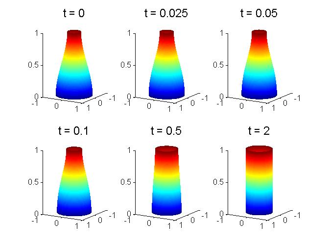
Based on the different descriptions of the evolving surface, different methods can be used to numerically solve a surface evolution equation. These include parametric, level set, and phase field methods (see [6]). Each method has its own advantage and disadvantage. We choose the parametric method, which basically is a front tracking method, namely, the surface is evolved and tracked according to the surface evolution equation (8).

Instead of using fully implicit schemes for the temporal discretization of equation (8), a semiโ€“implicit backward Euler method is used. The key of time forwarding in the semiโ€“implicit scheme is to approximate the nonlinear terms in the equation by using the previously computed approximated solution, while the linear terms still need to be solved implicitly. Therefore we can avoid solving systems of nonlinear equations (for example, using the Newtonโ€™s method) at each time step and thus the computational cost can be reduced. On the other hand, the implicit feature will increase the stability of the scheme so the restrictions on time step sizes can be loosened.

As for the spatial discretization, a secondโ€“order finite difference method can be used. Finite element method using piecewise linear functions can also be used, and if the mass is lumped, it will be equivalent to the finite difference method. However, based on our numerical experiments with the above two methods, we choose to present the method of using cubic spline approximations. The spline approximation not only provides a higher order method, it also ensures the continuity of the second order derivatives across the spatial nodes, which we think it is important in the approximation of curvature flows. On the other hand, since the curvature flow we study here is essentially one dimensional, as we will see below, when using the spline approximation, the resulting linear system that we need to solve is very sparse and the computational cost will be of the same order as the cost using finite difference or finite element method.

5.1 Approximation by Splines

In this section, we discuss numerical methods for simulating the initial boundary value problem (5) and (6). For a representative class of examples, we concentrate on the Rapiniโ€“Papoular functionals given by ฮณ=1+ฯตโ€‹ฮฝ32๐›พ1italic-ฯตsuperscriptsubscript๐œˆ32\gamma=1+\epsilon\nu_{3}^{2}, where โˆ’1โ‰คฯตโ‰ค11italic-ฯต1-1\leq\epsilon\leq 1.

We use the clamped cubic spline approximation to numerically solve the evolution equation. Let T>0๐‘‡0T>0 and let N,K๐‘๐พN,K be positive integers. Let 0=z1โ‰คโ‹ฏโ‰คzNโ‰คzN+1=10subscript๐‘ง1โ‹ฏsubscript๐‘ง๐‘subscript๐‘ง๐‘110=z_{1}\leq\cdots\leq z_{N}\leq z_{N+1}=1 be a partition of the interval [0,1]01[0,1] and let 0=t0โ‰คโ‹ฏโ‰คtKโ‰ค=T0=t_{0}\leq\cdots\leq t_{K}\leq=T be an equally spaced partition of the time interval [0,T]0๐‘‡[0,T].

We use the following notation

rnk=rโ€‹(tk,zn),(rz)nk=rzโ€‹(tk,zn),(rzโ€‹z)nk=rzโ€‹zโ€‹(tk,zn),ฮ›ยฏnk=ฮ›ยฏโ€‹(tk,zn),formulae-sequencesuperscriptsubscript๐‘Ÿ๐‘›๐‘˜๐‘Ÿsubscript๐‘ก๐‘˜subscript๐‘ง๐‘›formulae-sequencesuperscriptsubscriptsubscript๐‘Ÿ๐‘ง๐‘›๐‘˜subscript๐‘Ÿ๐‘งsubscript๐‘ก๐‘˜subscript๐‘ง๐‘›formulae-sequencesuperscriptsubscriptsubscript๐‘Ÿ๐‘ง๐‘ง๐‘›๐‘˜subscript๐‘Ÿ๐‘ง๐‘งsubscript๐‘ก๐‘˜subscript๐‘ง๐‘›superscriptsubscriptยฏฮ›๐‘›๐‘˜ยฏฮ›subscript๐‘ก๐‘˜subscript๐‘ง๐‘›\displaystyle r_{n}^{k}=r(t_{k},z_{n}),\quad(r_{z})_{n}^{k}=r_{z}(t_{k},z_{n}),\quad(r_{zz})_{n}^{k}=r_{zz}(t_{k},z_{n}),\quad\displaystyle\overline{\Lambda}_{n}^{k}=\overline{\Lambda}(t_{k},z_{n}),\\

where 0โ‰คkโ‰คK0๐‘˜๐พ0\leq k\leq K and 1โ‰คnโ‰คN+11๐‘›๐‘11\leq n\leq N+1. We also set

ฯ„=T/K,Qโ€‹(rโ€‹(t,z))=1+(rzโ€‹(t,z))2.formulae-sequence๐œ๐‘‡๐พ๐‘„๐‘Ÿ๐‘ก๐‘ง1superscriptsubscript๐‘Ÿ๐‘ง๐‘ก๐‘ง2\displaystyle\tau=T/K,\qquad Q(r(t,z))=1+(r_{z}(t,z))^{2}\,.

Using the semiโ€“implicit backward Euler method and the above notations, the discretized evolution equation is

(39) rnk+1โˆ’rnkฯ„=((rzโ€‹z)nk+1ฮผ1โ€‹[Qโ€‹((rz)nk)]3/2โˆ’1ฮผ2โ€‹[Qโ€‹((rz)nk)]1/2โˆ’ฮ›ยฏnk)โ€‹Qโ€‹((rz)nk),superscriptsubscript๐‘Ÿ๐‘›๐‘˜1superscriptsubscript๐‘Ÿ๐‘›๐‘˜๐œsuperscriptsubscriptsubscript๐‘Ÿ๐‘ง๐‘ง๐‘›๐‘˜1subscript๐œ‡1superscriptdelimited-[]๐‘„superscriptsubscriptsubscript๐‘Ÿ๐‘ง๐‘›๐‘˜321subscript๐œ‡2superscriptdelimited-[]๐‘„superscriptsubscriptsubscript๐‘Ÿ๐‘ง๐‘›๐‘˜12superscriptsubscriptยฏฮ›๐‘›๐‘˜๐‘„superscriptsubscriptsubscript๐‘Ÿ๐‘ง๐‘›๐‘˜\displaystyle\dfrac{r_{n}^{k+1}-r_{n}^{k}}{\tau}=\Big{(}\dfrac{(r_{zz})_{n}^{k+1}}{\mu_{1}[Q((r_{z})_{n}^{k})]^{3/2}}-\dfrac{1}{\mu_{2}[Q((r_{z})_{n}^{k})]^{1/2}}-\overline{\Lambda}_{n}^{\,k}\Big{)}\sqrt{Q((r_{z})_{n}^{k})}\,,

for 0โ‰คkโ‰คK0๐‘˜๐พ0\leq k\leq K and 1โ‰คnโ‰คN+11๐‘›๐‘11\leq n\leq N+1.

For an approximation of the generating curve of the axially surface rโ€‹(t,z)๐‘Ÿ๐‘ก๐‘งr(t,z), we seek a spline function Sโ€‹(t,z)๐‘†๐‘ก๐‘งS(t,z) that satisfies equation (39) and the following properties :

  • (i)

    Sn(t,z)=S(t,z)|[zn,zn+1]S_{n}(t,z)=S(t,z)\big{\lvert}_{[z_{n},z_{n+1}]}, the restriction of Sโ€‹(t,z)๐‘†๐‘ก๐‘งS(t,z) on interval [zn,zn+1]subscript๐‘ง๐‘›subscript๐‘ง๐‘›1[z_{n},z_{n+1}], โ€‰1โ‰คnโ‰คN1๐‘›๐‘\,1\leq n\leq N, is a polynomial of degree no more than 333.

  • (ii)

    The first and second order partial derivatives of S๐‘†S with respect to z๐‘งz exist at nodes z1,โ‹ฏ,zN+1subscript๐‘ง1โ‹ฏsubscript๐‘ง๐‘1z_{1},\cdots,z_{N+1} and are continuous at the internal nodes z2,โ‹ฏ,zNsubscript๐‘ง2โ‹ฏsubscript๐‘ง๐‘z_{2},\cdots,z_{N}.

  • (iii)

    โˆ‚Sโˆ‚zโ€‹(t,z1)=ฮฑ=โˆ‚rโˆ‚zโ€‹(t,0)๐‘†๐‘ง๐‘กsubscript๐‘ง1๐›ผ๐‘Ÿ๐‘ง๐‘ก0\displaystyle\dfrac{\partial S}{\partial z}(t,z_{1})=\alpha=\dfrac{\partial r}{\partial z}(t,0) and โˆ‚Sโˆ‚zโ€‹(t,zN+1)=ฮฒ=โˆ‚rโˆ‚zโ€‹(t,1)๐‘†๐‘ง๐‘กsubscript๐‘ง๐‘1๐›ฝ๐‘Ÿ๐‘ง๐‘ก1\displaystyle\dfrac{\partial S}{\partial z}(t,z_{N+1})=\beta=\dfrac{\partial r}{\partial z}(t,1), where ฮฑ=ฮฒ=0๐›ผ๐›ฝ0\alpha=\beta=0 if the contact angles of the surface at the top and bottom planes are required to be right angles.

At time t=tk+1๐‘กsubscript๐‘ก๐‘˜1t=t_{k+1}, โ€‰0โ‰คkโ‰คKโˆ’1โ€‰0๐‘˜๐พ1\,0\leq k\leq K-1, the unknown for equation (39) is denoted by a column vector of length 2โ€‹N2๐‘2N:

(40) xโ†’k+1=(r1k+1,โ‹ฏ,rN+1k+1;d2k+1,โ‹ฏ,dNk+1)Tsuperscriptโ†’๐‘ฅ๐‘˜1superscriptsuperscriptsubscript๐‘Ÿ1๐‘˜1โ‹ฏsuperscriptsubscript๐‘Ÿ๐‘1๐‘˜1superscriptsubscript๐‘‘2๐‘˜1โ‹ฏsuperscriptsubscript๐‘‘๐‘๐‘˜1๐‘‡\displaystyle\vec{x}^{\,k+1}=(r_{1}^{k+1},\cdots,r_{N+1}^{k+1};d_{2}^{k+1},\cdots,d_{N}^{k+1})^{T}\,

where

rnk+1=Sโ€‹(tk+1,zn),dnk+1=โˆ‚Sโˆ‚zโ€‹(tk+1,zn),1โ‰คnโ‰คN+1.formulae-sequencesuperscriptsubscript๐‘Ÿ๐‘›๐‘˜1๐‘†subscript๐‘ก๐‘˜1subscript๐‘ง๐‘›formulae-sequencesuperscriptsubscript๐‘‘๐‘›๐‘˜1๐‘†๐‘งsubscript๐‘ก๐‘˜1subscript๐‘ง๐‘›1๐‘›๐‘1\displaystyle r_{n}^{k+1}=S(t_{k+1},z_{n}),\quad d_{n}^{k+1}=\dfrac{\partial S}{\partial z}(t_{k+1},z_{n}),\quad 1\leq n\leq N+1\,.

To derive a linear system of xโ†’k+1superscriptโ†’๐‘ฅ๐‘˜1\vec{x}^{\,k+1} from equation (39), for each 1โ‰คnโ‰คN1๐‘›๐‘1\leq n\leq N, we adopt the following notations:

Snkโ€‹(z)=Sn(tk,z)=S(tk,z)|[zn,zn+1](tk,z),0โ‰คkโ‰คK,hn=zn+1โˆ’zn,ฮดn=rnk+1โˆ’rnkhn,s=zโˆ’zn,zโˆˆ[zn+1,zn].\begin{array}[]{lll}\displaystyle S_{n}^{k}(z)&=&\displaystyle S_{n}(t_{k},z)=S(t_{k},z)\Big{\lvert}_{[z_{n},z_{n+1}]}(t_{k},z),\quad 0\leq k\leq K,\\ \displaystyle h_{n}&=\displaystyle&z_{n+1}-z_{n},\vphantom{\dfrac{1}{2}}\\ \displaystyle\delta_{n}&=&\displaystyle\dfrac{r_{n}^{k+1}-r_{n}^{k}}{h_{n}},\\ \displaystyle s&=&z-z_{n},\vphantom{\dfrac{1}{2}}\quad z\in[z_{n+1},z_{n}].\end{array}

The piecewiseโ€“defined spline function Sโ€‹(tk,z)๐‘†subscript๐‘ก๐‘˜๐‘งS(t_{k},z) consists of the functions Snksuperscriptsubscript๐‘†๐‘›๐‘˜S_{n}^{k} of the following on the interval [zn,zn+1]subscript๐‘ง๐‘›subscript๐‘ง๐‘›1[z_{n},z_{n+1}]:

(41) Snkโ€‹(s)=3โ€‹hnโ€‹s2โˆ’2โ€‹s3hn3โ€‹rn+1k+hn3โˆ’3โ€‹hnโ€‹s2+2โ€‹s3hn3โ€‹rnk+s2โ€‹(sโˆ’hn)hn2โ€‹dn+1k+sโ€‹(sโˆ’hn)2hn2โ€‹dnk,superscriptsubscript๐‘†๐‘›๐‘˜๐‘ 3subscriptโ„Ž๐‘›superscript๐‘ 22superscript๐‘ 3superscriptsubscriptโ„Ž๐‘›3superscriptsubscript๐‘Ÿ๐‘›1๐‘˜superscriptsubscriptโ„Ž๐‘›33subscriptโ„Ž๐‘›superscript๐‘ 22superscript๐‘ 3superscriptsubscriptโ„Ž๐‘›3superscriptsubscript๐‘Ÿ๐‘›๐‘˜missing-subexpressionmissing-subexpressionsuperscript๐‘ 2๐‘ subscriptโ„Ž๐‘›superscriptsubscriptโ„Ž๐‘›2superscriptsubscript๐‘‘๐‘›1๐‘˜๐‘ superscript๐‘ subscriptโ„Ž๐‘›2superscriptsubscriptโ„Ž๐‘›2superscriptsubscript๐‘‘๐‘›๐‘˜\begin{array}[]{lll}\displaystyle S_{n}^{k}(s)&=&\displaystyle\dfrac{3h_{n}s^{2}-2s^{3}}{h_{n}^{3}}r_{n+1}^{k}+\dfrac{h_{n}^{3}-3h_{n}s^{2}+2s^{3}}{h_{n}^{3}}r_{n}^{k}\\ &&\qquad+\dfrac{s^{2}(s-h_{n})}{h_{n}^{2}}d_{n+1}^{k}+\dfrac{s(s-h_{n})^{2}}{h_{n}^{2}}d_{n}^{k},\end{array}

for 0โ‰คkโ‰คK0๐‘˜๐พ0\leq k\leq K. Following the standard theory about cubic splines, we derive the following linear system

(42) 3hnโˆ’1โ€‹rnโˆ’1k+1+(3hnโˆ’3hnโˆ’1)โ€‹rnk+1โˆ’3hnโ€‹rn+1k+1+hnโ€‹dnโˆ’1k+1+โ€‰2โ€‹(hnโˆ’1+hn)โ€‹dnk+1+hnโˆ’1โ€‹dn+1k+1=0,2โ‰คnโ‰คN.3subscriptโ„Ž๐‘›1superscriptsubscript๐‘Ÿ๐‘›1๐‘˜13subscriptโ„Ž๐‘›3subscriptโ„Ž๐‘›1superscriptsubscript๐‘Ÿ๐‘›๐‘˜13subscriptโ„Ž๐‘›superscriptsubscript๐‘Ÿ๐‘›1๐‘˜1subscriptโ„Ž๐‘›superscriptsubscript๐‘‘๐‘›1๐‘˜1formulae-sequence2subscriptโ„Ž๐‘›1subscriptโ„Ž๐‘›superscriptsubscript๐‘‘๐‘›๐‘˜1subscriptโ„Ž๐‘›1superscriptsubscript๐‘‘๐‘›1๐‘˜102๐‘›๐‘\begin{array}[]{l}\displaystyle\dfrac{3}{h_{n-1}}r_{n-1}^{k+1}+\Big{(}\dfrac{3}{h_{n}}-\dfrac{3}{h_{n-1}}\Big{)}r_{n}^{k+1}-\dfrac{3}{h_{n}}r_{n+1}^{k+1}+h_{n}d_{n-1}^{\,k+1}\\ \displaystyle\qquad+\,2(h_{n-1}+h_{n})d_{n}^{\,k+1}+h_{n-1}d_{n+1}^{\,k+1}=0\vphantom{\dfrac{1}{2}},\qquad 2\leq n\leq N\,.\end{array}

Invoking the boundary conditions, the above system can be written as

(43) M1โ€‹xโ†’=b1โ†’,subscript๐‘€1โ†’๐‘ฅโ†’subscript๐‘1M_{1}\,\vec{x}=\vec{b_{1}},

where xโ†’โ†’๐‘ฅ\vec{x} is given as in equation (40), b1โ†’โ†’subscript๐‘1\vec{b_{1}} is a column vector of length Nโˆ’1๐‘1N-1 given by

b1โ†’=[โˆ’h2โ€‹ฮฑ,0,โ‹ฏ,0,โˆ’hNโ€‹ฮฒ]T,โ†’subscript๐‘1superscriptmatrixsubscriptโ„Ž2๐›ผ0โ‹ฏ0subscriptโ„Ž๐‘๐›ฝ๐‘‡\displaystyle\vec{b_{1}}=\begin{bmatrix}-h_{2}\alpha,0,\cdots,0,-h_{N}\beta\\ \end{bmatrix}^{T}\,,

and M1=[M11,M12]subscript๐‘€1subscript๐‘€11subscript๐‘€12M_{1}=[M_{11},M_{12}] is an (Nโˆ’1)ร—(2โ€‹N)๐‘12๐‘(N-1)\times(2N) matrix with

M11=[3h1(3h2โˆ’3h1)โˆ’3h23h3(3h2โˆ’3h2)โˆ’3h3โ‹ฑโ‹ฑโ‹ฑ3hNโˆ’1(3hNโˆ’3hNโˆ’1)โˆ’3hN](Nโˆ’1)ร—(N+1),subscript๐‘€11subscriptmatrix3subscriptโ„Ž13subscriptโ„Ž23subscriptโ„Ž13subscriptโ„Ž2missing-subexpressionmissing-subexpressionmissing-subexpressionmissing-subexpression3subscriptโ„Ž33subscriptโ„Ž23subscriptโ„Ž23subscriptโ„Ž3missing-subexpressionmissing-subexpressionmissing-subexpressionโ‹ฑโ‹ฑโ‹ฑmissing-subexpressionmissing-subexpression3subscriptโ„Ž๐‘13subscriptโ„Ž๐‘3subscriptโ„Ž๐‘13subscriptโ„Ž๐‘๐‘1๐‘1\displaystyle M_{11}=\begin{bmatrix}\dfrac{3}{h_{1}}&\Big{(}\dfrac{3}{h_{2}}-\dfrac{3}{h_{1}}\Big{)}&-\dfrac{3}{h_{2}}&&&\\ &\dfrac{3}{h_{3}}&\Big{(}\dfrac{3}{h_{2}}-\dfrac{3}{h_{2}}\Big{)}&-\dfrac{3}{h_{3}}&&\\ &\hphantom{\dfrac{3}{h_{1}}-\dfrac{3}{h_{1}}}\ddots&\hphantom{\dfrac{3}{h_{1}}-\dfrac{3}{h_{1}}}\ddots&\hphantom{\dfrac{3}{h_{1}}-\dfrac{3}{h_{1}}}\ddots\\ &&\dfrac{3}{h_{N-1}}&\Big{(}\dfrac{3}{h_{N}}-\dfrac{3}{h_{N-1}}\Big{)}&-\dfrac{3}{h_{N}}\\ \end{bmatrix}_{(N-1)\times(N+1)\,,}

and

M12=[2โ€‹(h1+h2)h1h32โ€‹(h2+h3)h2โ‹ฑโ‹ฑโ‹ฑhNโˆ’12โ€‹(hNโˆ’1+hN)hNโˆ’2hN2โ€‹(hNโˆ’1+hN)](Nโˆ’1)ร—(Nโˆ’1).subscript๐‘€12subscriptmatrix2subscriptโ„Ž1subscriptโ„Ž2subscriptโ„Ž1missing-subexpressionmissing-subexpressionsubscriptโ„Ž32subscriptโ„Ž2subscriptโ„Ž3subscriptโ„Ž2missing-subexpressionโ‹ฑโ‹ฑโ‹ฑmissing-subexpressionsubscriptโ„Ž๐‘12subscriptโ„Ž๐‘1subscriptโ„Ž๐‘subscriptโ„Ž๐‘2missing-subexpressionmissing-subexpressionsubscriptโ„Ž๐‘2subscriptโ„Ž๐‘1subscriptโ„Ž๐‘๐‘1๐‘1\displaystyle M_{12}=\begin{bmatrix}2(h_{1}+h_{2})&h_{1}&&\\ h_{3}&2(h_{2}+h_{3})&h_{2}&\\ \hphantom{(h_{2})}\ddots&\hphantom{(h_{2})}\ddots&\hphantom{(h_{2}+h_{3})}\ddots\\ &h_{N-1}&2(h_{N-1}+h_{N})&h_{N-2}\\ &&h_{N}&2(h_{N-1}+h_{N})\end{bmatrix}_{(N-1)\times(N-1)\,.}

On the other hand, from the equation (39), we can derive the rest of the equations needed for solving xโ†’โ†’๐‘ฅ\vec{x}. For convenience, we use

(ฮผ1)nk=ฮผ1โ€‹(rโ€‹(tk,zn)),(ฮผ2)nk=ฮผ2โ€‹(rโ€‹(tk,zn)),Qnk=1+(rzโ€‹(tk,zn))2,formulae-sequencesuperscriptsubscriptsubscript๐œ‡1๐‘›๐‘˜subscript๐œ‡1๐‘Ÿsubscript๐‘ก๐‘˜subscript๐‘ง๐‘›formulae-sequencesuperscriptsubscriptsubscript๐œ‡2๐‘›๐‘˜subscript๐œ‡2๐‘Ÿsubscript๐‘ก๐‘˜subscript๐‘ง๐‘›superscriptsubscript๐‘„๐‘›๐‘˜1superscriptsubscript๐‘Ÿ๐‘งsubscript๐‘ก๐‘˜subscript๐‘ง๐‘›2\displaystyle(\mu_{1})_{n}^{k}=\mu_{1}(r(t_{k},z_{n})),\quad(\mu_{2})_{n}^{k}=\mu_{2}(r(t_{k},z_{n})),\quad Q_{n}^{k}=1+(r_{z}(t_{k},z_{n}))^{2},

and

ฮพnk=1(ฮผ1)nkโ€‹1Qnkโ€‹ฯ„,ฮทnk=โˆ’(1(ฮผ2)nkโ€‹rnk+ฮ›ยฏnkโ€‹Qnk)โ€‹ฯ„formulae-sequencesuperscriptsubscript๐œ‰๐‘›๐‘˜1superscriptsubscriptsubscript๐œ‡1๐‘›๐‘˜1superscriptsubscript๐‘„๐‘›๐‘˜๐œsuperscriptsubscript๐œ‚๐‘›๐‘˜1superscriptsubscriptsubscript๐œ‡2๐‘›๐‘˜superscriptsubscript๐‘Ÿ๐‘›๐‘˜superscriptsubscriptยฏฮ›๐‘›๐‘˜superscriptsubscript๐‘„๐‘›๐‘˜๐œ\displaystyle\xi_{n}^{k}=\dfrac{1}{(\mu_{1})_{n}^{k}}\dfrac{1}{Q_{n}^{k}}\tau,\quad\eta_{n}^{k}=-\Big{(}\dfrac{1}{(\mu_{2})_{n}^{k}r_{n}^{k}}+\overline{\Lambda}_{n}^{\,k}\sqrt{Q_{n}^{k}}\Big{)}\tau

for 0โ‰คkโ‰คK0๐‘˜๐พ0\leq k\leq K and 1โ‰คnโ‰คN+11๐‘›๐‘11\leq n\leq N+1. Then, the system (39) can be written as

(44) rnk+1=(rzโ€‹z)nk+1โ€‹ฮพnk+ฮทnk+rnk,1โ‰คnโ‰คN+1.formulae-sequencesuperscriptsubscript๐‘Ÿ๐‘›๐‘˜1superscriptsubscriptsubscript๐‘Ÿ๐‘ง๐‘ง๐‘›๐‘˜1superscriptsubscript๐œ‰๐‘›๐‘˜superscriptsubscript๐œ‚๐‘›๐‘˜superscriptsubscript๐‘Ÿ๐‘›๐‘˜1๐‘›๐‘1r_{n}^{k+1}=(r_{zz})_{n}^{k+1}\xi_{n}^{k}+\eta_{n}^{k}+r_{n}^{k},\qquad 1\leq n\leq N+1.

Since from equation (41), we have

rnk+1=6โ€‹ฮดnk+1โˆ’2โ€‹dn+1k+1โˆ’4โ€‹dnk+1hn,1โ‰คnโ‰คN;rnk+1=โˆ’6โ€‹ฮดNk+1+4โ€‹dN+1k+1+2โ€‹dNk+1hN,n=N+1,formulae-sequencesuperscriptsubscript๐‘Ÿ๐‘›๐‘˜16superscriptsubscript๐›ฟ๐‘›๐‘˜12superscriptsubscript๐‘‘๐‘›1๐‘˜14superscriptsubscript๐‘‘๐‘›๐‘˜1subscriptโ„Ž๐‘›1๐‘›๐‘formulae-sequencesuperscriptsubscript๐‘Ÿ๐‘›๐‘˜16superscriptsubscript๐›ฟ๐‘๐‘˜14superscriptsubscript๐‘‘๐‘1๐‘˜12superscriptsubscript๐‘‘๐‘๐‘˜1subscriptโ„Ž๐‘๐‘›๐‘1\begin{array}[]{l}\displaystyle r_{n}^{k+1}=\dfrac{6\delta_{n}^{k+1}-2d_{n+1}^{\,k+1}-4d_{n}^{\,k+1}}{h_{n}},\qquad 1\leq n\leq N;\\ \displaystyle r_{n}^{k+1}=\dfrac{-6\delta_{N}^{k+1}+4d_{N+1}^{\,k+1}+2d_{N}^{\,k+1}}{h_{N}},\qquad n=N+1,\end{array}

using the boundary conditions, we can write (44) as

(45) M2โ€‹xโ†’=b2โ†’,subscript๐‘€2โ†’๐‘ฅโ†’subscript๐‘2M_{2}\,\vec{x}=\vec{b_{2}},

where b2โ†’โ†’subscript๐‘2\vec{b_{2}} is a column vector of length N+1๐‘1N+1 given by

b2โ†’=[h1โ€‹(ฮท1k+r1k)โˆ’4โ€‹ฮฑโ€‹ฮพ1kh2โ€‹(ฮท2k+r2k)โ‹ฎhNโˆ’1โ€‹(ฮทNโˆ’1k+rNโˆ’1k)hNโ€‹(ฮทNk+rNk)โˆ’2โ€‹ฮฒโ€‹ฮพNkhNโ€‹(ฮทN+1k+rN+1k)+4โ€‹ฮฒโ€‹ฮพN+1k],โ†’subscript๐‘2matrixsubscriptโ„Ž1superscriptsubscript๐œ‚1๐‘˜superscriptsubscript๐‘Ÿ1๐‘˜4๐›ผsuperscriptsubscript๐œ‰1๐‘˜subscriptโ„Ž2superscriptsubscript๐œ‚2๐‘˜superscriptsubscript๐‘Ÿ2๐‘˜โ‹ฎsubscriptโ„Ž๐‘1superscriptsubscript๐œ‚๐‘1๐‘˜superscriptsubscript๐‘Ÿ๐‘1๐‘˜subscriptโ„Ž๐‘superscriptsubscript๐œ‚๐‘๐‘˜superscriptsubscript๐‘Ÿ๐‘๐‘˜2๐›ฝsuperscriptsubscript๐œ‰๐‘๐‘˜subscriptโ„Ž๐‘superscriptsubscript๐œ‚๐‘1๐‘˜superscriptsubscript๐‘Ÿ๐‘1๐‘˜4๐›ฝsuperscriptsubscript๐œ‰๐‘1๐‘˜\displaystyle\vec{b_{2}}=\begin{bmatrix}h_{1}(\eta_{1}^{k}+r_{1}^{k})-4\alpha\xi_{1}^{k}\\ h_{2}(\eta_{2}^{k}+r_{2}^{k})\\ \vdots\\ h_{N-1}(\eta_{N-1}^{k}+r_{N-1}^{k})\\ h_{N}(\eta_{N}^{k}+r_{N}^{k})-2\beta\xi_{N}^{k}\\ h_{N}(\eta_{N+1}^{k}+r_{N+1}^{k})+4\beta\xi_{N+1}^{k}\\ \end{bmatrix}\,,

and M2=[M21,M22]subscript๐‘€2subscript๐‘€21subscript๐‘€22M_{2}=[M_{21},M_{22}] is an (Nโˆ’1)ร—(2โ€‹N)๐‘12๐‘(N-1)\times(2N) matrix with

M21=[h1+6โ€‹ฮพ1kh1โˆ’6โ€‹ฮพ1kh1โ‹ฑโ‹ฑhN+6โ€‹ฮพNkhNโˆ’6โ€‹ฮพNkhNโˆ’6โ€‹ฮพN+1khNhN+6โ€‹ฮพN+1khN](N+1)ร—(N+1),subscript๐‘€21subscriptmatrixsubscriptโ„Ž16superscriptsubscript๐œ‰1๐‘˜subscriptโ„Ž16superscriptsubscript๐œ‰1๐‘˜subscriptโ„Ž1missing-subexpressionmissing-subexpressionโ‹ฑโ‹ฑmissing-subexpressionmissing-subexpressionsubscriptโ„Ž๐‘6superscriptsubscript๐œ‰๐‘๐‘˜subscriptโ„Ž๐‘6superscriptsubscript๐œ‰๐‘๐‘˜subscriptโ„Ž๐‘missing-subexpressionmissing-subexpression6superscriptsubscript๐œ‰๐‘1๐‘˜subscriptโ„Ž๐‘subscriptโ„Ž๐‘6superscriptsubscript๐œ‰๐‘1๐‘˜subscriptโ„Ž๐‘๐‘1๐‘1\displaystyle M_{21}=\begin{bmatrix}h_{1}+\dfrac{6\xi_{1}^{k}}{h_{1}}&\hphantom{\dfrac{6\xi_{1}^{k}}{h_{1}}}-\dfrac{6\xi_{1}^{k}}{h_{1}}&\\ &\ddots&\ddots\\ &&h_{N}+\dfrac{6\xi_{N}^{k}}{h_{N}}&-\dfrac{6\xi_{N}^{k}}{h_{N}}\\ &&-\dfrac{6\xi_{N+1}^{k}}{h_{N}}&h_{N}+\dfrac{6\xi_{N+1}^{k}}{h_{N}}\\ \end{bmatrix}_{(N+1)\times(N+1)\,,}

and

M22=[2โ€‹ฮพ1k4โ€‹ฮพ2k2โ€‹ฮพ2kโ‹ฑโ‹ฑ4โ€‹ฮพNโˆ’1k2โ€‹ฮพNโˆ’1k4โ€‹ฮพNkโˆ’2โ€‹ฮพN+1k](N+1)ร—(Nโˆ’1).subscript๐‘€22subscriptmatrix2superscriptsubscript๐œ‰1๐‘˜missing-subexpressionmissing-subexpressionmissing-subexpressionmissing-subexpression4superscriptsubscript๐œ‰2๐‘˜2superscriptsubscript๐œ‰2๐‘˜missing-subexpressionmissing-subexpressionmissing-subexpressionโ‹ฑโ‹ฑmissing-subexpressionmissing-subexpressionmissing-subexpression4superscriptsubscript๐œ‰๐‘1๐‘˜2superscriptsubscript๐œ‰๐‘1๐‘˜missing-subexpressionmissing-subexpressionmissing-subexpression4superscriptsubscript๐œ‰๐‘๐‘˜missing-subexpressionmissing-subexpressionmissing-subexpression2superscriptsubscript๐œ‰๐‘1๐‘˜๐‘1๐‘1\displaystyle M_{22}=\begin{bmatrix}2\xi_{1}^{k}&&&&\\ 4\xi_{2}^{k}&2\xi_{2}^{k}&&\\ &\ddots&\ddots&\\ &&4\xi_{N-1}^{k}&2\xi_{N-1}^{k}\\ &&&4\xi_{N}^{k}\\ &&&-2\xi_{N+1}^{k}\\ \end{bmatrix}_{(N+1)\times(N-1)\,.}

Combining systems (43) and (45), we finally obtain the linear system

(46) Mโ€‹xโ†’=bโ†’,๐‘€โ†’๐‘ฅโ†’๐‘M\vec{x}=\vec{b},

where

M=[M11M12M21M22],bโ†’=[b1โ†’b2โ†’].formulae-sequence๐‘€matrixsubscript๐‘€11subscript๐‘€12subscript๐‘€21subscript๐‘€22โ†’๐‘matrixโ†’subscript๐‘1โ†’subscript๐‘2\displaystyle M=\begin{bmatrix}M_{11}&M_{12}\\ M_{21}&M_{22}\end{bmatrix},\qquad\vec{b}=\begin{bmatrix}\vec{b_{1}}\\ \vec{b_{2}}\end{bmatrix}\,.

As we can see, the system (46) is very sparse and can be solved by standard sparse solvers. We also would like to mention that the computation of ฮ›ยฏnksuperscriptsubscriptยฏฮ›๐‘›๐‘˜\overline{\Lambda}_{n}^{\,k} is done by using Gaussian quadratures.

5.2 Numerical Experiments

Some of the results from our numerical experiments will be presented below to illustrate the evolution the curvature flow that we have studied. In all of our simulations, we let zโˆˆ[0,1]๐‘ง01z\in[0,1].

Example 5.1.

In this experiment, ฯต=0.2italic-ฯต0.2\epsilon=0.2, T=3๐‘‡3T=3, N=500๐‘500N=500, ฯ„=10โˆ’4๐œsuperscript104\tau=10^{-4}. The initial profile of r๐‘Ÿr is chosen to be the cubic Hermite interpolant that satisfies

rโ€‹(0,0)=0.7,rโ€‹(0,1)=0.4,rzโ€‹(0,0)=rzโ€‹(0,1)=0.formulae-sequence๐‘Ÿ000.7formulae-sequence๐‘Ÿ010.4subscript๐‘Ÿ๐‘ง00subscript๐‘Ÿ๐‘ง010\displaystyle r(0,0)=0.7,\quad r(0,1)=0.4,\quad r_{z}(0,0)=r_{z}(0,1)=0.

The results are shown in Figure ย 1:

  • (a)

    rโ€‹(t,z)๐‘Ÿ๐‘ก๐‘งr(t,z), the profiles of the generating curve of the surface at different times are shown in plot (a). The initial profile is eventually evolves to a cylinder and remains thereafter.

  • (b)

    The snapshots of the surfaces in three dimensional space at different times are also shown in plot (b).

  • (c)

    The history of the values of the energy functional F๐นF (in equation (1)) is shown in plot (c), and it can be seen that the energy is decreasing as the surface evolves under equation (8) until it remains nearly unchanged, which numerically implies that a minimum of the energy has been reached and the minimizer is corresponding to the the surface of a cylinder.

  • (d)

    The history of the values of the volume enclosed by the surface is shown in plot (d). Although it is seen that the volume is not preserved at the beginning of the evolution process, the error (relative to the initial volume) is within 0.007%percent0.0070.007\%. We think this is due to the error in the numerical approximations. First, the volumes are computed by using Gaussian quadrature. Secondly, the quantity ฮ›ยฏยฏฮ›\overline{\Lambda} in equation (8) is approximated by ฮ›ยฏnksuperscriptsubscriptยฏฮ›๐‘›๐‘˜\overline{\Lambda}_{n}^{\,k} as in our semiโ€“implicit scheme, which numerically violates the law of volume preserving curvature flow (equation (8)), unless in the later stage of the evolution, the surface nearly has constant anisotropic mean curvature.

According to Theorem 5.1 of [11], the threshold of stability for cylinders is

(47) ฮผ1โ€‹(0)ฮผ2โ€‹(0)โ€‹1r2โ‰คฯ€2h2.subscript๐œ‡10subscript๐œ‡201superscript๐‘Ÿ2superscript๐œ‹2superscriptโ„Ž2\displaystyle\dfrac{\mu_{1}(0)}{\mu_{2}(0)}\dfrac{1}{r^{2}}\leq\dfrac{\pi^{2}}{h^{2}}\,.

For ฮณ=1+ฯตโ€‹ฮฝ32๐›พ1italic-ฯตsuperscriptsubscript๐œˆ32\gamma=1+\epsilon\nu_{3}^{2} and ฯต=0.2italic-ฯต0.2\epsilon=0.2, the cylinder is stable provided

rโ‰ฅ1+2โ€‹ฯตฯ€โ‰ˆ0.3766.๐‘Ÿ12italic-ฯต๐œ‹0.3766\displaystyle r\geq\dfrac{\sqrt{1+2\epsilon}}{\pi}\approx 0.3766.

This experiment numerically verifies the above stability analysis. In other similar experiments with larger volume fractions, we have also observed that no pinching has occurred.
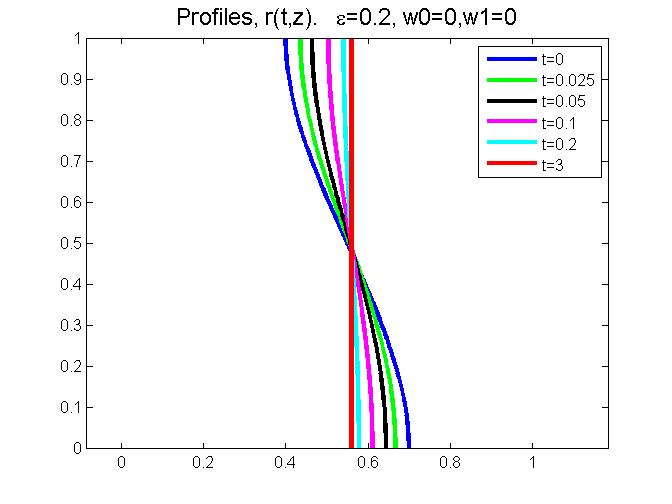
Refer to caption Refer to caption
(a) (b)
Refer to caption Refer to caption
(c) (d)
Figure 1: Example 5.1. Snapshots of surface profiles, values of energy functional, and volumes. ฯต=0.2italic-ฯต0.2\epsilon=0.2, rโ€‹(0,0)=0.7๐‘Ÿ000.7r(0,0)=0.7, rโ€‹(0,1)=0.4๐‘Ÿ010.4r(0,1)=0.4.
Example 5.2.

In this experiment, ฯต=0.2italic-ฯต0.2\epsilon=0.2, T=3๐‘‡3T=3, N=500๐‘500N=500, ฯ„=10โˆ’5๐œsuperscript105\tau=10^{-5}. The initial profile of r๐‘Ÿr is chosen to be the cubic Hermite interpolant that satisfies

rโ€‹(0,0)=0.4,rโ€‹(0,1)=0.2,rzโ€‹(0,0)=rzโ€‹(0,1)=0.formulae-sequence๐‘Ÿ000.4formulae-sequence๐‘Ÿ010.2subscript๐‘Ÿ๐‘ง00subscript๐‘Ÿ๐‘ง010\displaystyle r(0,0)=0.4,\quad r(0,1)=0.2,\quad r_{z}(0,0)=r_{z}(0,1)=0.

The results are shown in Figure ย 2. The initial volume is about 0.29800.29800.2980. Comparing with 0.98470.98470.9847, the volume in Example 5.1, this one is much smaller. However, the initial surface still evolves to a cylinder. Also, the errors in volumes (relative to the initial volume) are within 7ร—10โˆ’4%7percentsuperscript1047\times 10^{-4}\,\%.

Refer to caption Refer to caption
(a) (b)
Refer to caption Refer to caption
(c) (d)
Figure 2: Example 5.2. Snapshots of surface profiles, values of energy functional, and volumes. ฯต=0.2italic-ฯต0.2\epsilon=0.2, rโ€‹(0,0)=0.4๐‘Ÿ000.4r(0,0)=0.4, rโ€‹(0,1)=0.2๐‘Ÿ010.2r(0,1)=0.2.
Example 5.3.

In this experiment, ฯต=0.2italic-ฯต0.2\epsilon=0.2, T=3๐‘‡3T=3, N=500๐‘500N=500, ฯ„=10โˆ’5๐œsuperscript105\tau=10^{-5}. The initial profile of r๐‘Ÿr is chosen to be the cubic Hermite interpolant that satisfies

rโ€‹(0,0)=0.3,rโ€‹(0,1)=0.2,rzโ€‹(0,0)=rzโ€‹(0,1)=0.formulae-sequence๐‘Ÿ000.3formulae-sequence๐‘Ÿ010.2subscript๐‘Ÿ๐‘ง00subscript๐‘Ÿ๐‘ง010\displaystyle r(0,0)=0.3,\quad r(0,1)=0.2,\quad r_{z}(0,0)=r_{z}(0,1)=0.

The only difference between this example and Example 5.2 is the values of rโ€‹(0,0)๐‘Ÿ00r(0,0). The results are shown in Figure ย 3. However, this time it can be seen that singularity occurs.
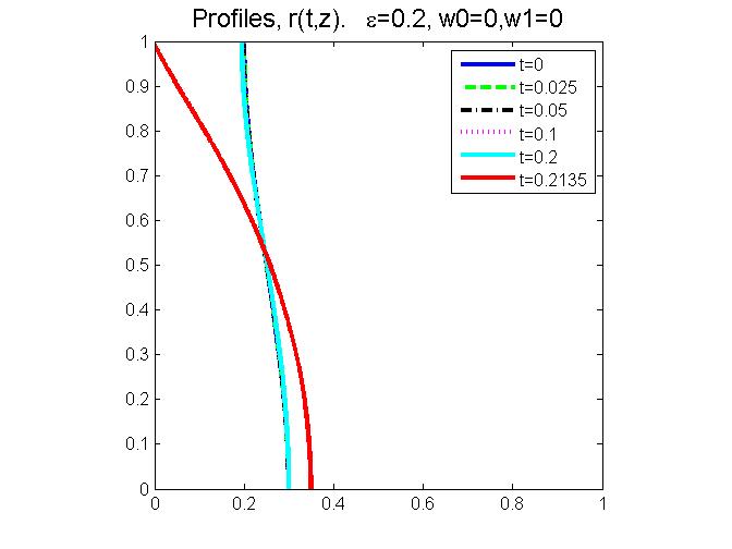
Refer to caption Refer to caption
(a) (b)
Refer to caption Refer to caption
(c) (d)
Figure 3: Example 5.3. Snapshots of surface profiles, values of energy functional, and volumes. ฯต=0.2italic-ฯต0.2\epsilon=0.2, rโ€‹(0,0)=0.3๐‘Ÿ000.3r(0,0)=0.3, rโ€‹(0,1)=0.2๐‘Ÿ010.2r(0,1)=0.2.
Example 5.4.

In this experiment, ฯต=0.2italic-ฯต0.2\epsilon=0.2, T=4๐‘‡4T=4, N=1000๐‘1000N=1000, ฯ„=10โˆ’6๐œsuperscript106\tau=10^{-6}. The initial profile of r๐‘Ÿr is chosen to be the cubic Hermite interpolant that satisfies
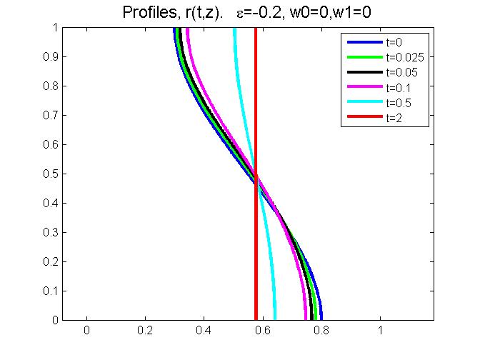
rโ€‹(0,0)=0.9,rโ€‹(0,1)=0.1,rzโ€‹(0,0)=rzโ€‹(0,1)=0.formulae-sequence๐‘Ÿ000.9formulae-sequence๐‘Ÿ010.1subscript๐‘Ÿ๐‘ง00subscript๐‘Ÿ๐‘ง010\displaystyle r(0,0)=0.9,\quad r(0,1)=0.1,\quad r_{z}(0,0)=r_{z}(0,1)=0.

The result is shown in Figure ย 4.

Refer to caption
Figure 4: Example 5.4. Snapshots of the 3D surfaces. ฯต=0.2italic-ฯต0.2\epsilon=0.2, rโ€‹(0,0)=0.9๐‘Ÿ000.9r(0,0)=0.9, rโ€‹(0,1)=0.1๐‘Ÿ010.1r(0,1)=0.1.
Example 5.5.

In this experiment, ฯต=0.4italic-ฯต0.4\epsilon=0.4, T=4๐‘‡4T=4, N=500๐‘500N=500, ฯ„=10โˆ’5๐œsuperscript105\tau=10^{-5}. The initial profile of r๐‘Ÿr is chosen to be the cubic Hermite interpolant that satisfies

rโ€‹(0,0)=0.3,rโ€‹(0,1)=0.2,rzโ€‹(0,0)=rzโ€‹(0,1)=0.formulae-sequence๐‘Ÿ000.3formulae-sequence๐‘Ÿ010.2subscript๐‘Ÿ๐‘ง00subscript๐‘Ÿ๐‘ง010\displaystyle r(0,0)=0.3,\quad r(0,1)=0.2,\quad r_{z}(0,0)=r_{z}(0,1)=0.

The results are shown in Figure ย 5.

Refer to caption
Figure 5: Example 5.5. Snapshots of the 3D surfaces. ฯต=0.4italic-ฯต0.4\epsilon=0.4, rโ€‹(0,0)=0.3๐‘Ÿ000.3r(0,0)=0.3, rโ€‹(0,1)=0.2๐‘Ÿ010.2r(0,1)=0.2.

Through these examples 5.2 to 5.5, we see that for small volume fractions, namely, when inequality (9) is not satisfied, the stability of cylinders is lost and singularity may develop, and therefore the flow may not exit for all time.

We present two more examples: In Example 5.6, ฯต<0italic-ฯต0\epsilon<0, in Example 5.7, a different initial profile is used. The results are shown in Figure ย 6 and Figure 7, respectively.

Example 5.6.

In this experiment, ฯต=โˆ’0.2italic-ฯต0.2\epsilon=-0.2, T=2๐‘‡2T=2, N=500๐‘500N=500, ฯ„=10โˆ’4๐œsuperscript104\tau=10^{-4}. The initial profile of r๐‘Ÿr is chosen to be the cubic Hermite interpolant that satisfies

rโ€‹(0,0)=0.8,rโ€‹(0,1)=0.3,rzโ€‹(0,0)=rzโ€‹(0,1)=0.formulae-sequence๐‘Ÿ000.8formulae-sequence๐‘Ÿ010.3subscript๐‘Ÿ๐‘ง00subscript๐‘Ÿ๐‘ง010\displaystyle r(0,0)=0.8,\quad r(0,1)=0.3,\quad r_{z}(0,0)=r_{z}(0,1)=0.
Refer to caption Refer to caption
(a) (b)
Refer to caption Refer to caption
(c) (d)
Figure 6: Example 5.6. Snapshots of surface profiles, values of energy functional, and volumes. ฯต=โˆ’0.2italic-ฯต0.2\epsilon=-0.2, rโ€‹(0,0)=0.8๐‘Ÿ000.8r(0,0)=0.8, rโ€‹(0,1)=0.3๐‘Ÿ010.3r(0,1)=0.3.
Example 5.7.

In this experiment, ฯต=0.2italic-ฯต0.2\epsilon=0.2, the initial profile is given by

rโ€‹(0,z)=1+14โ€‹cosโก(8โ€‹ฯ€โ€‹z).๐‘Ÿ0๐‘ง1148๐œ‹๐‘ง\displaystyle r(0,z)=1+\dfrac{1}{4}\cos(8\pi z).
Refer to caption Refer to caption
(a) (b)
Refer to caption Refer to caption
(c) (d)
Figure 7: Snapshots of surface profiles, values of energy functional, and volumes. ฯต=0.2italic-ฯต0.2\epsilon=0.2, rโ€‹(0,z)=1+cosโก(8โ€‹ฯ€โ€‹z)/4๐‘Ÿ0๐‘ง18๐œ‹๐‘ง4r(0,z)=1+\cos(8\pi z)/4.

References

  • [1] Andrews, Ben Volume-preserving anisotropic mean curvature flow. Indiana Univ. Math. J. 50 (2001), no. 2, 783โ€“827.
  • [2] Arroyo, Josu, Koiso, Miyuki and Palmer, Bennett; Stability of non liquid bridges, Preprint 2009.
  • [3] Athanassenas, Maria Volume-preserving mean curvature flow of rotationally symmetric surfaces. Comment. Math. Helv. 72 (1997), no. 1, 52โ€“66.
  • [4] Athanassenas, Maria Behaviour of singularities of the rotationally symmetric, volume-preserving mean curvature flow. Calc. Var. Partial Differential Equations 17 (2003), no. 1, 1โ€“16.
  • [5] Cabezas-Rivas, E. and Miquel, V; Volume preserving mean curvature flow of revolution hypersurfaces between two equidistants.
  • [6] K. ย Deckelnick, G. ย Dziuk, and C. M. ย Elliott, Computation of geometric partial differential equations and mean curvature flow, Acta. Numer. (2005), pp. ย  1โ€“94
  • [7] Ecker, Klaus Regularity theory for mean curvature flow. Progress in Nonlinear Differential Equations and their Applications, 57. Birkhรคuser Boston, Inc., Boston, MA, 2004.
  • [8] Giga, Yoshikazu Surface evolution equations. A level set approach. Monographs in Mathematics, 99. Birkhรคuser Verlag, Basel, 2006.
  • [9] Huisken, Gerhard The volume preserving mean curvature flow. J. Reine Angew. Math. 382 (1987).
  • [10] Koiso, Miyuki; Palmer, Bennett Geometry and stability of surfaces with constant anisotropic mean curvature. Indiana Univ. Math. J. 54 (2005), no. 6, 1817โ€“1852.
  • [11] Koiso, Miyuki; Palmer, Bennett Stability of anisotropic capillary surfaces between two parallel planes. Calc. Var. Partial Differential Equations 25 (2006), no. 3, 275โ€“298.
  • [12] Lunardi, Allesandra, Analytic Semigroups and Optimal Regularity in Parabolic Problems , Birkhรคuser Basel; 1 edition (May 12, 2003)
  • [13] McCoy, James A. Mixed volume preserving curvature flows. Calc. Var. Partial Differential Equations 24 (2005), no. 2, 131โ€“154.
  • [14] Taylor, Jean, Some mathematical challenges in materials science, Bulletin of The American Mathematical Society , vol. 40, no. 01, pp. 69-88, 2002
  • [15] Protter, M. H., Weinberger, H. F., Maximum Principles in Differential Equations. New York-Berlin-Heidelberg-Tokyo, Springer-Verlag 1984.


Bennett PALMER
Department of Mathematics

Idaho State University

Pocatello, ID 83209

U.S.A.

E-mail: palmbenn@isu.edu

Wenxiang ZHU

Department of Mathematics

Idaho State University

Pocatello, ID 83209

U.S.A.

E-mail: zhuwenx@isu.edu