Dynamics in the magnetic/dual magnetic monopole

Abstract

Inspired by the geometrical methods allowing the introduction of mechanical systems confined in the plane and endowed with exotic galilean symmetry, we resort to the Lagrange-Souriau 2-form formalism, in order to look for a wide class of 3D systems, involving not commuting and/or not canonical variables, but possessing geometric as well gauge symmetries in position and momenta space too. As a paradigmatic example, a charged particle simultaneously interacting with a magnetic monopole and a dual monopole in momenta space is considered. The main features of the motions, conservation laws and the analogies with the planar case are discussed. Possible physical realizations of the model are proposed.

1 Introduction

Originated by Lagrange and continued by Cartan [1], the geometrical formulation of the calculus of variations consists in mapping the Lagrangian function $L({\vec{x}},{\vec{p}},t):TQ\times\mathbb{R}\rightarrow\mathbb{R}$ into the so-called Cartan 1-form $\lambda$ over the evolution space $TQ\times\mathbb{R}$ and minimizing the corresponding action integral

$$\int_{\gamma}L(\gamma(t),\dot{\gamma}\left(t\right),t)dt=\int_{\widetilde{\gamma}}\lambda\quad\textrm{with}\quad\lambda=\frac{{\partial}L}{{\partial}p_{i}}dx^{i}+\left(L-\frac{{\partial}L}{{\partial}p_{i}}p_{i}\right)dt,$$ (1.1)

where $\widetilde{\gamma}=(\gamma(t),\dot{\gamma}\left(t\right),t)$ is the lifted world-line in the evolution space $TQ\times\mathbb{R}$ [2]. The exterior derivative of the Cartan form provides us with the closed Lagrange-Souriau 2-form $\sigma=d\lambda$. The associated Euler-Lagrange equations can be expressed by looking for the kernel of the 2-form $\sigma(\delta{\widetilde{\gamma}},\delta{\vec{y}})=0$, for any arbitrary movement $\delta{\vec{y}}$ in the evolution space. If the kernel is one-dimensional, i.e. the rank of $\sigma$ is $2d={\rm{dim}}\left(TQ\right)$, the variational problem is called regular, otherwise it is said singular and it is required to resort to the symplectic reduction techniques in order to describe the evolution space foliation in terms of ODE’s only [1, 2, 3, 4, 5].

Conversely, again following Souriau [2], a generalized mechanical system is defined by postulating the existence of a closed 2-form $\sigma$ on the evolution space , possessing constant rank $2d$. Then, its kernel defines an integrable foliation with $2d$-dimensional leaves, which can be viewed as generalized solutions of the variational problem. Moreover, by the Poincaré lemma, $d\sigma=0$ implies the existence of a Cartan $1$-form $\lambda$ only locally. In a local chart $\left({\cal U}\subseteq TQ\times\mathbb{R},\xi^{1},\ldots,\xi^{2d+1}\right)$ one can rewrite $\lambda$ as as $\lambda=a_{\alpha}d\xi^{\alpha}$ and plainly define a local first-order Lagrangian function as

$${\cal L}=a_{\alpha}\dot{\xi}^{\alpha}\quad\;\textrm{such that}\quad\;\int_{\widetilde{\gamma}\subset{\cal U}}\,\lambda=\int_{\gamma\subset{\pi\,\cal U}}{\cal L}dt.$$ (1.2)

Thus, for those models we do not have a usual Lagrange function like in (1.1) defined on the tangent bundle. Put in another way, the positions coordinates do not satisfy a second-order Newton equation. Moreover, Lagrangians of the type ${\cal L}$ in different intersecting charts ${\cal U}$ , ${\cal U}^{\prime}$ are related by patching procedures involving suitable transformations. The general question of the existence of Lagrangian has been discussed in [6]. Moreover, if the Lagrange-Souriau 2-form $\sigma$ can be split into a symplectic and a Hamiltonian part [2] $\sigma=\omega-dH\wedge dt,$ where $\omega$ is a closed and regular 2-form on the phase space $TQ$ and $H$ is a Hamiltonian function on $TQ\times\mathbb{R}$, than the equations of motion read $\omega\big{(}\dot{\widetilde{\gamma}}\big{)}=d\,H$. Because of the regularity of $\omega$, one introduces the co-symplectic matrix $(\omega^{\alpha\beta})$ ( i.e. $\omega^{\alpha\beta}\omega_{\beta\gamma}=\delta^{\alpha}_{\gamma}$), in such a way that the Poisson brackets are defined by $\{f,g\}=\omega^{\alpha\beta}{\partial}_{\alpha}f{\partial}_{\beta}g$ and the (Hamilton) equations of motion become $\dot{\xi}_{i}=\{\xi_{i},H\}$. In the case of singularity of $\omega$, again symplectic reductions have to be worked out.

On the other hand, in Souriau’s framework, one can state the so called inverse problem of the calculus of variations for a given set of equations of motion, describing a one-particle system in presence of a position-dependent force field ${\vec{E}}$ only. The set of equations can be rewritten as the set of 1-forms on $TQ\times\mathbb{R}$

$$\alpha_{1}=d{\vec{r}}-{\vec{v}}\;dt,\qquad\alpha_{2}=\;md{\vec{v}}-{\vec{E}}\;dt,$$ (1.3)

the kernels of both of them provide the intersections of a set of hyperplanes in the evolution space. Such an intersection is described also by the kernel of the 2-form obtained by the exterior product $\alpha_{1}\wedge\alpha_{2}\left(\delta y,\delta y^{\prime}\right)=\sigma\left(\delta y,\delta y^{\prime}\right)=0\;$. In presence of an electromagnetic field ${\vec{E}}\left({\vec{r}},t\right),{\vec{B}}\left({\vec{r}},t\right)$ acting on a charge $e$, Souriau [2] generalized the previous simplest 2-form to

$$\sigma = \left(md{\vec{v}}-e{\vec{E}}dt\right)\wedge\left(d{\vec{r}}-{\vec{v}}dt\right)+e{\vec{B}}\cdot d{\vec{r}}\times d{\vec{r}},$$ (1.4)

where we have defined $\left(d{\vec{r}}\times d{\vec{r}}\right)_{k}=\frac{1}{2}\epsilon_{kij}dx_{i}\wedge dx_{j}$. Then, the usual equations of motion of a charged particle in the electromagnetic field are seen to arise as the kernel of $\sigma$, together with the closure condition $d\sigma=0$, leading to the the homogeneous Maxwell equations for the ${\vec{E}}$ and ${\vec{B}}$ fields. These formulas can be readily generalized to the multi-particles case.

Now, in the same spirit we would like to write down a Lagrangian 2-form for a particle of mass $m$, which is subjected both to the electromagnetic field $\left\{{\vec{E}}\left({\vec{r}},t\right),\;{\vec{B}}\left({\vec{r}},t\right)\right\}$ and to a peculiar ”environment”, in the sense that the relation between ${\vec{p}}$ and ${\vec{v}}$ is more general than how much it was described before.

The simplest example of such a situation is the exotic mechanical model in the 2-dimensional plane proposed by [7]. It is defined by a generalization of the (1.4) form, precisely we introduce

$$\sigma=dp_{i}\wedge dx_{i}+\theta\,dp_{1}\wedge{}dp_{2}+eB\,dx_{1}\wedge dx_{2}-d\left(\frac{\vec{p}{\,}^{2}}{2m}+eV\right)\wedge dt,$$ (1.5)

where ${\vec{p}}=m\,{\vec{v}}$, $B\left({\vec{r}}\right)$ is the magnetic field, perpendicular to the plane, $V\left({\vec{r}}\right)$ the electric potential (both of them assumed to be time-independent for simplicity) and $\theta$ is a constant, called the non-commutative parameter, for reasons clarified below. The resulting equations of motion read [7]

$$m^{*}\dot{x}_{i}=p_{i}-\displaystyle em\theta\,\epsilon_{ij}E_{j},\qquad\displaystyle\dot{p}_{i}=e\,E_{i}+e\,B\,\epsilon_{ij}\dot{x}_{j},$$ (1.6)

where we have introduced the effective mass $m^{*}=m\;(1-e\;\theta\;B).$ The physical novelties are: i) the anomalous velocity term $-\displaystyle em\theta\,\epsilon_{ij}E_{j}$, so that $\dot{{\vec{r}}}\nparallel{\vec{p}}$, ii) the derivative of the kinetic momentum ${\vec{p}}$ is still determined by the Lorentz force, iii) the interplay between $\theta$ and $B$ field in $m^{*}$. The 2-form (1.5) can obtained by exterior derivation of the Cartan 1-form

$$\lambda=({p_{i}}-{A_{i}}\,)d{x_{i}}-\left(\frac{\vec{p}{\,}^{2}}{2m}+e\,V\right)\,dt+\frac{\theta}{2}\,\epsilon_{ij}\,{p_{i}}\,d{p_{j}}$$ (1.7)

defining the action functional as in (1.2) and involving the vector potential components $A_{i}$. Notice that $\lambda$ is gauge dependent, in contrast with the 2-form $\sigma$, in which only observable (i.e. gauge invariant) quantities appear. Furthermore, for $m^{*}\neq 0$ (1.5) can be split in hamiltonian form, leading to the Poisson brackets

$$\begin{array}[]{lll}\{x_{1},x_{2}\}=\displaystyle\frac{m}{m^{*}}\,\theta,\quad\{x_{i},p_{j}\}=\displaystyle\frac{m}{m^{*}}\,\delta_{ij},\quad\{p_{1},p_{2}\}=\displaystyle\frac{m}{m^{*}}\,eB,\end{array}$$ (1.8)

which satisfy the Jacobi identity for any $B$ field. When the effective mass vanishes, i.e. when the magnetic field takes the critical value $B_{crit}=\frac{1}{e\theta}$, the system becomes singular. Then, the symplectic reduction procedure leads to a two-dimensional system characterized by the remarkable Poisson structure $\{x_{1},x_{2}\}=\theta$, reminiscent of the “Chern-Simons mechanics” [8]. Thus, the symplectic plane plays, simultaneously, the role of both configuration and phase space. The only motions are those following the Hall law $p_{i}=\varepsilon_{ij}\frac{E_{j}}{B_{crit}}$. Moreover, in the quantization of the reduced system, not only the position operators no longer commute, but the quantized equation of motions yields the Laughlin wave functions [9], which are the ground states in the Fractional Quantum Hall Effect (FQHE). Thus, one can claim that the classical counterpart of the anyons are in fact the exotic particles in the system (1.6). In the review article [10] several examples of 2-dimensional models, which generalize the form (1.5) and the equations (1.6) have been discussed. Here let us recall that the Poisson structure (1.8) can be obtained by applying the Lie-algebraic Kirillov-Kostant-Souriau method for constructing dynamical systems, possessing the (2+1)- Galilei group endowed with a 2-fold central extension [11, 12]. The two cohomological parameters are the usual mass $m$ and an “exotic” parameter $\theta$, describing the non-commutativity of Galilean boost generators

$$\left\{K_{1},K_{2}\right\}=-\theta m^{2}.$$ (1.9)

In the context of the condensed matter physics, $\theta$ can be identified with a constant Berry curvature, generated by the lattice structure, acting on electron wave-packets [14]. On the other hand, it can be also viewed as a “non-relativistic shadow of the spin” for a relativistic particle, by performing the so-called “Jackiw-Nair” contraction [15]. The main result is that the last term in (1.7) can be replaced with a suitable ${\vec{p}}$-dependent $A_{j}\left({\vec{r}},{\vec{p}}\right)\,dp_{j}$ 1-form, which provides a convenient curvature in the momentum space, like the parameter $\theta$ does in the above example.

2 The general model in (3+1)-dim

Now, let us look for a further generalizations [13] - [16] of the 2-form (1.4) with momentum dependent fields. Straightforward algebraic considerations lead to define the manifestly anti-symmetric covariant 2-tensor on the evolution space

$$\sigma = \left[\left(1-\mu_{i}\right)dp_{i}-e\;E_{i}\;dt\right]\wedge\left(dr_{i}-g_{i}\;dt\right)+{\scriptstyle{\frac{1}{2}}}\;e\;B_{k}\;\epsilon_{kij}\;dr_{i}\wedge dr_{j}+$$ (2.10)

$${\scriptstyle{\frac{1}{2}}}\;\kappa_{k}\;\epsilon_{kij}\;dp_{i}\wedge dp_{j}+q_{k}\;\epsilon_{kij}\;dr_{i}\wedge dp_{j},$$

where we have put into evidence the usual Lorentz force contributions as in (1.5), while the 3-vectors ${\vec{g}}$, $\vec{\kappa}$, the diagonal $3\times 3$-matrix $Q=\textrm{diag}\left(\mu_{i}\right)$ and the anti-symmetric one $\left(Q_{A}\right)_{ij}=\epsilon_{ijk}\;q_{k}$ depend on all independent variables and have to be determined in such a way that $d\,\sigma=0$ ( the “Maxwell Principle” by [2]) and to have constant rank. Similarly to the effective mass concept in solid state physics, by the expression $1-\mu_{i}$ we would like to distinguish between the bare mass, normalized to 1, and a possible ”local” contribution. With respect to the expression (1.3)-(1.5), we introduced the 1-form $dr_{i}-g_{i}\;dt$, which defines a general relation between the conjugate momentum and the velocity.

The equations of motion can be written as the kernel of $\sigma\left(\delta y,\cdot\right)=0$ of the Lagrange-Souriau form, for any tangent vector $\delta y=\left(\delta{\vec{r}},\delta{\vec{p}},\delta t\right)$. Specifically one obtains the equations

$$e\;\delta{\vec{r}}\cdot{\vec{E}}-\left(1-Q\right)\delta{\vec{p}}\cdot{{\vec{g}}} = 0,$$ (2.11)

$$\left(1-Q-Q_{A}\right)\delta{\vec{p}} = e\left({\vec{E}}\;\delta t+\;\delta{\vec{r}}\times{\vec{B}}\right),$$ (2.12)

$$\left(1-Q\right)\;\left(\delta{\vec{r}}-{\vec{g}}\;\delta t\right) = {-\delta{\vec{r}}\times\vec{q}}\;-\delta{\vec{p}}\times{\vec{\kappa}}\;.$$ (2.13)

Equation (2.12) can be solved for $\delta{\vec{p}}$, if the matrix $M={\mathbf{1}}-Q-Q_{A}$ is invertible. Under such an hypothesis together with ${\rm det}\left(1-Q\right)\neq 0$, one replaces $\delta{\vec{p}}$ in the equation (2.13), finding an equation for the position tangent vector $\delta{\vec{r}}$, i.e.

$$M^{*}\;\delta{\vec{r}}=\left(\left(1-Q\right){\vec{g}}+e\;{\cal K}M^{-1}\cdot{\vec{E}}\right)\delta t,$$ (2.14)

where the effective mass matrix is given by

$$M^{\star}=M+\left(2Q_{A}-e\;{\kappa}M^{-1}{\cal B}\right)\;,\quad{\kappa}_{ij}=\epsilon_{ijk}\kappa_{k}\;,\;{\cal B}_{ij}=\epsilon_{ijk}B_{k}.$$ (2.15)

Both $M^{*}$ and the eq. (2.14) generalize of the expressions obtained in [7] leading to (1.6). Singularities in the motion can arise from the vanishing of ${\rm det}\left(M\right)$, ${\rm det}\left(1-Q\right)$ and ${\rm det}\left(M^{*}\right)$. However, if it is not the case, one can solve (2.14) w.r.t $\delta{\vec{r}}$ and show that

1. equation (2.11) is identically satisfied independently from the specific choice for the vector $\vec{g}$,

2. the equation (2.12) becomes

   $$M^{*}\delta{\vec{p}}=\frac{e}{{\rm det}\left(M\right)}\left(R\;{\vec{E}}-{\vec{g}}^{\;T}N{{\vec{B}}}\right)\delta t,$$ (2.16)

   where matrices $R$ and $N$ have an involved dependency on $m$, ${\vec{B}}$, $\vec{\kappa}$, $Q$ and $Q_{A}$ to be spelled here.

Since the pfaffian equations (2.14)-(2.16) can be proved to be integrable, they are equivalent to the simultaneous first order differential equations particle position ${\vec{r}}$ and for the variable ${\vec{p}}$, which in the hamiltonian formulation (see Sec. 3) will play the role of particle momentum, assuming ${\vec{g}}={\vec{p}}$. Moreover, under such a hypothesis, the two equations of motion simplify to the system (1.6) when $Q$ and $Q_{A}$ are set to 0.

Now, accepting as a law of mechanics [2] the closure condition $d\sigma=0$ for (2.10), we impose the vanishing of the coefficients of the independent $3$-forms. It is quite natural to assume the limitations: ${\partial}_{p_{i}}E_{j}={\partial}_{p_{i}}B_{j}=0$ . Thus we are lead to the equations

$${\partial}_{r_{j}}B_{j}=0, \varepsilon_{kij}{\partial}_{r_{i}}E_{j}=-{\partial}_{t}B_{k},$$ (2.17)

$${\partial}_{p_{j}}\kappa_{j}=0, \varepsilon_{kij}{\partial}_{p_{i}}\left[\left(1-\mu_{j}\right)g_{j}\right]={\partial}_{t}\kappa_{k},$$ (2.18)

$${\partial}_{t}\mu_{i}={\partial}_{r_{i}}\left[\left(1-\mu_{i}\right)g_{i}\right], {\scriptstyle{\frac{1}{2}}}\varepsilon_{kij}\;{\partial}_{r_{i}}\,\left[\left(1-\mu_{j}\right)g_{j}\right]={\partial}_{t}q_{k},$$ (2.19)

$${\partial}_{r_{i}}\;\mu_{j}=\varepsilon_{ijk}{\partial}_{r_{j}}q_{k}, {\partial}_{r_{i}}\kappa_{j}=\varepsilon_{ijk}{\partial}_{p_{k}}\;\mu_{i}+{\partial}_{p_{i}}\;q_{j}-\delta_{ij}{\partial}_{p_{k}}\;q_{k},$$ (2.20)

$${\partial}_{r_{j}}\left[\left(1-\mu_{i}\right)g_{i}\right]+ {\partial}_{r_{i}}\left[\left(1-\mu_{j}\right)g_{j}\right]=0,\qquad i\neq j=1,2,3.\qquad$$ (2.21)

One can observe that the homogeneous Maxwell equations (2.17) are the only restrictions on the electromagnetic fields $\left({\vec{E}},{\vec{B}}\right)$. Equations (2.18) are the analogs of the previous relations in the momentum space for the vector-field $\vec{\kappa}$. For such a reason, sometimes $\vec{\kappa}$ is called dual magnetic field. As we will see in the Hamiltonian formalism, its existence implies the non-commutativity of the spatial coordinates.

If $\vec{\kappa}$ is non trivial in time, then a change in the velocity dependence is induced for the mass flow $\left(\mathbf{1}-Q\right){\vec{g}}$, as prescribed by the second equation in (2.18). In its turn, equations (2.19) say how the particle mass may change in time. This seems to be a quite unusual situation, but we cannot discard it at the moment. On the other hand, the first set of three equations in (2.19) has the form of independent continuity equations, leading to the global conservation law for the total mass, i.e. ${\partial}_{t}\left(\sum_{i}\mu_{i}\right)+{\partial}_{r_{i}}\left[\left(1-\mu_{i}\right)g_{i}\right]=0$, which however holds separately in different directions. Also the skew-symmetric contributions to the mass matrix $M$ may change on time, but they generate modification of the mass flux in space, accordingly to the second set of equations in (2.19).

The equations in (2.20) are more difficult to interpret: they provide consistency relations for both the space and the momentum dependency among the mass matrix elements and the dual magnetic field. Putting such expressions into the equation of motion in the form (2.12)-(2.13), in a pure axiomatic way one re-obtains the equations found in the context of the semiclassical motion of electronic wave-packets in [14].

For a particle with constant mass, i.e. for $\mu_{i}\equiv 0$ and momentum ${p_{i}}=g_{i}$, one easily concludes that $\vec{\kappa}$ and ${\vec{q}}$ have to be constants. A further analysis of the closure relations (2.19)-(2.20) leads to the expression $\kappa_{i}=\sum_{j\neq i}\left(x_{j}{\partial}_{p_{j}}q_{i}-x_{i}{\partial}_{p_{j}}q_{j}\right)+\chi_{i}$, where the $q_{i}$’s and $\chi_{i}$ ’s depend only on ${\vec{p}}$ and moreover the divergenceless condition ${\partial}_{p_{j}}\chi_{j}=0$ has to be satisfied.

Limiting ourselves to two spacial dimensions and setting $\kappa_{3}=-\theta$, we reobtain the model (1.6) above. More generally a momentum-dependent non-commutativity field $\kappa_{3}=\kappa({\vec{p}})$ was considered in the Snyder space [17], with $\kappa=-\frac{\theta}{1+\theta p^{2}}\varepsilon_{ij}p_{i}r_{j}$ (and $\mu_{i}\equiv 0$ ), or for the relativistic spinning particle in the plane, with $\kappa^{\alpha\beta}=\frac{s}{2}\frac{p_{\alpha}\epsilon^{\alpha\beta\gamma}}{(p^{2})^{3/2}}$ [18, 19]. In 3 dimensions it is provided the remarkable example of the monopole field in momentum space ${\vec{\kappa}}=\theta\frac{{\vec{p}}}{|{\vec{p}}|^{3}}$, which admits the spherical symmetry and the canonical relations $\{r_{i},p_{j}\}=\delta_{ij}$, describing the Poisson structure of the phase space of a 0-mass relativistic particle with non-vanishing helicity (photon) [2], [20]. Its expression appears to be consistent with the experimental data reported for the Anomalous Hall Effect [21] and in Spin Hall Effect [22] and are theoretically discussed in [23] and [24].

Finally, in the singular submanifold of the phase space defined by $M^{*}=0$, we need to look at the proper restrictions on vector-fields ${\delta{\vec{p}}}$ and ${\delta{\vec{r}}}$, in order to avoid motions with infinite velocities. Those restrictions generalize the Hall law discussed in the previous Section.

3 Hamiltonian Structure

The 2-form $\sigma$ in (2.10) can be obtained as the exterior derivative of the Cartan 1-form,

$$\lambda=\left({\vec{p}}-\overrightarrow{{\cal A}}\right)\cdot d{\vec{r}}+{\vec{\cal R}}\,\cdot d{\vec{p}}-{\cal T}\,dt.$$ (3.22)

In this formula the field $\overrightarrow{{\cal A}}\left({\vec{r}},t\right)$ is the usual electromagnetic potential, such that ${\vec{B}}=\nabla_{{\vec{r}}}\times\overrightarrow{{\cal A}}$, for which we have postulated to be momentum-independent. The field $\overrightarrow{{\cal A}}$ admits the usual gauge arbitrariness. On the other hand, the electric field is given by ${\vec{E}}=-\nabla_{{\vec{r}}}{\cal T}-{\partial}_{t}\overrightarrow{{\cal A}}$, where we assume that ${\cal T}\left({\vec{r}},{\vec{p}},t\right)={\cal E}\left({\vec{p}},t\right)+\varphi\left({\vec{r}},t\right)$, in order to be stuck to the previous assumption about the dependency of ${\vec{E}}$. Furthermore, the field ${\vec{\cal R}}\left({\vec{r}},{\vec{p}},t\right)$ defines the dual magnetic field $\vec{\kappa}=\nabla_{{\vec{p}}}\times{\vec{\cal R}}$, the mass flow $\left(\mathbf{1}-Q\right){\vec{g}}=-\nabla_{{\vec{p}}}{\cal T}-{\partial}_{t}{\vec{\cal R}}$, the mass components $\mu_{i}={\partial}_{r_{i}}{\cal R}_{i}$ and $q_{k}={\partial}_{r_{i}}{\cal R}_{j}=-{\partial}_{r_{j}}{\cal R}_{i}$ ($k,i,j$ cyclic). Also ${\vec{\cal R}}$ admits the gauge arbitrariness both in position and momentum variables. Thus the the entire evolution space is decomposed in patches, on which the Cartan 1-form (3.22) defines local connections, related by gauge transformations satisfying the Maxwell-type equations (2.17)-(2.21). In particular, expressed in terms of the gauge field ${\cal R}$ , the closure relations in (2.19) and (2.20) become

$${\partial}_{r_{i}}{\partial}_{r_{j}}{\cal R}_{k}=0\quad\textrm{( $i,j,k$ cyclic)},\qquad{\partial}_{r_{i}}^{2}{\cal R}_{j}=-{\partial}_{r_{i}}{\partial}_{r_{j}}{\cal R}_{i}\;\;\left(i\neq j\right),$$ (3.23)

$${\partial}_{t}\left({\partial}_{p_{i}}{\cal R}_{j}+2{\partial}_{p_{j}}{\cal R}_{i}\right)=0\qquad i\neq j,$$ (3.24)

with no summation over repeated indices in the first two equations. Due to the special form we assumed on the force and magnetic fields, the above restrictions on $\vec{\cal R}$ limit its space-time dependency, leaving however the gauge freedom with respect the momentum variables. As it has been elsewhere remarked [10], it is possible to perform a change of variables leading to commutative position variables by a point transformation of the form $r_{i}\to r^{\prime}_{i}=r_{i}-{\cal R}_{i}({{\vec{r}}},{{\vec{p}}})$. However, the vector field $\vec{\cal R}$ is defined up to a gauge transformation generated by an arbitrary function on $\left({\vec{r}},{\vec{p}}\right)$. Thus, the meaning of the notion of position is unclear in such a context.

If ${\partial}_{t}\vec{{\cal A}}={\partial}_{t}\vec{{\cal R}}\equiv 0$, it is possible to split (2.10) in the hamiltonian form $\sigma=\omega-d{\cal T}\wedge dt$, by introducing on $TQ=\left\{\xi=\left({\vec{r}},{\vec{p}}\right)\right\}$ the symplectic 2-form

$$\omega=\left(\delta_{i,j}+\chi_{ij}\,\right)dp_{\;i}\wedge dr_{\;j}+\frac{1}{2}\left[b_{ij}\,dr_{\;i}\wedge dr_{\;j}+\kappa_{ij}\,dp_{\;i}\wedge dp_{\;j}\right],$$ (3.25)

where

$$\chi_{ij}=\left\{\begin{array}[]{ll}-{\partial}_{r_{j}}{\cal R}_{i},&i\leq j\\ {\partial}_{r_{i}}{\cal R}_{j},&i>j\\ \end{array}\right.\quad b_{ij}=-\varepsilon_{ijk}B_{k},\quad\kappa_{ij}=\varepsilon_{ijk}\kappa_{k}.$$ (3.28)

and the equations of motion take the Hamilton form. Moreover, the closure of $\omega$ is assured by that one of $\sigma$, i.e. by the equations (2.17) - (2.21), and their consequences (3.23). Then, accordingly to the general expression (1), the space $TQ$ is endowed with the Poisson structure expressed by the co-symplectic matrix

$$\omega^{\alpha,\beta}=\Big{(}1-\frac{1}{2}{\rm Tr}\left(\chi^{2}+b\left({\bf 1}+2\,\chi\right)\kappa\right)\Big{)}^{-1}$$ (3.29)

$$\left\{\left({\begin{array}[]{cc}\kappa+\left[\chi,\kappa\right]&0\\ 0&-b+\left[\chi,b\right]\\ \end{array}}\right)+\left[1-\frac{1}{2}{\rm Tr}\left(\chi^{2}+b\,\kappa\right)\right]\left({\begin{array}[]{cc}0&1\\ -1&0\\ \end{array}}\right)+\right.$$ (3.34)

$$\left.\left({\begin{array}[]{cc}0&\left(\chi^{2}+b\,\kappa\right)^{T}\\ -\left(\chi^{2}+b\,\kappa\right)&0\\ \end{array}}\right)\right\},$$ (3.37)

non degenerate for $\sqrt{\det\left(\omega_{\alpha\beta}\right)}=1-\frac{1}{2}{\rm Tr}\left(\chi^{2}+b\left({\bf 1}+2\,\chi\right)\kappa\right)\neq 0.$ Such a factor generalizes the denominators present in the Poisson brackets (1.8) or (2.15). Moreover, it crucially appears in the expression of the invariant phase-space volume, ensuring the validity of the Liouville theorem. Finally, notice that the Poisson structure is determined only by gauge invariant quantities and brackets involving position coordinates $r_{i}$ are in general non-commutative. Several examples systems which can be written in the above formalism are given in [10], in the following we will discuss the double monopole model.

4 The double monopole

For a charge subjected only to a monopole in the momentum space, of strength $\theta$, and to a uniform electric field ${\vec{E}}$, the above procedure leads to equations of motion readily integrable. [24]. The main feature is that the particle suffers a shift $\Delta=\frac{2\theta}{p_{0}}$ in the direction ${\vec{E}}\times{\vec{p}}_{0}$, being ${\vec{p}}_{0}$ the initial linear kinetic momentum. This is an important result in controlling spin currents only by electric fields [21].

Now, it is natural to consider an electric charge simultaneously subject to a momentum space (or dual) monopole and to a magnetic monopole. From theoretical side, this restores the ”symmetry” lost in the model described in [20]. On the other hand one may figure out a concrete realization of such a model, on the base of the experimental evidence of isolated monopole excitations in the ice-spin compounds [25], or of the proposal [26] in a different context. To include also the effects of a dual monopole, one needs to find a suitable behavior of the Berry phase got by an electron wave-packet moving in the lattice, as described in [14]. For brevity, such a system will be called a double monopole. The symplectic structure can be ready derived from expressions (3.25) or (3.37) and it can be expressed by the co-symplectic form

$$\omega^{\alpha,\beta}=\frac{1}{M^{*}}\left(\begin{array}[]{cc}\theta|{\vec{r}}|^{3}\,\tilde{p}&-|{\vec{r}}|^{3}|{\vec{p}}|^{3}{\bf 1}-e\,\theta\left({\vec{p}}\otimes{\vec{r}}\right)^{T}\\ |{\vec{r}}|^{3}|{\vec{p}}|^{3}{\bf 1}+e\,\theta{\vec{p}}\otimes{\vec{r}}&e\,|{\vec{p}}|^{3}\,\tilde{r}\end{array}\right),$$ (4.38)

having introduced $e$ for the charge-magnetic monopole coupling constant, $\tilde{p}_{ij}=\varepsilon_{i\,j\,k}p_{k}$, $\tilde{r}_{ij}=\varepsilon_{i\,j\,k}r_{k}$ and the effective mass

$$M^{*}=|{\vec{r}}|^{3}|{\vec{p}}|^{3}-e\theta\;{\vec{r}}\cdot{\vec{p}}.$$ (4.39)

From (4.38) one gets $\sqrt{\det\left(\omega^{\alpha,\,\beta}\right)}=\frac{|{\vec{r}}|^{3}|{\vec{p}}|^{3}}{M^{*}}$. Then, the vanishing of the effective mass $M^{*}$ will provide an anholonomic constraint to the dynamics.

Assuming that no other field is present, a charged particle of unitary mass in a double monopole has the free Hamiltonian $H=\frac{|{\vec{p}}|^{2}}{2}$, so that the equations of motion are

$$M^{*}\dot{r}_{i} = \left(p_{i}-e\theta\frac{r_{i}}{|{\vec{p}}||{\vec{r}}|^{3}}\right)|{\vec{r}}|^{3}|{\vec{p}}|^{3},\;$$ (4.40)

$$M^{*}\dot{p}_{i} = e\varepsilon_{ijk}p_{j}r_{k}|{\vec{p}}|^{3}.$$ (4.41)

On the other hand, the expression

$$\vec{j}={\vec{r}}\times{\vec{p}}-\frac{\theta}{|{\vec{p}}|}{\vec{p}}-\frac{e}{|{\vec{r}}|}{\vec{r}}$$ (4.42)

is conserved during the motion. Moreover, its components satisfy the commutation relations $\left\{j_{i},j_{j}\right\}=\varepsilon_{i,\,j,\,k}j_{k}$, as well as to commute with the Hamiltonian with respect to the Poisson structure (4.38). Then $\vec{j}$ is identified with the total angular momentum, involving both the usual expression for such a quantity for a Dirac monopole and for a dual monopole, as in [23], [27]. The usual arguments about the Liouville integrability for a central system may be applied here, in order to make the double monopole system an integrable model. However, the breaking of the Jacobi identities ${\scriptstyle{\frac{1}{2}}}\varepsilon_{ijk}\left[p_{i},\left[p_{j},p_{k}\right]\right]=e\,\delta\left({\vec{r}}\right)$ and ${\scriptstyle{\frac{1}{2}}}\varepsilon_{ijk}\left[r_{i},\left[r_{j},r_{k}\right]\right]=\theta\,\delta\left({\vec{p}}\right)$ makes that conclusion questionable. On the other hand, the above breaking suggest that a quantum treatment of the problem provides a quantization both of the magnetic charge $e=N_{m}/2$ and of the dual one $\theta=N_{d}/2$ [23].

A remarkable fact is that the modulus of $\vec{j}$ takes a non vanishing minimum, since it results

$$|{\vec{j}}|^{2}=\left({\vec{r}}\times{\vec{p}}\right)^{2}+\left(|\theta|+|e|\right)^{2}-4|e\,\theta|\,\left\{\begin{array}[]{ll}\textrm{sign}\left(e\theta\right)=1,&\sin^{2}\\ \textrm{sign}\left(e\theta\right)=-1,&\cos^{2}\end{array}\right.\left(\frac{\widehat{{\vec{r}}\,{\vec{p}}}}{2}\right),$$ (4.43)

which is achieved in particular when ${\vec{p}}\,\|\,{\vec{r}}$. Certainly, it is not surprising that a 0-mechanical angular momentum electric charge - magnetic monopole system possesses a non vanishing total angular momentum [28], but here, a part from the presence of both coupling constants, the state is achieved dynamically along particular trajectories, intersecting in the phase space the 5-dimensional unbounded sub-manifold of the vanishing effective mass, say $\cal M$. They can exist, since the invariant manifold of constant total energy is compact only in the momentum subspace, but the constant angular momentum sub-manifold may do not intersect $\cal M$, since it depends both on the position and the linear momenta variables. Notice that the Poisson brackets $\left\{M^{*},H\right\}$ are not vanishing, but restricting them on $\cal M$ one obtains

$$\left\{M^{*},H\right\}|_{\cal M}=3|{\vec{p}}|^{2}\left(|{\vec{r}}|^{4}|{\vec{p}}|^{4}-e^{2}\theta^{2}\right){\vec{p}}\cdot{\vec{r}}.$$ (4.44)

This relation and $M^{*}$ itself vanish consistently with the parallelism condition

$$p_{i}=\textrm{sign}\left(e\theta\right)\sqrt{|e\theta|}\frac{r_{i}}{|{\vec{r}}|^{2}},$$ (4.45)

which is dictated by the equations of motion (4.40)-(4.41). Thus a particle trajectory which reaches the manifold $\cal M$ will remain confined on it. In this limit equation (4.41) is identically satisfied, while equation (4.40) becomes

$$\dot{r}_{i}=\textrm{sign}\left(e\theta\right)\sqrt{|e\theta|}\frac{r_{i}}{|{\vec{r}}|^{2}},$$ (4.46)

noticing that now the velocity and linear momentum are now proportional (actually equal, having set the mass unitary). Moreover total angular momentum takes the value $\vec{j}=-\textrm{sign}\left(e\right)\left(|\theta|+|e|\right)\frac{{\vec{r}}}{|{\vec{r}}|}$, which has minimal modulus. Then, for any initial data $\left\{{\vec{r}}_{0},\,{\vec{p}}_{0}\right\}$, such that $|{\vec{j}}_{0}|=|\theta|+|e|$, there exists a position directed as $\frac{{\vec{r}}_{cr}}{|{\vec{r}}_{cr}|}=-\textrm{sign}\left(e\right)\frac{{\vec{j}}_{0}}{|\theta|+|e|}$ along which the constraint (4.45) can be satisfied for the first time. Since in such a position, the Hamiltonian takes the value $H|_{\cal M}=\frac{|e\theta|}{2|{\vec{r}}_{cr}|^{2}}=E_{0}$, being $E_{0}$ its value at the initial point, one concludes that $|{\vec{r}}_{cr}|=\sqrt{\frac{|e\,\theta|}{2E_{0}}}$, or

$${\vec{r}}_{cr}=-\textrm{sign}\left(e\right)\frac{\sqrt{|e\theta|}}{|\theta|+|e|}\frac{\vec{j}_{0}}{\sqrt{2\,E_{0}}}.$$ (4.47)

Substitution into (4.46), one gets the velocity $\dot{{\vec{r}}}_{cr}=\sqrt{2E_{0}}\frac{{\vec{r}}_{cr}}{|{\vec{r}}_{cr}|}$ of the particle, which from now will follows a restricted dynamics.

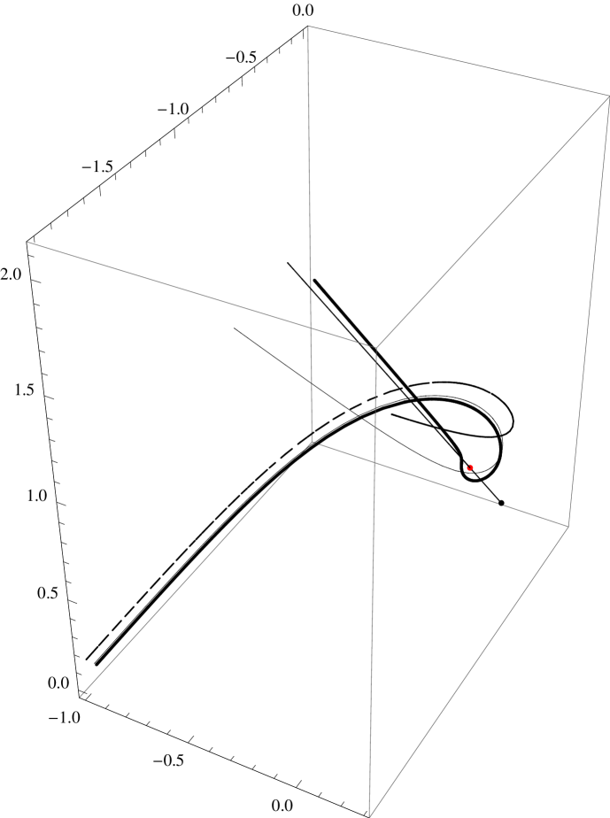
Figure 1: Detailed view of the scattering of three charges on a double monopole, showing the details of the trajectory for a particle which is close to be captured in the 0-effective mass sub-manifold ( thick curve), in comparison with two others of increasing angular momentum (thin continuous, then dashed curve). The straight line from the origin indicates the final trajectory of corresponding 0-effective mass particle and the red point the position ${\vec{r}}_{cr}$.

In fact, on the invariant critical sub-manifold $\cal M$ the symplectic 2-form $\omega$ reduces to

$$\omega|_{\cal M}={\scriptstyle{\frac{1}{2}}}\varepsilon_{ijk}\frac{e}{|{\vec{r}}|^{3}}\left(1+|\frac{\theta}{e}|\right)r_{k}dr_{i}\wedge dr_{j},$$ (4.48)

which is proportional by the $\frac{e}{|{\vec{r}}|^{3}}$ factor to the symplectic 2-form induced on $so\left(3\right)^{*}$ by the $SO\left(3\right)$ co-adjoint action. Resorting to the usual spherical foliation, with induced Poisson brackets $\left\{\vartheta,\varphi\right\}=-\left[|e|\left(|\frac{\theta}{e}|+1\right)|{\vec{r}}|^{2}\sin\varphi\right]^{-1}$ for the angular variables, one obtains trivial equations of motion $\dot{\vartheta}=\dot{\varphi}=0$, since the Hamiltonian is only radius dependent. Then, $\left(\vartheta,\varphi\right)$ will be fixed by $\frac{{\vec{r}}_{cr}}{|{\vec{r}}_{cr}|}$, while the radius will increase linearly accordingly to

$$|{\vec{r}}|=\sqrt{2E_{0}}\,t+|{\vec{r}}_{cr}|.$$ (4.49)

Thus, in the case of double monopole this result realizes the Hall motions described in Sec. 1, with a very similar mechanism based on the interplay of magnetic field and its dual counterpart in the momentum space.

5 Conclusions

In conclusion, a wide set of dynamical systems can be derived from the Lagrange-Souriau 2-form approach in 3-dimensions. Generalizations to higher number of degrees of freedom seems straightforward. We have shown the conditions to assure their Hamiltonian formulation. From which an analysis for their integrability properties can be pursued more plainly, by resorting to standard methods. However, one should check if the first order Lagrangian formalism can be used equally well, as suggested in [10] Sec. 4. In this perspective, it should be made a remark in connection with the procedure, sometime said of the minimal addition, of coupling the mechanical system to the the electromagnetic field adopted in (2.10). It is quite different from the usual minimal coupling procedure, which yields a very different Poisson structure. In the context of the 2-dimensional systems the two formulations were proved to be equivalent under a classical Seiberg-Witten transformation of electromagnetic fields [10], but no results are yet available in 3D and this hole should be filled in future works. In the present article we have discussed in detail the double monopole system, which has been proved to be integrable, since conserved energy and total angular momentum has been determined. In particular, the phenomenon of capture of the electric charge into the invariant manifold of vanishing effective mass has been described. This result cannot be found in the study of the scattering of charges by a magnetic monopole, thus we expect that the differential cross section will be strongly influenced by that. Concerning the symmetry algebra of the double monopole it looks to be $so\left(3\right)\times\mathbb{R}$, but the existence of a Runge-Lenz type vector (as it happens for other monopole-like systems) is under investigation. This can have a great importance in view of a study of the quantum version of the proposed model, in analogy to the results obtained in [27]. Finally, in the light of the articles [29] the double monopole model presented here could be useful in generalizing the correspondence among charge - monopole systems and spinning particles or anyons.

Acknowledgments

The author expresses his indebtedness to P. Horvathy, M. Plyushchay and P. Stichel for having been introduced to the problem and for continuous and stimulating discussions. The work has been partially supported by the INFN - Sezione of Lecce under the project LE41.

References

References

- [1] Cartan E 1922 Leçons sur les invariants integraux (Paris, Hermann)
- [2] Souriau J-M 1970 Structure des systèmes dynamiques (Paris, Dunod )
- [3] Faddeev L D and Jackiw R.v1988 Phys. Rev. Lett. 60 1692
- [4] Abraham R and Mardsen J 1978 Foundations of Mechanics (Reading,PA, USA, Addison-Wesley)
- [5] Marmo G, Saletan E J, Simoni A, Vitale B 1985 Dynamical Systems (Chichester, John Wiley and Sons)
- [6] Horváthy P A 1979 Journ. Math. Phys. 20 49; Horvathy P. A. 2002, Ann. Phys. 299 128. [hep-th/0201007]
- [7] Duval C. and Horváthy P. A. 2000 Phys. Lett. B 479, 284; Duval C and Horváthy P A 2001Journ. Phys. A 34, 10097
- [8] Dunne G, Jackiw R and Trugenberger C A 1990Phys. Rev. D41 661; Lukierski J., Stichel P. C.and Zakrzewski W. J. 1997 Annals of Physics 260 224 hep-th/9612017.
- [9] Laughlin R B 1983Phys. Rev. Lett. 50, 1395
- [10] Horváthy P A, Martina L, Stichel P 2010 Noncommutative Spaces and Fields, Ed.s P. Aschieri et al. SIGMA 6 060
- [11] Grigore D. R 1996 Journ. Math. Phys. 37 460
- [12] Ballesteros A, Gadella M and del Olmo M 1992 Journ. Math. Phys. 33, 3379; Brihaye Y, Gonera C, Giller S and Kosiński P 1995 [hep-th/9503046 (unpublished)]
- [13] Duval C, Horváth Z, Horváthy P A, Martina L and Stichel P 2006 Mod. Phys. Lett. B20 373 Duval C, Horváth Z, Horváthy P A, Martina L and Stichel P 2006 Phys. Rev. Lett 96 099701
- [14] Xiao D, Chang M C and Niu Q 2010 Rev. Mod. Phys. 82 1959
- [15] Jackiw R and Nair V P 2000 Phys. Lett. B 480 237, [hep-th/0003130]; Duval C and Horváthy P A 2002 Phys. Lett. B 547 306, [hep-th/0209166].
- [16] Bliokh K Yu 2006 Phys. Lett. A351 123
- [17] Snyder H S 1947 Phys. Rev. 71 38
- [18] Jackiw R and Nair V P 1991 Phys. Rev. D43 1933; Plyushchay M S 1990 Phys. Lett. B248 107
- [19] Plyushchay M S 1991 Phys. Lett. B273 250 ; Plyushchay M S 1991 Phys. Lett. B 262 71 P. A. Horváthy and M. S. Plyushchay : JHEP 06, 033 (2002); Horváthy P A, Plyushchay M S and Valenzuela M 2010 Ann. Phys. 325 1931-1975, arXiv:1001.0274 [hep-th]
- [20] Cariñena J F, Gracia-Bondia J M, Lizzi F, Marmo G, Vitale P, Mathematical Physics and Field Theory, Julio Abad, In Memoriam, Ed.s M. Asorey et al. (Prensas Universitaria de Zaragoza, Zaragoza, Spain, 2009), [arXiv0912.2188C]
- [21] Fang Z, Nagaosa N, Takahashi K S , Asamitsu A, Mathieu R, Ogasawara T, Yamada H, Kawasaki M, Tokura Y and Terakura K 2003 Science 302 92
- [22] Murakami S, Nagaosa N and Zhang S-C 2003 Science 301 1348
- [23] Bérard A and Mohrbach H 2004 Phys. Rev. D 69, 127701; Gosselin P, Menas F, Bérard A and Mohrbach H 2006 Europhys.Lett. 76 651-656
- [24] Horváthy P A 2006 Phys.Lett. A 359 705-706
- [25] Morris D J P, Tennant D A, Grigera S A, Klemke B, Castelnovo C, Moessner R, Czternasty C, Meissner M, Rule K C, Hoffmann J-U, Kiefer K, Gerischer S, Slobinsky D and Perry R S Science 326, 411 (2009).
- [26] Qi X-L, Li R, Zang J and Zhang S-C 2009 , Science 323 1184
- [27] Zhang P.M., Horvathy P.A. and Ngome J.-P. 2010 Phys. Lett. A374 4275-4278
- [28] J. J. Thomson:” Electricity and Matter ( Scribners, New York, 1904)
- [29] Cortes J. L. and Plyushchay M. S. 1996 Int. J. Mod. Phys. A11 3331-3362; Plyushchay M. S. 2000 Nucl. Phys. B589 413-439