On the stability of a forward-backward heat equation

Abstract

In this paper we examine spectral properties of a family of periodic singular Sturm-Liouville problems which are highly non-self-adjoint but have purely real spectrum. The problem originated from the study of the lubrication approximation of a viscous fluid film in the inner surface of a rotating cylinder and has received a substantial amount of attention in recent years. Our main focus will be the determination of Schatten class inclusions for the resolvent operator and regularity properties of the associated evolution equation.

1 Introduction

Let $f(x)=\sin(x)$, $c=f^{\prime}(0)$ and $0<\varepsilon<2/c$. The forward-backward heat equation

(1.1) $$\left\{\begin{aligned} &\partial_{t}u(t,x)+\ell_{\varepsilon}[u](t,x)=0\qquad&x\in(-\pi,\pi),\,t\in[0,T)\\ &u(0,x)=g(x)&x\in(-\pi,\pi)\\ &u(t,-\pi)=u(t,\pi)&t\in[0,T)\end{aligned}\right.$$

associated to the singular Sturm-Liouville differential operator

$$\ell_{\varepsilon}[u](x)=\varepsilon(fu^{\prime})^{\prime}(x)+u^{\prime}(x)$$

originated in applications from hydrodynamics [1], and it has recently attracted some interest due to various unusual stability and symmetry properties. Spectral properties of $\ell_{\varepsilon}$ were examined simultaneously in various works by Chugunova, Karabash, Pelinovsky and Pyatkov [4, 5], and Davies and Weir [8, 9, 14, 15, 16]. Remarkably it was noted that the associated closed operator $L_{\varepsilon}:\operatorname{Dom}(L_{\varepsilon})\longrightarrow L^{2}(-\pi,\pi)$, defined on a suitable domain reproducing the singularities and boundary conditions, has a purely discrete spectrum comprising conjugate pairs lying on the imaginary axis and accumulating only at $\pm i\infty$. This comes as a surprise at first sight, hinting that perhaps the dominant part of $\ell_{\varepsilon}$ for fixed $\varepsilon$ is the antisymmetric term $u^{\prime}(x)$. In reality, this is not a consequence of this suggestion, but rather a consequence of a delicate balance in obvious and hidden symmetries of the associated eigenvalue problem. Later it was shown [2, 3] that this, and other remarkable spectral properties, also hold for more general $f(x)$.

Eigenvalue asymptotics for $L_{\varepsilon}$ were investigated in detail by Davies and Weir. For fixed $\varepsilon$, the leading order of the counting function is $2$, the same as for regular Sturm-Liouville problems. This rules out dominance of $u^{\prime}(x)$ for fixed $\varepsilon$. It should be noted, however, that this term becomes loosely speaking “dominant” in the small $\varepsilon$ regime. The $n$th conjugate pair of eigenvalues of $L_{\varepsilon}$ converges to $\pm in$ as $\varepsilon\to 0$. Deducing this latter property is far from straightforward, as the perturbation at $\varepsilon=0$ becomes singular.

Asymptotics of the counting function are closely linked with trace properties of the resolvent via Lidskii’s theorem. In the present paper we consider the same problem (1.1) but replacing $\sin(x)$ by a more general $f:{\mathbb{R}}\longrightarrow{\mathbb{R}}$ assuming that it is

1. absolutely continuous and $2\pi$-periodic,

2. differentiable except possibly at a finite number of points excluding integer multiples of $\pi$,

3. $c=f^{\prime}(0)\not=0$ exists and $f(x)=cx+O(x^{1+\delta})$ for some $\delta>0$ near $x=0$, and

4. $f(x+\pi)=-f(x)$, $f(-x)=-f(x)$ and $f(x)>0$ for all $x\in(0,\pi)$.

In Theorem 8 we show that the resolvent of $L_{\varepsilon}$ lies in the $p$ Schatten-von Neumann class for all $p>2/3$. In Theorem 11 we show that it always has infinitely many eigenvalues. Both these results extend those of [3] and [5, Proposition 4.3].

The operator $iL_{\varepsilon}$ is not similar to a self-adjoint one in the case $f(x)=\sin(x)$. This is a direct consequence of the fact that the eigenfunctions and associated functions of $L_{\varepsilon}$ do not form an unconditional basis of $L^{2}(-\pi,\pi)$, [8, 5]. In Theorem 13 below we show that this also holds true for the more general $f$.

Basis properties of the eigenfunctions and associated functions of $L_{\varepsilon}$ are closely related with existence properties of solutions for the evolution problem (1.1). As a forward-backward evolution problem, the regularity of these solutions is in itself unusual and hence worth examining. After setting a rigourous framework for solutions of (1.1), we show in Theorem 10 a non-existence result for any initial direction $g(x)$ which is not sufficiently regular. This property was examined in [5] for $f(x)=\sin(x)$.

2 The inhomogeneous time independent equation

We first establish a rigourous operator-theoretic framework for the differential expression $\ell_{\varepsilon}[u]$.

We will call a function $u:(-\pi,\pi)\longrightarrow{\mathbb{C}}$ admissible iff

$$u\in\mathrm{AC}_{\mathrm{loc}}\big{(}(-\pi,0)\cup(0,\pi)\big{)}\qquad\text{and}\qquad fu^{\prime}+u\in\mathrm{AC}_{\mathrm{loc}}\big{(}(-\pi,0)\cup(0,\pi)\big{)}.$$

Here and below $\mathrm{AC}_{\mathrm{loc}}(J)$ denotes the space of absolutely continuous functions on any open sub-interval of $J$. Let us examine the inhomogeneous problem

(2.1) $$\ell_{\varepsilon}[u]=F$$

for $F\in L^{2}(-\pi,\pi)$ and $u$ admissible. Consider the integrating factor equation

(2.2) $$\frac{p^{\prime}}{p}=\frac{f^{\prime}}{f}+\frac{1}{\varepsilon f}.$$

Making the substitution $p=e^{q}$ gives $q^{\prime}=\frac{f^{\prime}}{f}+\frac{1}{\varepsilon f}$ and so

$$q(\pm x)=\int_{\pm\pi/2}^{\pm x}\left(\frac{f^{\prime}(y)}{f(y)}+\frac{1}{\varepsilon f(y)}\right)dy+c_{1}^{\pm}\qquad\qquad\forall x\in(0,\pi).$$

Therefore,

(2.3) $$p(\pm x)=c_{2}^{\pm}e^{\int_{\pm\pi/2}^{\pm x}\left(\frac{f^{\prime}(y)}{f(y)}+\frac{1}{\varepsilon f(y)}\right)dy}\qquad\qquad\forall x\in(0,\pi).$$

Thus $p$ is a non-vanishing function in $\mathrm{AC}_{\mathrm{loc}}((-\pi,0)\cup(0,\pi))$. Multiplying by $p$ transforms (2.1) into another Sturm-Liouville equation in divergent form. Here we can actually pick any value of $c_{2}^{\pm}\in\mathbb{C}$, so the sign of $p$ can be fixed in $(0,\pi)$ and $(-\pi,0)$ separately.

Lemma 1.

Let $F\in L^{1}_{\mathrm{loc}}(-\pi,\pi)$. An admissible function $u$ satisfies (2.1) almost everywhere in $(-\pi,\pi)$, if and only if $u^{\prime}\in\mathrm{AC}_{\mathrm{loc}}((-\pi,0)\cup(0,\pi))$ and

(2.4) $$(pu^{\prime})^{\prime}=\frac{p}{\varepsilon f}F$$

almost everywhere in $(-\pi,\pi)$ where the non-vanishing function $p$ solves (2.2).

Proof.

Without lost of generality we consider $(0,\pi)$ only, the same arguments applying to $(-\pi,0)$.

For the forward implication we suppose $u$ is admissible and $\ell_{\varepsilon}[u]=F$. Since $u,fu^{\prime}+u\in\mathrm{AC}_{\mathrm{loc}}(0,\pi)$ and $f$ is non-vanishing on $(0,\pi)$, we see that $u^{\prime}\in\mathrm{AC}_{\mathrm{loc}}(0,\pi)$. Now

$$\frac{(pu^{\prime})^{\prime}}{p} =\frac{p^{\prime}u^{\prime}+pu^{\prime\prime}}{p}=\left(\frac{f^{\prime}}{f}+\frac{1}{\varepsilon f}\right)u^{\prime}+u^{\prime\prime}$$

$$=\frac{1}{\varepsilon f}(\varepsilon f^{\prime}u^{\prime}+\varepsilon f^{\prime}u^{\prime\prime}+u^{\prime\prime})=\frac{1}{\varepsilon f}(\varepsilon fu^{\prime}+u)^{\prime}=\frac{F}{\varepsilon f},$$

which is (2.4).

For the reverse implication suppose $u^{\prime}\in\mathrm{AC}_{\mathrm{loc}}(0,\pi)$. Since $f\in\mathrm{AC}_{\mathrm{loc}}(0,\pi)$ is positive we have that $fu^{\prime},fu^{\prime}+u\in\mathrm{AC}_{\mathrm{loc}}(0,\pi)$. Knowing (2.4) and rearranging the above calculation yields

$$\frac{1}{\varepsilon f}(\varepsilon fu^{\prime}+u)^{\prime}=\frac{(pu^{\prime})^{\prime}}{p}=\frac{p}{\varepsilon f}F.$$

Therefore $\ell_{\varepsilon}[u]=F$ almost everywhere. ∎

Formulation (2.4) will prove useful in deriving the Green’s function of $L_{\varepsilon}$.

Lemma 2.

The integrating factor $p$ in (2.3) satisfies

(2.5) $$p(x)\sim\left\{\begin{array}[]{ll}f(x)|x|^{1/(\varepsilon c)},&\mbox{when}\quad x\to 0^{\pm};\\ f(x)|\pi\mp x|^{-1/(\varepsilon c)},&\mbox{when}\quad x\to\pm\pi.\end{array}\right.$$

Proof.

We compute

$$\frac{1}{\varepsilon f(y)}-\frac{1}{\varepsilon yf^{\prime}(0)}=\frac{O(y^{1+\delta})}{\varepsilon yf^{\prime}(0)(f^{\prime}(0)y+O(y^{1+\delta}))}=:\eta(y),$$

which is a Lebesgue integrable function in a neighbourhood of $y=0$. Consequently

$$\int_{\pi/2}^{x}\frac{1}{\varepsilon f(y)}dy =\int_{\pi/2}^{x}\left(\frac{1}{\varepsilon yf^{\prime}(0)}+\eta(y)\right)dy$$

$$=\ln{x^{1/(\varepsilon f^{\prime}(0))}}-\ln\left(\frac{\pi}{2}\right)^{1/(\varepsilon f^{\prime}(0))}+\int_{\pi/2}^{x}\eta(y)dy.$$

Thus, by (2.3),

$$p(x)=c_{3}^{+}e^{\int_{\pi/2}^{x}\eta(y)dy}f(x)x^{1/(\varepsilon f^{\prime}(0))}.$$

This proves the result for $x\to 0^{+}$. The case $x\to 0^{-}$ is similar.

For the cases $x\to\pm\pi$ the argument is again similar, but the use of $f(y)=f^{\prime}(0)y+O(y^{1+\delta})$ is replaced with $f(y)=-f^{\prime}(0)(y-\pi)+O((y-\pi)^{1+\delta})$, which follows from the assumptions on $f$. ∎

We set $w=p/f$. Then

(2.6) $$w(x)\sim\left\{\begin{array}[]{ll}|x|^{1/(\varepsilon c)},&\mbox{when}\quad x\to 0^{\pm};\\ |\pi\pm x|^{-1/(\varepsilon c)},&\mbox{when}\quad x\to\pm\pi.\end{array}\right.$$

We point out two “admissible” solutions to the homogeneous problem

(2.7) $$\ell_{\varepsilon}[u](x)=0\quad\mbox{for almost all}\quad x\in(-\pi,\pi).$$

These are $\phi\equiv 1\in L^{2}(-\pi,\pi)$ and $\psi=1/w\not\in L^{2}(-\pi,\pi)$. Note that the latter is only ensured by the choice $\varepsilon\leq 2/c$. To see that $\psi$ is a solution, observe that our assumptions on $f$ yield $\psi^{\prime}\in\mathrm{AC}_{\mathrm{loc}}((-\pi,0)\cup(0,\pi))$ and

(2.8) $$p\left(\frac{f}{p}\right)^{\prime}=\frac{f^{\prime}p-fp^{\prime}}{p}=f^{\prime}-\frac{p^{\prime}}{p}f=f^{\prime}-\left(\frac{f^{\prime}}{f}+\frac{1}{\varepsilon f}\right)f=\frac{1}{\varepsilon}.$$

Consequently, by Lemma 1, $\psi$ satisfies (2.7). If $f(x)=\sin(x)$, then $\psi(x)=|\cot(x/2)|^{1/\varepsilon}$.

We say that $u\colon J\to{\mathbb{C}}$, is an admissible solution of $\ell_{\varepsilon}[u]=F$ if

1. $u\in\mathrm{AC}_{\mathrm{loc}}(J)$,

2. $fu^{\prime}+u\in\mathrm{AC}_{\mathrm{loc}}(J)$ and

3. $\ell_{\varepsilon}[u](x)=F(x)$ for almost all $x\in J$.

Lemma 3.

Let $F\in L^{1}_{\rm loc}((-\pi,0)\cup(0,\pi))$. A function $u$ is an admissible solution to $\ell_{\varepsilon}[u]=F$ in $(-\pi,0)\cup(0,\pi)$ if and only if, for some constants $k_{1}^{\pm}$ and $k_{2}^{\pm}$,

(2.9) $$u(x)=-\psi(x)\left(\int_{\pm\pi/2}^{x}\frac{F(y)}{\psi(y)}dy+k_{2}^{\pm}\right)+\left(\int_{\pm\pi/2}^{x}F(y)dy+k_{1}^{\pm}\right)$$

for almost every $x\in(0,\pi)$ (plus sign) or $x\in(-\pi,0)$ (minus sign).

Proof.

First we assume $u$ is given by (2.9). Then clearly $u\in\mathrm{AC}_{\mathrm{loc}}((-\pi,0)\cup(0,\pi))$ and

$$u^{\prime}(x) =-\psi^{\prime}(x)\left(\int_{\pm\pi/2}^{x}\frac{F(y)}{\psi(y)}dy+k_{2}^{\pm}\right)-\psi(x)\frac{F(x)}{\psi(x)}+F(x)$$

$$=-\psi^{\prime}(x)\left(\int_{\pm\pi/2}^{x}\frac{F(y)}{\psi(y)}dy+k_{2}^{\pm}\right).$$

In addition, $u^{\prime}\in\mathrm{AC}_{\mathrm{loc}}((-\pi,0)\cup(0,\pi))$, so $fu^{\prime}+u\in\mathrm{AC}_{\mathrm{loc}}((-\pi,0)\cup(0,\pi))$, and, using (2.2),

$$\ell_{\varepsilon}[u](x) =(\varepsilon fu^{\prime})^{\prime}(x)+u^{\prime}(x)$$

$$=-\ell_{\varepsilon}[\psi](x)\left(\int_{\pm\pi/2}^{x}\frac{F(y)}{\psi(y)}dy+k_{2}^{\pm}\right)+\varepsilon f(x)\psi^{\prime}(x)\frac{F(x)}{\psi(x)}$$

$$=\varepsilon f(x)\psi^{\prime}(x)\frac{F(x)}{\psi(x)}=\frac{\varepsilon f(x)(p(x)f^{\prime}(x)-p^{\prime}(x)f(x))}{f(x)p(x)}$$

$$=\varepsilon f(x)F(x)\left(\frac{f^{\prime}(x)}{f(x)}-\frac{p^{\prime}(x)}{p(x)}\right)=F(x),$$

which proves the reverse implication of the lemma.

To prove the forward implication we first observe, by Lemma 1, that an arbitrary admissible function solving (2.7) also satisfies $(pw^{\prime})^{\prime}=0$. Therefore, $pw^{\prime}$ is constant so $w^{\prime}=1/p$. Integrating both sides and using (2.8) gives us that

(2.10) $$w=\alpha\psi+\beta$$

for some constants $\alpha,\beta\in{\mathbb{C}}$.

Now suppose $\tilde{u}$ is an admissible solution, so $\ell_{\varepsilon}[\tilde{u}]=F$ almost everywhere. Here we will consider the solution on $(0,\pi)$, the same argument giving the result in $(-\pi,0)$. Let $u$ be given by (2.9) with $k_{1}^{+}=k_{2}^{+}=0$. Then $\tilde{u}-u$ solves the homogeneous problem (2.7) and so, by (2.10), $\tilde{u}-u=\alpha\psi+\beta$ for some $\alpha,\beta\in{\mathbb{C}}$. A rearrangement of this expression yields

$$u(x)=-\psi(x)\left(\int_{\pi/2}^{x}\frac{F(y)}{\psi(y)}dy+\alpha\right)+\left(\int_{\pi/2}^{x}F(y)dy-\beta\right),$$

which is of the required form. ∎

Given $F\in L^{2}(-\pi,\pi)$, we wish to be able to solve (2.1) with $u\in\mathrm{AC}(-\pi,\pi)\cap L^{2}(-\pi,\pi)$ satisfying periodic boundary conditions at $\pm\pi$.

If we wish $u\in L^{2}(-\pi,\pi)$ in (2.9), then necessarily we require

$$k_{2}^{\pm}=-\int_{\pm\pi/2}^{0}\frac{F(y)}{\psi(y)}dy.$$

Indeed, note that as $\psi(x)\sim x^{-\frac{1}{c\varepsilon}}$ for $x\sim 0$ (from (2.6)) we require that

$$\lim_{x\to 0}\left(\int_{\pm\pi/2}^{x}\frac{F(y)}{\psi(y)}dy+k_{2}^{\pm}\right)=0.$$

Therefore (2.9) becomes

(2.11) $$u(x)=-\psi(x)\int_{0}^{x}\frac{F(y)}{\psi(y)}dy+\int_{0}^{x}F(y)dy+k^{\pm},$$

for any $k^{\pm}\in{\mathbb{C}}$ and $x\in(-\pi,0)\cup(0,\pi)$. Using the fact that $F\in L^{2}(-\pi,\pi)$ and (2.6),

$$\left|\psi(x)\int_{0}^{x}\frac{F(y)}{\psi(y)}dy\right| \leq|\psi(x)|\left(\int_{0}^{\pi}|F(y)|^{2}dy\right)^{1/2}\left(\int_{0}^{x}|\psi(y)|^{-2}dy\right)^{1/2}$$

$$\leq c_{5}|\psi(x)||x|^{\frac{1}{c\varepsilon}+\frac{1}{2}}=O(x^{1/2})$$

as $x\to 0$, and

$$\left|\psi(x)\int_{0}^{x}\frac{F(y)}{\psi(y)}dy\right| \leq\left|\psi(x)\int_{0}^{\pm\pi/2}\frac{F(y)}{\psi(y)}dy\right|+\left|\psi(x)\int_{\pm\pi/2}^{x}\frac{F(y)}{\psi(y)}dy\right|$$

$$\leq|\psi(x)|\left(c_{6}+\left(\int_{\pm\pi/2}^{\pm\pi}|F(y)|^{2}dy\right)^{1/2}\left(\int_{\pm\pi/2}^{x}|\psi(y)|^{-2}dy\right)^{1/2}\right)$$

$$\leq c_{7}|\psi(x)||x\mp\pi|^{\frac{1}{2}-\frac{1}{c\varepsilon}}=O((x\mp\pi)^{1/2})$$

as $x\to\pm\pi$, so $u$ of (2.11) does indeed belong to $L^{2}(-\pi,\pi)$.

The requirement that $u\in\mathrm{AC}(-\pi,\pi)$ means that it must, in particular, be continuous. Therefore

$$k^{+}=\lim_{x\searrow 0}u(x)=\lim_{x\nearrow 0}u(x)=k^{-}$$

and so (2.9) is further reduced to

(2.12) $$u(x)=\int_{0}^{x}\left(1-\frac{\psi(x)}{\psi(y)}\right)F(y)dy+k,$$

for any $k\in{\mathbb{C}}$ and $x\in I$.

Finally, the periodic boundary condition requires that both limits

(2.13) $$\lim_{x\to\pm\pi}u(x)=k+\int_{0}^{\pm\pi}F(y)dy$$

are equal. This is equivalent to

$$\int_{-\pi}^{+\pi}F(y)dy=0$$

and so the periodicity of $u$ is equivalent to the requirement that $F\perp 1$.

Therefore $u\in L^{2}(-\pi,\pi)$ is an admissible solution to $\ell_{\varepsilon}[u]=F$ for some $F\in L^{2}(-\pi,\pi)$ and satisfies the periodic boundary condition, if and only if it has the form (2.12) for some $k\in{\mathbb{C}}$ and $F\in L^{2}(-\pi,\pi)\ominus\mathrm{span}\{1\}$. We now describe the operator theoretical setting for the differential expression $\ell_{\varepsilon}$. Let

$$\mathcal{D}_{\mathrm{max}}=\{u\colon(-\pi,\pi)\to{\mathbb{C}}\,|\,\mbox{\eqref{rep-3} holds for some $k\in{\mathbb{C}}$ and $F\in L^{2}(-\pi,\pi)$}\}.$$

By the above argument we know that

$$\mathcal{D}_{\mathrm{max}}=\{u\in L^{2}(-\pi,\pi)\,|\,u\mbox{ is an admissible function and $\ell_{\varepsilon}[u]\in L^{2}(-\pi,\pi)$}\},$$

that is, it is the maximal domain associated with the differential operator $\ell_{\varepsilon}$. We define

$$\mathrm{Dom}(L_{\varepsilon}) =\{u\in\mathcal{D}_{\mathrm{max}}\,|\,\ell_{\varepsilon}[u]\perp 1\}$$

$$=\{u\in\mathcal{D}_{\mathrm{max}}\,|\,\lim_{x\to\pi}u(x)=\lim_{x\to-\pi}u(x)\}$$

and denote by $L_{\varepsilon}$ the differential operator $(\ell_{\varepsilon},\mathrm{Dom}(L_{\varepsilon}))$.

Lemma 4.

The operator $L_{\varepsilon}:\mathrm{Dom}(L_{\varepsilon})\longrightarrow L^{2}(-\pi,\pi)$ is closed.

Proof.

We take a sequence $\{u_{n}\}_{n=1}^{\infty}\subset\mathrm{Dom}(L_{\varepsilon})$ such that $u_{n}\to u$ in $L^{2}(-\pi,\pi)$ and $\ell_{\varepsilon}[u_{n}]=F_{n}$ ($n\in{\mathbb{N}}$) are such that $F_{n}\to F\in L^{2}$ with $F_{n}\in L^{2}(-\pi,\pi)\ominus\mathrm{span}\{1\}$ for all $n\in{\mathbb{N}}$. We need to prove $u\in\mathrm{Dom}(L_{\varepsilon})$ and $\ell_{\varepsilon}[u]=F$. From (2.12) we know that

$$u_{n}=T(F_{n})+k_{n},$$

where $T(F)(x)=\int_{0}^{x}\left(1-\psi(x)/\psi(y)\right)F(y)dy$. The operator $T$ is bounded on $L^{2}(-\pi,\pi)$ as its kernel is bounded (as can be seen via (2.6)). Consequently, as $F_{n}\to F$, we have that $k_{n}\to k$ for some $k\in{\mathbb{C}}$. Thus $u=T(F)+k$ and so $u\in\mathcal{D}_{\mathrm{max}}$ and $\ell_{\varepsilon}[u]=F$. Moreover, since $F_{n}\perp 1$, $F\perp 1$ and so $u\in\mathrm{Dom}(L_{\varepsilon})$. ∎

3 Trace properties of the resolvent of $L_{\varepsilon}$

For $F\in L^{2}(-\pi,\pi)$, let

$$TF(x)=T[F](x)=\int_{0}^{x}\left(1-\frac{\psi(x)}{\psi(y)}\right)F(y)dy=\int_{-\pi}^{\pi}G(x,y)F(y)dy$$

where

(3.1) $$G(x,y)=\left\{\begin{array}[]{ll}\left(1-\psi(x)/\psi(y)\right),&\mbox{if $0<y<x$;}\\ -\left(1-\psi(x)/\psi(y)\right),&\mbox{if $x<y<0$;}\\ 0,&\mbox{otherwise.}\end{array}\right.$$

See Figure 1. By virtue of (2.6), $G$ is bounded and so $T$ is a Hilbert-Schmidt operator.

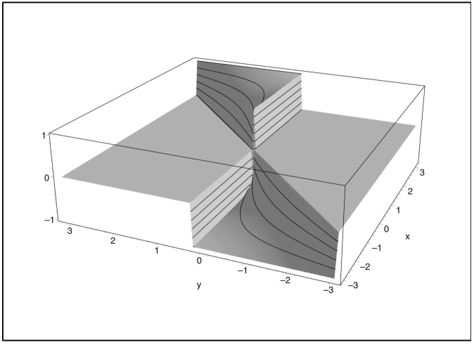
Figure 1: Green’s function $G(x,y)$ for $f(x)=\sin(x)$ and $\varepsilon=1$.

Lemma 5.

Let $u\in\mathrm{Dom}(L_{\varepsilon})$. Then $u\perp 1$ and $L_{\varepsilon}u=F$, if and only if

$$u(x)=TF(x)-\frac{1}{2\pi}\langle TF,1\rangle=(I-\frac{1}{2\pi}|1\rangle\langle 1|)TF(x)\qquad\text{and}\qquad F\perp 1.$$

Proof.

Suppose that $u\perp 1$ and $L_{\varepsilon}u=F$. Therefore, by (2.12),

$$0=\int_{-\pi}^{\pi}u(x)dx=\int_{-\pi}^{\pi}TF(x)+kdx=\langle TF,1\rangle+2\pi k$$

and so $2\pi k=-\langle TF,1\rangle$. This proves one direction of the implication. The other direction is trivial. ∎

Let $\tilde{D}=\mathrm{Dom}(L_{\varepsilon})\ominus\mathrm{span}\{1\}$. Then $L_{\varepsilon}$ has the block diagonal representation

$$L_{\varepsilon}=L_{\varepsilon}\upharpoonright_{\tilde{D}}\oplus 0\colon\tilde{D}\oplus\mathrm{span}\{1\}\to\mathrm{span}\{1\}^{\perp}\oplus\mathrm{span}\{1\}.$$

Let

$$\tilde{T}F(x)=TF(x)-\frac{1}{2\pi}\langle TF,1\rangle$$

for $F\in L^{2}(-\pi,\pi)\ominus\mathrm{span}\{1\}$ so that, by Lemma 5, $\tilde{T}\colon\mathrm{span}\{1\}^{\perp}\to\tilde{D}$. Then $(L_{\varepsilon}\upharpoonright_{\tilde{D}})^{-1}=\tilde{T}$ and, in particular, $0\not\in{\mathrm{spec}}(L_{\varepsilon}\upharpoonright_{\tilde{D}})$. Since $\tilde{T}$ is a rank-$1$ perturbation of $T\upharpoonright_{\mathrm{span}\{1\}^{\perp}}$ and the generalised singular value decomposition preserves any block structure of operators, we know the following.

Lemma 6.

The resolvent of $L_{\varepsilon}$ is in the $p$-Schatten class $\mathcal{C}_{p}$ if and only if $T\in\mathcal{C}_{p}$.

Given an $r>0$, we will denote

$$\mathcal{C}_{p>r}=\bigcap_{p>r}\mathcal{C}_{p}.$$

In order to find the Schatten properties of $T$ we consider below a generic lemma which, keeping the notation tidy, we formulate in $L^{2}(0,\pi)$. It can be easily seen that the interval $(0,\pi)$ can be replaced with any other bounded interval.

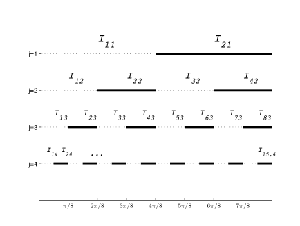
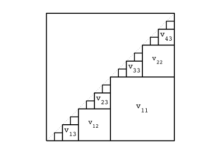
Figure 2: Left: For each fixed $j$ the intervals $I_{2k,j}$ and $I_{2k-1,j}$ are disjoint. Right: Illustration of the support of $v_{kj}(x,y)$.

Lemma 7.

Let $a,b\colon(0,\pi)\to{\mathbb{C}}$ be two continuous functions and denote by $v(x,y)=a(x)b(y)$. Let

$$S(u)(x)=\int_{0}^{x}v(x,y)u(y)dy.$$

If

$$v(x,y)=\left\{\begin{array}[]{ll}O(x^{-\alpha}),&\mbox{when}\quad(x,y)\to(0,0);\\ O((\pi-y)^{-\beta}),&\mbox{when}\quad(x,y)\to(\pi,\pi),\end{array}\right.$$

for some $0\leq\alpha,\beta<1/2$, then $S\in\mathcal{C}_{p>r(\alpha,\beta)}$ where

$$r(\alpha,\beta)=\max\{1/(1-\alpha),1/(1-\beta)\}.$$

Proof.

Let $\mathbb{1}_{ij}=\mathbb{1}_{I_{ij}}$ be the characteristic function of the interval $I_{ij}=[\frac{(i-1)\pi}{2^{j}},\frac{i\pi}{2^{j}})$ for $i=1,\dots,2^{j}$ and $j\in{\mathbb{N}}$. See Figure 2 (left). By construction, we have the pointwise equality

$$v(x,y)\mathbb{1}_{\Omega}(x,y)=\sum_{j=1}^{\infty}v_{j}(x,y),$$

where

$$v_{j}(x,y)=\sum_{k=1}^{2^{j-1}}a(x)\mathbb{1}_{2k,j}(x)b(y)\mathbb{1}_{2k-1,j}(y)=\sum_{k=1}^{2^{j-1}}v_{kj}(x,y)$$

and $\mathbb{1}_{\Omega}$ is the characteristic function of $\Omega=\{(x,y)\,|\,0<y<x<\pi\}$. See Figure 2 (right).

Let $S_{j}=\sum_{k=1}^{2^{j-1}}S_{kj}$ where

$$S_{kj}u(x)=|b\mathbb{1}_{2k-1,j}\rangle\langle a\mathbb{1}_{2k,j}|u(x)=\int_{0}^{\pi}v_{kj}(x,y)u(y)dy.$$

Since, for each fixed $j$, all the intervals indexed by $k$ are disjoint, this is a singular value decomposition for $S_{j}$. The $p$th Schatten class norm of $S_{kj}$ is

$$\alpha_{kj}:=\|S_{kj}\|_{p}=\|a\|_{L^{2}(I_{2k,j})}\|b\|_{L^{2}(I_{2k-1,j})}$$

for all $1\leq p\leq\infty$ (in particular, it is independent of $p$). Thus, if we prove that

(3.2) $$\sum_{j=1}^{\infty}\|S_{j}\|_{p}=\sum_{j=1}^{\infty}\left(\sum_{k=1}^{2^{j-1}}|\alpha_{kj}|^{p}\right)^{\frac{1}{p}}<\infty,$$

we would have that $S\in\mathcal{C}_{p}$ as the sum $S=\sum_{j=1}^{\infty}S_{j}$ would converge in the $p$th Schatten norm $\|\cdot\|_{p}$.

For $j\geq 2$ we can certainly separate the sum

$$S_{j}=\sum_{k=1}^{2^{j-2}}S_{kj}+\sum_{k=2^{j-2}}^{2^{j-1}}S_{kj}=S_{j}^{\ell}+S_{j}^{u}$$

and

$$S=S_{11}+\sum_{j=2}^{\infty}S_{j}^{\ell}+\sum_{j=2}^{\infty}S_{j}^{u}=S_{11}+S^{\ell}+S^{u},$$

so the proof will be complete (as was the case with (3.2)) if we can show

(3.3) $$\sum_{j=2}^{\infty}\|S_{j}^{\ell}\|_{p} <\infty\quad\mbox{for}\quad p>\frac{1}{1-\alpha}\quad\mbox{and}$$

(3.4) $$\sum_{j=2}^{\infty}\|S_{j}^{u}\|_{p} <\infty\quad\mbox{for}\quad p>\frac{1}{1-\beta}.$$

We will just prove (3.3), the proof of (3.4) being similar.

The hypotheses of the lemma guarantee that there exists a constant $c_{8}>0$ such that

$$|v(x,y)|\leq c_{8}x^{-\alpha}\quad\mbox{for all}\quad(x,y)\in\bigcup_{\tiny\begin{array}[]{c}j\geq 2\\ 1\leq k\leq 2^{j-2}\end{array}}I_{2k,j}\times I_{2k-1,j}.$$

Then, for $1\leq k\leq 2^{j-2}$,

(3.5) $$\alpha_{kj}^{2} =\int_{I_{2k,j}}\int_{I_{2k-1,j}}|v(x,y)|^{2}dxdy$$

$$\leq c_{8}\int_{I_{2k,j}}\int_{I_{2k-1,j}}x^{-2\alpha}dxdy=c_{8}\pi 2^{-j}\int_{\pi(2k-1)2^{-j}}^{\pi(2k)2^{-j}}x^{-2\alpha}dx$$

$$=c_{9}2^{-j}\left[\left(\frac{2k}{2^{j}}\right)^{1-2\alpha}-\left(\frac{2k-1}{2^{j}}\right)^{1-2\alpha}\right].$$

Letting $N=1/(1-2\alpha)$, so that $0\leq\alpha<1/2$ if and only if $N\geq 1$. We have that

$$1-r\leq\frac{1-r^{N}}{1+r^{N+1}}\quad\mbox{for all $0\leq r\leq 1$ and $N\geq 1$}.$$

Thus the right-hand side of (3.5) becomes

$$c_{9}2^{-j}\left(\frac{2k}{2^{j}}\right)^{\frac{1}{N}}\left[1-\left(\frac{2k-1}{2k}\right)^{\frac{1}{N}}\right]\leq c_{9}2^{-j(1+1/N)}\left(2k\right)^{\frac{1}{N}}\left[\frac{1-\frac{2k-1}{2k}}{1+\left(\frac{2k-1}{2k}\right)^{\frac{N-1}{N}}}\right]$$

$$=c_{9}2^{-j(1+1/N)}\left(2k\right)^{\frac{1}{N}}\left[\frac{1}{\left(2k\right)^{\frac{N-1}{N}}+\left(2k-1\right)^{\frac{N-1}{N}}}\right]\leq c_{9}2^{-j(1+1/N)}.$$

Therefore $\alpha_{kj}\leq c_{9}2^{-j(1+1/N)/2}$ for $1\leq k\leq 2^{j-2}$. Thus

$$\|S_{j}^{\ell}\|_{p}=\left(\sum_{k=1}^{2^{j-2}}\alpha_{kj}^{p}\right)^{\frac{1}{p}}\leq c_{9}\left(2^{j-2}2^{-jp(1+1/N)/2}\right)^{\frac{1}{p}}=c_{9}(2^{\frac{1}{p}})^{j(1-p(1+1/N)/2)}.$$

And so, $\sum_{j=1}^{\infty}\|S_{j}^{\ell}\|_{p}$ converges if $1-p(1+1/N)/2<0$, which is equivalent to $p>1/(1-\alpha)$. ∎

By virtue of this lemma we are able to prove the following theorem.

Theorem 8.

$T\in\mathcal{C}_{p>2/3}$.

Proof.

Let $\Omega^{\pm}=\{(x,y)\in{\mathbb{R}}^{2}:0<\pm y<\pm x<\pm\pi\}$. Let

$$G^{\pm}(x,y)=\pm\left(1-\frac{\psi(x)}{\psi(y)}\right)\mathbb{1}_{\Omega^{\pm}}(x,y).$$

Then $T=T^{+}+T^{-}$ where

$$T^{\pm}u(x)=\int_{-\pi}^{\pi}G^{\pm}(x,y)u(y)dy.$$

The proof reduces to showing that $T^{\pm}\in\mathcal{C}_{p>2/3}$. We shall only give the details for the case of $T^{+}$, the other case being analogous.

Set $T^{+}=T^{+}_{1}+T^{+}_{2}+T^{+}_{3}$ where

$$T^{+}_{j}u(x)=\int_{-\pi}^{\pi}G_{j}^{+}(x,y)u(y)dy\qquad\text{for}\qquad G_{j}^{+}(x,y)=G^{+}(x,y)\mathbb{1}_{\Omega_{j}^{+}}(x,y),$$

$$\Omega_{1}^{+}=\{0<x<y<\pi/2\},\qquad\Omega_{2}^{+}=[\pi/2,\pi]\times[0,\pi/2],$$

$$\text{and}\qquad\Omega_{1}^{+}=\{\pi/2<x<y<\pi\}.$$

We prove that each of the $T^{+}_{j}\in\mathcal{C}_{p>2/3}$.

Note that $T^{+}_{2}\in\mathcal{C}_{p>0}$ as it is of rank two. Let us show that $T^{+}_{1}\in\mathcal{C}_{p>2/3}$. Let

$$K_{1}^{+}(x,y)=\partial_{x}G(x,y)\mathbb{1}_{\Omega_{1}^{+}}(x,y)=\left\{\begin{array}[]{ll}\frac{\psi^{\prime}(x)}{\psi(y)},&\mbox{when}\quad(x,y)\in\Omega_{1}^{+};\\ 0,&\mathrm{otherwise}.\end{array}\right.$$

Then, for any $0<\alpha<1/2$,

$$T_{1}^{+}u(x) =\int_{0}^{\pi/2}\int_{0}^{x}K_{1}^{+}(z,y)u(y)dzdy$$

$$=\int_{0}^{x}z^{-\alpha}\int_{0}^{\pi/2}z^{\alpha}K_{1}^{+}(z,y)u(y)dydz=S_{1\alpha}^{+}(R_{1\alpha}^{+}[u])(x).$$

By virtue of Lemma 7, $S_{1\alpha}^{+}\in\mathcal{C}_{p>1/(1-\alpha)}$. On the other hand, by (2.5), (2.6) and (2.8), $|z^{\alpha}K_{1}^{+}(z,y)|\sim z^{\alpha-1}$ for $(z,y)\sim(0,0)$, so

$$\int_{0}^{\pi}\int_{0}^{\pi/2}|z^{\alpha}K_{1}^{+}(z,y)|^{2}dydz<\infty$$

whenever $\alpha>0$. Thus $R_{1\alpha}^{+}\in\mathcal{C}_{2}$. As $\alpha$ can be taken arbitrarily close to zero, $\|T_{1}^{+}\|_{p}\leq 2^{1/p}\|S^{+}_{1\alpha}\|_{q}\|R^{+}_{1\alpha}\|_{2}$ with $1/p=1/q+1/2$ and $q>1$ but arbitrarily close to one. Therefore $T^{+}_{1}\in\mathcal{C}_{p>2/3}$.

Arguing similarly for $T^{+}_{3}$ we set

$$K^{+}_{3}(x,y)=\partial_{y}G(x,y)\mathbb{1}_{\Omega_{3}^{+}}(x,y)=\left\{\begin{array}[]{ll}-\frac{\psi(x)\psi^{\prime}(y)}{\psi(y)^{2}},&\mbox{when}\quad(x,y)\in\Omega^{+}_{3};\\ 0,&\text{otherwise}.\end{array}\right.$$

Then, for any $0<\beta<1/2$,

$$T^{+}_{3}u(x) =-\int_{\pi/2}^{\pi}\int_{y}^{\pi}K_{3}^{+}(x,z)u(y)dzdy$$

$$=-\int_{\pi/2}^{\pi}K_{3}^{+}(x,z)(\pi-z)^{\beta}\left(\int_{\pi/2}^{z}(\pi-z)^{-\beta}u(y)dy\right)dz$$

$$=R_{3\beta}^{+}(S_{3\beta}^{+}[u])(x).$$

Once again, by Lemma 7, $S_{3\beta}^{+}\in\mathcal{C}_{p>1/(1-\beta)}$ and $|(\pi-z)^{\beta}K_{3}^{+}(x,z)|\sim(\pi-z)^{\beta-1}$ for $(x,z)\sim(\pi,\pi)$, so

$$\int_{0}^{\pi}\int_{\pi/2}^{\pi}|K_{3}^{+}(x,z)(\pi-z)^{\beta}|^{2}dzdx<\infty$$

whenever $\beta>0$. Thus $R_{3\beta}^{+}\in\mathcal{C}_{2}$. As $\beta$ can be taken arbitrarily close to zero, the proof follows in similar fashion as the previous case.∎

4 The forward-backward heat equation

By virtue of [2, Theorem 3.3], the spectrum of $L_{\varepsilon}$ is contained in the purely imaginary axis. If $iL_{\varepsilon}$ was similar to a self-adjoint operator, it would be the generator of a unitary one-parameter semigroup. In [9] it was shown that the latter is actually not the case for $f(x)=\sin(x)$. In this context we now examine more closely the evolution equation associated to $L_{\varepsilon}$ following the ideas of [5].

Let $T>0$. Consider the evolution problem

(B) $$\left\{\begin{aligned} &\partial_{t}u(t,x)+L_{\varepsilon}u(t,x)=0&\text{a.e. }(t,x)\in(0,T)\times(-\pi,\pi)\\ &u(t,\cdot)\in\mathrm{Dom}(L_{\varepsilon})&\forall t\in(0,T)\\ &u(0,x)=g(x)&\text{a.e. }x\in(-\pi,\pi).\end{aligned}\right.$$

We wish to define in a precise manner the notion of a solution of (B). If $L_{\varepsilon}\phi=i\lambda\phi$ for $\lambda\in\mathbb{R}$ and $g(x)=\phi(x)$, then formally we have a global solution of (B) given by $u(t,x)=e^{-i\lambda t}\phi(x)$ for any $T>0$. In an analogous fashion, we can generate solutions which are global whenever $g$ is a finite linear combination of eigenfunctions of $L_{\varepsilon}$.

We will denote the space of admissible trajectories in which the solutions of (B) lie by

$$\mathcal{AT}_{T}:=W^{1,2}_{2,\mathrm{loc}}\big{(}(0,T)\times[(-\pi,0)\cup(0,\pi)]\big{)}\cap C\left([0,T);L^{2}(-\pi,\pi)\right).$$

Here and below we follow closely the notation of [13], where $W^{r,k}_{2}(\Omega)$ is the parabolic Sobolev space for an open region $\Omega\subset\mathbb{R}^{2}$ of function with derivatives in the $x$-variable up to order $k$ and derivatives in the $t$-variable up to order $r$. The space $W^{r,k}_{2,\mathrm{loc}}(\Omega)$ is defined by saying $v\in W^{r,k}_{2,\mathrm{loc}}(\Omega)$ iff $\phi v\in W^{r,k}_{2}(\mathbb{R}^{2})$ for all smooth cut-off functions $\phi$ whose support is inside a compact proper subset of $\Omega$. Note that if $v\in\mathcal{AT}_{T}$, then $\partial_{t}v+L_{\varepsilon}v\in L^{2}((0,T)\times(-\pi,\pi))$. Here and below, expressions involving partial derivatives will always mean partial derivatives in the distributional (Sobolev) sense.

By a solution of (B) we mean $u\in\mathcal{AT}_{T}$ satisfying all conditions in (B) for some $T>0$.

To simplify notation, we will denote functions and their corresponding restrictions to subdomains (or extensions to larger domains) with the same letter. Extensions to larger domains are assumed to be “up to a set of measure zero”.

In the following lemma it is crucial that $I_{0}\subset(0,\pi)$, however note that there are no restrictions on the position of $J$ relative to $t=0$.

Lemma 9.

Let $f\in C^{k}(\mathbb{R})$ for some $k\in\mathbb{N}$. Let $I_{0}\subset\overline{I}_{0}\subset(0,\pi)$ and $J\subset\mathbb{R}$ be two open intervals. If $v\in W^{1,2}_{2,\mathrm{loc}}(J\times I_{0})$ is such that $\partial_{t}v+\ell_{\varepsilon}v=0$, then $v\in W^{1,2+k}_{2}(V)$ for any $V\subset J\times I_{0}$.

Proof.

The proof follows closely that of [13, Corollary 2.4.1]. Let $V_{0},\,V_{1}$ be two open sets, such that $V_{0}\subset\overline{V_{0}}\subset V_{1}\subset\overline{V_{1}}\subset J\times I_{0}$. Consider a cutoff function associated to $V_{0}$ and $V_{1}$: $\zeta\in C^{\infty}_{c}(\mathbb{R}^{2})$, such that $\zeta(t,x)=1$ for $(t,x)\in V_{0}$ and $\zeta(t,x)=0$ for $(t,x)\in\mathbb{R}^{2}\setminus V_{1}$. A straightforward calculation yields

$$(\partial_{t}+\ell_{\varepsilon})(\zeta v)=[v(\partial_{t}+\ell_{\varepsilon})\zeta]+[2\varepsilon f\zeta^{\prime}v^{\prime}].$$

Elementary properties of the parabolic Sobolev spaces ensure that the first summing term on the right lies in $W^{1,2}_{2}(\mathbb{R}^{2})$ and the second one lies in $W^{1,1}(\mathbb{R}^{2})$. Note that here $k\geq 1$ is required. Thus the whole expression lies in $W^{0,1}_{2}(\mathbb{R}^{2})$.

By virtue of [13, Corollary 2.3.3], $\zeta v\in W^{1,3}_{2}(\mathbb{R}^{2})$. As $\zeta=1$ in $V_{0}$, the parabolic Sobolev embedding theorem ensures that $u\in W^{1,3}(V_{0})$. This shows the lemma for $k=1$. If $k>1$, on the other hand, the argument can be repeated until we get $v\in W^{1,2+k}_{2}(V)$. ∎

We now combine Lemma 9 with [13, Theorem 2.2.6], in order to get the following non-existence result for (B).

Theorem 10.

Let $f\in C^{k}(\mathbb{R})$ for some $k\in\mathbb{N}$. Let $g\in L^{2}(-\pi,\pi)$. If there exists a solution $u\in\mathcal{AT}_{\delta}$ of (B) for some $\delta>0$, then $g\in C^{\kappa}(I_{0})$ for any $I_{0}\subset\overline{I_{0}}\subset(0,\pi)$ where

$$\kappa=\left\{\begin{aligned} &\frac{k-1}{2}&k\ \text{odd}\\ &\frac{k}{2}&k\ \text{even}.\end{aligned}\right.$$

Proof.

Let $J=(-\delta,\delta)$. The idea of the proof is to “glue” together $u$ with a solution $u^{d}$ of a Dirichlet evolution problem associated to $L_{\varepsilon}$ in $(-\delta,0)\times I_{0}$ and observe that the “seam” of this gluing is $g(x)$.

Let $u^{d}(t,x)$ for $(t,x)\in(0,\delta)\times I_{0}$ be a solution of the parabolic problem

(4.1) $$\left\{\begin{aligned} &\partial_{t}u^{d}-L_{\varepsilon}u^{d}=0&\forall(t,x)\in(0,\delta)\times I_{0}\\ &u^{d}(t,\min I_{0})=u^{d}(t,\max I_{0})=0&\forall t\in(0,\delta)\\ &u^{d}(0,x)=g(x)&\forall x\in I_{0}.\end{aligned}\right.$$

Since $f$ is positive definite in $I_{0}$, (4.1) has a unique (actually global in time) solution. By virtue of Lemma 9,

(4.2) $$u^{d},u\in W^{1,2+k}_{2}((0,\delta)\times I_{0}).$$

Let

$$v(t,x)=\left\{\begin{aligned} &u^{d}(-t,x)&-\delta<t\leq 0,\,x\in I_{0}\\ &u(t,x)&0\leq t<\delta,\,x\in I_{0}.\end{aligned}\right.$$

Note that the change in the sign for $t$ ensures that in the region $(-\delta,0)\times I_{0}$, $\partial v_{t}+L_{\varepsilon}v=0$. By construction $v\in L^{2}(J\times I_{0})$. We show that $v\in W^{1,2}_{2}(J\times I_{0})$.

Let us verify firstly that $\partial_{t}v\in L^{2}(J\times I_{0})$. Let

$$h(t,x)=\left\{\begin{aligned} &-\partial_{t}u^{d}(-t,x)&-\delta<t<0,\,x\in I_{0}\\ &\partial_{t}u(t,x)&0<t<\delta,\,x\in I_{0}.\end{aligned}\right.$$

By construction $h\in L^{2}(J\times I_{0})$. We now show that $\partial_{t}v=h$. For almost every $x\in I_{0}$,

$$v(\cdot,x)\in C(J)\cap\left[W^{1}_{2}(-\delta,0)\cup W^{1}_{2}(0,\delta)\right].$$

Then $\partial_{t}v(\cdot,x)=h(\cdot,x)\in L^{2}(J)$ for almost every $x\in I_{0}$. Thus

$$\int_{J}h(t,x)\phi(t)dt=-\int_{J}v(t,x)\partial_{t}\phi(t)dt\qquad\forall\phi\in C^{\infty}_{c}(J)$$

for almost every $x\in I_{0}$. Hence

$$\int_{I_{0}}\int_{J}h(t,x)\phi(t,x)dt\,dx=-\int_{I_{0}}\int_{J}v(t,x)\partial_{t}\phi(t,x)dt\,dx\qquad\forall\phi\in C^{\infty}_{c}(J\times I_{0}),$$

so that $\partial_{t}v=h\in L^{2}(J\times I_{0})$.

Now let us prove that $\partial_{x}v\in L^{2}(J\times I_{0})$. Let

$$k(t,x)=\left\{\begin{aligned} &\partial_{x}u^{d}(-t,x)&-\delta<t<0,\,x\in I_{0}\\ &\partial_{x}u(t,x)&0<t<\delta,\,x\in I_{0}.\end{aligned}\right.$$

Then $k\in L^{2}(J\times I_{0})$. Let us show that $\partial_{x}u=k$. Note that $u^{d}(-t,\cdot),u(t,\cdot)\in C^{2}(I_{0})$ for all $t\in(0,\delta)$ as a consequence of (4.2). Hence,

$$\int_{I_{0}}k(t,x)\phi(x)dx=-\int_{I_{0}}v(t,x)\partial_{x}\phi(x)dx\qquad\forall\phi\in C^{\infty}_{c}(I_{0})$$

for all $t\in J\setminus\{0\}$. Then

$$\int_{I_{0}}\int_{J}k(t,x)\phi(t,x)dt\,dx=-\int_{I_{0}}\int_{J}v(t,x)\partial_{x}\phi(t,x)dt\,dx\qquad\forall\phi\in C^{\infty}_{c}(J\times I_{0}).$$

Hence $\partial_{x}v=k\in L^{2}(J\times I_{0})$.

The proof that $\partial_{xx}v\in L^{2}(J\times I_{0})$ is similar. Note that here is crucial that $k\geq 1$. Hence $v\in W^{1,2}_{2}(J\times I_{0})$ as needed.

We complete the proof of the theorem as follows. By Lemma 9, $v\in W^{1,2+k}_{2}(J\times I_{0})$. Since $g(x)=v(0,x)$, taking $r=1$ and the “$k$” of the theorem as “$2+k$” in [13, Theorem 2.2.6], we get for $\kappa<\frac{1+k}{2}$ (which is equivalent to $\frac{2\kappa+1}{2(2+k)}+\frac{1}{2}<1$ in the mentioned theorem) that $g\in C^{\kappa}(I_{0})$. ∎

One relevant question in the context of this theorem is the existence of solution of (B) (for $T$ sufficiently small), if $\mathrm{supp}(g)\subset J\subset\overline{J}\subset(-\pi,0)$. A positive answer would certainly be of interest. In this respect the “barrier” at $x=0$ may prevent this solution propagating from $(-\pi,0)$ to $(0,\pi)$ and make it lose its regularity.

5 Basis properties of the eigenfunctions of $L_{\varepsilon}$

With Theorem 10 at hand and the “diagonalisation” lemma below, we can establish properties of the set of eigenfunctions of $L_{\varepsilon}$. First, however, we deal with one piece of unfinished business from [2]. A proof of the second statement in the following theorem by different methods can be found in [5, Proposition 5.5] for the case $f(x)=\sin(x)$.

Theorem 11.

Suppose that $f$ satisfies conditions 1-4 from Section 1. The operator $L_{\varepsilon}$ has infinitely many eigenvalues. Moreover, all these eigenvalues are algebraically simple. Consequently, the eigenspaces of $L_{\varepsilon}$ contain only eigenfunctions and no associated functions.

Proof.

Following the notation in [2], we introduce the meromorphic function

(5.1) $$\rho(z)=\frac{\phi(\pi;-iz^{2})}{\phi(\pi;iz^{2})}=\frac{\Pi_{n=1}^{\infty}\left(1-\frac{z^{2}}{\alpha_{n}^{2}}\right)}{\Pi_{n=1}^{\infty}\left(1+\frac{z^{2}}{\alpha_{n}^{2}}\right)}=\prod_{n=1}^{\infty}\frac{1-\frac{z^{2}}{\alpha_{n}^{2}}}{1+\frac{z^{2}}{\alpha_{n}^{2}}}.$$

Here $\phi(x;\lambda)$ is the unique solution of the differential equation $i\ell_{\epsilon}\phi=\lambda\phi$ satisfying $\phi(0;\lambda)=1$. The sequence $(\alpha_{n})$ consists entirely of positive numbers and its asymptotic behaviour is $\alpha_{n}=O(n)$ as $n\to\infty$, so it grows sufficiently rapidly to ensure the convergence of the products on the right hand side. It was proved in [2] that $\lambda$ is an eigenvalue of $iL_{\epsilon}$ if and only if $\lambda=-iz^{2}$ for $z\in\mathbb{C}$ such that $\rho(z)=1$. Moreover it was shown that $|\rho(z)|=1$ on, and only on, the lines $\arg(z)\equiv\pi/4$ (modulo $\pi/2$).

For the first part of the theorem it suffices to show that there exist infinitely many $r\in\mathbb{R}$ such that $\rho(r\exp(i\pi/4))=1$. To this end we put $\rho(r\exp(i\pi/4))=\mu(r)=\exp(i\Theta(r))$ which maps $\mathbb{R}$ smoothly into the unit circle, $\mathbb{T}$. Here the function $\Theta(r)$ is chosen by picking a branch of the logarithm in the expression

$$i\Theta(r) =\log(\mu(r))=\sum_{n=1}^{\infty}\left\{\log\left(1-i\frac{r^{2}}{\alpha_{n}^{2}}\right)-\log\left(1+i\frac{r^{2}}{\alpha_{n}^{2}}\right)\right\}$$

$$=2i\sum_{n=1}^{\infty}\arg\left(1-i\frac{r^{2}}{\alpha_{n}^{2}}\right).$$

For convenience we choose the branch $[-\pi,\pi)$ and observe that all summations in the above converge as a consequence of the convergence of (5.1). We now show that $\rho$ passes through any point of $\mathbb{T}$ (including the needed value 1) an infinite number of times as $|r|$ increases.

The meromorphic function $\rho(1/z)$ has an essential singularity at the origin. Therefore, in any neighbourhood of $0$, $\rho(1/z)$ assumes each complex number, with the possible exception of one, infinitely many times. Since $|\rho(z)|=1$ only on the rays $\arg(z)\equiv\pi/4$ (modulo $\pi/2$) and $\rho(\overline{z})=\overline{\rho(z)}$, necessarily $\mu(r)$ assumes any value of $\mathbb{T}$, with the possible exception of one, infinitely many times for $r\in\mathbb{R}$. Now

$$\partial_{r}\mu(r)=i\Theta^{\prime}(r)\exp\left(i\Theta(r)\right).$$

Here $\Theta^{\prime}(r)$ is defined as the derivative from the “right”, if $r$ is such that $\Theta(r)=-\pi$. Differentiation yields

$$\Theta^{\prime}(r)=-4r\sum_{n=1}^{\infty}\alpha_{n}^{-2}\frac{1}{1+\frac{r^{4}}{\alpha_{n}^{4}}},$$

where the summation is convergent, once again, due to the growth of $\alpha_{n}$ at infinity. This shows that $\partial_{r}\mu(r)$ only vanishes at $r=0$. Hence, there are no exceptions in the values that $\mu(r)$ attains on $\mathbb{T}$ an infinite number of times, which means that $\rho(z)=1$ infinitely many times on the ray $z=r\exp(i\pi/4)$.

In order to achieve the second part of the theorem we follow Kato [12, Chapter III, §5]. It suffices to show that the resolvent $(L_{\varepsilon}-\lambda)^{-1}$ has only algebraically simple poles. For this we employ an expression for the Green’s function found in [3, §3]. We require, in addition to the solution $\phi(x;\lambda)$, a second solution $\psi(x;\lambda)$ which is analytic in $\lambda$ for $x\neq 0$, satisfies $\psi(\pm\pi;\lambda)=0$, and has the Wronskian property

$$\left|\begin{array}[]{cc}\phi(x;\lambda)&\psi(x;\lambda)\\ p(x)\phi^{\prime}(x;\lambda)&p(x)\psi^{\prime}(x;\lambda)\end{array}\right|\equiv 1.$$

Here $p$ is the coefficient introduced in (2.2). According to [3, (3.1)-(3.6)], for any $F\in L^{2}(-\pi,\pi)$, $u=(L_{\varepsilon}-\lambda)^{-1}F$ is given by

$$u(x;\lambda) =\phi(x;\lambda)\int_{x}^{\pi}\psi(t;\lambda)\frac{p(t)}{\epsilon f(t)}F(t)dt+\psi(x;\lambda)\int_{0}^{x}\phi(t;\lambda)\frac{p(t)}{\epsilon f(t)}F(t)dt$$

$$\qquad+\hskip 14.22636pt\frac{\phi(x;\lambda)\phi(-\pi;\lambda)}{\phi(\pi;\lambda)-\phi(-\pi;\lambda)}{\displaystyle\int_{-\pi}^{\pi}\psi(t;\lambda)\frac{p(t)}{\epsilon f(t)}F(t)dt}.$$

The only singularities in this expression come from the zeros of the denominator, which in turn are the zeros of

$$1-\frac{\phi(-\pi;\lambda)}{\phi(\pi;\lambda)}=1-\rho(z).$$

Indeed, recall from [2] that $\phi(-\pi;\lambda)=\phi(\pi;-\lambda)$. Moreover, multiplicities coincide except at $z=0$, where a double root in terms of $z$ is a simple root in terms of $\lambda$.

Apart from the double root at $z=0$, all the roots of $\rho(z)=1$ are simple. They lie on the lines $\arg(z)\equiv\pi/4$ (modulo $\pi/2$) where $|\rho(z)|=1$, and on these lines the phase of $\rho$ has been shown to be non-stationary, except at $z=0$. Thus $(L_{\varepsilon}-\lambda)^{-1}$ has only simple poles as needed. ∎

In the sequel we follows [6, Section 3.3-3.4] for the notions of conditional and unconditional basis. Recall that if $\{\phi_{n}\}$ is a conditional basis on a Hilbert space, there exists a dual set $\{\phi_{n}^{*}\}$ such that $\{\phi_{n},\phi_{n}^{*}\}$ is bi-orthogonal in the sense that $\langle\phi_{n},\phi_{m}^{*}\rangle=\delta_{nm}$ and for all $g\in\mathcal{H}$,

$$\|g-\sum_{n=1}^{k}\widehat{g}(n)\phi_{n}\|\to 0\qquad k\to\infty$$

where the “generalised Fourier coefficients” $\widehat{g}(n)=\langle g,\phi_{n}^{*}\rangle$.

Lemma 12.

Let $M:\operatorname{Dom}(M)\longrightarrow\mathcal{H}$ be a closed operator on the infinite-dimensional Hilbert space $\mathcal{H}$. Assume that the resolvent of $M$ is compact and denote by $\mu_{n}\in\mathbb{C}$ the eigenvalues of $M$ with corresponding eigenfunctions $\phi_{n}\not=0$, $M\phi_{n}=\mu_{n}\phi_{n}$. If $\{\phi_{n}\}_{n=1}^{\infty}$ is a conditional basis, then $\operatorname{Dom}(M)=\mathcal{D}$ where

(5.2) $$\mathcal{D}=\{g\in\mathcal{H}:\sum_{n=1}^{k}\mu_{n}\widehat{g}(n)\phi_{n}\to h\in\mathcal{H}\}$$

and $Mg=h$ for $g\in\mathcal{D}$.

Proof.

Let $g\in\mathcal{D}$ and $g_{k}=\sum_{n=1}^{k}\widehat{g}(n)\phi_{n}$. Then $g_{k}\in\operatorname{Dom}(M)$, $g_{k}\to g$ and $M(g_{k}-g_{j})\to 0$ as $j,k\to\infty$. Since $M$ is closed, then $g\in\operatorname{Dom}(M)$ and $Mg=\lim_{k\to\infty}Mg_{k}$.

Conversely, let $g\in\operatorname{Dom}(M)$. Then $g=(M-\mu)^{-1}z$ for a suitable $\mu\not=\mu_{n}$ and $z\in\mathcal{H}$. Note that the spectrum of $(M-\mu)^{-1}$ is $\{\frac{1}{\mu_{n}-\mu}\}\cup\{0\}$ and $(M-\mu)^{-1}\phi_{n}=\frac{1}{\mu_{n}-\mu}\phi_{n}$. Also

$$\langle(M^{*}-\overline{\mu})^{-1}\phi^{*}_{n},\phi_{m}\rangle=\langle\phi^{*}_{n},(M-\mu)^{-1}\phi_{m}\rangle=\frac{\delta_{nm}}{\overline{\mu_{n}}-\overline{\mu}},$$

so $(M^{*}-\overline{\mu})^{-1}\phi_{n}^{*}=\frac{1}{\overline{\mu_{n}}-\overline{\mu}}\phi_{n}^{*}$. Hence

$$\widehat{g}(n)=\langle g,\phi^{*}_{n}\rangle=\langle(M-\mu)^{-1}z,\phi^{*}_{n}\rangle=\frac{\widehat{z}(n)}{\mu_{n}-\mu}.$$

Thus $(\mu_{n}-\mu)\widehat{g}(n)=\widehat{z}(n)$. Since both $\|z-\sum_{n=1}^{k}\widehat{z}(n)\phi_{n}\|\to 0$ and $\|\mu g-\mu g_{k}\|\to 0$, then $\sum_{n=1}^{k}\mu_{n}\widehat{g}(n)\phi_{n}\to h$ for some $h\in\mathcal{H}$. Moreover $h=z+\mu g=Mg$. ∎

Assume now that $\{\phi_{n}\}$ is an unconditional basis of $\mathcal{H}$. Then the norm generated by $\{\phi_{n}^{*}\}$ is equivalent to the norm of $\mathcal{H}$. That is, there are positive constants $0<a\leq b<\infty$, such that

(5.3) $$a\|g\|^{2}\leq\sum|\hat{g}(n)|^{2}\leq b\|g\|^{2}\qquad\qquad\forall g\in\mathcal{H}.$$

See for example [6, Theorem 3.4.5]. Consider the case $M=L_{\varepsilon}$ and fix the eigenfunctions such that $L_{\varepsilon}\phi_{n}=i\lambda_{n}\phi_{n}$ for $\lambda_{n}\in\mathbb{R}$ the corresponding rotated eigenvalues.

The following statement is a consequence of Theorem 10. The hypothesis on the degree of smoothness of $f$ is only present here in order to invoke the latter. Most likely the conclusion will also hold true for less regular $f$, but the treatment of this case will require an analysis beyond the scope of the present paper.

Theorem 13.

If $f\in C^{7}(\mathbb{R})$, the eigenfunctions of $L_{\varepsilon}$ do not form an unconditional basis.

Proof.

Assume, for a contradiction, that $\{\phi_{n}\}$ is an unconditional basis. Let

$$h(x)=\left\{\begin{array}[]{ll}4x/\pi&0<x<\pi/4\\ -8x^{2}/\pi^{2}+8x/\pi-1/2&\pi/4<x<3\pi/4\\ -4(x-\pi)/\pi&3\pi/4<x<\pi\\ \text{extend to an odd function}&-\pi<x<0.\end{array}\right.$$

Then $h^{\prime}\in\mathrm{AC}(-\pi,\pi)$, $h\not\in H^{3}(-\pi,\pi)$ and $h\in\operatorname{Dom}(L_{\varepsilon})$ (by virtue of the characterisation of $\operatorname{Dom}(L_{\varepsilon})$ given in Section 2). For $k\in\mathbb{N}$, let

$$u_{k}(t,x)=\sum_{n=-k}^{k}e^{-i\lambda_{n}t}\widehat{h}(n)\phi_{n}(x).$$

The fact that $f\in C^{7}(\mathbb{R})$ together with a bootstrap argument yield $\partial_{x}^{8}\phi_{n}\in\mathrm{AC}_{\mathrm{loc}}((-\pi,0)\cup(0,\pi))$ for all $n\in\mathbb{N}$. Hence $u_{k}\in\mathcal{AT}_{T}$ for all $T>0$. Moreover, $u_{k}$ is a solution of (B) with $g=h_{k}=\sum_{n=-k}^{k}\widehat{h}(n)\phi_{n}$. Below we show that the limit $u:=\lim_{k\to\infty}u_{k}$ exists in a suitable sense, $u\in\mathcal{AT}_{T}$ for all $T>0$ and $u$ is a solution of (B) with $g=h$. This would immediately complete the proof, as Theorem 10 then implies the contradictory statement $h\in C^{3}(-\pi,\pi)$.

Since $h\in L^{2}(-\pi,\pi)$,

$$\sum_{n=-\infty}^{\infty}|\widehat{h}(n)|^{2}<\infty.$$

By virtue of (5.3), it follows that $\{u_{k}(t,\cdot)\}_{k}$ is a Cauchy sequence in $L^{2}(-\pi,\pi)$ for all $t\in\mathbb{R}$. Then $\{u_{k}(t,\cdot)\}_{k}$ converge in $L^{2}(-\pi,\pi)$ to a limit, $u(t,\cdot)$. This convergence is uniform in $t$, so $\{u_{k}\}_{k}$ converges in $L^{2}([0,T]\times(-\pi,\pi))$ to $u$ and $u\in C([0,T),L^{2}(-\pi,\pi))$ for all $T>0$. We show that $u\in W^{1,2}_{2,\mathrm{loc}}\big{(}(0,T)\times[(-\pi,0)\cup(0,\pi)]$ in three further steps.

According to our assumption, the representation of $\operatorname{Dom}(L_{\varepsilon})$ given by (5.2) holds true. Then

(5.4) $$\sum_{n=-\infty}^{\infty}|\mu_{n}\widehat{h}(n)|^{2}<\infty,\qquad\mu_{n}=i\lambda_{n}.$$

From (5.3) and (5.4) it follows that $\{\partial_{t}u_{k}(t,\cdot)\}_{k}$ is a Cauchy sequence in $L^{2}(-\pi,\pi)$ for all $t\in\mathbb{R}$. Then $\{\partial_{t}u_{k}\}_{k}$ converges in $L^{2}([0,T]\times(-\pi,\pi))$ to the distributional derivative $\partial_{t}u$, so that $\partial_{t}u\in L^{2}([0,T]\times(-\pi,\pi))$.

Let us now show that $\partial_{x}u$ is in $L^{2}_{\mathrm{loc}}\big{(}(0,T)\times[(-\pi,0)\cup(0,\pi)]\big{)}$. To this end we use the differential equation in (B). Let $\zeta\colon\mathbb{R}\times\mathbb{R}\to\mathbb{R}$ be a smooth function whose support is contained in $(0,T)\times[(-\pi,0)\cup(0,\pi)]$. For any $v\in\mathcal{AT}_{T}$ satisfying $(\partial_{t}+L_{\varepsilon})(v)=0$,

(5.5) $$(\partial_{t}+\ell_{\varepsilon})(\zeta v)=v(\partial_{t}+\ell_{\varepsilon})(\zeta)+2\varepsilon f\zeta^{\prime}v^{\prime}.$$

Multiplying (5.5) by $\zeta\overline{v}=\overline{\zeta v}$ and adding the result to its complex conjugate gives

$$\varepsilon(f(\zeta v)^{\prime})^{\prime}\zeta\overline{v}+\varepsilon(f(\zeta\overline{v})^{\prime})^{\prime}{\zeta v} =2\zeta|v|^{2}(\partial_{t}+\ell_{\varepsilon})(\zeta)+2\varepsilon f\zeta^{\prime}v^{\prime}\zeta\overline{v}+2\varepsilon f\zeta^{\prime}\overline{v^{\prime}}\zeta v$$

$$\quad-\partial_{t}|\zeta v|^{2}-\partial_{x}|\zeta v|^{2}.$$

Integrating in the spatial variable, integrating by parts and Cauchy-Schwarz inequality, lead to the estimate

$$\left|2\varepsilon\int_{-\pi}^{\pi}f(x)|(\zeta v)^{\prime}(t,x)|^{2}dx\right|$$

$$\leq c_{10}\left(\int_{-\pi}^{\pi}|v(t,x)|^{2}dx+\int_{-\pi}^{\pi}|\partial_{t}v(t,x)|^{2}dx+\int_{-\pi}^{\pi}|(\zeta v)^{\prime}(t,x)v(t,x)|dx\right)$$

$$\leq\left(c_{10}+\frac{c_{10}}{\delta}\right)\int_{-\pi}^{\pi}|v(t,x)|^{2}dx+c_{10}\int_{-\pi}^{\pi}|\partial_{t}v(t,x)|^{2}dx+\delta c_{10}\int_{-\pi}^{\pi}|(\zeta v)^{\prime}(t,x)|^{2}dx$$

for $\delta>0$. Here and below $c_{j}>0$ are constants which only depend on $\varepsilon$, $\zeta$ and $f$. Choosing $\delta>0$ sufficiently small enables us to move the last term on the right-hand side to the left. Integrating in $t$ yields

(5.6) $$\int_{0}^{T}\!\!\int_{-\pi}^{\pi}\!\!|(\zeta v)^{\prime}(t,x)|^{2}dx\,dt\leq c_{11}\!\!\left(\int_{0}^{T}\!\!\int_{-\pi}^{\pi}\!\!|v(t,x)|^{2}dx\,dt+\int_{0}^{T}\!\!\int_{-\pi}^{\pi}\!\!|\partial_{t}v(t,x)|^{2}dx\,dt\right)\!\!.$$

Since $u_{k}-u_{j}\in\mathcal{AT}_{T}$ and $(\partial_{t}+\ell_{\varepsilon})(u_{k}-u_{j})=0$ for any $k,j\in\mathbb{N}$, on applying (5.6) with $v=u_{k}-u_{j}$ we obtain an estimate where $c_{11}$ is independent of $k$ and $j$. Since $\{u_{k}\}$ and $\{\partial_{t}u_{k}\}$ are Cauchy sequences, we conclude that also $\{\partial_{x}(\zeta u_{k})\}_{k}$ is a Cauchy sequence in $L^{2}([0,T]\times(-\pi,\pi))$ for each fixed $\zeta$ whose support is contained in $(0,T)\times[(-\pi,0)\cup(0,\pi)]$. Thus $\partial_{x}u\in L^{2}_{\mathrm{loc}}\big{(}(0,T)\times[(-\pi,0)\cup(0,\pi)]\big{)}$.

The equation (5.5) implies that $\{\partial_{x}^{2}(\zeta u_{k})\}_{k}$ is also a Cauchy sequence and, by an analogous reasoning as before, $\partial_{x}^{2}u\in L^{2}_{\mathrm{loc}}\big{(}(0,T)\times[(-\pi,0)\cup(0,\pi)]\big{)}$. Thus $u\in\mathcal{AT}_{T}$ for any finite $T>0$. Moreover, since $u_{k}$ solves (B) with initial condition $h_{k}$, Lemma 4 implies that $u$ solves (B) with initial condition $h$. ∎

References

- [1] E S Benilov, S B G O’Brien, and I A Sazonov, A new type of instability: explosive disturbances in a liquid film inside a rotating horizontal cylinder, J. Fluid Mech. 497, 201–224 (2003).
- [2] L Boulton, M Levitin and M Marletta, On a class of non-self-adjoint periodic eigenproblems with boundary and interior singularities, J. Diff. Eq. 249, 3081–3098 (2010).
- [3] L Boulton, M Levitin and M Marletta, On a class of non-self-adjoint periodic boundary value problems with discrete real spectrum. Transl. AMS 231 59-66 (2010).
- [4] M Chugunova and D Pelinovsky, Spectrum of a non-self-adjoint operator associated with the periodic heat equation, J. Math. Anal. Appl. 342, 970–988 (2008).
- [5] M Chugunova, I Karabash and S Pyatkov, On the nature of ill-posedness of the forward-backward heat equation, Int. Equ. Op. Theo. 65, 319–344 (2009).
- [6] E B Davies, Linears Operators and their Spectra, Cambridge University Press, Cambridge (2007).
- [7] E B Davies, Spectral Theory and Differential Operators, Cambridge University Press, Cambridge (1995).
- [8] E B Davies, An indefinite convection-diffusion operator, LMS J. Comp. Math. 10, 288-306 (2007).
- [9] E B Davies and J Weir, Convergence of eigenvalues for a highly non-self-adjoint differential operator, Bull. LMS 42, 237â??249 (2010).
- [10] N Dunford and J Schwartz, Linear Operators, part II: Spectral Theory, Intertscience, New York (1957).
- [11] I Gohberg and M Krein, Introduction to the theory of linear non-selfadjoint operators, Translation of Mathematical Monographs 18, AMS, Providence (1969).
- [12] T Kato, Perturbation Theory for Linear Operators, Springer-Verlag, Berlin (1980).
- [13] N V Krylov, Lectures on Elliptic and Parabolic equations in Sobolev Spaces, Graduate Studies in Mathematics 96, AMS, Providence (2008).
- [14] J Weir, An indefinite convection-diffusion operator with real spectrum, Appl. Math. Letters 22 280-283 (2009).
- [15] J Weir, Correspondence of the eigenvalues of a non-self-adjoint operator to those of a self-adjoint operator, Mathematika 56 323-338 (2010).
- [16] J Weir, PhD Thesis. King’s College London (2010).