The Fundamental Surface of Quad Lenses

Abstract

In a quadruply imaged lens system the angular distribution of images around the lens center is completely described by three relative angles. We show empirically that in the three dimensional space of these angles, spanning $180^{\circ}\times 180^{\circ}\times 90^{\circ}$, quads from simple two-fold symmetric lenses of arbitrary radial density profile and arbitrary radially dependent ellipticity or external shear define a nearly invariant two dimensional surface. We give a fitting formula for the surface using SIS+elliptical lensing potential. Various circularly symmetric mass distributions with shear up to $\gamma\sim 0.4$ deviate from it by typically, rms$~{}\sim 0.1^{\circ}$, while elliptical mass distributions with ellipticity of up to $e\sim 0.4$ deviate from it by rms$~{}\sim 1.5^{\circ}$. The existence of a near invariant surface gives a new insight into the lensing theory and provides a framework for studying quads. It also allows one to gain information about the lens mass distribution from the image positions alone, without any recourse to mass modeling. As an illustration, we show that about 3/4 of observed galaxy-lens quads do not belong to this surface within observational error, and so require additional external shear or substructure to be modeled adequately.

1 Introduction

Recovering projected mass distribution of galaxies and clusters given the images of lensed background sources is an important problem, and much effort has been devoted to lens mass modeling over the last couple of decades. In this paper we show that useful information about the lensing object can be obtained without any recourse to mass modeling. We work exclusively with quadruply imaged lens systems (the fifth central image is usually not detected and is not part of the analysis), and more specifically, with the angular distribution of the four point-like images around the lens center, that was introduced in Williams et al. (2008). We do not consider image fluxes.

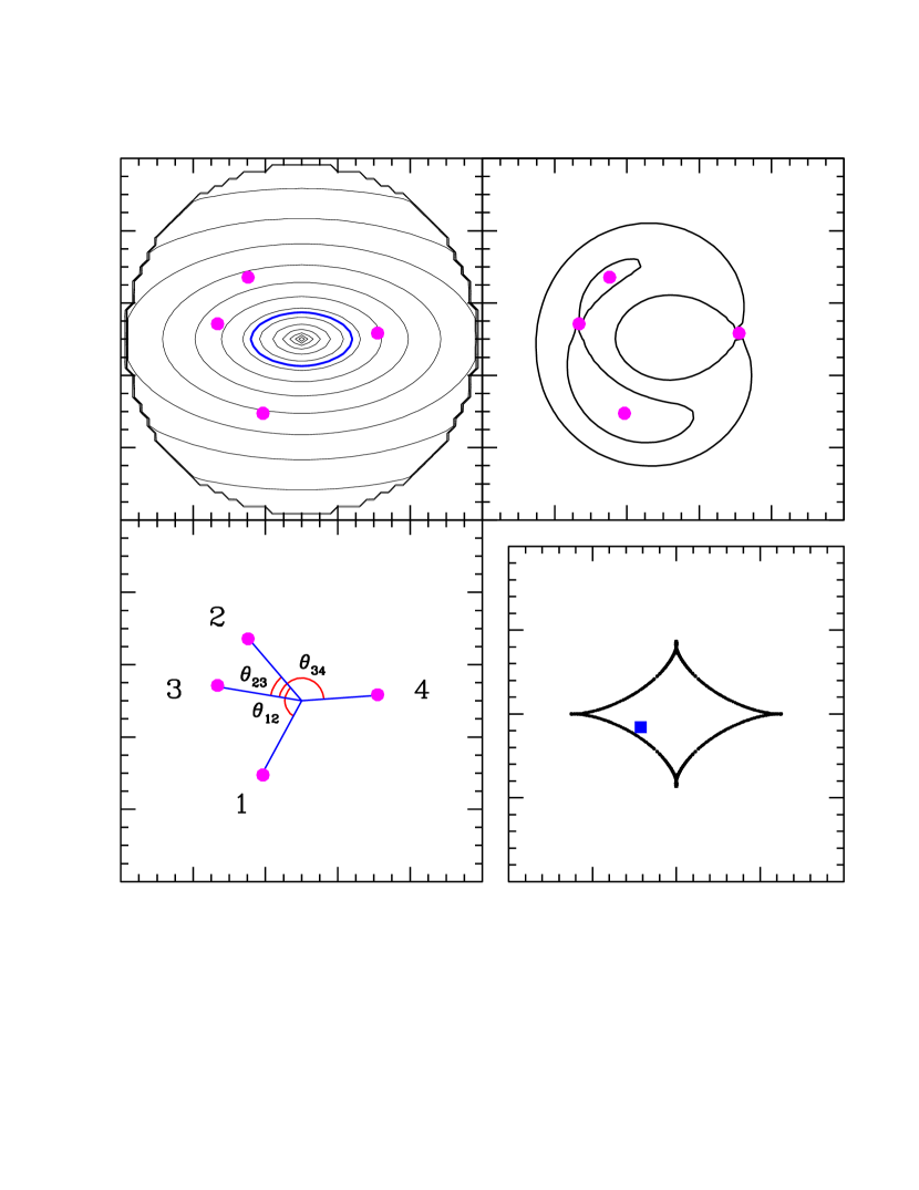
Figure 1: A representative quad from a twofold symmetric lens. Top left: An elliptical lens mass distribution, with the $\kappa=1$ contour shown as a thick blue line. Images are the magenta filled circles. Top right: Arrival time contours and images. Bottom left: Images, labeled by arrival time. The relative angles, $\theta_{12}$, $\theta_{23}$ and $\theta_{34}$ are marked. Bottom right: The diamond caustic, with the location of the source represented by a solid blue square.

A typical quad image configuration is shown in Figure 1. The images are labeled by their arrival time at the observer, 1 through 4. In most cases this ordering can be determined from the morphology of the quad, without measured time delays (Saha & Williams, 2003). Here we are interested only in the mass distribution of the lens, not its total mass (or, equivalently, its normalization), or orientation. In this case the image configuration of any quad is described uniquely by 6 parameters, which we chose to be of the polar variety, measured with respect to the lens center: three relative angles, and three distance ratios of images. The three relative angles between images are marked on the plot, $\theta_{12}$, $\theta_{34}$ and $\theta_{23}$. Angle $\theta_{12}$ is between the two minima of the arrival time surface, while $\theta_{34}$ is the angle between the saddle points. We define $\theta_{12}$ such that it encloses image 3, and $\theta_{34}$ such that it encloses image 2. Of the three angles, $\theta_{23}$ is special because the separation between images 2 and 3 gets arbitrarily small for sources approaching the diamond caustic shown in the lower right panels of Figure 1; when the source crosses the caustic these two images disappear and the quad becomes a double. Note that any linearly independent combination of the above three angles can be used, but we chose $\theta_{12}$, $\theta_{34}$ and $\theta_{23}$ because they have a simple physical meaning.

Working with only two angles, $\theta_{23}$ and a certain linear combination of $\theta_{12}$ and $\theta_{34}$, Williams et al. (2008) showed that a wide range of simple, twofold symmetric lens models generate apparently indistinguishable patterns in the two dimensional plane of these angles. Twofold symmetric means that the mass distribution, and hence the potential, is symmetric about two orthogonal axes, and ’simple’ excludes lenses with ’wavy’ isodensity shapes. The simple, twofold symmetric class of lenses includes all popular parametric lens models, such as Singular Isothermal Ellipsoids (SIE), and Singular Isothermal Elliptical Potential (SIEP), as well lenses of any density profile and ellipticity.

The present paper is an extension of Williams et al. (2008), but here we work with the full set of three angles, $\theta_{12}$, $\theta_{34}$ and $\theta_{23}$. We show that quads from all simple lens mass distributions with twofold symmetry lie on nearly the same two dimensional surface in the three dimensional space of relative angles. We call this the Fundamental Surface of Quads (FSQ). The quads from observed galaxy lenses, on the other hand, show a different behavior. As we show in Section 5, galaxy quads form a ‘cloud’ surrounding the FSQ, with typical separations from the FSQ of few to several degrees.

One can draw some interesting parallels between the FSQ we introduce here and the well studied Fundamental Plane of Ellipticals. Both lie in the three dimensional space whose axes are parameters describing the structural properties of the respective objects. In the case of quad lenses, these are the relative image angles, while in the case of ellipticals they are the effective radius, the surface brightness at the effective radius, and the central velocity dispersion. A wide class of objects belong to the Surface and the Plane with small scatter. In other words, the objects do not fill the full three dimensional space, implying that there is a tight relation between the three parameters. The existence of the Fundamental Plane is basically the consequence of the virial theorem, while the reason for the near invariance of the Fundamental Surface of Quads for a wide class of twofold symmetric lenses (but not necessarily for the observed quads) is yet to be identified.

2 The SIS+elliptical lensing model

We start by studying a simple, analytically tractable, two dimensional projected gravitational potential. It belongs to the generic family of separable potentials, $\phi(r,\theta)=r\!\cdot\!f(\theta)$, where $r$ and $\theta$ are polar coordinates in the lens plane. Properties of such potentials are discussed in Kassiola & Kovner (1993), Kochanek (1991) and Dalal (1998). For our purpose we choose

$$f(\theta)=b[1+\gamma\cos(2\theta)]$$ (1)

hence,

$$\phi=rb[1+\gamma\cos(2\theta)]$$ (2)

which is sometimes called SIS+elliptical; we will call it SISell for short. The normalization factor $b$ is the Einstein radius, and $\gamma$ is the shear parameter.

The Poisson equation, $\Delta$$\phi=2$$\kappa$, yields the projected dimensionless mass density profile,

$$\kappa=\frac{b}{2r}[1-3\gamma\cos(2\theta)].$$ (3)

Note that $\gamma$ cannot be greater than $1/3$ since otherwise $\kappa$ will have an unphysical negative value. The lens equation,

$$\vec{r_{s}}=\vec{r}-\vec{\triangledown}\phi$$ (4)

where $\vec{r_{s}}$ and $\vec{r}$ are source and image positions respectively, can be rewritten as two independent equations

$$r_{s}\cos(\theta-\theta_{s})=r-b[1+\gamma\cos(2\theta)]$$ (5)

$$r_{s}\sin(\theta-\theta_{s})=-2b\gamma\sin(2\theta)\,\,\,\Rightarrow\,\,\,-a\sin(\theta-\theta_{s})=\sin(2\theta),\,\,\,\,\,\,{a=\frac{r_{s}}{2b\gamma}}.$$ (6)

Setting the magnification $M=1/\det(A)$ , where $A$ is the Jacobian matrix of the lens equation, to infinity, i.e. $\det(A)=0$, one gets

$$\det(A)=\frac{1}{r}\left[\left(r-b\{1+\gamma\cos(2\theta)\}\right)+4b\gamma\cos\left(2\theta\right)\right]=0,$$ (7)

which yields the condition for the caustic,

$$r=b-3b\gamma\cos(2\theta).$$ (8)

Now using equation (8) in the lens equation, eq. 6, allows one to express the caustic coordinates $(r_{sc},\theta_{sc})$ in the source plane as a function of parameter $\theta$,

$$r_{sc} = b\gamma\sqrt{2[5+3\cos(4\theta)]}$$ (9)

$$\theta_{sc} = -\tan^{-1}\left(\tan^{3}\theta\right).$$ (10)

Our aim is to calculate the three relative angles, $\theta_{12}$, $\theta_{34}$ and $\theta_{23}$ for all the quads within the diamond caustic. Using eq. 6, which is independent of image distance $r$, we get the angular positions of the four images, in radians.

$$\theta_{1}=\cos^{-1}\left(\frac{1}{2}\sqrt{C+\frac{-a^{3}\cos^{3}(\theta_{s})+a\left(a^{2}-4\right)\cos(\theta_{s})+8a\cos(\theta_{s})}{4B}}-\frac{1}{4}a\cos(\theta_{s})+\frac{B}{2}\right),$$ (11)

$$\theta_{2}=\cos^{-1}\left(-\frac{1}{2}\sqrt{C-\frac{-a^{3}\cos^{3}(\theta_{s})+a\left(a^{2}-4\right)\cos(\theta_{s})+8a\cos(\theta_{s})}{4B}}-\frac{1}{4}a\cos(\theta_{s})-\frac{B}{2}\right),$$ (12)

$$\theta_{3}=\cos^{-1}\left(\frac{1}{2}\sqrt{C-\frac{-a^{3}\cos^{3}(\theta_{s})+a\left(a^{2}-4\right)\cos(\theta_{s})+8a\cos(\theta_{s})}{4B}}-\frac{1}{4}a\cos(\theta_{s})-\frac{B}{2}\right),$$ (13)

$$\theta_{4}=-\cos^{-1}\left(-\frac{1}{2}\sqrt{C+\frac{-a^{3}\cos^{3}(\theta_{s})+a\left(a^{2}-4\right)\cos(\theta_{s})+8a\cos(\theta_{s})}{4B}}-\frac{1}{4}a\cos(\theta_{s})+\frac{B}{2}\right),$$ (14)

where,

$$A=\sqrt[3]{108a^{4}\sin^{2}(2\theta_{s})+2\left(a^{2}-4\right)^{3}+12\sqrt{3}\sqrt{a^{4}\sin^{2}(2\theta_{s})\left(27a^{4}\sin^{2}(2\theta_{s})+\left(a^{2}-4\right)^{3}\right)}},$$ (15)

$$B=\sqrt{\frac{\left(a^{2}-4\right)^{2}}{62^{2/3}A}+\frac{1}{4}a^{2}\cos^{2}(\theta_{s})+\frac{1}{6}\left(4-a^{2}\right)+\frac{A}{12\sqrt[3]{2}}},$$ (16)

$$C=-\frac{\left(a^{2}-4\right)^{2}}{62^{2/3}A}+\frac{1}{2}a^{2}\cos^{2}(\theta_{s})+\frac{1}{3}\left(4-a^{2}\right)-\frac{A}{12\sqrt[3]{2}}.$$ (17)

The above equations are rather cumbersome and so preclude simple analytical expressions for the relative angles. Instead, we numerically generate random source positions within the caustic, calculate $\theta_{i}$’s using the above equations, and then compute relative angles.

The symmetry of the potential implies that it is sufficient to consider source positions only within one of the quadrants of the elliptical potential. Therefore, without any loss of generality we align the $x$-axis with the major axis of the ellipse and consider $\theta_{s}$ only from $0$ to $\pi/2$. For a given $\theta_{s}$, $r_{s}$ can vary in the range $[0$,$r_{sc}$$)$, therefore with eqs. 6 and 9 we see that $a$ runs in the range of $\Bigl{[}0,0.5\sqrt{2[5+3\cos(4\theta)]}\Bigl{)}$, which is independent of $b$ and $\gamma$, where the parameter $\theta$ is determined by the value of $\theta_{s}$ using eq. 10.

3 The Fundamental Surface of Quads

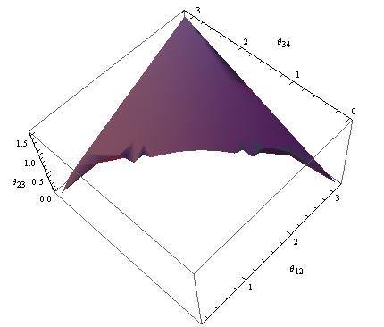
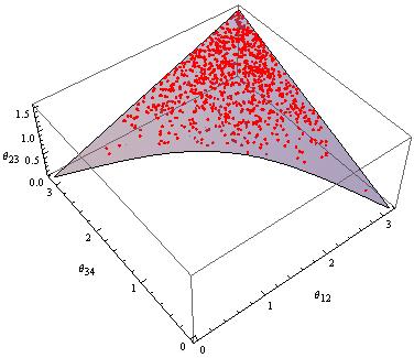
Figure 2: The three dimensional space of three image angles, $\theta_{12}$, $\theta_{23}$ and $\theta_{34}$ for the SIS+elliptical, or SISell mass distribution. (a) The surface outlined by quads whose relative image angles were calculated using eq. 11-14. (b) The fit surface to the Fundamental Surface of Quads (FSQ), eq. 3, is shown as the gray surface, while the points are quads randomly distributed within the diamond caustic in the source plane.

We use the expressions for $\theta_{i}$’s given in the previous Section to parametrically plot the relative quad angles in the three dimensional space of $\theta_{12}$, $\theta_{34}$ and $\theta_{23}$. The resulting distribution is a two dimensional surface, shown in Figure 2(a). The fact that it is a surface means that in a quad resulting from a SISell lens, two relative image angles completely determine the third.

The surface is simple with distinct properties. It has a slightly curved triangular shape with its apex at ($\theta_{12}$, $\theta_{34}$, $\theta_{23}$) = ($180^{\circ},180^{\circ},90^{\circ}$); quads at the apex have a “cross” configuration. The two edges connecting the apex to the base at $\theta_{23}=0^{\circ}$ correspond to $\theta_{12}=180^{\circ}$ and $\theta_{34}=180^{\circ}$, because in a twofold symmetric lens the latter two angles do not exceed $180^{\circ}$. Note that the base of the triangular surface that represents small values of $\theta_{23}$ and source positions close to the caustic, shows some unevenness, or jaggedness. It is unclear whether this is intrinsic to $\theta_{i}$ equations, or if it is due to the numerical noise arising from the implementation of these equations. In all what follows we ignore these small features; in particular, our fit to the surface, discussed below, smooths over this unevenness.

This surface is universal for all SISell lenses, however the meaning of universality requires some clarification. For a given source position $(\theta_{s},r_{s})$, a relative angle $\theta_{ij}$ depends on $b$ and $\gamma$, and therefore two SISell models with different $b$ and $\gamma$ give rise to two different points on the surface. However, the surface itself does not depend on $b$ and $\gamma$. This is the result of the elimination of $b$ and $\gamma$ dependence when considering all source positions within the caustic as discussed in Section 2. Therefore quads from SISell models of all shears and normalizations lie on the same invariant surface.

We would like to have an explicit functional form for the surface, as $\theta_{23}={\rm fcn}(\theta_{12},\theta_{34})$, but since the equations for individual angles, eq. 11-14, contain inverse cosines and are complicated, there is no simple expression. Instead, we calculate thousands of sets of relative angles, ($\theta_{12}$, $\theta_{34}$, $\theta_{23}$), from the expressions for the $\theta_{i}$’s (eq. 11-14) and fit these with a surface represented by a polynomial function in $\theta_{12}$ and $\theta_{34}$. The fitting was done using Matlab’s Least Absolute Errors (LAE) method. As compared to the Least Squares method, LAE is less stable and could generate more than one function. We chose LAE anyway because it is resistant to outliers, which in our case correspond to quads with small values of $\theta_{23}$, and are responsible for the jaggedness of the surface.

We determine the optimal order of the polynomial by considering the deviations, or errors, of the SISell quad points from the fit surface, quantified by the root mean square error, RMSE. A number of trials and tests revealed that a fourth order polynomial has the lowest value of RMSE, $\approx 0.00032$ radians, or $\approx 0.018^{\circ}$, for approximately 160 thousand quads. We note that using different sets of quads to obtain the fit equation resulted in slightly different values for the coefficients of the polynomial, and for some sets of quads the RMSE varied by up to a factor of two.

To test the robustness of our fit to changes in the fitting method, we also computed the best fit surface using the Least Square method, and using custom versus in-build polynomials within Matlab. Again, the resulting fit surface changed somewhat, but did not deviate substantially from the fit we present below. We conclude, therefore, that although the fit equation is not reproducible exactly, it is completely adequate for our purposes:

$$\theta_{23} = -5.792+1.783\,\theta_{12}+0.1648\,\theta_{12}^{2}-0.04591\,\theta_{12}^{3}-0.0001486\,\theta_{12}^{4}+1.784\,\theta_{34}$$

$$-0.7275\,\theta_{34}\,\theta_{12}+0.0549\,\theta_{34}\,\theta_{12}^{2}+0.01487\,\theta_{34}\,\theta_{12}^{3}+0.1643\,\theta_{34}^{2}+0.05493\,\theta_{34}^{2}\,\theta_{12}$$

$$-0.03429\,\theta_{34}^{2}\,\theta_{12}^{2}-0.04579\,\theta_{34}^{3}+0.01487\,\theta_{34}^{3}\,\theta_{12}-0.0001593\,\theta_{34}^{4}$$

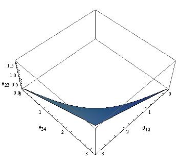
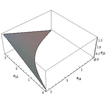
Figure 3: Two additional orientations of the Fundamental Surface of Quads.

Figure 2(b) shows the fit as the gray semi-transparent surface. The red points are SISell quads corresponding to a random distribution of source positions within the diamond caustic, on the source plane. As depicted in the Figure, a random distribution of source positions does not imply a random distribution of quads on the Fundamental Surface; quad density increases with increasing $\theta_{23}$. Two other orientations of the Fundamental Surface are shown in Figure 3.

Because the RMSE of the SISell quad distribution about the fit plane is $\hbox{\,\hbox to0.0pt{\raise 1.82986pt\hbox{$<$}\hss}\lower 2.79857pt\hbox{$\sim$}\,}0.02^{\circ}$ the differences between the two will be invisible in the full three dimensional angles space. Instead, we calculate the difference in $\theta_{23}$ of the SISell quads and the fitted surface keeping the other two angles fixed; we call this difference $\Delta\theta_{23}=\theta_{23}-\theta_{23,fit}$, where $\theta_{23,fit}$ is obtained by plugging $\theta_{12}$ and $\theta_{34}$ of a quad in to eq. 3. Figure 4 plots $\Delta\theta_{23}$ vs. $\theta_{23}$. The straight horizontal line represents the surface fit, eq. 3, while the points are the SISell quads. The wiggles in the distribution of points represents the wiggles in the SISell surface, compared to the fourth order polynomial fit. However, for all practical purposes, the differences are negligible, and eq. 3 can be taken to be a good representation of the SISell potential.

We call this surface the Fundamental Surface of Quads because, as we show in the next section, not just SISell, but most twofold symmetric models do not differ from it by more than a few degrees. This near invariance probably stems from the shape of the caustic of this class of potentials. The twofold symmetry of the lensing mass distribution implies the twofold symmetry of the diamond caustic. More specifically the diagonals of the caustic intersect at $90^{\circ}$ and all four quadrants of the caustic are identical.

4 Other two-fold symmetric potentials

In this Section we explore a wider range of simple twofold symmetric mass models, motivated by the commonly used parametric models. We calculate typical values for a total of 12 models, but show plots (see below) for only eight of these.

Two of the first four models have isothermal (SIS) radial density profiles, and the other two, de Vaucouleurs (deV) profile. Isothermal means that if mass ellipticity were zero, the projected density profile would scale as $1/r$. The de Vaucouleurs profile has projected density given by,

$$\Sigma=\Sigma_{e}\exp\left(-7.673\left[\left(r/r_{e}\right)^{1/4}-1\right]\right),$$ (19)

where $r_{e}$ is the half-mass radius, and $\Sigma_{e}$ is the projected mass density at $r_{e}$. To generate a diamond caustic the density profiles must be accompanied by either ellipticity, $e$, or external shear, $\gamma$. Ellipticity, $e$ of the mass isodensity contours is related to the axis ratio of the isodensity contours, $b/a=(1-e)/(1+e)$. The properties of the first four models are: SIS with $e=0$ and $\gamma=0.3$; deV with $e=0$ and $\gamma=0.4$; SIE with $e=0.3$ and $\gamma=0$; deV with $e=0.4$ and $\gamma=0$.

The additional eight models explore a range of power-law surface mass density profiles, $\Sigma(R)\propto R^{-\alpha}$, with $\alpha=0.4,0.7,1.3,1.6$, where isothermal slope is $\alpha=1$. The range of slopes we have chosen is considerably wider than what real lensing galaxies seem to have. Based on a well defined sample of 15 elliptical galaxy lenses, Koopmans et al. (2006) find that the typical total (dark matter and baryons) space density slope is $2.01$, or about $1$ is projection, with dispersion of $0.12$. We chose a range of slopes 5 times wider than that because we would like to demonstrate the robustness of the FSQ to changes in the lens model parameters. Each of these four density profile slope models were given $e=0.25$, or $\gamma=0.25$. These values are somewhat on the high side of the typical values for ellipticity and shear encountered in modeling observed quads.

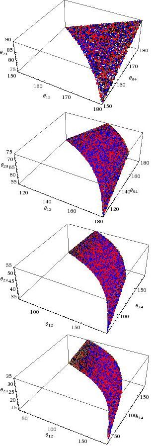
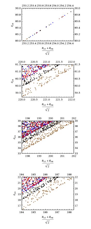
Figure 5: Simple twofold symmetric lens mass distributions define a nearly invariant Fundamental Surface of Quads. Quads from four mass models are shown: SIS with $e=0$ and $\gamma=0.3$ (red); deV with $e=0$ and $\gamma=0.4$ (blue); SIE with $e=0.3$ and $\gamma=0$ (black); deV with $e=0.4$ and $\gamma=0$ (brown). On the left we show the 3D space of relative angles sliced into four segments divided by $\theta_{23}=35^{\circ},55^{\circ},75^{\circ}$. The fact that the points of different lens potentials are hard to tell apart demonstrates the near invariance of the FSQ. To make the deviations visible, on the right we fold and project a small angle range of the surface; see Section 4 for details.

Each mass model generates a two dimensional surface in the three dimensional space of relative angles. All surfaces coincide at the apex, where $(\theta_{12},\theta_{34},\theta_{23})=(180^{\circ},180^{\circ},90^{\circ})$, since all twofold symmetric models can produce a perfect cross configuration (though the distance ratios of images will differ). At other locations the surfaces deviate from each other somewhat, and from the one defined by SISell; largest deviations are seen at small $\theta_{23}$ values, i.e. towards the base of the triangular surface. However, even at the widest separation, the surfaces differ by only a few degrees. The left panel of Figure 5 shows that these differences are hard to discern in the full three dimensional angles space, even if the surface is split up into four pieces for easier visualization. To make the deviations visible, in the right panel of Figure 5 we fold the surface along the vertical mid-line, and show only a narrow range of angles, a few degrees in each case. In this zoom, the deviations are seen to be a few degrees.

Another way to show deviations is to use $\Delta\theta_{23}$ introduced in the previous Section; see Figures 6 and 7. As before the horizontal line at $\Delta\theta_{23}=0$ represents the Fundamental Surface of Quads, given by the fit eq. 3, and the points are quads from lens mass models. In Figure 6 the isothermal models and the de Vaucouleurs models are shown in the left and right panels, respectively. The top row shows the models with external shear, $\gamma$, while the bottom rows represent elliptical mass distributions. In Figure 7 four mass models with power-law density profiles are shown.

To quantify the effect of shear or ellipticity on any given mass model, we quote the average distance ratio $<d_{4}/d_{1}>$, where $d_{1}$ and $d_{4}$ are the distances of the first and fourth arriving images from the lens center, and the average is over quads randomly populating the inside of the diamond caustic. A given lens mass distribution produces quads with a range of image distance ratios, but in general image 1 tends to be farthest from the lens center, while image 4 tends to be closest. For the 12 models, $<d_{4}/d_{1}>$ is between 0.5 and 0.9. For the sample of 40 observed quads (Section 5) $<d_{4}/d_{1}>\sim 0.68$. i.e. typically smaller than in our models. As will be discussed in the next Section many of the observed quads are the result of mass distributions that are more involved than two-fold symmetric lenses; most require an external shear in addition to and elliptical lens, while some require substructure. The presence of these would tend to reduce the $d_{4}/d_{1}$ ratio.

Table 1 summarizes the results of the 12 models. In general, larger ellipticities or larger $\gamma$ result in larger deviations from the FSQ. Because the maximum deviations from FSQ differ between models from a fraction of a degree to a few degrees, the range on the vertical axes range are different in the top and bottom panels of Figures 6 and 7. As opposed to the quad distributions generated by the elliptical mass models, the ones from models with external shear are much closer to the FSQ, and appear more similar to that of the SISell model (unless the surface mass density is very shallow, as in the bottom right panel of Figure 7). When viewed in 3D, the surfaces containing quads from the elliptical lens models sag below the FSQ, but even for the bottom right panel of Figure 6 the deviations in $\theta_{23}$ are $<4^{\circ}$, for $e=0.4$, and de Vaucoulers profile. Here the images are formed where the projected density $\Sigma(R)\propto R^{-2}$, or $\rho(r)\propto r^{-3}$ in three dimensions. Given observed lenses, this is a rather extreme combination of ellipticity and $\Sigma(R)$. Ellipticity of $e=0.4$ corresponds to the axis ratio $b/a=0.43$, or an E5.7 if it were an optical elliptical galaxy. Steep density profiles also appear to result in larger deviations from the FSQ; see Table 1. Real galaxy lenses rarely, if at all, have such steep profiles at the location of quad images. For $e=0.25$, and $\Sigma(R)\propto R^{-0.4...-1.6}$ (top right and bottom left panels of Figure 7), the deviations from FSQ are a degree at most.

We note that for very large ellipticities or shears (not considered here) the two opposite cusps of the diamond caustic protrude outside of the oval caustic producing so-called naked cusps, which do not produce quads. The corresponding surfaces of relative angles look similar to the ones without the naked cusps, except that the portions at the bottom corners of the surface are devoid of quads.

5 Observed Quads

In this Section we illustrate one of the practical uses of the Fundamental Surface of Quads (FSQ).

Galaxy lens systems can be approximately divided into three categories, depending on whether the lens mass model is (a) an elliptical mass distribution or a circularly symmetric mass distribution with an external shear, (b) an elliptical mass distribution plus some external shear, or (c) a more complicated mass distribution, possibly with additional lens galaxies or substructure mass clumps. A survey of the literature indicates that only a handful of systems belong to (a). A model-free way to come to that conclusion is to look at the quads in the 3D angles space.

We have assembled a sample of 40 galaxy-lens quads. The sample was collected from all available sources, and is therefore heterogeneous. Where possible, the astrometry, including the positional uncertainties on the images and the lensing galaxy was taken from the CASTLeS web-site (Kochanek et al., 2008); otherwise from individual papers. In the latter case, systems listed in Table The Fundamental Surface of Quad Lenses have a footnote with a reference; a lens system with no reference means that its data were obtained entirely from CASTLeS. The image arrival time was determined from the morphology of the lens (Saha & Williams, 2003), and the relative angles were calculated. These are listed in Table The Fundamental Surface of Quad Lenses, in columns labeled $\theta_{12}$, $\theta_{34}$ and $\theta_{23}$.

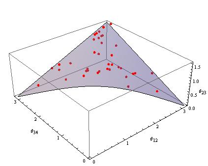
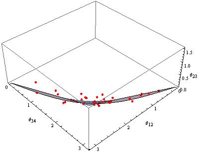
Figure 8: The Fundamental Surface of Quads fit equation (shaded region) and the forty observed galaxy quads (red dots). Two orientations are shown; in the second one the deviation of the observed quads from the Plane are clearly visible.

In Figure 8 we show two orientations of the 3D angles space with the FSQ and the 40 quads. For clarity, we do not show errors in this plot. The main conclusion is that most observed quads lie more than a few degrees away from the FSQ; 12 are within $\pm 2^{\circ}$, so most cannot be modeled adequately with an elliptical lens, or a circularly symmetric lenses with external shear.

Next, we incorporate errors into the analysis. Even though the astrometric measurement errors of images and galaxy lens center are largely independent of each other, a shift in the lens center translates into correlated relative angle errors. To account for this we calculate the errors as follows. We assume that the $x,~{}y$ positional errors of each of the four images and the lens center are normally distributed, with $\sigma_{x}$ and $\sigma_{y}$ taken from the literature. We then draw thousands of independent image and lens center positions, and for each generated lens system calculate relative angles $\theta_{12}$, $\theta_{34}$ and $\theta_{23}$. The thousands of generated quads per lens system then give us the error distribution for each of the three relative angles. We calculate the mean and the rms of these distributions, and list them in columns labeled $\theta_{ij,errors}$ in Table The Fundamental Surface of Quad Lenses. Note that the average of these distributions need not be the same as $\theta_{ij}$, however, the differences tend to be small, generally $<0.1^{\circ}$.

We quantify the deviation of the quads from the FSQ as in earlier Sections, by calculating $\Delta\theta_{23}$. The error in $\Delta\theta_{23}$, listed as $\Delta\theta_{23,errors}$ is calculated similarly to what was described above, using thousands of quads generated based on astrometric uncertainty.

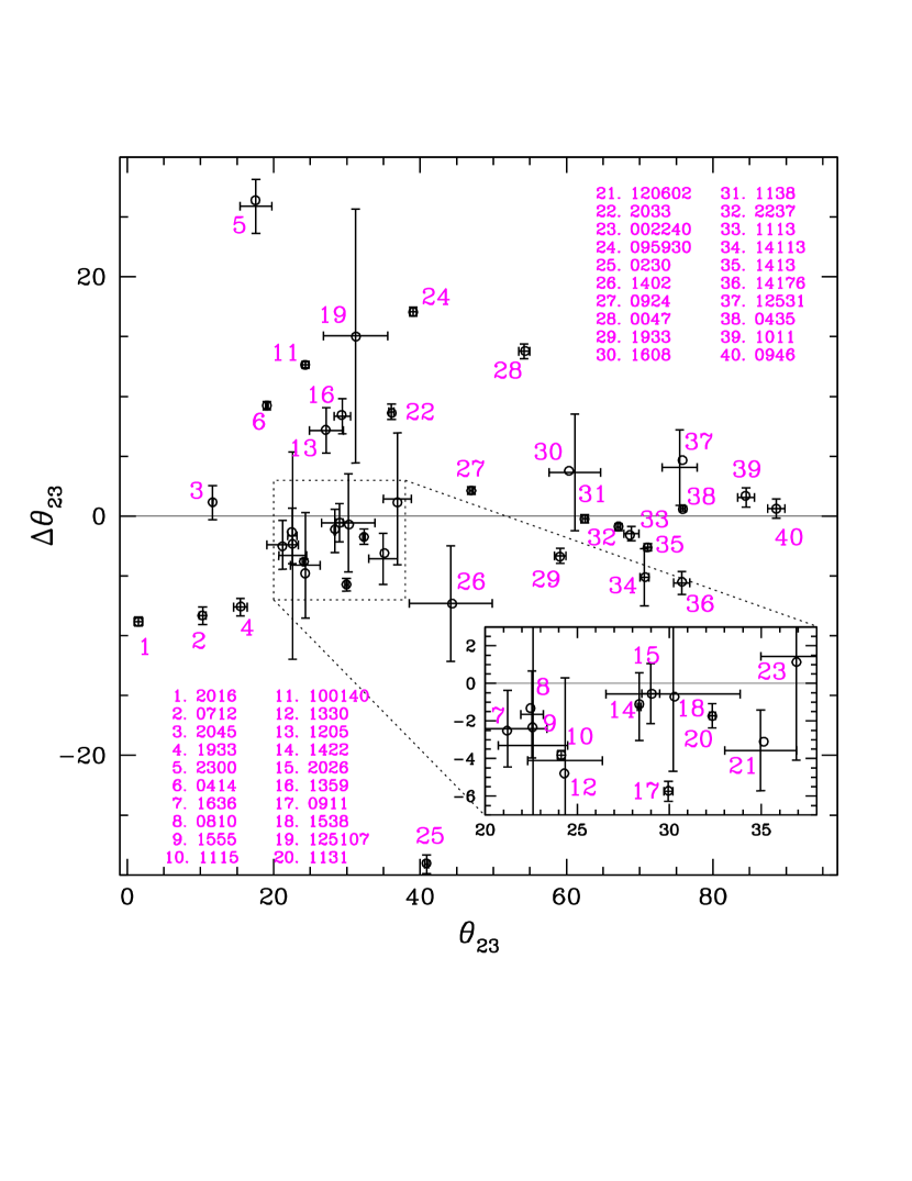
Figure 9: Deviations, $\Delta\theta_{23}$, of the observed quads from the FSQ. The horizontal axis is the observed $\theta_{23}$. The empty circles represent the observed relative angles and their deviations from the FSQ. The error bars are calculated as explained in Section 5. The horizontal and vertical axes values are given in Table 1.

Figure 9 shows the distribution of the 40 quads in the $\theta_{23}$ vs. $\Delta\theta_{23}$ plane. Within errorbars, only 10 systems are consistent with FSQ. Several of these have published parametric modeling, and are, in fact, well represented by two-fold symmetric mass distributions. For example, B2045+265 is successfully modeled by Fassnacht et al. (1999) using SISell potential, eq. 2. SDSS J002240 is modeled by Allam et al. (2007) with Singular Isothermal Ellipsoid (SIE) using gravlens software of Keeton (2001). The same software was used by Grillo et al. (2010) to fit the positions (not the flux ratios) of SDSS J1538 with three types of twofold symmetric models: de Vaucoulers, SIE and a power law density profile.

On the other hand, some of the lenses which lie away from the FSQ are known to require external shear in addition to elliptical lens. PG 1115 where the lensing galaxy is a member of a galaxy group is inconsistent with FSQ; its $|\Delta\theta_{23}|\sim 4^{\circ}$. RXJ 0911+0551 has a cluster next to it (Burud et al., 1998), so the lens model requires an external shear in addition to an elliptical galaxy lens; its $|\Delta\theta_{23}|\sim 6^{\circ}$. For LSD Q0047-2808, Koopmans & Treu (2003) state that SIE+shear does not fit the image positions well (but sufficient for the determination of the Einstein ring radius); it has $|\Delta\theta_{23}|\sim 14^{\circ}$. Lenses with known secondary galaxies also lie far from the FSQ. HE 0230-2130 has a secondary lensing galaxy (Wisotzki et al., 1999) very close to the images, and so its $|\Delta\theta_{23}|\sim 30^{\circ}$. B1608 has a complicated galaxy merger as a lens, and its $|\Delta\theta_{23}|\sim 5^{\circ}$, and so it is inconsistent with the FSQ.

A few caveats are in order. If a quad does not lie within a couple of degrees of the Fundamental Surface of Quads (i.e. the range defined by the various density profile and ellipticity models, such as the ones in Figure 5, 6 and 7), it cannot be modeled by a twofold symmetric lens. However, the opposite need not be true. If a quad lies on the FSQ does that immediately imply that it can be modeled by a twofold symmetric lens, regardless of its image distance ratios? This question will be addressed in a future study. We also note that even if a quad does belong to the locus of twofold symmetric lens in the full 6D space of image position properties, it does not mean that other types of lens models cannot fit it. Reconstruction of the lens mass reconstruction from single quads is a highly underconstrained problem, so the solution is not unique, and many mass models can reproduce the image positions exactly (Saha & Williams, 2004).

6 Conclusions and Future Work

In this paper we present a model-free way of making inferences about the lensing mass distribution given its quad image positions. The latter are represented by three relative angles that describe the distribution of images around the lens center. We show that in the three dimensional space of these angles, quads generated by SIS+elliptical mass distribution belong to an invariant two dimensional surface, regardless of the shear parameter $\gamma$, and normalization $b$. Furthermore, quads from a wider class of lenses with twofold symmetry outline almost the same surface, making the surface a near invariant descriptor of twofold symmetric mass distributions. Because of that property we call the two dimensional surface the Fundamental Surface of Quads (FSQ).

The existence of FSQ allows one to characterize galaxies and clusters based on the quads they generate. To aid in that, we provide a fitting formula for the FSQ based on the SIS+elliptical lensing potential. If a quad does not lie within a couple of degrees of the FSQ (i.e. the range defined by the various density profile and ellipticity models, such as the ones in Figure 5, 6, and 7), the mass distribution is not twofold symmetric. This method of determining if a lens can be fit with a twofold symmetric lens is superior to answering this question using parametric modeling. The latter fits quads with a finite set of models, while our method addresses all twofold symmetric models irrespective of the specific parametric form.

However, the main importance of the FSQ is not in ascertaining if the lens mass distribution is twofold symmetric or not, but in the following aspects, which we will investigate in the forthcoming papers. First, the near invariance of FSQ provides a new framework for studying quads, and strong lensing theory in general. We remind the reader that it is still not understood why a wide class of twofold symmetric lenses form such a tight, near invariant distribution in the space of relative angles. Second, as already shown in Williams et al. (2008), the relative angles present a promising way of investigating realistic mass distributions, and specifically, differentiating substructured lenses from smooth non-twofold symmetric ones. Finally, the full set of quad image properties lives in the six dimensional space that includes image distance ratios. An investigation of this space is yet to be undertaken.

Table 1: Summary of lens mass models

Lens Mass Model	$<d_{4}/d_{1}>$	rms $(0^{\circ}\!\!-\!90^{\circ})$	rms $(0^{\circ}\!\!-\!30^{\circ})$	rms $(30^{\circ}\!\!-\!60^{\circ}$)	rms $(60^{\circ}\!\!-\!90^{\circ})$
SIS with $\gamma=0.3$ ($\Sigma\propto R^{-1}$)	0.74	0.025	0.042	0.021	0.016
SIE with $e=0.3$ ($\Sigma\propto R^{-1}$)	0.78	0.601	0.877	0.600	0.223
deV with $\gamma=0.4$ ($\Sigma\propto R^{-3}$)	0.79	0.0526	0.0849	0.0487	0.0224
deV with $e=0.4$ ($\Sigma\propto R^{-2}$)	0.79	1.431	1.948	1.457	0.541
$\Sigma(R)\propto R^{\,-0.4}$ with $e=0.25$	0.69	0.148	0.211	0.153	0.0676
$\Sigma(R)\propto R^{\,-0.7}$ with $e=0.25$	0.76	0.322	0.475	0.323	0.125
$\Sigma(R)\propto R^{\,-1.3}$ with $e=0.25$	0.91	0.547	0.802	0.548	0.210
$\Sigma(R)\propto R^{\,-1.6}$ with $e=0.25$	0.91	0.565	0.810	0.564	0.222
$\Sigma(R)\propto R^{\,-0.4}$ with $\gamma=0.25$	0.51	0.356	0.603	0.347	0.100
$\Sigma(R)\propto R^{\,-0.7}$ with $\gamma=0.25$	0.85	0.0432	0.0716	0.0403	0.0101
$\Sigma(R)\propto R^{\,-1.3}$ with $\gamma=0.25$	0.82	0.0592	0.0816	0.0583	0.413
$\Sigma(R)\propto R^{\,-1.6}$ with $\gamma=0.25$	0.85	0.0342	0.0591	0.0282	0.0159

The first four lens models are shown in Figure 6, and a subset of the other eight are in Figure 7. For the first four the slope of the projected surface mass density, $\Sigma(R)$, at the location of the images is indicated in parentheses. For de Vaucouleurs models the slope of the density profile changes with radius, so the value of the slope is a typical value for the radii where the images form. The other eight density profiles are power-laws in radius. The quantity $<d_{4}/d_{1}>$ is the average ratio of the distance of the 4th and 1st arriving images. In the third column, rms $(0^{\circ}\!\!-\!90^{\circ})$ is the rms value of $\Delta\theta_{23}$ for all the images, i.e. those with the full range of $\theta_{23}$, or $0^{\circ}\!\!-\!90^{\circ}$. The last three columns show rms values for three subsets of images, divided by their $\theta_{23}$ values. All rms are quoted in degrees.

Table 2: Relative angles

N	Lens name	$\theta_{12}$	$\theta_{12,{\rm{errors}}}$	$\theta_{34}$	$\theta_{34,{\rm{errors}}}$	$\theta_{23}$	$\theta_{23,{\rm{errors}}}$	$\Delta\theta_{23}$	$\Delta\theta_{23,{\rm{errors}}}$
1	MG 2016+112	150.8	150.7 $\pm$ 0.4	91.4	91.3 $\pm$ 0.6	1.5	1.5 $\pm$ 0.6	-8.8	-8.8 $\pm$ 0.4
2	B 0712+472	79.8	79.8 $\pm$ 0.3	163.2	163.3 $\pm$ 0.7	10.2	10.3 $\pm$ 0.4	-8.3	-8.3 $\pm$ 0.7
3	B 2045+265	34.9	34.9 $\pm$ 0.1	175.2	175.2 $\pm$ 1.0	11.7	11.7 $\pm$ 0.1	1.2	1.1 $\pm$ 1.4
4	B 1933+503 lobe	155.5	155.5 $\pm$ 0.7	101.7	101.7 $\pm$ 0.9	15.5	15.5 $\pm$ 0.9	-7.6	-7.6 $\pm$ 0.7
5	SLACS J2300+002	160.8	161.2 $\pm$ 2.0	38.5	38.5 $\pm$ 2.0	17.5	17.6 $\pm$ 2.2	26.4	25.9 $\pm$ 2.3
6	MG 0414+0534	101.5	101.5 $\pm$ 0.3	144.1	144.1 $\pm$ 0.3	19.1	19.1 $\pm$ 0.2	9.2	9.2 $\pm$ 0.3
7	SLACS J1636+470	128.0	127.9 $\pm$ 1.8	136.9	136.9 $\pm$ 2.5	21.2	21.2 $\pm$ 2.1	-2.5	-2.4 $\pm$ 2.0
8	HS 0810+2554	111.3	111.5 $\pm$ 1.1	150.1	150.4 $\pm$ 2.3	22.5	22.5 $\pm$ 0.6	-1.3	-1.7 $\pm$ 2.3
9	B 1555+375	114.0	113.1 $\pm$ 5.9	149.3	150.6 $\pm$10.7	22.6	22.6 $\pm$ 1.9	-2.3	-3.3 $\pm$ 8.7
10	PG 1115+080	141.9	141.9 $\pm$ 0.3	127.5	127.5 $\pm$ 0.4	24.1	24.1 $\pm$ 0.2	-3.8	-3.8 $\pm$ 0.3
11	J 100140.12+020	120.4	120.4 $\pm$ 0.1	131.3	131.3 $\pm$ 0.5	24.3	24.3 $\pm$ 0.4	12.6	12.7 $\pm$ 0.2
12	SDSS J1330+1810	115.6	115.7 $\pm$ 3.2	152.2	151.5 $\pm$ 4.8	24.3	24.3 $\pm$ 2.0	-4.8	-4.1 $\pm$ 4.4
13	SLACS J1205+491	159.1	159.3 $\pm$ 1.9	90.4	90.3 $\pm$ 2.1	27.1	27.2 $\pm$ 2.3	7.2	7.2 $\pm$ 1.9
14	B 1422+231	74.8	74.8 $\pm$ 0.3	173.8	174.0 $\pm$ 1.4	28.4	28.4 $\pm$ 0.1	-1.1	-1.2 $\pm$ 1.8
15	WFI 2026-4536	154.1	154.1 $\pm$ 1.8	113.6	113.5 $\pm$ 1.3	29.1	29.0 $\pm$ 0.5	-0.5	-0.5 $\pm$ 1.6
16	CLASS B1359+154	135.9	135.8 $\pm$ 1.2	125.8	126.1 $\pm$ 3.2	29.3	29.4 $\pm$ 1.1	8.4	8.3 $\pm$ 1.5
17	RXJ 0911+0551	180.7	180.7 $\pm$ 0.5	69.6	69.7 $\pm$ 0.4	29.9	29.9 $\pm$ 0.2	-5.7	-5.7 $\pm$ 0.5
18	SDSS J1538+5817	152.7	152.7 $\pm$ 4.0	117.7	117.3 $\pm$ 4.0	30.3	30.2 $\pm$ 3.6	-0.7	-0.6 $\pm$ 4.1
19	SDSS J125107	158.8	158.1 $\pm$ 9.9	85.2	86.4 $\pm$ 8.8	31.3	31.2 $\pm$ 4.4	15.0	15.1 $\pm$10.6
20	RXJ 1131-1231	66.0	66.0 $\pm$ 0.2	180.9	180.8 $\pm$ 0.5	32.3	32.3 $\pm$ 0.2	-1.8	-1.7 $\pm$ 0.6
21	SDSS J120602.09	96.0	95.9 $\pm$ 2.2	171.6	171.9 $\pm$ 2.1	35.1	35.0 $\pm$ 2.0	-3.1	-3.6 $\pm$ 2.1
22	WFI 2033-4723	140.6	140.5 $\pm$ 0.6	128.5	128.5 $\pm$ 0.7	36.1	36.1 $\pm$ 0.3	8.6	8.7 $\pm$ 0.6
23	SDSS J002240	77.9	78.3 $\pm$ 1.8	177.5	177.1 $\pm$ 4.4	36.9	36.9 $\pm$ 1.9	1.1	1.4 $\pm$ 5.5
24	J 095930.94+023	141.2	141.2 $\pm$ 0.4	120.9	121.0 $\pm$ 0.5	39.0	39.1 $\pm$ 0.5	17.0	17.1 $\pm$ 0.4
25	HE 0230-2130	127.2	127.2 $\pm$ 0.3	186.7	186.8 $\pm$ 0.9	40.9	40.9 $\pm$ 0.3	-29.0	-29.1 $\pm$ 0.8
26	SDSS 1402+6321	142.6	142.7 $\pm$ 6.1	156.1	155.7 $\pm$ 6.8	44.4	44.2 $\pm$ 5.6	-7.3	-7.3 $\pm$ 4.8
27	SDSS 0924+0219	153.6	153.6 $\pm$ 0.4	135.9	135.9 $\pm$ 0.5	47.0	47.0 $\pm$ 0.3	2.1	2.1 $\pm$ 0.3
28	LSD Q0047-2808	130.9	130.8 $\pm$ 0.7	152.8	152.7 $\pm$ 0.8	54.3	54.2 $\pm$ 0.8	13.8	13.8 $\pm$ 0.6
29	B 1933+503 core	169.1	169.1 $\pm$ 0.8	142.8	142.8 $\pm$ 0.8	59.1	59.1 $\pm$ 0.8	-3.4	-3.3 $\pm$ 0.6
30	B 1608+656	97.9	99.2 $\pm$ 5.9	186.7	187.2 $\pm$ 4.9	60.3	61.1 $\pm$ 3.5	3.8	3.7 $\pm$ 4.9
31	SDSS 1138+0314	153.1	153.1 $\pm$ 0.5	161.1	161.1 $\pm$ 0.6	62.5	62.5 $\pm$ 0.3	-0.2	-0.2 $\pm$ 0.4
32	Q 2237+0305	146.3	146.3 $\pm$ 0.4	173.4	173.5 $\pm$ 0.6	67.1	67.1 $\pm$ 0.3	-0.9	-0.9 $\pm$ 0.3
33	HE 1113-0641	154.4	154.6 $\pm$ 1.2	170.3	170.3 $\pm$ 1.2	68.6	68.9 $\pm$ 1.0	-1.6	-1.5 $\pm$ 0.6
34	HST 14113+5211	163.2	163.2 $\pm$ 0.6	171.0	171.0 $\pm$ 3.8	70.7	70.6 $\pm$ 0.6	-5.1	-5.1 $\pm$ 2.4
35	H 1413+117	160.3	160.3 $\pm$ 0.6	170.3	170.4 $\pm$ 0.7	71.1	71.1 $\pm$ 0.4	-2.6	-2.6 $\pm$ 0.3
36	HST 14176+5226	163.1	163.1 $\pm$ 0.5	179.5	179.6 $\pm$ 1.6	75.8	75.7 $\pm$ 1.1	-5.5	-5.6 $\pm$ 1.0
37	HST 12531-2914	149.9	149.6 $\pm$ 2.2	175.0	175.5 $\pm$ 4.4	75.8	75.4 $\pm$ 2.4	4.7	4.1 $\pm$ 3.2
38	HE 0435-1223	155.1	155.2 $\pm$ 0.3	176.8	176.7 $\pm$ 0.3	75.9	75.9 $\pm$ 0.3	0.6	0.6 $\pm$ 0.2
39	SDSS 1011+0143	169.7	169.9 $\pm$ 0.9	176.4	176.6 $\pm$ 1.5	84.4	84.5 $\pm$ 1.2	1.7	1.6 $\pm$ 0.8
40	SLACS J0946+100	182.9	182.9 $\pm$ 0.9	172.8	172.7 $\pm$ 1.1	88.6	88.6 $\pm$ 1.2	0.6	0.6 $\pm$ 0.8

References. — MG 2016+112 (Nair & Garrett, 1997; Lawrence et al., 1984), B2045+265 (Fassnacht et al., 1999), B 1933+503 (Nair, 1998), SLACS J2300+002, SLACS J1636+470, SLACS J1205+491 (Ferreras et al., 2008), SDSS J125107 (Kayo et al., 2007), SDSS J1330+1810 (Oguri et al., 2008), J 100140.12+020 (Jackson, 2008), SDSS J1538+5817 (Grillo et al., 2010), SDSS J002240 (Allam et al., 2007), SDSS J120602.09 (Lin et al., 2009), J 095930.94+023 (Jackson, 2008), SDSS 1402+6321 (Bolton et al., 2005), LSD Q0047-2808 (Koopmans & Treu, 2003), HE 1113-0641 (Blackburne et al., 2008), SLACS J0946+100 (outer ring) (Gavazzi et al., 2008)

Figure 4: Deviations of the SISell quads from the best fit 4th degree polynomial presented in equation 3. The vertical axis shows the deviations of the quads’ $\theta_{23}$ from the prediction of equation 3. The quads used to compute the best fit were obtained using analytical equations for angles $\theta_{1}$, $\theta_{2}$, $\theta_{3}$ and $\theta_{4}$ presented in Section 2, while the quads in this Figure were generated using a ray tracing code. The difference between the two is small.

Figure 6: The deviations of the quads of four mass distributions from the predictions of the 4th degree polynomial fit, equation 3. The four mass distributions are the same as the ones shown in Figure 5 Top left: Circularly symmetric SIS surface mass density with external shear $\gamma=0.3$; Top right: Circularly symmetric de Vaucoulers with external shear $\gamma=0.4$; Bottom left: Elliptical SIE with ellipticity 0.3; Bottom left: Elliptical de Vaucoulers with ellipticity 0.4. The average value of the distance ratio of the fourth to first arriving image, $<d_{4}/d_{1}>$, is shown in each panel. This aids in visualizing the meaning of $\gamma$ and $e$ value. Note that the vertical axes have different ranges in the top and bottom panels.

Figure 7: Same as Figure 6, but for a different set of lens mass models. Top left: Circularly symmetric surface mass density, $\Sigma(R)\propto R^{\,-1.6}$ with external shear $\gamma=0.25$; Top right: Elliptical $\Sigma(R)\propto R^{\,-0.4}$ with ellipticity 0.25; Bottom left: Elliptical $\Sigma(R)\propto R^{\,-1.6}$ with ellipticity 0.25; Bottom left: Circularly symmetric $\Sigma(R)\propto R^{\,-0.4}$ with external shear $\gamma=0.25$.

References

- Allam et al. (2007) Allam, S. S., Tucker, D. L., Lin, H., Diehl, H. T., Annis, J., Buckley-Geer, E. J., Frieman, J. A. 2007, ApJ, 662, L51
- Blackburne et al. (2008) Blackburne, J.A., Wisotzki, L. Schechter, P.L. 2008, AJ, 135, 374
- Bolton et al. (2005) Bolton, A.S., Burles, S., Koopmans, L.V.E., Treu, T., Moustakas, L.A. 2005, ApJ, 624, L21
- Burud et al. (1998) Burud, I. et al. 1998, ApJ, 501, L5
- Dalal (1998) Dalal, N. 1998, ApJ, 509, L13
- Fassnacht et al. (1999) Fassnacht, C. D. et al. 1999, AJ, 117, 658
- Ferreras et al. (2008) Ferreras, I., Saha, P., Burles, S. 2008, MNRAS, 383, 857
- Gavazzi et al. (2008) Gavazzi, R., Treu, T., Koopmans, L. V. E., Bolton, A. S., Moustakas, L. A., Burles, S., Marshall, P. J. 2008, ApJ, 677, 1046
- Grillo et al. (2010) Grillo, C., Eichner, T., Seitz, S., Bender, R., Lombardi, M., Gobat, R., Bauer, A. 2010, ApJ, 710, 372
- Jackson (2008) Jackson, N. 2008, MNRAS, 389, 1311
- Kassiola & Kovner (1993) Kassiola, A. & Kovner, I. 1993, ApJ, 417, 450
- Kayo et al. (2007) Kayo, I. et al. 2007, AJ, 134, 1515
- Keeton (2001) Keeton, C. R. 2001, eprint arXiv:astro-ph/0102341
- Kochanek (1991) Kochanek, C.S. 1991, ApJ 373, 354
- Kochanek et al. (2008) Kochanek, C.S., Falco, E.E., Impey, C., Lehar, J., McLeod, B. & Rix, H.-W. CASTLeS website, http://cfa-www.harvard.edu/glensdata/
- Koopmans et al. (2009) Koopmans, L. V. E. et al. 2009, ApJ, 703, L51
- Koopmans & Treu (2003) Koopmans, L. V. E. & Treu, T. 2003, ApJ, 583, 606
- Koopmans et al. (2006) Koopmans, L. V. E., Treu T., Bolton A. S., Burles, S., Moustakas L. A. 2006, ApJ, 649, 599
- Lawrence et al. (1984) Lawrence, C. R., Schneider, D. P., Schmidet, M., Bennett, C. L., Hewitt, J. N., Burke, B. F., Turner, E. L., Gunn, J. E. 1984, Science, 223, 46
- Lin et al. (2009) Lin, Huan, et al. 2009, ApJ, 699, 1242
- Nair (1998) Nair, S. 1998, MNRAS, 301, 315
- Nair & Garrett (1997) Nair, S., Garrett, M.A. 1997, MNRAS, 284, 58
- Oguri et al. (2008) Oguri, M., Inada, N., Blackburne, J.A., Shin, M.-S., Kayo, I., Strauss, M.A., Schneider, D.P., York, D.G. 2008, MNRAS, 391, 1973
- Saha & Williams (2004) Saha, P. & Williams, L.L.R. 2003, AJ, 127, 2604
- Saha & Williams (2003) Saha, P. & Williams, L.L.R. 2003, AJ, 125, 2769
- Williams et al. (2008) Williams, L.L.R., Foley, P., Farnsworth, D., & Belter, J. 2008. ApJ, 685, 725
- Wisotzki et al. (1999) Wisotzki, L., Christlieb, N., Liu, M. C., Maza, J., Morgan, N. D., Schechter, P. L. 1999, A&A, 48, L41
- Witt & Mao (1997) Witt, H. J., & Mao, S. 1997, MNRAS, 291, 211