Kinematic entanglement degradation of fermionic cavity modes

Abstract

We analyse the entanglement and the nonlocality of a $(1+1)$-dimensional massless Dirac field confined to a cavity on a worldtube that consists of inertial and uniformly accelerated segments, for small accelerations but arbitrarily long travel times. The correlations between the accelerated field modes and the modes in an inertial reference cavity are periodic in the durations of the individual trajectory segments, and degradation of the correlations can be entirely avoided by fine-tuning the individual or relative durations of the segments. Analytic results for selected trajectories are presented. Differences from the corresponding bosonic correlations are identified and extensions to massive fermions are discussed.

I Introduction

One of the fundamental problems in the emerging field of relativistic quantum information is the degradation of correlations caused by accelerated motion. Studies of uniform acceleration in Minkowski spacetime (see alsingmilburn03 ; fuentesschullermann05 ; alsingfuentesschullermanntessier06 ; bruschiloukomartinmartinezdraganfuentes10 ; martinmartinezfuentes11 ; friiskoehlermartinmartinezbertlmann11 for a small selection and MartinMartinez:2011mw for a recent review) have revealed significant differences in the degradation that occurs for bosonic and fermionic fields. There are in particular clear qualitative differences in the bosonic versus fermionic particle-antiparticle entanglement swapping martinmartinezfuentes11 and in the infinite acceleration residual entanglement and nonlocality friiskoehlermartinmartinezbertlmann11 .

The analyses of uniform acceleration mentioned above involve two ingredients that make it difficult to compare the theoretical predictions to experimentally realisable situations. The first is that while the uniformly-accelerated observers are considered to be pointlike and perfectly localised on a trajectory of prescribed acceleration, the field excitations are nevertheless usually treated as delocalised field modes of plane wave type, normalised in the sense of Dirac rather than Kronecker deltas. This may seem a technicality, perhaps remediable by use of appropriate wave packets bruschiloukomartinmartinezdraganfuentes10 , but at present it appears unexplored how localised observers would in practice perform measurements to probe the correlations in the delocalised states.

The second concern lies in the time evolution of the correlations. An inertial trajectory in Minkowski space is stationary, in the sense that it is the integral curve of a Minkowski time translation Killing vector. A uniformly-accelerated trajectory is also stationary, in the sense that it is the integral curve of a boost Killing vector. However, the combined system of the two trajectories is not stationary, as the two Killing vectors do not commute. For example, in the $(1+1)$-dimensional setting there is a unique moment at which the two trajectories are parallel, and the trajectories may or may not intersect depending on their relative spatial location. Yet the analyses mentioned above regard the correlations between observers on the two trajectories as stationary and the relative location of the trajectories as irrelevant, observing just that the spacetime has a quadrant causally disconnected from the uniformly-accelerated worldline and noting that the field modes confined in this quadrant are inaccessible to the accelerated observer. While the acceleration horizon that is responsible for this inaccessibility may be seen as the basis of the Unruh effect unruh ; wald-smallbook , the horizon exists only if the uniform acceleration persists from the asymptotic past to the asymptotic future. In this setting it is not clear how to address motion on trajectories that remain uniformly accelerated only up to the moment at which localised observers might make their measurements on the quantum state.

Both of these concerns have been recently addressed by studying correlations between field modes of a real scalar field confined in two cavities, one inertial and the other undergoing motion that consists of segments of inertial motion and uniform acceleration bruschifuenteslouko11 . In this setting the field modes are spatially localised in the cavities, and the acceleration effects can be localised in time by taking the initial and final segments of the accelerated cavity to be inertial. It was found that the entanglement is affected by the acceleration, and in $(1+1)$-dimensional spacetime the mass of the field has a strong effect on the qualitative behaviour on the entanglement. For a massless Dirichlet field the entanglement is periodic in the durations of the individual trajectory segments, so that entanglement degradation can be entirely avoided by fine-tuning the durations of the individual segments; further, in the small acceleration limit the degradation can also be avoided by fine-tuning the relative lengths of the inertial and accelerated segments.

In this paper we shall undertake the first steps of investigating fermionic entanglement in accelerated cavities by adapting the scalar field analysis of bruschifuenteslouko11 to a Dirac fermion. Conceptually, one new issue with fermions is that the presence of positive and negative charges allows a broader range of initial Bell-type states to be considered. Another conceptual issue is that in a fermionic Fock space the entanglement between the cavities can be characterised not just by the negativity but also by the violation of the Clauser-Horne-Shimony-Holt (CHSH) version of Bell’s inequality chsh69 ; horodecki-rpm95 , physically interpretable as nonlocality. New technical issues arise from the boundary conditions that are required to keep the fermionic field confined in the cavities.

We focus this paper on a massless fermion in $(1+1)$ dimensions. In this setting another new technical issue arises from a zero mode that is present in the cavity under boundary conditions that may be considered physically preferred. This zero mode needs to be regularised in order to apply usual Fock space techniques.

We shall find that the entanglement behaviour of the massless Dirac fermion is broadly similar to that found for the massless scalar in bruschifuenteslouko11 , in particular in the periodic dependence of the entanglement on the durations of the individual accelerated and inertial segments, and in the property that entanglement degradation caused by accelerated segments can be cancelled in the leading order in the small acceleration expansion by fine-tuning the durations of the inertial segments. We shall however find that the charge of the fermionic excitations has a quantitative effect on the entanglement, and there is in particular interference between excitations of opposite charge.

We begin in Sec. II by quantising a massless Dirac field in a static cavity and in a uniformly-accelerated cavity in $(1+1)$ dimensional Minkowski spacetime. We pay special attention to the boundary conditions that are required for maintaining unitarity and to the regularisation of a zero mode that arises under an arguably natural choice of the boundary conditions. Section III develops the Bogoliubov transformation technique for grafting inertial and uniformly accelerated trajectory segments, presenting the general building block formalism and giving detailed results for a trajectory where initial and final inertial segments are joined by one uniformly accelerated segment. The evolution of initially maximally entangled states is analysed in Sec.  IV, and the results for entanglement are presented in Sec. V. A one-way-trip travel scenario, in which the accelerated cavity undergoes both acceleration and deceleration, is analysed in Sec. VI. Section VII presents a brief discussion and concluding remarks.

We use units in which $\hbar=c=1$. Complex conjugation is denoted by an asterisk and Hermitian conjugation by a dagger. $O(x)$ denotes a quantity for which $O(x)/x$ is bounded as $x\to 0$.

II Static cavity

In this section we quantise the massless Dirac field in an inertial cavity and in a uniformly accelerated cavity, establishing the notation and conventions for use in the later sections.

II.1 Inertial cavity

Let $(t,z)$ be standard Minkowski coordinates in $(1+1)$ dimensional Minkowski space, and let $\eta_{\mu\nu}$ denote the Minkowski metric, $ds^{2}=\eta_{\mu\nu}\,dx^{\mu}\,dx^{\nu}=-dt^{2}+dz^{2}$. The massless Dirac equation reads

$$i\,\gamma^{\mu}\partial_{\mu}\,\psi=\,0\ ,$$ (1)

where the $4\times 4$ matrices $\gamma^{\mu}$ form the usual Dirac-Clifford algebra, $\left\{\gamma^{\mu},\gamma^{\nu}\right\}\,=\,2\,\eta^{\mu\nu}$. A standard basis of plane wave solutions reads

$$\psi_{\omega,\epsilon,\sigma}(t,z)\,=\,A_{\omega,\epsilon,\sigma}\,e^{-i\omega(t-\epsilon z)}\,U_{\epsilon,\sigma}\,,$$ (2)

where $\omega\in\mathbb{R}$, $\epsilon\in\{1,-1\}$, $\sigma\in\{1,-1\}$, the constant spinors $U_{\epsilon,\sigma}$ satisfy

$$\alpha_{3}U_{\epsilon,\sigma} =\epsilon U_{\epsilon,\sigma}\ ,$$ (3a)

$$\gamma^{5}U_{\epsilon,\sigma} =\sigma U_{\epsilon,\sigma}\ ,$$ (3b)

$$U_{\epsilon,\sigma}^{\dagger}U_{\epsilon^{\prime},\sigma^{\prime}} =\delta_{\epsilon\epsilon^{\prime}}\delta_{\sigma\sigma^{\prime}}\,,$$ (3c)

and $A_{\omega,\epsilon,\sigma}$ is a normalisation constant. Physically, $\omega$ is the frequency with respect to the Minkowski time, the eigenvalue $\epsilon$ of the operator $\alpha_{3}=\gamma^{0}\gamma^{3}$ indicates whether the solution is a right-mover ($\epsilon=1$) or a left-mover ($\epsilon=-1$), and $\sigma$ is the eigenvalue of the helicity/chirality operator $\gamma^{5}=i\gamma^{0}\gamma^{1}\gamma^{2}\gamma^{3}$ srednicki-book . The right-handed $(\sigma=+1)$ and left-handed $(\sigma=-1)$ solutions are decoupled because (1) does not contain a mass term.

We encase the field in the inertial cavity $a\leq z\leq b$, where $a$ and $b$ are positive parameters satisfying $a<b$. The inner product reads

$$\left(\,\psi_{(1)},\psi_{(2)}\right)\,=\,\int\limits_{a}^{b}\!dz\,\psi_{(1)}^{\dagger}\,\psi_{(2)}\ ,$$ (4)

where the integral is evaluated on a surface of constant $t$. To ensure unitarity of the time evolution, so that the inner product (4) is conserved in time, the Hamiltonian must be defined as a self-adjoint operator by introducing suitable boundary conditions at $z=a$ and $z=b$ reebk2 ; bonneauetal . We specialise to boundary conditions that do not couple right-handed and left-handed spinors. For concreteness, we consider from now on only left-handed spinors, and we drop the index $\sigma$. The analysis for right-handed spinors is similar.

We seek the eigenfunctions of the Hamiltonian in the form

$$\psi_{\omega}(t,z)\,=\,A_{\omega}\,e^{-i\omega(t-z)}\,U_{+}\,+\,B_{\omega}\,e^{-i\omega(t+z)}\,U_{-}\,,$$ (5)

where $A_{\omega}$ and $B_{\omega}$ are complex-valued constants. It would be mathematically possible to maintain unitarity by allowing probability to flow out through one of the cavity walls and instantaneously reappear at the other wall; physically, this would mean that the spatial surface is considered to be a circle, possibly with one marked point. However, we wish to regard the spatial surface as a genuine interval with two spatially separated endpoints, and we hence specialise to boundary conditions that ensure vanishing of the probability current independently at each wall. The boundary condition on the eigenfunctions thus reads

$$\left(\,\bar{\psi}_{\omega}\gamma^{3}\psi_{\omega^{\prime}}\,\right)_{z=a}\,=\,0\,=\,\left(\,\bar{\psi}_{\omega}\gamma^{3}\psi_{\omega^{\prime}}\,\right)_{z=b}\ ,$$ (6)

where $\bar{\psi}=\psi^{\,\dagger}\gamma^{0}$.

Following the procedure of reebk2 ; bonneauetal , we find from (5) and (6) that the self-adjoint extensions of the Hamiltonian are specified by two independent phases, characterising the phase shifts of reflection from the two walls. We encode these phases in the parameters $\theta\in[0,2\pi)$ and $s\in[0,1)$, which can be understood respectively as the normalised sum and difference of the two phases. The quantum theories then fall into two qualitatively different cases, the generic case $0<s<1$ and the special case $s=0$.

In the generic case $0<s<1$, the orthonormal eigenfunctions are

$$\psi_{n}(t,z) =\frac{e^{-i\omega_{\!n}(t-z+a)}\,U_{+}\,+\,e^{i\theta}e^{-i\omega_{\!n}(t+z-a)}\,U_{-}}{\sqrt{2\delta}}\,,$$ (7a)

$$\omega_{n} =\frac{(n+s)\pi}{\delta}\ ,$$ (7b)

where $n\in\mathbb{Z}$ and $\delta:=b-a$. Note that $\omega_{n}\neq 0$ for all $n$, and positive (respectively negative) frequencies are obtained for $n\geq 0$ ($n<0$). A Fock space quantisation can be performed in a standard manner srednicki-book .

The special case $s=0$ corresponds to assuming that the two walls are of identical physical build. In this case $\omega_{n}\neq 0$ for $n\neq 0$ but $\omega_{0}=0$. It follows that a Fock quantisation can proceed as usual for the $n\neq 0$ modes, but $n=0$ is a zero mode that does not admit a Fock space quantisation. In what follows we consider the $s=0$ quantum theory to be defined by first quantising with $s>0$ and at the end taking the limit $s\to 0_{+}$. All our entanglement measures will be seen to remain well defined in this limit.

II.2 Uniformly accelerated cavity

We consider a cavity whose ends move on the worldlines $z=\sqrt{a^{2}+t^{2}}$ and $z=\sqrt{b^{2}+t^{2}}$, where the notation is as above The proper accelerations of the ends are $1/a$ and $1/b$ respectively, and the cavity as a whole is static in the sense that it is dragged along the boost Killing vector $\xi:=z\partial_{t}+t\partial_{z}$. At $t=0$ the accelerated cavity overlaps precisely with the inertial cavity of Sec. II.1.

Coordinates convenient for the accelerated cavity are the Rindler coordinates $(\eta,\chi)$, defined in the quadrant $z>|t|$ by

$$t=\chi\sinh\eta\ ,\ z=\chi\cosh\eta\ ,$$ (8)

where $0<\chi<\infty$ and $-\infty<\eta<\infty$. The metric reads $ds^{2}=-\chi^{2}d\eta^{2}+d\chi^{2}$. The cavity is at $a\leq\chi\leq b$, and the boost Killing vector along which the cavity is dragged takes the form $\xi=\partial_{\eta}$.

In Rindler coordinates the massless Dirac equation (1) takes the form birrelldavies ; mcmahonalsingembid06

$$i\,\partial_{\eta}\,{\psi}(\eta,\chi)\,=\,\left(\,-i\,\alpha_{3}(\chi\,\partial_{\chi}\,+\,\tfrac{1}{2})\,\right)\,{\psi}(\eta,\chi)\ ,$$ (9)

and the inner product for a field encased in the accelerated cavity reads

$$\bigl{(}\,{\psi}_{(1)},{\psi}_{(2)}\bigr{)}\,=\,\int\limits_{a}^{b}d\chi\,{\psi}_{(1)}^{\dagger}\,{\psi}_{(2)}\ ,$$ (10)

where the integral is evaluated on a surface of constant $\eta$. Working as in Sec. II.1, we find that the orthonormal energy eigenfunctions are

$${\widehat{\psi}}_{n}(\eta,\chi) =\frac{\displaystyle e^{-i\Omega_{n}\eta}\left(\left(\frac{\chi}{a}\right)^{i\Omega_{n}}U_{+}+e^{i\theta}\left(\frac{\chi}{a}\right)^{-i\Omega_{n}}U_{-}\right)}{\sqrt{2\chi\ln(b/a)}},$$ (11a)

$$\Omega_{n} =\frac{(n\,+\,s)\pi}{\ln(b/a)}\ ,$$ (11b)

where $n\in\mathbb{Z}$. The parameters $\theta$ and $s$ have the same meaning and values as above: we consider the microphysical build of the cavity walls not to be affected by their acceleration. For $s\neq 0$ a Fock space quantisation can be performed in a standard manner. For $s=0$ the mode $n=0$ is again a zero mode, and we consider the $s=0$ quantum theory to be defined as the limit $s\to 0_{+}$.

III Grafting trajectory segments

We now turn to a cavity whose trajectory consists of inertial and uniformly accelerated segments.

The prototype cavity configuration is shown in Fig. 1. Two cavities, referred to as Alice and Rob, are initially inertial and in the configuration described in Sec. II.1. At $t=0$, Rob’s cavity begins to accelerate to the right, following the Killing vector $\xi=\partial_{\eta}$. The acceleration ends at Rindler time $\eta=\eta_{1}$, and the duration of the acceleration in proper time measured at the centre of the cavity is $\tau_{1}:=\tfrac{1}{2}(a+b)\eta_{1}$. We refer to the three segments of Rob’s trajectory as Regions $\mathrm{I}$, $\mathrm{I\!I}$ and $\mathrm{I\!I\!I}$. Alice remains inertial throughout.

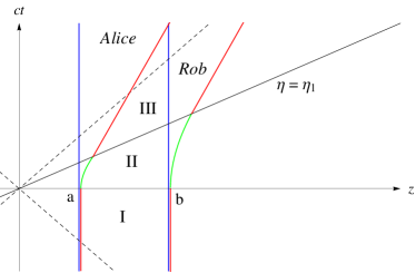
Figure 1: Space-time diagram of cavity motion is shown. Rob’s cavity is at rest initially (Region $\mathrm{I}$), then undergoes a period of uniform acceleration from $t=0$ to $\eta=\eta_{1}$ (Region $\mathrm{I\!I}$) and is thereafter again inertial (Region $\mathrm{I\!I\!I}$). Alice’s cavity overlaps with Rob’s cavity in Region $\mathrm{I}$ and remains inertial throughout.

We shall discuss the evolution in Rob’s cavity in two steps: first from Region $\mathrm{I}$ to Region $\mathrm{I\!I}$ and then from Region $\mathrm{I\!I}$ to Region $\mathrm{I\!I\!I}$. We then use the evolution to relate the operators and the vacuum of Region $\mathrm{I}$ to those in Region $\mathrm{I\!I\!I}$.

III.1 Region $\mathrm{I}$ to Region $\mathrm{I\!I}$

Consider the Dirac field in Rob’s cavity. In Regions $\mathrm{I}$ and $\mathrm{I\!I}$ we may expand the field using the solutions (7) and (11) respectively as

$$\mathrm{I}:\ \ \ \psi =\sum\limits_{n\geq 0}a_{n}\,\psi_{n}\,+\,\sum\limits_{n<0}b_{n}^{\dagger}\,\psi_{n}\ ,$$ (12a)

$$\mathrm{I\!I}:\ \ \ \psi =\sum\limits_{m\geq 0}\widehat{a}_{m}\,\widehat{\psi}_{m}\,+\,\sum\limits_{m<0}\widehat{b}_{m}^{\dagger}\,\widehat{\psi}_{m}\ ,$$ (12b)

where the nonvanishing anticommutators are

$$\mathrm{I}:\ \ \ \left\{a_{m},a_{n}^{\dagger}\right\}=\left\{b_{m},b_{n}^{\dagger}\right\}=\delta_{mn}\,,$$ (13a)

$$\mathrm{I\!I}:\ \ \ \left\{\widehat{a}_{m},\widehat{a}_{n}^{\dagger}\right\}=\left\{\widehat{b}_{m},\widehat{b}_{n}^{\dagger}\right\}=\delta_{mn}\,.$$ (13b)

Matching the expansions (12) at $t=0$, we have the Bogoliubov transformation

$$\widehat{\psi}_{m}=\sum\limits_{n}A_{mn}\,\psi_{n}\ ,\ \ \ \psi_{n}=\sum\limits_{m}A_{mn}^{*}\,\widehat{\psi}_{m}\,,$$ (14)

where the elements of the Bogoliubov coefficient matrix $A=\left(A_{mn}\right)$ are given by

$$A_{mn}\,=\,\bigl{(}\,\psi_{n},\widehat{\psi}_{m}\,\bigr{)}$$ (15)

and the inner product in (15) is evaluated on the surface $t=0$. Note that $A$ is unitary by construction.

We shall be working perturbatively in the limit where the acceleration of Rob’s cavity is small. To implement this, we follow bruschifuenteslouko11 and introduce the dimensionless parameter $h:=2\delta/(a+b)$, satisfying $0<h<2$. Physically, $h$ is the product of the cavity’s length $\delta$ and the acceleration at the centre of the cavity. Expanding (15) in a Maclaurin series in $h$, we find

$$A=A^{(0)}\,+\,A^{(1)}\,+\,A^{(2)}\,+\,{O}(h^{3})\ ,$$ (16)

where the superscript indicates the power of $h$ and the explicit expressions for $A^{(0)}$, $A^{(1)}$ and $A^{(2)}$ read

$$A_{mn}^{(0)} =\delta_{mn}\,,$$ (17a)

$$A_{nn}^{(1)} =0\,,$$ (17b)

$$A_{mn}^{(1)} =\frac{\bigl{[}(-1)^{m+n}-1\bigr{]}(m+n+2s)}{2\pi^{2}(m-n)^{3}}\,h\,,\ \ \ (m\neq n)$$ (17c)

$$A_{nn}^{(2)} =-\left(\frac{1}{96}+\frac{\pi^{2}(n+s)^{2}}{240}\right)h^{2}\,,$$ (17d)

$$A_{mn}^{(2)} =\frac{\bigl{[}(-1)^{m+n}+1\bigr{]}}{8\pi^{2}(m-n)^{4}}\bigl{[}(m+s)^{2}+3(n+s)^{2}$$

$$\hskip 38.74988pt+8(m+s)(n+s)\bigr{]}h^{2}\,.\ \ \ (m\neq n)$$ (17e)

The expressions (17) show that the small $h$ expansion of $A_{mn}$ is not uniform in the indices, but we have verified that the expansion maintains the unitarity of $A$ perturbatively to order $h^{2}$ and the products of the order $h$ matrices in the unitarity identities are unconditionally convergent.

The perturbative unitarity of $A$ persists in the limit $s\to 0_{+}$. Had we set $s=0$ at the outset and dropped the zero mode from the system by hand, the resulting truncated $A$ would not be perturbatively unitary to order $h^{2}$.

III.2 Region $\mathrm{I}$ to Region $\mathrm{I\!I\!I}$

In Region $\mathrm{I\!I\!I}$, we expand the Dirac field in Rob’s cavity as

$$\mathrm{I\!I\!I}:\ \ \ \psi =\sum\limits_{n\geq 0}\tilde{a}_{n}\,\tilde{\psi}_{n}\,+\,\sum\limits_{n<0}\tilde{b}_{n}^{\dagger}\,\tilde{\psi}_{n}\ ,$$ (18)

where the mode functions $\tilde{\psi}_{n}$ are as in (7) but $(t,z)$ are replaced by the Minkowski coordinates $(\tilde{t},\tilde{z})$ adapted to the cavity’s new rest frame, with the surface $\tilde{t}=0$ coinciding with $\eta=\eta_{1}$. The nonvanishing anticommutators are

$$\mathrm{I\!I\!I}:\ \ \ \left\{\tilde{a}_{m},\tilde{a}_{n}^{\dagger}\right\}=\left\{\tilde{b}_{m},\tilde{b}_{n}^{\dagger}\right\}=\delta_{mn}\,.$$ (19)

The Bogoliubov transformation between the Region $\mathrm{I}$ and Region $\mathrm{I\!I\!I}$ modes can then be written as

$$\tilde{\psi}_{m}=\sum\limits_{n}\mathcal{A}_{mn}\,\psi_{n}\ ,\ \ \ \psi_{n}=\sum\limits_{m}\mathcal{A}_{mn}^{*}\,\tilde{\psi}_{m}\,,$$ (20)

where the coefficient matrix $\mathcal{A}=\left(\mathcal{A}_{mn}\right)$ has the decomposition

$$\mathcal{A}=A^{\dagger}\,G(\eta_{1})\,A$$ (21)

and $G(\eta_{1})$ is the diagonal matrix whose diagonal elements are

$$G_{nn}(\eta_{1})=\exp(i\,\Omega_{n}\,\eta_{1})=:G_{n}\,.$$ (22)

The role of $G(\eta_{1})$ in (21) is to compensate for the phases that the modes $\widehat{\psi}_{m}$ develop between $\eta=0$ and $\eta=\eta_{1}$, and the matrix $A^{\dagger}=A^{-1}$ in (21) arises from matching Region $\mathrm{I\!I}$ to Region $\mathrm{I\!I\!I}$ at $\eta=\eta_{1}$. Note that $\mathcal{A}$ is unitary by construction.

Expanding $\mathcal{A}$ in a Maclaurin series in $h$ as

$$\mathcal{A}=\mathcal{A}^{(0)}\,+\,\mathcal{A}^{(1)}\,+\,\mathcal{A}^{(2)}\,+\,{O}(h^{3})\ ,$$ (23)

where the superscript again indicates the power of $h$, we obtain from (16) and (21)

$$\mathcal{A}^{(0)} =G(\eta_{1})\,,$$ (24a)

$$\mathcal{A}^{(1)} =G(\eta_{1})\,A^{(1)}+\bigl{(}A^{(1)}\bigr{)}^{\dagger}G(\eta_{1})\,,$$ (24b)

$$\mathcal{A}^{(2)} =G(\eta_{1})\,A^{(2)}+\bigl{(}A^{(2)}\bigr{)}^{\dagger}G(\eta_{1})+\bigl{(}A^{(1)}\bigr{)}^{\dagger}G(\eta_{1})\,A^{(1)}\,.$$ (24c)

Note that the diagonal elements of $\mathcal{A}^{(1)}$ are vanishing. Unitarity of $\mathcal{A}$ implies the perturbative relations

$$0 =G(\eta_{1})^{*}\mathcal{A}^{(1)}+\bigl{(}\mathcal{A}^{(1)}\bigr{)}^{\dagger}G(\eta_{1})\,,$$ (25a)

$$0 =G(\eta_{1})^{*}\mathcal{A}^{(2)}+\bigl{(}\mathcal{A}^{(2)}\bigr{)}^{\dagger}G(\eta_{1})+\bigl{(}\mathcal{A}^{(1)}\bigr{)}^{\dagger}\mathcal{A}^{(1)}\,,$$ (25b)

which will be useful below.

III.3 Operators and vacua

We denote the Fock vacua in Regions $\mathrm{I}$ and $\mathrm{I\!I\!I}$ by $\left|\,0\,\right\rangle$ and $\left|\,\tilde{0}\,\right\rangle$ respectively. To relate the two, we mimic the bosonic case fabbrinavarrosalas and make the ansatz

$$\left|\,0\,\right\rangle\,=\,Ne^{W}\left|\,\tilde{0}\,\right\rangle\,,$$ (26)

where

$$W\,=\,\sum\limits_{p\geq 0,q<0}\,V_{pq}\,\tilde{a}_{p}^{\dagger}\,\tilde{b}_{q}^{\dagger}$$ (27)

and the coefficient matrix $V=\left(V_{pq}\right)$ and the normalisation constant $N$ are to be determined. Note that the two indices of $V$ take values in disjoint sets.

It follows from (12a), (18) and (20) that the creation and annihilation operators in Regions $\mathrm{I}$ and $\mathrm{I\!I\!I}$ are related by

$$n\geq 0:\ a_{n} =\left(\,\psi_{n},\psi\,\right)=\sum\limits_{m\geq 0}\tilde{a}_{m}\,\mathcal{A}_{mn}\,+\,\sum\limits_{m<0}\tilde{b}_{m}^{\dagger}\,\mathcal{A}_{mn}\ ,$$ (28a)

$$n<0:\ b_{n}^{\dagger} =\left(\,\psi_{n},\psi\,\right)=\sum\limits_{m\geq 0}\tilde{a}_{m}\,\mathcal{A}_{mn}\,+\,\sum\limits_{m<0}\tilde{b}_{m}^{\dagger}\,\mathcal{A}_{mn}\ .$$ (28b)

Using (26) and (28a), the condition $a_{n}\left|\,0\,\right\rangle=0$ reads

$$\Biggl{(}\,\sum\limits_{m\geq 0}\tilde{a}_{m}\,\mathcal{A}_{mn}+\sum\limits_{m<0}\tilde{b}_{m}^{\dagger}\,\mathcal{A}_{mn}\Biggr{)}e^{W}\left|\,\tilde{0}\,\right\rangle=0\,.$$ (29)

From the anticommutators (19) it follows that

$$\left[\,W\,,\,\tilde{a}_{m}\,\right]\,=\,-\sum\limits_{q<0}V_{mq}\,\tilde{b}_{q}^{\dagger}\,,$$ (30a)

$$\left[\,W\,,\,\left[\,W\,,\,\tilde{a}_{m}\,\right]\,\right]\,=\,0\,.$$ (30b)

Using (30) and the Hadamard lemma,

$$e^{A}\,Be^{-A}\,=\,B\,+\,\left[\,A\,,\,B\,\right]\,+\,\tfrac{1}{2}\left[\,A\,,\,\left[\,A\,,\,B\,\right]\,\right]\,+\,\ldots,$$ (31)

(29) reduces to

$$\sum\limits_{m\geq 0}\mathcal{A}_{mn}\,V_{mq}\,=\,-\,\mathcal{A}_{qn}\ \ \ (n\,\geq\,0\,,\ q\,<\,0)\ .$$ (32)

A similar computation shows that the condition $b_{n}\,\left|\,0\,\right\rangle=0$ reduces to

$$\sum\limits_{m<0}\mathcal{A}_{mn}^{*}\,V_{pm}\,=\,\,\mathcal{A}_{pn}^{*}\ \ \ (n\,<\,0\,,\ p\,\geq\,0)\ .$$ (33)

If the block of $\mathcal{A}$ where both indices are non-negative is invertible, Eq. (32) determines $V$ uniquely. Similarly, if the block of $\mathcal{A}$ where both indices are negative is invertible, Eq. (33) determines $V$ uniquely. If both blocks are invertible, it can be verified using unitarity of $\mathcal{A}$ that the ensuing two expressions for $V$ are equivalent. Working perturbatively in $h$, the invertibility assumptions hold, and using (23) and (24) we find

$$V\,=\,V^{(1)}\,+\,{O}(h^{2})$$ (34)

where

$$V_{pq}^{(1)}\,=\,-\mathcal{A}_{qp}^{(1)}\,G_{p}^{\,*}\,=\,\mathcal{A}_{pq}^{(1)*}\,G_{q}\,\ \ (p\geq 0,\ q<0).$$ (35)

We shall show in Section IV that the normalisation constant $N$ has the small $h$ expansion

$$N\,=\,1\,-\,\tfrac{1}{2}\sum\limits_{p,q}|V_{pq}|^{2}\ +{O}(h^{3})\,.$$ (36)

IV Evolution of entangled states

In this section we apply the results of Section III to the evolution of Bell-type quantum states between the two cavities which are initially maximally entangled. We shall work perturbatively to quadratic order in $h$.

Focusing first on Rob’s cavity only, we write out in Sec. IV.1 the Region $\mathrm{I}$ vacuum and the Region $\mathrm{I}$ states with a single (anti-)particle in terms of Region $\mathrm{I\!I\!I}$ excitations on the Region $\mathrm{I\!I\!I}$ vacuum. In Sec. IV.2 we address an entangled state where one field mode is controlled by Alice and one by Rob. In Sec. IV.3 we address a state of the type analysed in martinmartinezfuentes11 where the entanglement between Alice and Rob is in the charge of the field modes.

IV.1 Rob’s cavity: vacuum and single-particle states

Consider the Region $\mathrm{I}$ vacuum $\left|\,0\,\right\rangle$ in Rob’s cavity. We shall use (26) to express this state in terms of Region $\mathrm{I\!I\!I}$ excitations over the Region $\mathrm{I\!I\!I}$ vacuum $\left|\,\tilde{0}\,\right\rangle$.

We expand the exponential in (26) as

$$e^{W} =\mathds{1}\,+\,\sum\limits_{p,q}V_{pq}\,\tilde{a}_{p}^{\dagger}\,\tilde{b}_{q}^{\dagger}$$

$$\hskip 21.52771pt+\tfrac{1}{2}\,\sum\limits_{p,q,i,j}V_{pq}\,V_{ij}\,\tilde{a}_{p}^{\dagger}\,\tilde{b}_{q}^{\dagger}\,\tilde{a}_{i}^{\dagger}\,\tilde{b}_{j}^{\dagger}\,+\,{O}(h^{3})\,.$$ (37)

We denote the Region $\mathrm{I\!I\!I}$ single-particle states by

$$\left|\tilde{1}_{k}\right\rangle^{\!+}:=\tilde{a}_{k}^{\dagger}\left|\,\tilde{0}\,\right\rangle$$ (38)

for $k\geq 0$ and by

$$\left|\tilde{1}_{k}\right\rangle^{\!-}:=\tilde{b}_{k}^{\dagger}\left|\,\tilde{0}\,\right\rangle$$ (39)

for $k<0$, so that the superscript $\pm$ indicates the sign of the charge. From (37) we obtain

$$e^{W}\,\left|\,\tilde{0}\,\right\rangle =\left|\,\tilde{0}\,\right\rangle\,+\,\sum\limits_{p,q}V_{pq}\,\left|\,\tilde{1}_{p}\right\rangle^{+}\,\left|\tilde{1}_{q}\,\right\rangle^{-}$$

$$\hskip 4.30554pt-\tfrac{1}{2}\sum\limits_{p,q,i,j}V_{pq}V_{ij}(1-\delta_{pi})(1-\delta_{qj})\times$$

$$\hskip 25.83325pt\times\left|\tilde{1}_{p}\right\rangle^{\!+}\left|\tilde{1}_{i}\right\rangle^{\!+}\left|\tilde{1}_{q}\right\rangle^{\!-}\left|\tilde{1}_{j}\right\rangle^{\!-}+{O}(h^{3})\,,$$ (40)

where the ordering of the single-particle kets encodes the ordering of the fermion creation operators. It follows that the normalisation constant $N$ is given by (36), and (26) gives

$$\left|\,0\,\right\rangle =\Bigl{(}1\,-\,\tfrac{1}{2}\sum\limits_{p,q}|V_{pq}|^{2}\Bigr{)}\left|\,\tilde{0}\,\right\rangle\,+\,\sum\limits_{p,q}V_{pq}\,\left|\,\tilde{1}_{p}\right\rangle^{+}\,\left|\tilde{1}_{q}\,\right\rangle^{-}$$

$$\hskip 4.30554pt-\tfrac{1}{2}\sum\limits_{p,q,i,j}V_{pq}V_{ij}(1-\delta_{pi})(1-\delta_{qj})\times$$

$$\hskip 25.83325pt\times\left|\tilde{1}_{p}\right\rangle^{\!+}\left|\tilde{1}_{i}\right\rangle^{\!+}\left|\tilde{1}_{q}\right\rangle^{\!-}\left|\tilde{1}_{j}\right\rangle^{\!-}+{O}(h^{3})\,.$$ (41)

Consider then in Rob’s cavity the state with exactly one Region $\mathrm{I}$ particle, $\left|1_{k}\right\rangle^{\!-}:={b}_{k}^{\dagger}\left|\,0\,\right\rangle$ for $k<0$ or $\left|1_{k}\right\rangle^{\!+}:={a}_{k}^{\dagger}\left|\,0\,\right\rangle$ for $k\geq 0$. Acting on the Region $\mathrm{I}$ vacuum (41) by (28b) and the Hermitian conjugate of (28a) respectively, we find

$$k<0:\ \ \ \left|1_{k}\right\rangle^{\!-}=\sum\limits_{p,q}V_{pq}\mathcal{A}_{pk}\left|\tilde{1}_{q}\right\rangle^{\!-}+\sum\limits_{m<0}\mathcal{A}_{mk}\Biggl{[}\Bigl{(}1-\tfrac{1}{2}\sum\limits_{p,q}|V_{pq}|^{2}\Bigr{)}\left|\tilde{1}_{m}\right\rangle^{\!-}+\sum\limits_{p,q}V_{pq}(1-\delta_{mq})\left|\tilde{1}_{p}\right\rangle^{\!+}\!\left|\tilde{1}_{q}\right\rangle^{\!-}\!\left|\tilde{1}_{m}\right\rangle^{\!-}$$

$$\hskip 86.11084pt-\tfrac{1}{2}\sum\limits_{p,q,i,j}V_{pq}V_{ij}(1\!-\!\delta_{pi})(1\!-\!\delta_{qj})(1\!-\!\delta_{mq})(1\!-\!\delta_{mj})\left|\tilde{1}_{p}\right\rangle^{\!+}\!\left|\tilde{1}_{i}\right\rangle^{\!+}\!\left|\tilde{1}_{q}\right\rangle^{\!-}\!\left|\tilde{1}_{j}\right\rangle^{\!-}\!\left|\tilde{1}_{m}\right\rangle^{\!-}\Biggr{]}+{O}(h^{3})\,,$$ (42a)

$$k>0:\ \ \ \left|1_{k}\right\rangle^{\!+}=-\sum\limits_{p,q}V_{pq}\mathcal{A}_{qk}^{*}\left|\tilde{1}_{p}\right\rangle^{\!+}+\sum\limits_{m\geq 0}\mathcal{A}_{mk}^{*}\Biggl{[}\Bigl{(}1-\tfrac{1}{2}\sum\limits_{p,q}|V_{pq}|^{2}\Bigr{)}\left|\tilde{1}_{m}\right\rangle^{\!+}+\sum\limits_{p,q}V_{pq}\,(1-\delta_{mp})\left|\tilde{1}_{m}\right\rangle^{\!+}\!\left|\tilde{1}_{p}\right\rangle^{\!+}\!\left|\tilde{1}_{q}\right\rangle^{\!-}$$

$$\hskip 86.11084pt-\tfrac{1}{2}\sum\limits_{p,q,i,j}V_{pq}V_{ij}(1\!-\!\delta_{pi})(1\!-\!\delta_{qj})(1\!-\!\delta_{mp})(1\!-\!\delta_{mi})\left|\tilde{1}_{m}\right\rangle^{\!+}\!\left|\tilde{1}_{p}\right\rangle^{\!+}\!\left|\tilde{1}_{i}\right\rangle^{\!+}\!\left|\tilde{1}_{q}\right\rangle^{\!-}\!\left|\tilde{1}_{j}\right\rangle^{\!-}\Biggr{]}+{O}(h^{3})\,.$$ (42b)

IV.2 Entangled two-mode states

We wish to consider a Region $\mathrm{I}$ state where one field mode is controlled by Alice and one by Rob. Concretely, we take

$$\left|\,\phi^{\pm}_{\text{init}}\,\right\rangle_{AR+} =\tfrac{1}{\sqrt{2}}\left(\,\left|\,0_{\hat{k}}\,\right\rangle_{A}\left|\,0_{k}\,\right\rangle_{R}\,\pm\,\left|\,1_{\hat{k}}\,\right\rangle_{A}^{\kappa}\left|\,1_{k}\,\right\rangle_{R}^{+}\,\right),$$ (43a)

$$\left|\,\phi^{\pm}_{\text{init}}\,\right\rangle_{AR-} =\tfrac{1}{\sqrt{2}}\left(\,\left|\,0_{\hat{k}}\,\right\rangle_{A}\left|\,0_{k}\,\right\rangle_{R}\,\pm\,\left|\,1_{\hat{k}}\,\right\rangle_{A}^{\kappa}\left|\,1_{k}\,\right\rangle_{R}^{-}\,\right),$$ (43b)

where the subscripts $A$ and $R$ refer to the cavity and the superscripts $\pm$ indicate whether the mode has positive or negative frequency, so that $\kappa=+$ for $\hat{k}\geq 0$ and $\kappa=-$ for $\hat{k}<0$. Furthermore, we consider the two particle basis state of the two mode Hilbert space, corresponding to one excitation each in the modes $\hat{k}$ in Alice’s cavity and $k$ in Rob’s cavity, to be ordered as in (43). As pointed out in Ref. monteromartinmartinez11 , making such a choice can lead to ambiguities in the entanglement. In our case, the ambiguity amounts to a relative phase shift of $\pi$, i.e., a sign change, in (43), which does not affect the amount of entanglement. In other words, the states (43) are pure, bipartite, maximally entangled states of mode $\hat{k}$ in Alice’s cavity and mode $k$ in Rob’s cavity.

We form the density matrix for each of the states (43), express the density matrix in terms of Rob’s Region $\mathrm{I\!I\!I}$ basis to order $h^{2}$ using (41) and (42), and take the partial trace over all of Rob’s modes except the reference mode $k$. All of Rob’s modes except $k$ are thus regarded as environment, to which information is lost due to the acceleration. The relevant partial traces of Rob’s matrix elements depend on the sign of the mode label $k$. For $k\geq\,0$, corresponding to (43a), we find

$$\textnormal{Tr}_{\lnot k}\left|\,0_{k}\right\rangle\left\langle\,0_{k}\right| =(1-f_{k}^{-})\left|\,\tilde{0}_{k}\right\rangle\left\langle\tilde{0}_{k}\right|+f_{k}^{-}\left|\tilde{1}_{k}\right\rangle^{\!\!++\!\!}\!\left\langle\tilde{1}_{k}\right|,$$ (44a)

$$\textnormal{Tr}_{\lnot k}\left|\,0_{k}\right\rangle^{+}\!\!\!\left\langle 1_{k}\right| =\Bigl{(}G_{k}+\mathcal{A}_{kk}^{(2)}\Bigr{)}\left|\,\tilde{0}_{k}\right\rangle^{+}\!\!\!\left\langle\tilde{1}_{k}\right|,$$ (44b)

$$\textnormal{Tr}_{\lnot k}\left|1_{k}\right\rangle^{\!\!++\!\!}\!\left\langle 1_{k}\right| =(1-f_{k}^{+})\left|\tilde{1}_{k}\right\rangle^{\!\!++\!\!}\!\left\langle\tilde{1}_{k}\right|+f_{k}^{+}\left|\,\tilde{0}_{k}\right\rangle\left\langle\tilde{0}_{k}\right|,$$ (44c)

where we have used (25a) and (35) and introduced the abbreviations

$$f_{k}^{+}:=\sum\limits_{p\geq 0}\bigl{|}\mathcal{A}_{pk}^{(1)}\bigr{|}^{2}\,,\ \ \ \ f_{k}^{-}:=\sum\limits_{q<0}\bigl{|}\mathcal{A}_{qk}^{(1)}\bigr{|}^{2}\,.$$ (45)

For $k<0$, corresponding to (43b), we find similarly

$$\textnormal{Tr}_{\lnot k}\left|\,0_{k}\right\rangle\left\langle\,0_{k}\right| =(1-f_{k}^{+})\left|\,\tilde{0}_{k}\right\rangle\left\langle\tilde{0}_{k}\right|+f_{k}^{+}\left|\tilde{1}_{k}\right\rangle^{\!\!--\!\!}\!\left\langle\tilde{1}_{k}\right|,$$ (46a)

$$\textnormal{Tr}_{\lnot k}\left|\,0_{k}\right\rangle^{-}\!\!\!\left\langle 1_{k}\right| =\Bigl{(}G_{k}^{\,*}+\mathcal{A}_{kk}^{(2)*}\bigr{)}\left|\,\tilde{0}_{k}\right\rangle^{-}\!\!\!\left\langle\tilde{1}_{k}\right|,$$ (46b)

$$\textnormal{Tr}_{\lnot k}\left|1_{k}\right\rangle^{\!\!--\!\!}\!\left\langle 1_{k}\right| =(1-f_{k}^{-})\left|\tilde{1}_{k}\right\rangle^{\!\!--\!\!}\!\left\langle\tilde{1}_{k}\right|+f_{k}^{-}\left|\,\tilde{0}_{k}\right\rangle\left\langle\tilde{0}_{k}\right|.$$ (46c)

IV.3 States with entanglement between opposite charges

We finally consider the Region $\mathrm{I}$ state

$$\left|\,\chi^{\pm}_{\text{init}}\,\right\rangle_{AR}\,=\,\tfrac{1}{\sqrt{2}}\left(\,\left|\,1_{k}\,\right\rangle_{A}^{\!+}\left|\,1_{k^{\prime}}\,\right\rangle_{R}^{\!-}\,\pm\,\left|\,1_{k^{\prime}}\,\right\rangle_{A}^{\!-}\left|\,1_{k}\,\right\rangle_{R}^{\!+}\,\right),$$ (47)

where the meaning of the subscripts and superscripts is as described for Eq. (43), indicating that $k\geq 0$ and $k^{\prime}<0$. In this state Alice and Rob each have access to both of the modes $k$ and $k^{\prime}$, and the entanglement is in the charge of the field modes, similarly to the states considered in martinmartinezfuentes11 .

We form the reduced density matrix to order $h^{2}$ as in Sec. IV.2, but now the partial tracing over Rob’s modes excludes both mode $k$ and mode $k^{\prime}$. The relevant matrix elements take the form

$$\textnormal{Tr}_{\lnot k,k^{\prime}}\left|1_{k^{\prime}}\right\rangle^{\!\!--\!\!}\!\left\langle 1_{k^{\prime}}\right|\ =\ f_{k^{\prime}}^{-}\left|\,\tilde{0}_{k}\right\rangle^{\!\!+}\!\left|\,\tilde{0}_{k^{\prime}}\right\rangle^{\!\!--\!\!}\!\left\langle\tilde{0}_{k^{\prime}}\right|^{+\!\!}\!\left\langle\tilde{0}_{k}\right|$$

$$\ +\,\bigl{(}1\!-\!f_{k^{\prime}}^{-}\!-\!f_{k}^{-}\!+\!\bigl{|}\mathcal{A}_{kk^{\prime}}^{(1)}\bigr{|}^{2}\bigr{)}\left|\,\tilde{0}_{k}\right\rangle^{\!\!+}\!\left|\,\tilde{1}_{k^{\prime}}\right\rangle^{\!\!--\!\!}\!\left\langle\tilde{1}_{k^{\prime}}\right|^{+\!\!}\!\left\langle\tilde{0}_{k}\right|$$

$$\ +\,\bigl{(}f_{k}^{-}\!-\!\bigl{|}\mathcal{A}_{kk^{\prime}}^{(1)}\bigr{|}^{2}\bigr{)}\left|\,\tilde{1}_{k}\right\rangle^{\!\!+}\!\left|\,\tilde{1}_{k^{\prime}}\right\rangle^{\!\!--\!\!}\!\left\langle\tilde{1}_{k^{\prime}}\right|^{+\!\!}\!\left\langle\tilde{1}_{k}\right|$$

$$\ +\,\Bigl{(}\sum\limits_{q<0}G_{k}G_{k^{\prime}}^{\,*}\mathcal{A}_{qk}^{(1)*}\mathcal{A}_{qk^{\prime}}^{(1)}\left|\,\tilde{0}_{k}\right\rangle^{\!\!+}\!\left|\,\tilde{0}_{k^{\prime}}\right\rangle^{\!\!--\!\!}\!\left\langle\tilde{1}_{k^{\prime}}\right|^{+\!\!}\!\left\langle\tilde{1}_{k}\right|$$

$$\ \hskip 21.52771pt\,+\,h.c.\Bigr{)}\,,$$ (48a)

$$\textnormal{Tr}_{\lnot k,k^{\prime}}\left|1_{k}\,\right\rangle^{\!\!++\!\!}\!\left\langle 1_{k}\,\right|\ =\ f_{k}^{+}\left|\,\tilde{0}_{k}\right\rangle^{\!\!+}\!\left|\,\tilde{0}_{k^{\prime}}\right\rangle^{\!\!--\!\!}\!\left\langle\tilde{0}_{k^{\prime}}\right|^{+\!\!}\!\left\langle\tilde{0}_{k}\right|$$

$$\ +\,\bigl{(}1\!-\!f_{k^{\prime}}^{+}\!-\!f_{k}^{+}\!+\!\bigl{|}\mathcal{A}_{kk^{\prime}}^{(1)}\bigr{|}^{2}\bigr{)}\left|\,\tilde{1}_{k}\right\rangle^{\!\!+}\!\left|\,\tilde{0}_{k^{\prime}}\right\rangle^{\!\!--\!\!}\!\left\langle\tilde{0}_{k^{\prime}}\right|^{+\!\!}\!\left\langle\tilde{1}_{k}\right|$$

$$\ +\,\bigl{(}f_{k^{\prime}}^{+}\!-\!\bigl{|}\mathcal{A}_{kk^{\prime}}^{(1)}\bigr{|}^{2}\bigr{)}\left|\,\tilde{1}_{k}\right\rangle^{\!\!+}\!\left|\,\tilde{1}_{k^{\prime}}\right\rangle^{\!\!--\!\!}\!\left\langle\tilde{1}_{k^{\prime}}\right|^{+\!\!}\!\left\langle\tilde{1}_{k}\right|$$

$$\ -\,\Bigl{(}\sum\limits_{p\geq 0}G_{k}G_{k^{\prime}}^{\,*}\mathcal{A}_{pk}^{(1)*}\mathcal{A}_{pk^{\prime}}^{(1)}\left|\,\tilde{0}_{k}\right\rangle^{\!\!+}\!\left|\,\tilde{0}_{k^{\prime}}\right\rangle^{\!\!--\!\!}\!\left\langle\tilde{1}_{k^{\prime}}\right|^{+\!\!}\!\left\langle\tilde{1}_{k}\right|$$

$$\ \hskip 21.52771pt\,+\,h.c.\Bigr{)}\,,$$ (48b)

$$\textnormal{Tr}_{\lnot k,k^{\prime}}\left|1_{k}\,\right\rangle^{\!\!+-\!\!}\!\left\langle 1_{k^{\prime}}\,\right|=\Bigl{(}G_{k}^{\,*}G_{k^{\prime}}^{\,*}\bigl{|}\mathcal{A}_{kk^{\prime}}^{(1)}\bigr{|}^{2}$$

$$\ \ +\mathcal{A}_{kk}^{*}\mathcal{A}_{k^{\prime}k^{\prime}}^{*}\Bigr{)}\left|\,\tilde{1}_{k}\right\rangle^{\!\!+}\!\left|\,\tilde{0}_{k^{\prime}}\right\rangle^{\!\!--\!\!}\!\left\langle\tilde{1}_{k^{\prime}}\right|^{+\!\!}\!\left\langle\tilde{0}_{k}\right|\,,$$ (48c)

where in (48c) $\mathcal{A}_{kk}^{*}\mathcal{A}_{k^{\prime}k^{\prime}}^{*}$ is kept only to order $h^{2}$ in the small $h$ expansion

$$\mathcal{A}_{kk}^{*}\mathcal{A}_{k^{\prime}k^{\prime}}^{*}\,=\,G_{k}^{\,*}G_{k^{\prime}}^{\,*}+G_{k^{\prime}}^{\,*}\mathcal{A}_{kk}^{(2)*}+G_{k}^{\,*}\mathcal{A}_{k^{\prime}k^{\prime}}^{(2)*}+{O}(h^{3})\,.$$ (49)

V Entanglement degradation and nonlocality

We are now in a position to study the entanglement and the nonlocality of our states in Region $\mathrm{I\!I\!I}$.

V.1 Entanglement of two-mode states

Consider the states $\left|\,\phi^{\pm}_{\text{init}}\,\right\rangle_{AR+}$ and $\left|\,\phi^{\pm}_{\text{init}}\,\right\rangle_{AR-}$ (43), in which Alice and Rob control one mode each. We shall quantify the entanglement by the negativity vidalwerner02 ; audenaert-etal ; plenio-virmani:review and the nonlocality by a possible violation of the CHSH inequality chsh69 ; horodecki-rpm95 .

The negativity $\mathcal{N}[\rho]$ is an entanglement monotone that quantifies how strongly the partial transpose of a density operator $\rho$ fails to be positive. It is defined as the sum of the absolute values of the negative eigenvalues $\lambda$ of $(\mathds{1}\otimes T_{R})\rho$,

$$\mathcal{N}[\rho]\,=\,\sum\limits_{\lambda<0}\,|\lambda|\ ,$$ (50)

where $(\mathds{1}\otimes T_{R})$ denotes the transpose in one of the two subsystems (which we have taken to be Rob without loss of generality). The negativity is a useful measure for our system because all the entangled states that it fails to detect are necessarily bound entangled, that is, these states cannot be distilled horo3-prl , and a system with two fermionic modes cannot be bound entangled.

We work perturbatively in $h$. The unperturbed part of $(\mathds{1}\otimes T_{R})\rho_{AR\pm}^{\pm}$ has the triply degenerate eigenvalue $\tfrac{1}{2}$ and the nondegenerate eigenvalue $-\tfrac{1}{2}$. In a perturbative treatment the positive eigenvalues remain positive and the only correction to the negativity comes from the perturbative correction to the negative eigenvalue. A straightforward computation using (44) and (46) shows that the leading correction to the negativity comes in order $h^{2}$, and to this order the negativity formula reads

$$\mathcal{N}[\rho^{\pm}_{AR\pm}]\,=\,\tfrac{1}{2}\left(1-f_{k}\right)$$ (51)

where $f_{k}:=f_{k}^{+}+f_{k}^{-}$. $f_{k}$ can be expressed as

$$f_{k} =\sum\limits_{p=-\infty}^{\infty}\bigl{|}E_{1}^{k-p}-1\bigr{|}^{2}\bigl{|}A_{kp}^{(1)}\bigr{|}^{2}$$

$$=2\bigl{[}Q(2k+s,1)-Q(2k+s,E_{1})\bigr{]}h^{2}$$ (52)

where

$$Q(\alpha,z) :=\frac{2}{\pi^{4}}\operatorname{Re}\biggl{[}\alpha^{2}\left(\operatorname{Li}_{6}(z)-\frac{1}{64}\operatorname{Li}_{6}(z^{2})\right)$$

$$\hskip 38.74988pt+\operatorname{Li}_{4}(z)-\frac{1}{16}\operatorname{Li}_{4}(z^{2})\biggr{]},$$ (53)

$\operatorname{Li}$ is the polylogarithm nist-dig-library and

$$E_{1}:=\exp\!\left(\frac{i\pi\eta_{1}}{\ln(b/a)}\right)=\exp\!\left(\frac{i\pi h\tau_{1}}{2\delta\operatorname{atanh}(h/2)}\right).$$ (54)

We see from (51) that acceleration does degrade the initially maximal entanglement, and the degradation is determined by the function $f_{k}$ (52). $f_{k}$ is periodic in $\tau_{1}$ with period $2\delta{(h/2)}^{-1}\operatorname{atanh}(h/2)$, which is the proper time measured at the centre of Rob’s cavity between sending and recapturing a light ray that is allowed to bounce off each wall once. $f_{k}$ is non-negative, and it vanishes only at integer multiples of the period. $f_{k}$ is not even in $k$ for generic values of $s$, but it is even in $k$ in the limiting case $s=0$ in which the spectrum is symmetric between positive and negative charges. $f_{k}$ diverges at large $|k|$ proportionally to $k^{2}$, and the domain of validity of our perturbative analysis is $|k|h\ll 1$. Plots for $k=\pm 1$ are shown in Fig. 2.

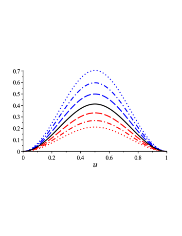
Figure 2: The plot shows $f_{k}/h^{2}$ as a function of $u:=\tfrac{1}{2}\eta_{1}/\ln(b/a)=h\tau_{1}/\bigl{[}4\delta\operatorname{atanh}(h/2)\bigr{]}$, over the full period $0\leq u\leq 1$. The solid curve (black) is for $s=0$ with $k=\pm 1$. The dashed, dash-dotted and dotted curves are respectively for $s=\frac{1}{4}$, $s=\frac{1}{2}$ and $s=\frac{3}{4}$, for $k=1$ (blue) above the solid curve and for $k=-1$ (red) below the solid curve.

Another, potentially useful measure of entanglement for the states at hand would be the concurrence wootters98 . While a perturbative computation of the concurrence would as such be feasible, we have verified that obtaining the leading order correction would require expanding the states (42) to order $h^{4}$. We have not pursued this expansion.

We now turn to nonlocality, as quantified by the violation of the CHSH inequality chsh69 ; horodecki-rpm95

$$|\left\langle\,\mathcal{B}_{\text{CHSH}}\,\right\rangle_{\rho}|\,\leq\,2\,,$$ (55)

where $\mathcal{B}_{\text{CHSH}}$ is the bipartite observable

$$\mathcal{B}_{\text{CHSH}}:=\mathbf{a}\cdot\mathbf{\sigma}\otimes(\mathbf{b}+\mathbf{b^{\prime}})\cdot\mathbf{\sigma}+\mathbf{a^{\prime}}\cdot\mathbf{\sigma}\otimes(\mathbf{b}-\mathbf{b^{\prime}})\cdot\mathbf{\sigma}\,,$$ (56)

$\mathbf{a}$, $\mathbf{a^{\prime}}$, $\mathbf{b}$ and $\mathbf{b^{\prime}}$ are unit vectors in $\mathbb{R}^{3}$, and $\mathbf{\sigma}$ is the vector of the Pauli matrices. The inequality (55) is satisfied by all local realistic theories, but quantum mechanics allows the left-hand side to take values up to $2\sqrt{2}$. The violation of (55) is hence a sufficient (although not necessary friiskoehlermartinmartinezbertlmann11 ; smithmann11 ) condition for the quantum state to be entangled.

To look for violations of (55), we proceed as in friiskoehlermartinmartinezbertlmann11 , noting that the maximum value of the left-hand-side in the state $\rho$ is given by horodecki-rpm95

$$\left\langle\,\mathcal{B}_{\text{max}}\,\right\rangle_{\rho}\,=\,2\,\sqrt{\mu_{1}+\mu_{2}}\,,$$ (57)

where $\mu_{1}$ and $\mu_{2}$ are the two largest eigenvalues of the matrix $U(\rho)=T^{T}_{\rho}T_{\rho}$ and the elements of the correlation matrix $T=(t_{ij})$ are given by $t_{ij}=\textnormal{Tr}[\rho\,\sigma_{i}\otimes\sigma_{j}]$. In our scenario

$$U(\rho^{\pm}_{AR\pm})=\begin{pmatrix}1-f_{k}&0&0\\ 0&1-f_{k}&0\\ 0&0&\tfrac{1}{4}-f_{k}\\ \end{pmatrix}\ +\ {O}(h^{4})\,,$$ (58)

and working to order $h^{2}$ we hence find

$$\left\langle\,\mathcal{B}_{\text{max}}\,\right\rangle_{\rho^{\pm}_{AR\pm}}\,=\,2\,\sqrt{2}\left(\,1-\tfrac{1}{2}f_{k}\right)\,.$$ (59)

The acceleration thus degrades the initially maximal violation of the CHSH inequality, and the degradation is again determined by the function $f_{k}$.

V.2 Entanglement between opposite charges

We finally turn to the entanglement between opposite charges in the state $\left|\,\chi^{\pm}_{\text{init}}\,\right\rangle_{AR}$ (47).

Expressing the density matrix in the Region $\mathrm{I\!I\!I}$ basis, tracing over Rob’s unobserved modes and working perturbatively to order $h^{2}$, we find that the only nonvanishing elements of the reduced density matrix are within a $6\times 6$ block. Partially transposing Rob’s subsystem replaces the last lines in (48a) and (48b) by their respective conjugates and shifts the particle-antiparticle off-diagonals (48c) away from the diagonal. The only nonvanishing elements of the partial transpose are thus within an $8\times 8$ block, which decomposes further into two $3\times 3$ blocks that correspond respectively to (48a) and (48b) and the $2\times 2$ block

$$\pm\tfrac{1}{2}\begin{pmatrix}0&G_{k}G_{k^{\prime}}\bigl{|}\mathcal{A}_{kk^{\prime}}^{(1)}\bigr{|}^{2}+\mathcal{A}_{kk}\mathcal{A}_{k^{\prime}k^{\prime}}\\[4.2679pt] G_{k}^{\,*}G_{k^{\prime}}^{\,*}\bigl{|}\mathcal{A}_{kk^{\prime}}^{(1)}\bigr{|}^{2}+\mathcal{A}_{kk}^{*}\mathcal{A}_{k^{\prime}k^{\prime}}^{*}&0\\ \end{pmatrix},$$ (60)

where the off-diagonal components are kept only to order $h^{2}$ in their small $h$ expansion (49).

The only negative eigenvalue comes from the $2\times 2$ block (60). We find that the negativity is given by

$$\mathcal{N}[\rho_{\chi}^{\pm}] =\tfrac{1}{2}\,-\,\tfrac{1}{4}\,\sum\limits_{p\neq k^{\prime}}\bigl{|}\mathcal{A}_{kp}^{(1)}\bigr{|}^{2}\,-\,\tfrac{1}{4}\,\sum\limits_{p\neq k}\bigl{|}\mathcal{A}_{k^{\prime}p}^{(1)}\bigr{|}^{2}$$

$$=\tfrac{1}{2}\,-\,\tfrac{1}{4}\left(f_{k}+f_{k^{\prime}}\right)+\tfrac{1}{2}\bigl{|}E_{1}^{k-k^{\prime}}-1\bigr{|}^{2}\bigl{|}A_{kk^{\prime}}^{(1)}\bigr{|}^{2}.$$ (61)

The entanglement is hence again degraded by the acceleration, and the degradation has the same periodicity in $\tau_{1}$ as in the cases considered above. The degradation now depends however on $k$ and $k^{\prime}$ not just through the individual functions $f_{k}$ and $f_{k^{\prime}}$ but also through the term proportional to $\bigl{|}A_{kk^{\prime}}^{(1)}\bigr{|}^{2}$ in (61): this interference term is nonvanishing iff $k$ and $k^{\prime}$ have different parity, and when it is nonvanishing, it diminishes the degradation effect. In the charge-symmetric special case of $s=0$ and $k=-k^{\prime}$, the degradation coincides with that found in (51) for the two-mode states (43).

VI One-way journey

Our analysis for the Rob trajectory that comprises Regions $\mathrm{I}$, $\mathrm{I\!I}$ and $\mathrm{I\!I\!I}$ can be generalised in a straightforward way to any trajectory obtained by grafting inertial and uniformly-accelerated segments, with arbitrary durations and proper accelerations. The only delicate point is that the phase conventions of our mode functions distinguish the left boundary of the cavity from the right boundary, and in Sec. III.1 we set up the Bogoliubov transformation from Minkowski to Rindler assuming that the acceleration is to the right. It follows that the Bogoliubov transformation from Minkowski to leftward-accelerating Rindler is obtained from that in Sec. III.1 by inserting the appropriate phase factors, $A_{mn}\to{(-1)}^{m+n}A_{mn}$, and in the expansions (17) this amounts to the replacement $h\to-h$.

As an example, consider the Rob cavity trajectory that starts inertial, accelerates to the right for proper time $\tau_{1}$ as above, coasts inertially for proper time $\tau_{2}$ and finally performs a braking manoeuvre that is the reverse of the initial acceleration, ending in an inertial state that has vanishing velocity with respect the initial inertial state. Denoting the mode functions in the final inertial state by ${\widetilde{\!\widetilde{\psi}}}_{n}$, and writing

$${\widetilde{\!\widetilde{\psi}}}_{m}=\sum\limits_{n}\mathcal{B}_{mn}\,\psi_{n}\ ,$$ (62)

we find

$$\bigl{|}\mathcal{B}_{mn}^{(1)}\bigr{|}^{2}=\bigl{|}E_{1}^{m-n}-1\bigr{|}^{2}\bigl{|}{(E_{1}E_{2})}^{m-n}-1\bigr{|}^{2}\bigl{|}A_{mn}^{(1)}\bigr{|}^{2}$$ (63)

where $E_{2}:=\exp(i\pi\tau_{2}/\delta)$. For the two-mode initial states $\left|\,\phi^{\pm}_{\text{init}}\,\right\rangle_{AR+}$ and $\left|\,\phi^{\pm}_{\text{init}}\,\right\rangle_{AR-}$ (43), the negativity and the maximum violation of the CHSH inequality hence read respectively

$$\mathcal{N}[\rho^{\pm}_{AR\pm}] \,=\,\tfrac{1}{2}\Bigl{(}1-{\widetilde{\!\widetilde{f}}}_{k}\Bigr{)},$$ (64a)

$$\left\langle\,\mathcal{B}_{\text{max}}\,\right\rangle_{\rho^{\pm}_{AR\pm}} \,=\,2\,\sqrt{2}\Bigl{(}\,1-\tfrac{1}{2}{\widetilde{\!\widetilde{f}}}_{k}\Bigr{)}\,,$$ (64b)

where

$${\widetilde{\!\widetilde{f}}}_{k} =\sum\limits_{p=-\infty}^{\infty}\bigl{|}\mathcal{B}_{kp}^{(1)}\bigr{|}^{2}$$

$$=2\bigl{[}2Q(2k+s,1)-2Q(2k+s,E_{1})+Q(2k+s,E_{2})$$

$$\hskip 21.52771pt-2Q(2k+s,E_{1}E_{2})+Q(2k+s,E_{1}^{2}E_{2})\bigr{]}h^{2}\ .$$ (65)

The negativity in the state $\left|\,\chi^{\pm}_{\text{init}}\,\right\rangle_{AR}$ (47) reads

$$\mathcal{N}[\rho_{\chi}^{\pm}] =\tfrac{1}{2}\,-\,\tfrac{1}{4}\Bigl{(}{\widetilde{\!\widetilde{f}}}_{k}+{\widetilde{\!\widetilde{f}}}_{k^{\prime}}\Bigr{)}$$

$$\hskip 8.61108pt+\tfrac{1}{2}\bigl{|}E_{1}^{k-k^{\prime}}-1\bigr{|}^{2}\bigl{|}{(E_{1}E_{2})}^{k-k^{\prime}}-1\bigr{|}^{2}\bigl{|}A_{kk^{\prime}}^{(1)}\bigr{|}^{2}.$$ (66)

The degradation caused by acceleration is thus again periodic in $\tau_{1}$ with period $2\delta{(h/2)}^{-1}\operatorname{atanh}(h/2)$, and it is periodic in $\tau_{2}$ with period $2\delta$. The degradation vanishes iff $E_{1}=1$ or $E_{1}E_{2}=1$, so that any degradation caused by the accelerated segments can be cancelled by fine-tuning the duration of the inertial segment, to the order $h^{2}$ in which we are working. A plot of ${\widetilde{\!\widetilde{f}}}_{k}$ is shown in Fig. 3.

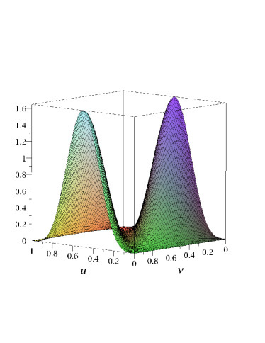
Figure 3: The plot shows ${\widetilde{\!\widetilde{f}}}_{k}$ as a function of $u:=h\tau_{1}/\bigl{[}4\delta\operatorname{atanh}(h/2)\bigr{]}$ and $v:=\tau_{2}/(2\delta)$ over the full period $0\leq u\leq 1$ and $0\leq v\leq 1$, for $s=0$ and $k=1$. Note the zeroes at $u\equiv 0\mod 1$ and at $u+v\equiv 0\mod 1$.

VII Conclusions

We have analysed the entanglement degradation for a massless Dirac field between two cavities in $(1+1)$-dimensional Minkowski spacetime, one cavity inertial and the other moving along a trajectory that consists of inertial and uniformly accelerated segments. Working in the approximation of small accelerations but arbitrarily long travel times, we found that the degradation is qualitatively similar to that found in bruschifuenteslouko11 for a massless scalar field with Dirichlet boundary conditions. The degradation is periodic in the durations of the individual inertial and accelerated segments, and we identified a travel scenario where the degradation caused by accelerated segments can be undone by fine-tuning the duration of an inertial segment. The presence of charge allows however a wider range of initial states of interest to be analysed. As an example, we identified a state where the entanglement degradation contains a contribution due to interference between excitations of opposite charge.

Compared with bosons, working in a fermionic Fock space led both to technical simplifications and to technical complications. A technical simplification was that the relevant reduced density matrices act in a lower-dimensional Hilbert space because of the fermionic statistics, and this made it possible to quantify the entanglement not just in terms of the negativity but also in terms of the CHSH inequality. It would further be possible to investigate the concurrence, although doing so would require pushing the perturbative low-acceleration expansion to a higher order than we have done in this paper.

A technical complication was that when the boundary conditions at the cavity walls were chosen in an arguably natural way that preserves charge conjugation symmetry, the spectrum contained a zero mode. This zero mode could not be consistently omitted by hand, but we were able to regularise the zero mode by treating the charge-symmetric boundary conditions as a limiting case of charge-nonsymmetric boundary conditions. All our entanglement measures remained manifestly well defined when the regulator was removed.

Another technical complication occurring for fermions is the ambiguity monteromartinmartinez11 in the choice of the basis of the two-fermion Hilbert space in (48). An alternative valid choice of basis is obtained by reversing the order of the single particle kets in (48), which amounts to a change of the signs in the off-diagonal elements of (48a) and (48b). While our treatment does not remove this ambiguity, all of our results for the entanglement and the nonlocality of these states are independent of the chosen convention.

Our analysis contained two significant limitations. First, while our Bogoliubov transformation technique can be applied to arbitrarily complicated graftings of inertial and uniformly accelerated cavity trajectory segments, the treatment is perturbative in the accelerations and hence valid only in the small acceleration limit. We were thus not able to address the large acceleration limit, in which striking qualitative differences between bosonic and fermionic entanglement have been found for field modes that are not confined in cavities fuentesschullermann05 ; alsingfuentesschullermanntessier06 ; bruschiloukomartinmartinezdraganfuentes10 ; martinmartinezfuentes11 ; friiskoehlermartinmartinezbertlmann11 .

Second, a massless fermion in a $(1+1)$-dimensional cavity is unlikely to be a good model for systems realisable in a laboratory. A fermion in a linearly-accelerated rectangular cavity in $(3+1)$ dimensions can be reduced to the $(1+1)$-dimensional case by separation of variables, but for generic field modes the transverse quantum numbers then contribute to the effective $(1+1)$-dimensional mass; further, any foreseeable experiment would presumably need to use fermions that have a positive mass already in $(3+1)$ dimensions before the reduction. It would be possible to analyse our $(1+1)$-dimensional system for a massive fermion, and we anticipate that the mass would enhance the magnitude of the entanglement degradation as in the bosonic situation bruschifuenteslouko11 . A detailed analysis of a massive fermion could become of experimental interest if guided by insights as to how a massive fermion might be confined to a cavity in a concrete laboratory setting.

We started this paper by emphasising that a cavity localises the quantum degrees of freedom in the worldtube of the cavity, and our assumption of inertial initial and final trajectory segments localises the acceleration effects in a finite interval of the cavity’s proper time. We should perhaps end by emphasising that we are not attempting to localise measurements of the field at more precise spacetime locations within the worldtube of the cavity, and we are hence not proposing cavities as a fundamental solution to the open conceptual issues of a quantum measurement theory in relativistic spacetime sorkin-impossible . A cavity can however reduce the measurement ambiguities from, say, megaparsecs to centimetres, which may well suffice to resolve the conceptual issues in specific experimental settings of interest, gedanken or otherwise.

References

• (1) P. M. Alsing and G. J. Milburn, Phys. Rev. Lett. 91, 180404 (2003).
• (2) I. Fuentes-Schuller and R. B. Mann, Phys. Rev. Lett. 95, 120404 (2005).
• (3) P. M. Alsing, I. Fuentes-Schuller, R. B. Mann and T. E. Tessier, Phys. Rev. A 74, 032326 (2006).
• (4) D. E. Bruschi, J. Louko, E. Martín-Martínez, A. Dragan and I. Fuentes, Phys. Rev. A 82, 042332 (2010).
• (5) E. Martín-Martínez and I. Fuentes, Phys. Rev. A 83, 052306 (2011).
• (6) N. Friis, P. Köhler, E. Martín-Martínez and R. A. Bertlmann, Phys. Rev. A 84, 062111 (2011).
• (7) E. Martín-Martínez, “Relativistic Quantum Information: developments in Quantum Information in general relativistic scenarios,” PhD Thesis, Complutense University of Madrid (2011) [arXiv:1106.0280 [quant-ph]].
• (8) W. G. Unruh, Phys. Rev.  D 14, 870 (1976).
• (9) R. M. Wald, Quantum field theory in curved spacetime and black hole thermodynamics (University of Chicago Press, Chicago, 1994).
• (10) D. E. Bruschi, I. Fuentes and J. Louko, e-print arXiv:1105.1875v3 [quant-ph] (2011).
• (11) J. F. Clauser, M. A. Horne, A. Shimony, and R. A. Holt, Phys. Rev. Lett. 23, 880 (1969).
• (12) R. Horodecki, P. Horodecki, and M. Horodecki, Phys. Lett. A 200, 340 (1995).
• (13) M. Srednicki, Quantum Field Theory (Cambridge University Press, Cambridge, England, 2007).
• (14) M. Reed and M. Simon, Methods of Modern Mathematical Physics, (Academic Press, New York, 1975), Vol. 2.
• (15) G. Bonneau, J. Faraut and G. Valent, Am. J. Phys. 69, 322 (2001).
• (16) N. D. Birrell and P. C. W. Davies, Quantum Fields in Curved Space (Cambridge University Press, Cambridge, England, 1982).
• (17) D. McMahon, P. M. Alsing and P. Embid, eprint arXiv:gr-qc/0601010v2 (2006).
• (18) A. Fabbri and J. Navarro-Salas, Modeling Black Hole Evaporation (Imperial College Press, London, 2005).
• (19) M. Montero and E. Martín-Martínez, Phys. Rev. A 83, 062323 (2011).
• (20) G. Vidal, and R. F. Werner, Phys. Rev. A 65, 032314 (2002).
• (21) K. Audenaert, M. B. Plenio and J. Eisert, Phys. Rev. Lett. 90, 027901 (2003).
• (22) M. B. Plenio and S. Virmani, Quant. Inf. Comput. 7, 1 (2007).
• (23) M. Horodecki, P. Horodecki, and R. Horodecki, Phys. Rev. Lett. 80, 5239 (1998).
• (24) Digital Library of Mathematical Functions (National Institute of Standards and Technology, 2010), http://dlmf.nist.gov/.
• (25) W. K. Wootters, Phys. Rev. Lett. 80, 2245 (1998).
• (26) A. Smith and R. B. Mann, eprint arXiv:1107.4633v1 [quant-ph] (2011).
• (27) R. D. Sorkin, in: Directions in General Relativity: Proceedings of the 1993 International Symposium, College Park,Maryland, 1993, edited by B.-L. Hu and T. A. Jacobson (Cambridge University Press, Cambridge, England, 1993), Vol. 2, p. 293, [arXiv:gr-qc/9302018v2].