Superfluidity of dipole excitons in two layers of gapped graphene

Abstract

A study of the formation of excitons as a problem of two Dirac particles confined in two-layer graphene sheets separated by a dielectric when gaps are opened and they interact via a Coulomb potential is presented. We propose to observe Bose-Einstein condensation and superfluidity of quasi-two-dimensional dipole excitons in double layer graphene in the presence of band gaps. The energy spectrum of the collective excitations, the sound spectrum, and the effective exciton mass are functions of the energy gaps, density and interlayer separation. The superfluid density $n_{s}$ and temperature of the Kosterlitz-Thouless phase transition $T_{c}$ are decreasing functions of the energy gaps as well as the interlayer separation, and therefore, could be controlled by these parameters.

I Introduction

The many-particle systems of the spatially-indirect dipole excitons in coupled quantum wells (CQW’s) have been the subject of recent experimental investigations Snoke ; Butov ; Timofeev ; Eisenstein . These systems are of interest, in particular, in connection with the possibility of Bose-Einstein condensation (BEC) and superfluidity of dipole excitons or electron-hole pairs, which would manifest itself in the CQW’s as persistent electrical currents in each well and also through coherent optical properties and Josephson phenomena Lozovik ; Littlewood ; Vignale ; Berman .

Recent technological advances have allowed the production of graphene, which is a 2D honeycomb lattice of carbon atoms that form the basic planar structure in graphite Novoselov1 ; Zhang1 . Graphene has been attracting a great deal of experimental and theoretical attention because of its unusual properties in its band structure Novoselov2 ; Zhang2 ; Nomura ; Jain . It is a gapless semiconductor with massless electrons and holes which have been described as Dirac-fermions DasSarma . Due to the absence of a gap between the conduction and valence bands in graphene, the screening effects result in the absence of excitons in graphene. However, the gap in the electron spectrum in graphene can be opened by applying the magnetic field, which results in the formation of magnetoexcitons iyengar07 . The BEC and superfluidity of spatially-indirect magnetoexcitons with spatially separated electrons and holes in high magnetic field have been studied in graphene double layer Berman_L_G and graphene superlattice Berman_K_L ; Berman_K_L_2 . The electron-hole pair condensation in the graphene-based bilayers have been studied in [Sokolik, ; MacDonald1, ; MacDonald2, ; Efetov, ]. However, the effective mass of magnetoexcitons increases when the magnetic field increases and, therefore, the Kosterlitz-Thouless critical temperature of the superfluidity decreases with increasing magnetic field.

In this paper we propose a new physical realization of an excitonic BEC and superfluidity in two parallel graphene layers, when one layer is filled by electrons, and the other one is filled by holes. We consider two parallel graphene layers separated by an insulating slab (e.g. $SiO_{2}$) and propose the formation of the excitons due to the gap opening in the electron and hole spectra in the two graphene layers. The advantage of the consideration of exciton formed by an electron and a hole from two different graphene layers, separated by an insulating slab, is that the dielectric slab creates the barrier for the electron-hole recombination which increases the life-time of the exciton compared to the exciton formed by an electron and a hole in a single graphene layer.

There are different mechanisms of the band gap opening in graphene. Substrate-induced band gap opening in epitaxial graphene is caused by the breaking of sublattice symmetry owing to the graphene substrate interaction Zhou . When graphene is epitaxially grown on SiC substrate, a gap of $\sim 0.26\ \mathrm{eV}$ is produced Zhou . The electronic structure of graphene can be tuned by an organic molecule. The band gap can be opened in graphene due to the charge transfer between an organic molecule and graphene Lu . It was demonstrated by angle-resolved photoemission spectroscopy that a tunable gap in quasi-free-standing monolayer graphene on Au can be induced by hydrogenation Haberer . The size of the gap can be controlled by hydrogen loading and reaches $\sim 1.0\ \mathrm{eV}$ for a hydrogen coverage of $8\mathrm{\%}$ Haberer . The band gap tuning in hydrogenated graphene was also analyzed within the density functional theory Gao .

The equilibrium system of local pairs of spatially separated electrons and holes can be created by varying the chemical potential, using a bias voltage between two graphene layers or between two gates located near the corresponding graphene sheets. For simplicity, we also call these equilibrium local electron-hole pairs as indirect excitons. Excitons with spatially separated electrons and holes can be created also by laser pumping (far infrared in graphene) and by applying perpendicular electric field as for the CQW’s Snoke ; Butov ; Eisenstein . We assume that the system is in a quasi-equilibrium state. Below we study the low-density regime for excitons, i.e. exciton radius $a<n^{-1/2}$, where $n$ is the 2D exciton density. In this system the effective exciton mass can be controlled by the gap. The effective exciton mass can be small relative to the mass of free electron, and the Kosterlitz-Thouless transition temperature $T_{c}$ controlled by the gap is expected to be the same order or relatively high compared to the coupled quantum wells case.

Our paper is organized in the following way. In Sec. II we present the Hamiltonian of the spatially separated electron and hole in two different parallel graphene sheets separated by a dielectric in the presence of the band gap. In Sec. III we obtain the single-particle energy spectrum of dipole excitons in two-layers graphene and find the effective exciton mass. In Sec. IV we obtain the spectrum of collective excitation in the weakly-interacting gas of dipole excitons. The density of the superfluid component and the temperature of the phase transitions for the system of dipole excitons in two-layer graphene in the presence of a band gap are obtained in Sec. V. Finally, the discussion of the results and conclusions follow in Sec. VI.

II Exciton Hamiltonian

Let us consider a system of electrons and holes located in two different parallel graphene sheets. In this system electrons and holes move in two separate sheets with honeycomb lattice structure. We assume that excitons in this system are formed by the electrons located in the one graphene sheet and, correspondingly, the holes located in the other. Since the motion of the electron is restricted in one graphene sheet and the motion of the hole is restricted in the other graphene sheet, we replace the coordinate vectors of the electron and hole by their projections $\mathbf{r}_{1}$ and $\mathbf{r}_{2}$ on plane of one of the graphene sheet. These new in-plane coordinates $\mathbf{r}_{1}$ and $\mathbf{r}_{2}$ will be used everywhere below in our paper. Thus, we reduced the restricted 3D two-body problem to the 2D two-body problem on the graphene plane. Each honeycomb lattice is characterized by the coordinates $(\mathbf{r}_{j},1)$ on sublattice A and $(\mathbf{r}_{j},2)$ on sublattice B with $j=1,2$ referring to the two sheets. Then the two-particle wavefunction, describing two particles in different sheets, reads $\Psi(\mathbf{r}_{1},s_{1};\mathbf{r}_{2},s_{2})$, where $\mathbf{r}_{1}$ and $\mathbf{r}_{2}$ represent the coordinates of the electron and hole, correspondingly, and $s_{1}$, $s_{2}$ are sublattice indices. This wavefunction can also be understood as a four-component spinor, where the spinor components refer to the four possible values of the sublattice indices $s_{1},s_{2}$;

$$\Psi(\mathbf{r}_{1},s_{1};\mathbf{r}_{2},s_{2})=\left({\begin{array}[]{c}\phi_{aa}(\mathbf{r}_{1},\mathbf{r}_{2})\\ \phi_{ab}(\mathbf{r}_{1},\mathbf{r}_{2})\\ \phi_{ba}(\mathbf{r}_{1},\mathbf{r}_{2})\\ \phi_{bb}(\mathbf{r}_{1},\mathbf{r}_{2})\end{array}}\right)\ .$$ (1)

In other words, the spinor components are from the same tight-binding wavefunction at different sites. Each graphene sheet has an energy gap. Obviously the gaps in these sheets are independent and in the general case we can introduce two non-equal gaps $\delta_{1}$ and $\delta_{2}$, corresponding to the first and the second graphene sheet, respectively. The gap parameters $\delta_{1}$, $\delta_{2}$ are the consequence of adatoms on the graphene sheets, which create a one-particle potential.

The corresponding hopping matrix for two non-interacting particles, including the energy gaps $\delta_{1}$ and $\delta_{2}$ on the first and second sheets, correspondingly, then reads

$$\mathcal{H}_{0}=\left(\begin{array}[]{cccc}-\delta_{1}+\delta_{2}&d_{2}&d_{1}&0\\ d_{2}^{{\dagger}}&-\delta_{1}-\delta_{2}&0&d_{1}\\ d_{1}^{{\dagger}}&0&\delta_{1}+\delta_{2}&d_{2}\\ 0&d_{1}^{{\dagger}}&d_{2}^{{\dagger}}&\delta_{1}-\delta_{2}\end{array}\right)\ ,$$ (2)

In Eq. (2) $d_{1}=\hbar v_{F}(-i\frac{\partial}{\partial x_{1}}-\frac{\partial}{\partial y_{1}})$, $d_{2}=\hbar v_{F}(-i\frac{\partial}{\partial x_{2}}-\frac{\partial}{\partial y_{2}})$ and the corresponding hermitian conjugates are $d_{1}^{{\dagger}}=\hbar v_{F}(-i\frac{\partial}{\partial x_{1}}+\frac{\partial}{\partial y_{1}})$, $d_{2}^{{\dagger}}=\hbar v_{F}(-i\frac{\partial}{\partial x_{2}}+\frac{\partial}{\partial y_{2}})$, where $x_{1}$, $y_{1}$ and $x_{2}$, $y_{2}$ are the coordinates of vectors $\mathbf{r}_{1}$ and $\mathbf{r}_{2}$, correspondingly, $v_{F}=\sqrt{3}at/(2\hbar)$ is the Fermi velocity of electrons in graphene, where $a=2.566\ \mathrm{\AA}$ is a lattice constant and $t\approx 2.71\ \mathrm{eV}$ is the overlap integral between the nearest carbon atoms  Lukose . This Hamiltonian allows us to write the eigenvalue equation for two non-interacting particles as

$$\mathcal{H}_{0}\mathit{\Psi}_{0}=\epsilon_{0}\mathit{\Psi}_{0}\ ,$$ (3)

which leads to the following eigenenergies:

$$\epsilon_{0}(k_{1},\delta_{1};k_{2},\delta_{2})=\pm\sqrt{k_{1}^{2}+k_{2}^{2}+\delta_{1}^{2}+\delta_{2}^{2}\pm 2\sqrt{(k_{1}^{2}+\delta_{1}^{2})(k_{2}^{2}+\delta_{2}^{2})}}=\pm\sqrt{k_{1}^{2}+\delta_{1}^{2}}\pm\sqrt{k_{2}^{2}+\delta_{2}^{2}}\ .$$ (4)

where $k_{1}$ and $k_{2}$ are momentum of each particle, correspondingly. Eq. (4) gives the energy spectrum for two non-interacting particles in the presents of the non-equal gaps energies $\delta_{1}$ and $\delta_{2}$. The energy dispersion is symmetrical with respect to the replacement of particles $1$ and $2$. When there are no gaps, $\delta_{1}=0$ and $\delta_{2}=0$, as it follows from (4) the energy dispersion is  $\pm k_{1}\pm k_{2}$.

Let’s now consider the electron and hole located in two graphene sheets with the interlayer separation $D$, and interacting via the Coulomb potential $V(r)=-e^{2}/\varepsilon\sqrt{r^{2}+D^{2}}$ where $r$ is the projection of the distance between an electron and a hole on the plane parallel to the graphene sheets, $e$ is the electron charge, and $\epsilon$ is the dielectric constant of the dielectric between graphene sheets. Now the problem for the two interacting particles located in different graphene sheets with the broken sublattice symmetry in each sheet can be described by the Hamiltonian

$$\mathcal{H}=\left(\begin{array}[]{cccc}-\delta_{1}+\delta_{2}+V(r)&d_{2}&d_{1}&0\\ d_{2}^{{\dagger}}&-\delta_{1}-\delta_{2}+V(r)&0&d_{1}\\ d_{1}^{{\dagger}}&0&\delta_{1}+\delta_{2}+V(r)&d_{2}\\ 0&d_{1}^{{\dagger}}&d_{2}^{{\dagger}}&\delta_{1}-\delta_{2}+V(r)\end{array}\right)\ ,$$ (5)

and the eigenvalue problem for Hamiltonian (5) is

$$\mathcal{H}\Psi=\epsilon\Psi$$ (6)

where $\Psi$ are four-component eigenfunctions as given in Eq.(1).

The Hamiltonian (5) describes two interacting particles located in two graphene sheets and satisfies the following conditions:

i) when the interaction between particles vanished $V(r)=0$ it describes two independent particles, each located in the separate graphene sheet, having two independent gaps energies related to the broken sublattice symmetry in each graphene sheet.

ii) when the gaps in each graphene sheet vanish, $\delta_{1}=0$ and $\delta_{2}=0$ the Hamiltonian describes two interacting particles in one graphene sheet Sabio (let us mention that for $\delta_{1}=\delta_{2}=0$ and $D=0$ the Hamiltonian (5) is identical to the Hamiltonian $(2)$ in Ref. Sabio representing the two-particle problem in one graphene graphene sheet if the band gap is absent) if a two-body potential is $e^{2}/\varepsilon r$ or in two graphene sheets with the interlayer separation $D$, and interacting via the potential $V(r)=-e^{2}/\varepsilon\sqrt{r^{2}+D^{2}}$.

iii) when both gaps vanish $\delta_{1}=0$ and $\delta_{2}=0$, as well as two-body potential $V(r)=0$, the Hamiltonian describes two non-interacting Dirac particles. It is important to mentioned that eigenenergies are symmetrical with respect of replacement particle $1$ and $2$.

In Hamiltonian (5) the center-of-mass energy can not be separated from the relative motion even though the interaction $V=V(r)$ depends only on the coordinate of the relative motion. This is caused by the chiral nature of Dirac electron in graphene. The similar conclusion was made for the two-particle problem in graphene in Ref. [Sabio, ], where two particles in a single sheet were considered without gaps and $D=0$.

III single exciton eigenvalue problem

Since the electron-hole Coulomb interaction depends only on the relative coordinate, we introduce the new “center-of-mass” coordinates in the plane of a graphene sheet $(x,y)$:

$$\mathbf{R}=\alpha\mathbf{r}_{1}+\beta\mathbf{r}_{2}\ ,$$

$$\mathbf{r}=\mathbf{r}_{1}-\mathbf{r}_{2}\ .$$ (7)

Here the coefficients $\alpha$ and $\beta$ are to be determined later. Apparently we can use the analogy of the two-particle problem for gapped Dirac particles in two-layer graphene with the center-of-mass coordinates for the case of Schrödinger equation. The coefficients $\alpha$ and $\beta$ will be found below from the condition of the separation of the coordinates of the center-of-mass and relative motion in the Hamiltonian in the one-dimensional “scalar” equation determining the corresponding component of the wave function.

We are looking for the solution of (5) in the form

$$\Psi_{j}(\mathbf{R},\mathbf{r})=\texttt{e}^{i\mathbf{\mathcal{K}}\cdot\mathbf{R}}\psi_{j}(\mathbf{r})\ .$$ (8)

Let’s introduce the following notations:

$$\mathcal{K}_{+}=\mathcal{K}\texttt{e}^{i\Theta}=\mathcal{K}_{x}+i\mathcal{K}_{y}\ ,$$

$$\mathcal{K}_{-}=\mathcal{K}\texttt{e}^{-i\Theta}=\mathcal{K}_{x}-i\mathcal{K}_{y}\ ,$$

$$\Theta=\tan^{-1}\left({\frac{\mathcal{K}_{y}}{\mathcal{K}_{x}}}\right)\ ,$$ (9)

and rewrite the Hamiltonian (5) in a form of the $2\times 2$ matrix as

$$\mathcal{H}=\left({\begin{array}[]{cc}\mathcal{O}_{2}+V(r)\sigma_{0}-\delta_{1}\sigma_{0}+\delta_{2}\sigma_{3}&\mathcal{O}_{1}\\ \mathcal{O}_{1}^{{\dagger}}&\mathcal{O}_{2}+V(r)\sigma_{0}-\delta_{1}\sigma_{0}+\delta_{2}\sigma_{3}\end{array}}\right)\ ,$$ (10)

where $\mathcal{O}_{1}$ and $\mathcal{O}_{2}$ are given by

$$\mathcal{O}_{1}=\hbar v_{F}\left({\alpha\mathcal{K}_{-}-i\partial_{x}-\partial_{y}}\right)\sigma_{0}=\hbar v_{F}\alpha\mathcal{K}_{-}\sigma_{0}-\hbar v_{F}(i\partial_{x}+\partial_{y})\sigma_{0},$$ (11)

$$\mathcal{O}_{2}=\hbar v_{F}\left({\begin{array}[]{cc}0&\beta\mathcal{K}_{-}+i\partial_{x}+\partial_{y}\\ \beta\mathcal{K}_{+}+i\partial_{x}-\partial_{y}&0\end{array}}\right)=$$ (14)

$$\hbar v_{F}\beta\left({\begin{array}[]{cc}0&\mathcal{K}_{x}-i\mathcal{K}_{y}\\ \mathcal{K}_{x}+i\mathcal{K}_{y}&0\end{array}}\right)+\left({\begin{array}[]{cc}0&i\partial_{x}+\partial_{y}\\ i\partial_{x}-\partial_{y}&0\end{array}}\right)\ ,$$ (19)

where $x$ and $y$ are the components of vector $\mathbf{r}$, $\sigma_{j}$ are the Pauli matrices, $\sigma_{0}$ is the $2\times 2$ unit matrix, also $\partial_{x}=\partial/\partial x$ and $\partial_{y}=\partial/\partial y$. Analysis of the operators (11) and (19) shows that the coordinates of the center-of-mass and relative motion can be separated.

For $\phi_{aa}$ we can rewrite the eigenvalue problem as a one-dimensional equation (see Appendix A):

$$\left({\frac{(\hbar v_{F}\mathcal{K})^{2}}{2\epsilon}+V(r)-\frac{\epsilon(\hbar v_{F})^{2}\nabla_{\mathbf{r}}^{2}}{2\left({\epsilon^{2}-(\delta_{1}+\delta_{2})^{2}}\right)}}\right)\phi_{aa}=\left[{\epsilon+\delta_{1}-\delta_{2}}\right]\phi_{aa}\ .$$ (20)

The other components of (1) are given as:

$$\Psi_{b}=-(\epsilon\sigma_{0}-iD_{2}-\delta_{1}\sigma_{0}-\delta_{2}\sigma_{3}-V(r)\sigma_{0})^{-1}iD_{1}^{\dagger}\Psi_{a}$$ (21)

for

$$\Psi_{a}=\left({\begin{array}[]{c}\phi_{aa}\\ \phi_{ab}\end{array}}\right),\ \ \ \Psi_{b}=\left({\begin{array}[]{c}\phi_{ba}\\ \phi_{bb}\end{array}}\right)$$ (22)

and

$$D_{1}=\left({\begin{array}[]{cc}\partial_{x_{1}}-i\partial_{y_{1}}&0\\ 0&\partial_{x_{1}}-i\partial_{y_{1}}\\ \end{array}}\right)=(\partial_{x_{1}}-i\partial_{y_{1}})\sigma_{0}$$ (23)

$$D_{2}=\left({\begin{array}[]{cc}0&\partial_{x_{2}}-i\partial_{y_{2}}\\ \partial_{x_{2}}+i\partial_{y_{2}}&0\\ \end{array}}\right)=\partial_{x_{2}}\sigma_{1}+\partial_{y_{2}}\sigma_{2}$$ (24)

with Pauli matrices $\sigma_{j}$ and $2\times 2$ unit matrix $\sigma_{0}$. Moreover, we have

$$\phi_{ab}=\left[\epsilon+\delta_{1}+\delta_{2}-V(r)+\frac{1}{\epsilon-\delta_{1}+\delta_{2}}(\partial_{x_{1}}^{2}+\partial_{y_{1}}^{2})\right]^{-1}(i\partial_{x_{2}}-\partial_{y_{2}})\phi_{aa}\ .$$ (25)

Assuming $r\ll D$ and substituting the second-order series expansion for the interaction potential $V(r)=-V_{0}+\gamma r^{2}$ into Eq. (20), where $V_{0}=e^{2}/(\varepsilon D)$ and $\gamma=e^{2}/(2\varepsilon D^{3})$, we obtain

$$\left({-\frac{\epsilon(\hbar v_{F})^{2}\nabla_{\mathbf{r}}^{2}}{2\left({\epsilon^{2}-(\delta_{1}+\delta_{2})^{2}}\right)}+\gamma r^{2}}\right)\phi_{aa}=\left[{\epsilon+\delta_{1}-\delta_{2}+V_{0}-\frac{(\hbar v_{F}\mathcal{K})^{2}}{2\epsilon}}\right]\phi_{aa}\ .$$ (26)

The last equation can be rewritten in the form of the two-dimensional isotropic harmonic oscillator:

$$\left({-\mathcal{F}_{1}(\epsilon)\nabla_{\mathbf{r}}^{2}+\gamma r^{2}}\right)\phi_{aa}=\mathcal{F}_{0}(\epsilon)\phi_{aa}\ ,$$ (27)

where

$$\mathcal{F}_{1}=\frac{\epsilon(\hbar v_{F})^{2}}{2\left({\epsilon^{2}-(\delta_{1}+\delta_{2})^{2}}\right)}\ ,$$

$$\mathcal{F}_{0}=\epsilon+\delta_{1}-\delta_{2}+V_{0}-\frac{(\hbar v_{F}\mathcal{K})^{2}}{2\epsilon}\ .$$ (28)

The solution of Eq. (27) is well known (see, for example, Ref. arfken85 ) and is given by

$$\frac{\mathcal{F}_{0}(\epsilon)}{\mathcal{F}_{1}(\epsilon)}=2N\sqrt{\frac{\gamma}{\mathcal{F}_{1}(\epsilon)}}\ ,$$ (29)

where $N=2n_{1}+n_{2}+1$ with $n_{1}=0,1,2,3,\ldots$, $n_{2}=0,\pm 1,\pm 2,\pm 3,\ldots,\pm n_{1}$ are the quantum numbers of the 2D harmonic oscillator.

After some straightforward but lengthy calculations (cf Appendix B) we obtain the following expression for the energy in quadratic order with respect to $\mathcal{K}$

$$\epsilon=-V_{0}+\sqrt{\mu^{2}+\frac{C_{1}}{\mu}}+\frac{1}{2\mu^{4}}\frac{C_{1}}{\sqrt{1+\frac{C_{1}}{\mu^{3}}}}(\hbar v_{F}\mathcal{K})^{2}\ ,$$ (30)

where $\mu=\delta_{1}+\delta_{2}$ and $C_{1}=2\gamma N^{2}(\hbar v_{F})^{2}$. Thus, from (30) we can conclude that the effective exciton mass $M$ is given as a function of total energy gap $\delta_{1}+\delta_{2}$ and the parameter $C_{1}\propto D^{-3}$ as

$$M=\frac{\mu^{4}}{v_{F}^{2}C_{1}}\sqrt{1+\frac{C_{1}}{\mu^{3}}}\ .$$ (31)

The effective exciton mass $M$ as a function of total energy gap $\delta_{1}+\delta_{2}$ and the interlayer separation D defined by Eq.(31) is plotted in Fig. 1. According to Fig. 1, the effective exciton mass $M$ increases when the total energy gap $\delta_{1}+\delta_{2}$ and the interlayer separation $D$ increase. The three-dimensional Fig. 1$c)$ demonstrates dependence of the effective exciton mass on the total energy gap and interlayer separation. The dependence of the effective exciton mass $M$ on the interlayer separation $D$ is caused by the quasi-relativistic Dirac Hamiltonian of the gapped electrons and holes in graphene layers. Let us mention that for the excitons in CQW s the effective exciton mass does not depend on the interlayer separation, because the electrons and holes in CQW s are described by a Schrödinger Hamiltonian, while excitons in two graphene layers are described by the Dirac-like Hamiltonian (5).

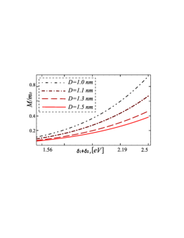
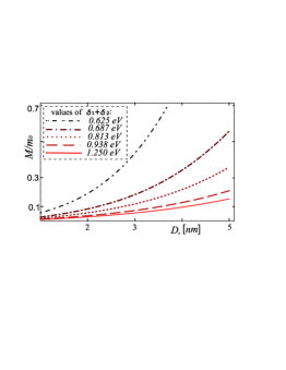
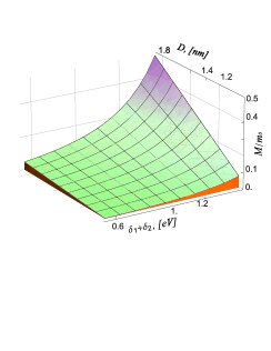
Figure 1: The effective exciton mass $M$ in the units of free electron mass $m_{0}$ as a function of the total energy gap for the different graphene interlayer separations $D$ (a), as the function of on interlayer separation $D$ for different values of the total energy gap (b) and as the function of the total energy gap and graphene interlayer separation (c).

IV Collective properties of dipole excitons in a two-layer graphene

After having found the mass and the energy for a single exciton in the separated double layer of graphene, we turn now to an ensemble of excitons in this structure. Due to interlayer separation $D$ indirect excitons both in ground state ($n_{1}=n_{2}=0$) and in excited states have non-zero electrical dipole moments. We assume that indirect exciton interact as parallel dipoles. This is valid when $D$ is larger than the mean separation $\langle r\rangle$ between electron and hole along graphene layers $D\gg\langle r\rangle$.

The distinction between exciton and bosons manifests itself in exchange effects Halperin_Rice ; KelKoz ; Berman ; Berman_Willander . These effects for exciton with spatially separated electron and hole in a dilute system $na^{2}\ll 1$ ($n\ll D^{-2}$) are suppressed due to the negligible overlapping of wave functions of two exciton in the presence of the potential barrier, associated with the dipole-dipole repulsion of an indirect exciton Berman . Two indirect exciton in a dilute system interact as $U(R)=e^{2}D^{2}/(\varepsilon R^{3})$, where $R$ is the distance between exciton dipoles along the graphene layers. A small tunneling parameter $t$ due to this barrier is Berman_L_G :

$$t=\exp\left[-\frac{1}{\hbar}\int_{a}^{r_{0}}\sqrt{2M\left(\frac{e^{2}D^{2}}{\varepsilon R^{3}}-\frac{\kappa^{2}}{2M}\right)}\ dR\right],$$

where

$$\kappa^{2}=\frac{2\pi\hbar^{2}n}{s\log\left(s\hbar^{4}\varepsilon^{2}/(2\pi nM^{2}e^{4}D^{4})\right)}$$

is the characteristic value of the center-of-mass exciton momentum $\hbar\mathcal{K}$ defined as $\kappa=\sqrt{2M\mu_{ex}}$, where $\mu_{ex}$ is the chemical potential of the system (see below). In Eq. (IV), $r_{0}=(2Me^{2}D^{2}/\kappa^{2})^{1/3}$ is the classical turning point for the dipole-dipole interaction, $s=4$ is the spin degeneracy factor for the excitons and $M$ is the effective exciton mass in the ground state given by Eq. (31). Then the small tunneling parameter $t$ has the form $t\sim\exp[-2\hbar^{-1}(M)^{1/2}eDa^{-1/2}]$. Therefore, we neglect the overlap of the exciton wavefunctions in the limit of large layer separation $D$ and consider the gas of excitons as a Bose gas. Consequently, at sufficiently low temperatures the dilute gas of excitons forms a Bose-Einstein condensate Abrikosov ; Griffin . Formally, the exciton gas can be treated by the conventional diagram technique for a boson system. In particular, the effective interaction of the dilute two-dimensional exciton gas (at $na^{2}\ll 1$) can be described by a summation of ladder diagrams Abrikosov . From the latter we obtain an integral equation for vertex function $\Gamma$, depending on three momenta $\mathbf{p},\mathbf{p}^{\prime},\mathbf{P}$ and the frequency $\Omega$, as

$$\Gamma(\mathbf{p},\mathbf{p}^{\prime};\mathbf{P},\Omega)=U(\mathbf{p}-\mathbf{p}^{\prime})+s\int\frac{d^{2}q}{(2\pi\hbar)^{2}}\frac{U(\mathbf{p}-\mathbf{q})\Gamma(\mathbf{q},\mathbf{p}^{\prime};\mathbf{P},\Omega)}{\frac{\mathcal{L}^{2}}{M}+\Omega-\frac{\mathbf{P}^{2}}{4M}-\frac{q^{2}}{M}+i\delta^{\prime}}\hskip 14.22636pt(\delta^{\prime}\rightarrow+0)\ ,$$ (32)

where $U(\mathbf{p}-\mathbf{p}^{\prime})$ is a dipole-dipole interaction in momentum representation. This equation is also represented by diagrams in Fig. 2. The chemical potential of the system is given by

$$\mu_{ex}=\frac{\kappa^{2}}{2M}=n_{0}\Gamma(0,0;0,0)\equiv n_{0}\Gamma_{0}\ .$$ (33)

Equation (32) can be solved easily when the excitons occupy the ground state $n_{1}=n_{2}=0$. Then the energy spectrum of the exciton is given by $\epsilon(P)=P^{2}/(2M)$, where the mass $M$ is given by Eq. (31).

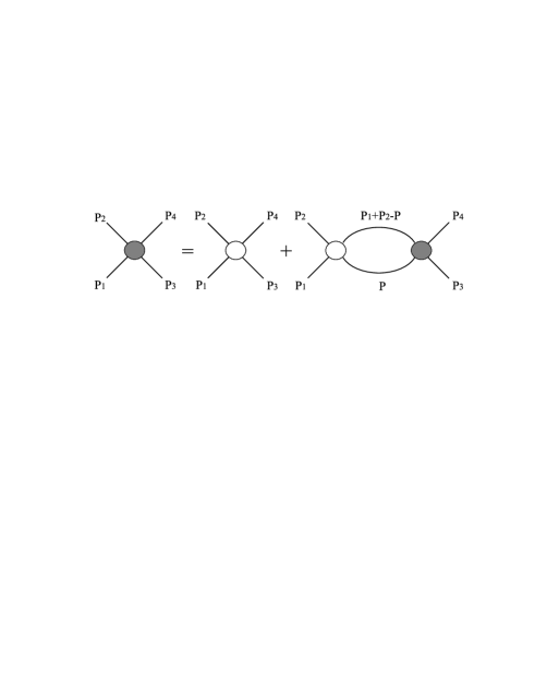
Figure 2: The equation for the vertex $\Gamma$ in momentum representation

The specific feature of a two-dimensional Bose system is connected with the logarithmic divergence of two-dimensional scattering amplitude at zero energy Berman ; Berman_Willander ; Yudson . A simple analytical solution of Eq. (32) for the chemical potential can be obtained if $\kappa Me^{2}D^{2}/(\hbar^{3}\varepsilon)\ll 1$, which gives for the chemical potential $\mu_{ex}$

$$\mu_{ex}=\frac{\kappa^{2}}{2M}=\frac{\pi\hbar^{2}n}{sM\log\left[s\hbar^{4}\varepsilon^{2}/\left(2\pi nM^{2}e^{4}D^{4}\right)\right]}\ .$$ (34)

The solution of Eq. (32) at small momenta provides the sound spectrum of collective excitations $\epsilon(P)=c_{s}P$ with the sound velocity $c_{s}=\sqrt{\Gamma_{0}n/(4sM)}=\sqrt{\mu_{ex}/M}$. The appearance of a sound spectrum is a consequence of the dipole-dipole repulsion. This sound spectrum of the collective excitations reflects the possibility for the existence of an excitonic superfluidity at low temperatures in a double layer graphene, provided that the sound spectrum satisfies to the Landau criterion of superfluidity Abrikosov ; Griffin .

V Superfluidity of dipole excitons in double layer graphene

The dilute exciton gas which was discussed the previous section, consisting of electron-hole pairs on the graphene double layer, forms a collective state whose excitations are sound-like modes. This might be true at low temperatures, whereas at higher temperatures phase fluctuations can destroy this 2D collective state by creating vortex-like excitations (i.e. by unbinding vortex-antivortex pairs). The latter have short-range correlations which prevent a superfluid state. Therefore, superfluidity is only possible for temperatures below a critical temperature $T_{c}$. This critical temperature describes a Kosterlitz-Thouless transition Kosterlitz and is defined as

$$T_{c}=\frac{\pi\hbar^{2}n_{s}(T_{c})}{2k_{B}M}\ ,$$ (35)

where $n_{s}(T)$ is the superfluid density of the exciton system at the temperature $T$, and $k_{B}$ is Boltzmann constant.

The function $n_{s}(T)$ in (35) can be found from the relation $n_{s}=n-n_{n}$, where $n$ is the total density and $n_{n}$ is the normal component density. We determine the normal component density following the usual procedure Abrikosov . Suppose that the exciton system moves with a velocity $\mathbf{u}$. At nonzero temperatures $T$ dissipating quasiparticles will appear in this system. Since their density is small at low temperatures, one can assume that the gas of quasiparticles is an ideal Bose gas. To calculate the superfluid component density we find the total current of quasiparticles in a frame in which the superfluid component is at rest. Then we obtain the mean total current of 2D excitons in the coordinate system, moving with a velocity ${\bf u}$:

$$\left\langle\mathbf{J}\right\rangle=\frac{1}{M}\left\langle\mathbf{P}\right\rangle=\frac{s}{M}\int\frac{d\mathbf{P}}{(2\pi\hbar)^{2}}\mathbf{P}f\left(\epsilon(P)-\mathbf{P}\mathbf{u}\right)\ ,$$ (36)

where $f\left(\epsilon(P)\right)=\left(\exp\left[\epsilon(P)/(k_{B}T)\right]-1\right)^{-1}$ is the Bose-Einstein distribution function. Expanding the expression inside the integral and leaving the first order by $\mathbf{P}\mathbf{u}/(k_{B}T)$, we have:

$$\langle\mathbf{J}\rangle=-s\frac{\mathbf{u}}{2M}\int\frac{d\mathbf{P}}{(2\pi\hbar)^{2}}P^{2}\frac{\partial f\left(\epsilon(P)\right)}{\partial\epsilon}=\frac{3\zeta(3)s}{2\pi\hbar^{2}}\frac{k_{B}^{3}T^{3}}{Mc_{s}^{4}}\mathbf{u}\ ,$$ (37)

where $\zeta(z)$ is the Riemann zeta function ($\zeta(3)\simeq 1.202$). Then we define the normal component density $n_{n}$ as Abrikosov

$$\langle\mathbf{J}\rangle=n_{n}\mathbf{u}\ .$$ (38)

Comparing Eqs. (38) and (37), we obtain the expression for the normal density $n_{n}$, which implies for the superfluid density

$$n_{s}=n-\frac{3\zeta(3)}{2\pi\hbar^{2}}\frac{k_{B}^{3}T^{3}}{c_{s}^{4}M}\ .$$ (39)

It should be noticed that the expression for the superfluid density $n_{s}$ of the dilute exciton gas in the double layer graphene in the presence of the band gaps differs from the corresponding expression in semiconductor coupled quantum wells (compare with Refs. [Berman, ; Berman_Willander, ] by replacing the total exciton mass $M=m_{e}+m_{h}$ with the effective exciton mass $M$ given by Eq. (31)).

Using Eq. (39) for the density $n_{s}$ of the superfluid component, we obtain an equation for the Kosterlitz-Thouless transition temperature $T_{c}$. Its solution is

$$T_{c}=\left[\left(1+\sqrt{\frac{32}{27}\left(\frac{sMk_{B}T_{c}^{0}}{\pi\hbar^{2}n}\right)^{3}+1}\right)^{1/3}-\left(\sqrt{\frac{32}{27}\left(\frac{sMk_{B}T_{c}^{0}}{\pi\hbar^{2}n}\right)^{3}+1}-1\right)^{1/3}\right]\frac{T_{c}^{0}}{2^{1/3}}\ ,$$ (40)

where $T_{c}^{0}$ is the temperature at which the superfluid density vanishes in the mean-field approximation (i.e., $n_{s}(T_{c}^{0})=0$),

$$T_{c}^{0}=\frac{1}{k_{B}}\left(\frac{\pi\hbar^{2}nc_{s}^{4}M}{6s\zeta(3)}\right)^{1/3}\ .$$ (41)

The behavior of the Kosterlitz-Thouless transition temperature $T_{c}$ as a function of the total energy gap, exciton concentration $n$ and the interlayer separation $D$ is presented in Fig. 3, using Eqs. (40) and (41). As we can see in Fig. 3, $T_{c}$ increases when the exciton concentration $n$ and increases and decreases when total energy gap and and interlayer separation increaseincreases.

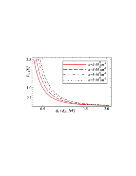
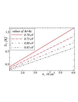
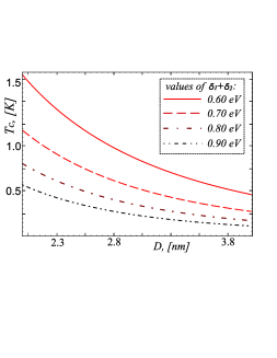
Figure 3: Kosterlitz-Thouless transition temperature $T_{c}$ as a function of the total energy gap $\delta_{1}+\delta_{2}$, exciton concentration $n$ and the separation between the two graphene layers: (a) demonstrates how the transition temperature depends on the total energy gap $\delta_{1}+\delta_{2}$ for the four different values of exciton mass concentration : $n=3.0\cdot 10^{11}cm^{-2};\;4.0\cdot 10^{11}cm^{-2};\;5.0\cdot 10^{11}cm^{-2};\;6.0\cdot 10^{11}cm^{-2}$; (b) shows the transition temperature dependence on the exciton concentration for ten different values of the total enertgy gap: $(\delta_{1}+\delta_{2}=0.70eV;\;0.75eV;\;0.80eV;\;0.85eV)$; (c) exhibits the dependence of the transition temperature on the interlayer separation $D$ for the different values of the total energy gap values: $(\delta_{1}+\delta_{2}=0.60eV;\;0.70eV;\;0.80eV;\;0.90eV)$.

VI Discussion

We have considered an electron-hole pair with attractive Coulomb interaction, where the electron and the hole live in two different graphene layers separated by dielectric. The distance between these layers is tunable such that we can vary the strength of the Coulomb interaction. Moreover, we assume a band gap in the dispersion of the electron and the hole which is caused, for instance, by doping the graphene layers with non-carbon atoms. The electron-hole pair forms an exciton whose mass $M$ depends on the sum of the two gaps and on the layer distance $D$, as given by Eq. (31). This result is generalized to a dilute gas of such excitons, which experiences a repulsive dipole-dipole interaction. The latter does not pose a problem because the dipoles are fixed by the double layers and can only interact as parallel dipoles. This allows us to consider the dilute excitons as point-like bosons which can be treated in a conventional self-consistent approach for bosons, leading to an effective interaction which is defined by the integral equation (32). A solution of the latter for point-like particles of mass $M$ provides us a sound-like spectrum of the quasiparticles, which represents superfluidity. The advantage of observing the exciton superfluidity and BEC in graphene in comparison with these in CQW’s is based on the fact that the exciton superfluidity and BEC in graphene can be controlled by the gaps which depend on doping. Note that we considered the superfluidity in two cases: first, an equilibrium system of electrons and holes created by the gates, and the second case is the electrons and holes created by the laser pumping such that the excitons are in the quasi-equilibrium thermodynamical state. A temperature $T_{c}$ which is the critical temperature of a Kosterlitz-Thouless transition was obtained. There is a superfluid state for $T<T_{c}$ and a normal state for $T\geq T_{c}$. The value of this critical temperature is given by Eq. (40). Using the value of the total energy gap $\sim 0.26\ \mathrm{eV}$ from Ref. Zhou and a interlayer distance $D=10\ \mathrm{nm}$ we obtain for the critical temperature $T_{c}\approx 0.1\ \mathrm{K}$ for exciton concentration $n=5\times 10^{11}\ \mathrm{cm^{-2}}$, while for a interlayer distance $D=3\ \mathrm{nm}$ the critical temperature $T_{c}\approx 1.3\ \mathrm{K}$ and for $D=1\ \mathrm{nm}$ the critical temperature becomes $T_{c}\approx 7.5\ \mathrm{K}$.

The superfluid state at $T<T_{c}$ can manifest itself in the existence of persistent (“superconducting”) electric currents with opposite directions in the graphene layers. The interlayer tunneling in an equilibrium spatially separated electron-hole system leads to interesting Josephson phenomena in the system: to a transverse Josephson current, inhomogeneous (many sine-Gordon soliton) longitudinal currents, Klyuchnik diamagnetism for the case of magnetic field $\mathbf{B}$ parallel to the junction (when $B$ is less than a certain critical value $B_{c1}$, depending on the tunneling coefficient), and a mixed state with Josephson vortices for $B>B_{c1}$. In addition, taking tunneling into account leads to the order parameter symmetry breaking and to a change of the phase transition type. The interlayer resistance relating to the drag of electrons and holes can also be a sensitive indicator of the transition to the superfluid state of the electron hole system Vignale_drag ; Berman_drag . The existence of a local superfluid density below $T_{c}$ can be detected, for example, by measuring the characteristic temperature dependence of the exciton diffusion on intermediate distances butov96 .

The advantage of observing the exciton superfluidity and BEC in graphene in comparison with these in CQW s is based on the fact that the exciton superfluidity and BEC in graphene can be controlled by the gaps which depend on doping. Note that we considered the superfluidity in two cases: first, an equilibrium system of electrons and holes created by the gates, and the second case is the electrons and holes created by the laser pumping such that the excitons are in the quasi-equilibrium thermodynamical state. Another advantage is that graphene is much cleaner than typical semiconductors used for CQW’s, where the roughness of QWs boundaries is crucial. Therefore, disorder is much less of a problem in double layer graphene.

In conclusion, we propose a physical realization to observe Bose-Einstein condensation and superfluidity of quasi-two-dimensional dipole excitons in two-layer graphene in the presence of band gaps. The effective exciton mass is calculated as a function of the electron and the hole energy gaps in the graphene layers, density and interlayer separation. We demonstrate the increasing effective exciton mass with the increase of the gaps and interlayer separation. The dependence of the exciton mass on the electron-hole Coulomb attraction and interlayer distance comes from the Dirac-like spectrum of electrons and holes. We show that the superfluid density $n_{s}$ and the Kosterlitz-Thouless temperature $T_{c}$ increases with increasing excitonic density $n$ and decreases with the rise of the gaps $\delta_{1}$ and $\delta_{2}$, as well as the interlayer separation $D$, and therefore, could be controlled by these parameters. As we mentioned before, the energy gap parameters $\delta_{1}$ and $\delta_{2}$ are determined by the doping concentration.

Appendix A Eigenvalue Problem for two particles

For the Hamiltonian (10) the eigenvalue problem $\mathcal{H}\Psi=\epsilon\Psi$ results in the following equations:

$$\left({\mathcal{O}_{2}+V(r)\sigma_{0}-\delta_{1}\sigma_{0}+\delta_{2}\sigma_{3}}\right)\Psi_{a}+\mathcal{O}_{1}\Psi_{b}=\epsilon\sigma_{0}\Psi_{a}$$

$$\mathcal{O}_{1}^{{\dagger}}\Psi_{a}+\left({\mathcal{O}_{2}+V(r)\sigma_{0}-\delta_{1}\sigma_{0}+\delta_{2}\sigma_{3}}\right)\Psi_{b}=\epsilon\sigma_{0}\Psi_{b}\ .$$ (42)

From Eq. (A) we have:

$$\Psi_{b}=\left({\epsilon\sigma_{0}-\mathcal{O}_{2}-V(r)\sigma_{0}+\delta_{1}\sigma_{0}-\delta_{2}\sigma_{3}}\right)^{-1}\mathcal{O}_{1}^{{\dagger}}\Psi_{a}\ .$$ (43)

Assuming the interaction potential and both relative and center-of-mass kinetic energies are small compared to the gaps $\delta_{1}$ and $\delta_{2}$ we use the following approximation:

$$\left({\epsilon\sigma_{0}-\mathcal{O}_{2}-V(r)\sigma_{0}+\delta_{1}\sigma_{0}-\delta_{2}\sigma_{3}}\right)^{-1}\backsimeq\frac{1}{\epsilon\sigma_{0}+\delta_{1}\sigma_{0}-\delta_{2}\sigma_{3}}\ .$$ (44)

Using the fact that the operator $\mathcal{O}_{1}^{{\dagger}}\mathcal{O}_{1}$ is purely hermitian, applying Eq. (A) and

$$\mathcal{O}_{1}^{{\dagger}}\mathcal{O}_{1}=\hbar^{2}v_{F}^{2}\left({\alpha^{2}\mathcal{K}^{2}-\nabla_{\mathbf{r}}^{2}-2i\alpha(\mathcal{K}_{x}\partial_{y}+\mathcal{K}_{y}\partial_{x})}\right)\sigma_{0}\ ,$$ (45)

we obtain:

$$\left({\mathcal{O}_{2}+V(r)\sigma_{0}-\delta_{1}\sigma_{0}+\delta_{2}\sigma_{3}}\right)\Psi_{a}+\hbar^{2}v_{F}^{2}\frac{\left({\alpha^{2}\mathcal{K}^{2}-\nabla_{\mathbf{r}}^{2}-2i\alpha(\mathcal{K}_{x}\partial_{x}+\mathcal{K}_{y}\partial_{y})}\right)}{\epsilon\sigma_{0}+\delta_{1}\sigma_{0}-\delta_{2}\sigma_{3}}\Psi_{a}=\epsilon\sigma_{0}\Psi_{a}\ .$$ (46)

Now we rewrite Eq. (46) in the following form:

$$\left({-\delta_{1}+\delta_{2}+V(r)+\hbar^{2}v_{F}^{2}\frac{\alpha^{2}\mathcal{K}^{2}-\nabla_{\mathbf{r}}^{2}-2i\hbar v_{F}\alpha(\mathcal{K}_{x}\partial_{x}+\mathcal{K}_{y}\partial_{y})}{\epsilon-\delta_{1}-\delta_{2}}}\right)\phi_{aa}+$$ (47)

$$\hbar v_{F}\left({\beta\mathcal{K}_{-}+i\partial_{x}+\partial_{y}}\right)\phi_{ab}=\epsilon\phi_{aa}\ ,$$

$$\hbar v_{F}\left({\beta\mathcal{K}_{+}+i\partial_{x}-\partial_{y}}\right)\phi_{aa}+$$ (48)

$$\left({-\delta_{1}-\delta_{2}+V(r)+\hbar^{2}v_{F}^{2}\frac{\alpha^{2}\mathcal{K}^{2}-\nabla_{\mathbf{r}}^{2}-2i\alpha(\mathcal{K}_{x}\partial_{x}+\mathcal{K}_{y}\partial_{y})}{\epsilon-\delta_{1}+\delta_{2}}}\right)\phi_{ab}=\epsilon\phi_{ab}\ .$$ (49)

We solve Eq. (48) with respect to $\psi_{ab}$:

$$\psi_{ab}=\left[{\epsilon+\delta_{1}+\delta_{2}-V(r)-\hbar^{2}v_{F}^{2}\frac{\alpha^{2}\mathcal{K}^{2}-\nabla_{\mathbf{r}}^{2}-2i\alpha(\mathcal{K}_{x}\partial_{x}+\mathcal{K}_{y}\partial_{y})}{\epsilon-\delta_{1}+\delta_{2}}}\right]^{-1}\left({\beta\mathcal{K}_{+}+i\partial_{x}-\partial_{y}}\right)\hbar v_{F}\psi_{aa}\ .$$ (50)

Substituting $\psi_{ab}$ from Eq. (50) into Eq. (47), we obtain:

$$\left({-\delta_{1}+\delta_{2}+V(r)+\hbar^{2}v_{F}^{2}\frac{\alpha^{2}\mathcal{K}^{2}-\nabla_{\mathbf{r}}^{2}-2i\alpha(\mathcal{K}_{x}\partial_{x}+\mathcal{K}_{y}\partial_{y})}{\epsilon-\delta_{1}-\delta_{2}}}\right)\phi_{aa}+$$ (51)

$$+ \hbar^{2}v_{F}^{2}\left({\beta\mathcal{K}_{-}+i\partial_{x}+\partial_{y}}\right)\left[{\epsilon+\delta_{1}+\delta_{2}-V(r)-\hbar^{2}v_{F}^{2}\frac{\alpha^{2}\mathcal{K}^{2}-\nabla_{\mathbf{r}}^{2}-2i\alpha(\mathcal{K}_{x}\partial_{x}+\mathcal{K}_{y}\partial_{y})}{\epsilon-\delta_{1}+\delta_{2}}}\right]^{-1}$$

$$\times \left({\beta\mathcal{K}_{+}+i\partial_{x}-\partial_{y}}\right)=\epsilon\phi_{aa}\ .$$

Assuming again that the interaction potential and both relative and center-of-mass kinetic energies are small compared to the gaps $\delta_{1}$ and $\delta_{2}$ we apply to Eq. (51) the following approximation:

$$\left[{\epsilon+\delta_{1}+\delta_{2}-V(r)-\hbar^{2}v_{F}^{2}\frac{\alpha^{2}\mathcal{K}^{2}-\nabla_{\mathbf{r}}^{2}-2i\alpha(\mathcal{K}_{x}\partial_{x}+\mathcal{K}_{y}\partial_{y})}{\epsilon-\delta_{1}+\delta_{2}}}\right]^{-1}=\frac{1}{\epsilon+\delta_{1}+\delta_{2}}\ .$$ (52)

Applying the approximation given by Eq. (52) to Eq. (51), we get from Eq. (51) the eigenvalue equation in the form:

$$\left({-\delta_{1}+\delta_{2}+V(r)+(\hbar v_{F})^{2}\frac{\alpha^{2}\mathcal{K}^{2}-\nabla_{\mathbf{r}}^{2}-2i\alpha(\mathcal{K}_{x}\partial_{x}+\mathcal{K}_{y}\partial_{y})}{\epsilon-\delta_{1}-\delta_{2}}+(\hbar v_{F})^{2}\frac{\beta^{2}\mathcal{K}^{2}-\nabla_{\mathbf{r}}^{2}+2i\beta(\mathcal{K}_{x}\partial_{x}+\mathcal{K}_{y}\partial_{y})}{\epsilon+\delta_{1}+\delta_{2}}}\right)\phi_{aa}$$

$$=\epsilon\phi_{aa}\ .$$ (53)

Choosing the values for the coefficients $\alpha$ and $\beta$ to separate the coordinates of the center-of-mass (the wave vector $\mathbf{\mathcal{K}}$) and the coordinates relative motion $\mathbf{r}$ in the Hamiltonian in the l.h.s. of Eq. (53), we have

$$\alpha=\frac{\epsilon-\delta_{1}-\delta_{2}}{2\epsilon}\ ,$$

$$\beta=\frac{\epsilon+\delta_{1}+\delta_{2}}{2\epsilon}\ .$$ (54)

Substitution of Eq. (A) into Eq. (53) results in Eq. (20).

Appendix B Energy spectrum of an exciton

Squaring both sides of Eq. (29), we get

$$\mathcal{F}_{0}^{2}=4N^{2}\gamma\mathcal{F}_{1}\ .$$ (55)

Let us introduce the following notations:

$$\mu=\delta_{1}+\delta_{2}\ ,$$

$$\nu=\delta_{1}-\delta_{2}+V_{0}\ ,$$

$$C_{1}=2\gamma N^{2}(\hbar v_{F})^{2}\ ,$$ (56)

which allows us to rewrite the Eq.(55) in the form:

$$\left(\epsilon+\nu-\frac{(\hbar v_{F}\mathcal{K})^{2}}{2\epsilon}\right)^{2}=C_{1}\frac{\epsilon}{\epsilon^{2}-\mu^{2}}\ .$$ (57)

We can rewrite Eq. (57) as the form of the equation for $\epsilon$:

$$\epsilon^{5}+A\epsilon^{4}+B\epsilon^{3}+C\epsilon^{2}+D\epsilon+G=0$$ (58)

with the coefficients:

$$A=-2\nu\ ,$$

$$B=\nu^{2}-(\hbar v_{F}\mathcal{K})^{2}-\mu^{2}\ ,$$

$$C=(2\mu^{2}-(\hbar v_{F}\mathcal{K})^{2})\nu-C_{1}\ ,$$

$$D=((\hbar v_{F}\mathcal{K})^{2}-\nu^{2})\mu^{2}\ ,$$

$$G=(\hbar v_{F}\mathcal{K})^{2}\mu^{2}\nu\ .$$ (59)

If $\nu=0\;(\delta_{1}=\delta_{2}\;\;\&\;\;\epsilon=-V_{0}+\epsilon^{\prime})$ then Eq. (58) has the form:

$$(\epsilon^{2}-(\hbar v_{F}\mathcal{K})^{2})(\epsilon^{2}-\mu^{2})-C_{1}\epsilon=0$$ (60)

with $C_{1}\ll\epsilon(\epsilon^{2}-\mu^{2})$ and $\hbar v_{F}\mathcal{K}\ll\mu$.

First, we assume $C_{1}=0$ and obtain $\epsilon_{0}=\pm\hbar v_{F}K$ and $\epsilon_{0}=\pm\mu$.

$$\epsilon_{0}=\pm\hbar V_{F}\mathcal{K}$$ (61)

$$\zeta=\epsilon^{2}=(\hbar V_{F}\mathcal{K})^{2}+\Delta\ ,$$ (62)

where $\Delta$ is very small correction.

We substitute Eq. (61) to Eq. (60) and neglect all the higher order quantities with respect to $\Delta$:

$$\epsilon=-V_{0}+\sqrt{(\hbar v_{F}\mathcal{K})^{2}+\Delta^{2}}\backsim-V_{0}+\sqrt{\frac{-C_{1}\hbar v_{F}\mathcal{K}}{\mu^{2}}}\ ,$$ (63)

which is not real, and, therefore, does not correspond to physical reality.

Now let’s consider the second solution of the zero-order expansion of Eq. (60): $\epsilon_{0}=\pm\mu$. Following the similar procedure, we obtain:

$$(\epsilon^{2}-(\hbar v_{F}\mathcal{K})^{2})(\epsilon^{2}-\mu^{2})-C_{1}\epsilon=0\ .$$ (64)

Now we substitute $\zeta=\epsilon^{2}=\mu^{2}+\Delta$ that into Eq.(64), where $\Delta$ is the small correction:

$$\Delta\left({\mu^{2}-(\hbar v_{F}\mathcal{K})^{2}}\right)-C_{1}\sqrt{\mu^{2}+\Delta}=0\ ,$$ (65)

and solve for $\Delta$ neglecting higher orders with respect to $\Delta$:

$$\Delta=\frac{C_{1}\mu}{\mu^{2}-(\hbar v_{F}\mathcal{K})^{2}}=\frac{C_{1}}{\mu}(1-\frac{(\hbar v_{F}\mathcal{K})^{2}}{\mu^{2}})^{-1}\backsim\frac{C_{1}}{\mu^{3}}(\mu^{2}+(\hbar v_{F}\mathcal{K})^{2})\ ,$$ (66)

which results in the following energy dispersion:

$$\epsilon=-V_{0}+\sqrt{\mu^{2}+\Delta}=-V_{0}+\sqrt{\mu^{2}+\frac{C_{1}}{\mu^{3}}(\mu^{2}+(\hbar v_{F}\mathcal{K})^{2})}=-V_{0}+\sqrt{\left({\mu^{2}+\frac{C_{1}}{\mu}}\right)+\frac{C_{1}}{\mu^{3}}(\hbar v_{F}\mathcal{K})^{2})}\ .$$ (67)

We expand this in powers of $\mathcal{K}$ and obtain in second order

$$\epsilon=-V_{0}+\sqrt{\mu^{2}+\frac{C_{1}}{\mu}}\cdot\left({1+\frac{C_{1}(\hbar v_{F}\mathcal{K})^{2}}{\mu^{3}\left({\mu^{2}+\frac{C_{1}}{\mu}}\right)}}\right)\ .$$ (68)

This leads to Eq. (30).