Light scattering by a multilayered spheroidal particle

Abstract

The light scattering problem for a confocal multilayered spheroid has been solved by the extended boundary condition method (EBCM) with a corresponding spheroidal basis. The solution preserves the advantages of the approach applied previously to homogeneous and core-mantle spheroids, i.e. the separation of the radiation fields into two parts and a special choice of scalar potentials for each of the parts. The method is known to be useful in a wide range of the particle parameters. It is particularly efficient for strongly prolate and oblate spheroids. Numerical tests are described. Illustrative calculations have shown that the extinction factors to converge to average values with a growing number of layers and how the extinction vary with a growth of particle porosity.

290.2200, 290.5825, 290.5850

1 Introduction

A detailed knowledge of the optics of inhomogeneous (layered) non-spherical particles is required in many scientific and industrial applications. Numerical treatment of these particles is a very complicated problem, especially when the particle size is not small and (or) the particle shape appreciably deviates from spherical (see [2, 1, 3] for a review of available methods). However, for one of the simplest cases, multilayered spheroids, rather fast calculations of a high accuracy can be performed by the method of separation of variables (SVM) and the extended boundary condition method (EBCM). Both methods can be used with spherical or spheroidal basis so that the electromagnetic fields are expanded in terms of spherical or spheroidal wave functions, respectively [3, 4]. As a result, characteristics of scattered radiation can be calculated by using the same expressions. Note that the methods differ in formulation of the boundary conditions (see [4] for detailed discussion). However, the use of the spherical basis is not appropriate for particles of large eccentricity (with aspect ratios $a/b\mathrel{\mathchoice{\vbox{\offinterlineskip\halign{\hfil$\displaystyle#$\hfil\cr>\cr\sim\cr}}}{\vbox{\offinterlineskip\halign{\hfil$\textstyle#$\hfil\cr>\cr\sim\cr}}}{\vbox{\offinterlineskip\halign{\hfil$\scriptstyle#$\hfil\cr>\cr\sim\cr}}}{\vbox{\offinterlineskip\halign{\hfil$\scriptscriptstyle#$\hfil\cr>\cr\sim\cr}}}}1.5-2$) that is why one needs to apply a spheroidal basis for these particles when geometry of the problem is sorely taken into account.

The first attempt to develop a solution for multilayered confocal spheroids by SVM with a spheroidal basis was made in [5] by using a recursive procedure when passing from one layer to the next. The paper did not contain calculations because they require solving a complex nonlinear matrix equation for the unknown expansion coefficients. Later the algorithm was modified by using the ideas presented in [6] and some numerical results were published in [7] for small particles with large refractive indices. Using the SVM approach, an exact solution for spheroids with non-confocal layers was obtained but the calculations were published for core-mantle particles only [8].

Layered axisymmetric particles (including spheroids) were also treated by the $T$-matrix method (e.g., [9, 10]) and generalized multipole technique or null-field method (e.g., [11]). However, these methods did not provide the adequate numerical results for strongly nonspherical particles with a large number of layers (see discussion in [3]).

In this paper, we consider the scattering of an arbitrary polarized plane wave by confocal multilayered spheroids. We have developed the recursive EBCM solution with a spheroidal basis suggested in [6] by taking into account inaccuracies found during our numerical realization of the algorithm (see also [12]). Our solution is based on a special choice of scalar potentials which for any next layer can be found by using the potentials of the previous layer, the procedure starting from the particle core. These potentials are expanded in terms of spheroidal wave functions. The unknown expansion coefficients of scattered radiation potentials are determined by solving the systems of linear matrix equations. It is important to emphasize that the dimension of these systems for layered spheroids does not increase as compared to that for homogeneous spheroids which is contrary to the SVM (see, e.g., [13]). Calculations show that the method suggested in this paper gives results of high accuracy and can be used in a wide range of the particle parameters. This confirms the conclusion made in [3] that the EBCM with a corresponding spheroidal basis is more preferable in the treatment of multilayered confocal spheroids.

2 Formulation of the Problem

The problem of electromagnetic light scattering by a multilayered spheroidal particle is solved in the prolate and oblate spheroidal coordinate systems ($\xi$, $\eta$, $\varphi$) which are connected with the Cartesian system ($x,\,y,\,z$) in the following way [14, 15]:

$$x = \frac{d}{2}\,(\xi^{2}-\tilde{f})^{1/2}(1-\eta^{2})^{1/2}\cos{\varphi},$$

$$y = \frac{d}{2}\,(\xi^{2}-\tilde{f})^{1/2}(1-\eta^{2})^{1/2}\sin{\varphi},$$ (1)

$$z = \frac{d}{2}\,\xi\eta,$$

where $\tilde{f}=1$, $\xi$ $\in$ [1, $\infty$),   $\eta$ $\in$ [–1, 1], $\varphi$ $\in$ [0, 2$\pi$) for prolate coordinates and $\tilde{f}=-1$, $\xi$ $\in$ [0, $\infty$),   $\eta$ $\in$ [–1, 1], $\varphi$ $\in$ [0, 2$\pi$) for oblate coordinates; d is the focal distance. We assume that the particle is confocal. This means that the surfaces of layers coincide with the coordinate surfaces, and their equations can be written as

$$\xi=\xi_{j},$$ (2)

where $j=1,2,\ldots,N$ ($N\geq 3$ is the number of layers, $j=1$ for the outermost surface, i.e. the particle boundary, and $j=N$ for the boundary of the core). For such particles, the major and minor semiaxes of the shell spheroids, $a_{j}$ and $b_{j}$, satisfy the following conditions:

$$a_{1}^{2}-b_{1}^{2}=a_{2}^{2}-b_{2}^{2}=\ \cdots\ =a_{N}^{2}-b_{N}^{2}\ =\ \left(\frac{d}{2}\right)^{2}.$$ (3)

Let the time-dependent part of the electromagnetic field be $\exp{(-i\omega t)}$ and $\vec{E}$, $\vec{H}$ be the vectors of the electric and magnetic fields, respectively. The vectors $\vec{E}^{(0)}$, $\vec{H}^{(0)}$ correspond to the field of the incident radiation, $\vec{E}^{(1)}$, $\vec{H}^{(1)}$ to the field of the scattered radiation, $\vec{E}^{(2)}$, $\vec{H}^{(2)}$ to the field inside the outermost layer, $\dots$, $\vec{E}^{(j)}$, $\vec{H}^{(j)}$ to the field inside the ($j-1$)th layer, $\dots$, $\vec{E}^{(N+1)}$, $\vec{H}^{(N+1)}$ to the field the particle core.

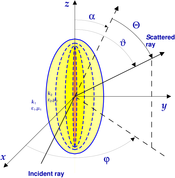
Figure 1: Scattering geometry for a prolate spheroid with the confocal layered structure and $a_{1}/b_{1}=2$. The space is divided into $N+1$ parts: the outer medium (1), the outermost layer (2), $\cdots$, the core ($N+1$). The scattered field in the far-field zone is represented in the spherical coordinate system $(r,\vartheta,\varphi)$. $\Theta$ is the scattering angle. The origin of the Cartesian coordinate system is at the center of the spheroid while the z axis coincides with its axis of revolution. The angle of incidence $\alpha$ is the angle between the direction of incidence and the z axis in the x – z plane.

We consider a plane electromagnetic wave with an arbitrary polarization propagating at an incident angle $\alpha$ to the rotational axis of the spheroid (or the $z$-axis; see Fig. 1). This wave can be represented as a superposition of two components (the magnetic fields can be obtained from the electrical ones by using Maxwell’s equations):
(a) TE mode

$$\vec{E}^{(0)}=-\vec{i}_{y}\exp\left[{ik_{1}(x\sin{\alpha}+z\cos{\alpha})}\right];$$ (4)

(b) TM mode

$$\vec{E}^{(0)}=(\vec{i}_{x}\cos{\alpha}-\vec{i}_{z}\sin{\alpha})\exp\left[{ik_{1}(x\sin{\alpha}+z\cos{\alpha})}\right].$$ (5)

Here $\vec{i}_{x},\,\vec{i}_{y},\,\vec{i}_{z}$ are the unit vectors in the Cartesian coordinate system, $k_{i}=\sqrt{\varepsilon_{i}\mu_{i}}k_{0}$ is the wave number in a medium with the complex permettivity $\varepsilon_{i}$ and the magnetic permeability $\mu_{i}$, $k_{0}=2\pi/\lambda_{0}$ and $k_{1}=2\pi/\lambda_{1}$ are the wave numbers in vacuum and the medium outside the particle, respectively.

As it has been previously shown in [16] (see also [17, 13]), in the case of axisymmetric particles, the scattering problem can be solved independently for each term of the Fourier expansion of the vectors $\vec{E}^{(i)}$ and $\vec{H}^{(i)}$ in terms of the azimuthal angle $\varphi$. In the following, we represent all electromagnetic fields as

$$\vec{E}^{(i)}=\vec{E}^{(i)}_{1}+\vec{E}^{(i)}_{2},\,\,\,\,\,\,\vec{H}^{(i)}=\vec{H}^{(i)}_{1}+\vec{H}^{(i)}_{2},\,\,\,\,\,\,i=0,1,2,\ldots,N+1$$ (6)

so that $\vec{E}^{(i)}_{1}$ and $\vec{H}^{(i)}_{1}$ are independent of the azimuthal angle $\varphi$ (the zeroth term of the Fourier series), whereas the averaging of $\vec{E}^{(i)}_{2}$ and $\vec{H}^{(i)}_{2}$ over $\varphi$ gives zero. Below, the axisymmetric problem for the fields $\vec{E}^{(i)}_{1}$, $\vec{H}^{(i)}_{1}$ and the non-axisymmetric problem for the fields $\vec{E}^{(i)}_{2}$, $\vec{H}^{(i)}_{2}$ are solved independently of one another.

3 Solution to the Axisymmetric Problem

Let us consider the scalar potentials

$${\cal P}^{(i)}=E_{1\varphi}^{(i)}\,\cos\varphi,\,\,\,\,\,\,{\cal Q}^{(i)}=H_{1\varphi}^{(i)}\,\cos\varphi,$$ (7)

where $E_{1\varphi}^{(i)}$, $H_{1\varphi}^{(i)}$ are the $\varphi$-components of the vectors $\vec{E}^{(i)}_{1}$, $\vec{H}^{(i)}_{1}$ ($i=0,1,2,\ldots,N+1$). If we remove the $\cos\varphi$ factor, these potentials coincide with the Abraham potentials within the factor $h_{\varphi}=({d}/{2})\sqrt{(\xi^{2}-\tilde{f})(1-\eta^{2}})$ [16]. It follows from Maxwell’s equations that the scalar potentials satisfy the wave (Helmholtz) equations

$$\Delta{\cal P}^{(i)}+k^{2}_{i}\,{\cal P}^{(i)}=0,\ \ \ \ \Delta{\cal Q}^{(i)}+k^{2}_{i}\,{\cal Q}^{(i)}=0.$$ (8)

The remaining components of the electromagnetic fields $E_{1\varphi}^{(i)}$, $H_{1\varphi}^{(i)}$ can be expressed in terms of their azimuthal components. Note that the axisymmetric problem is solved independently for potentials ${\cal P}$ and ${\cal Q}$, i.e., for the TE and TM waves.

In the case of the TE mode (see Eq. (4)), the boundary conditions (the continuity of the tangential components of the electromagnetic fields at the interfaces) should be rewritten as

$$\left.\begin{array}[]{l}{\cal P}^{(0)}+{\cal P}^{(1)}={\cal P}^{(2)},\\ \displaystyle\frac{\partial\left[\sqrt{\xi^{2}-\tilde{f}}({\cal P}^{(0)}+{\cal P}^{(1)})\right]}{\partial\xi}=\frac{\mu_{1}}{\mu_{2}}\,\frac{\partial\left[\sqrt{\xi^{2}-\tilde{f}}{\cal P}^{(2)}\right]}{\partial\xi},\end{array}\right\}_{\xi=\xi_{1}}$$ (9)

$$\left.\begin{array}[]{l}{\cal P}^{(j)}={\cal P}^{(j+1)},\\ \displaystyle\frac{\partial\left[\sqrt{\xi^{2}-\tilde{f}}{\cal P}^{(j)}\right]}{\partial\xi}=\frac{\mu_{j}}{\mu_{j+1}}\,\frac{\partial\left[\sqrt{\xi^{2}-\tilde{f}}{\cal P}^{(j+1)}\right]}{\partial\xi},\\ \end{array}\right\}_{\xi=\xi_{j}}$$ (10)

where $j=2,3,\ldots,N$.

Let us next formulate the problem in the form of surface integral equations. We can represent the potential ${\cal P}^{(j)}$ of the radiation in the ($j-1$)th shell of the particle as ($j=2,3,\ldots,N+1$)

$${\cal P}^{(j)}={\cal P}^{(j)}_{\rm A}+{\cal P}^{(j)}_{\rm B},$$ (11)

where ${\cal P}^{(j)}_{\rm A}$ has no singularities in the region $D_{j-1}$ (and hence in the region $D_{j}$ enclosed by the surface $S_{j}$) and the potential ${\cal P}^{(j)}_{\rm B}$ satisfies the radiation condition at infinity. Note that inside the core ${\cal P}^{(N+1)}={\cal P}^{(N+1)}_{\rm A}$, that is, ${\cal P}^{(N+1)}_{\rm B}=0$. Within the framework of EBCM, we obtain the system of surface integral equations (see [6] for more details)

$$\frac{d}{2}\,(\xi^{2}_{1}-\tilde{f})\int_{0}^{2\pi}\int_{0}^{\pi}\left\{{\cal P}^{(2)}\left(\vec{r}^{\,\prime}\right)\frac{\partial G_{1}}{\partial\xi^{\prime}}-\left[\frac{\mu_{1}}{\mu_{2}}\,\frac{\partial{\cal P}^{(2)}\left(\vec{r}^{\,\prime}\right)}{\partial\xi^{\prime}}+\left(\frac{\mu_{1}}{\mu_{2}}-1\right)\right.\right.$$

$$\left.\left.\times\frac{\xi_{1}}{(\xi^{2}_{1}-\tilde{f})}\,{\cal P}^{(2)}\left(\vec{r}^{\,\prime}\right)\right]G_{1}\right\}{\rm d}\eta^{\prime}{\rm d}\varphi^{\prime}=\left\{\begin{array}[]{lcl}-{\cal P}^{(0)}(\vec{r}),\ \ \ \vec{r}\in{D_{1}},\\ \phantom{-}{\cal P}^{(1)}(\vec{r}),\ \ \ \vec{r}\in R^{3}\setminus\bar{D_{1}},\end{array}\right.$$ (14)

where $\xi^{\prime}=\xi_{1}$,

$$\frac{d}{2}\,(\xi^{2}_{j}-\tilde{f})\int_{0}^{2\pi}\int_{0}^{\pi}\left\{{\cal P}^{(j+1)}\left(\vec{r}^{\,\prime}\right)\frac{\partial G_{j}}{\partial\xi^{\prime}}-\left[\frac{\mu_{j}}{\mu_{j+1}}\,\frac{\partial{\cal P}^{(j+1)}\left(\vec{r}^{\,\prime}\right)}{\partial\xi^{\prime}}+\left(\frac{\mu_{j}}{\mu_{j+1}}-1\right)\right.\right.$$

$$\left.\left.\times\frac{\xi_{j}}{(\xi^{2}_{j}-\tilde{f})}\,{\cal P}^{(j+1)}\left(\vec{r}^{\,\prime}\right)\right]G_{j}\right\}{\rm d}\eta^{\prime}{\rm d}\varphi^{\prime}=\left\{\begin{array}[]{lcl}-{\cal P}^{(j)}_{\rm A}(\vec{r}),\ \ \ \vec{r}\in{D_{j}},\\ \phantom{-}{\cal P}^{(j)}_{\rm B}(\vec{r}),\ \ \ \vec{r}\in R^{3}\setminus\bar{D_{j}},\end{array}\right.$$ (17)

where $\xi^{\prime}=\xi_{j}$,

$$G_{j}=G(k_{j},\vec{r},\vec{r}^{\,\prime})=\frac{\exp{ik_{j}|\vec{r}-\vec{r}^{\,\prime}|}}{4\pi|\vec{r}-\vec{r}^{\,\prime}|}$$ (18)

is the Green function of the wave equation with the wave number $k_{j}$, $j=2,3,\ldots,N$.

The scalar potentials can be expanded in terms of the spheroidal functions [15]

$$\begin{array}[]{l}{\cal P}^{(0)}\\ {\cal Q}^{(0)}\end{array}=\sum_{l=1}^{\infty}\ \begin{array}[]{l}a^{(0)}_{l}\\ b^{(0)}_{l}\end{array}R_{1l}^{(1)}(c_{1},\xi)\ S_{1l}(c_{1},\eta)\ \cos\varphi,$$ (19)

$$\begin{array}[]{l}{\cal P}^{(1)}\\ {\cal Q}^{(1)}\end{array}=\sum_{l=1}^{\infty}\ \begin{array}[]{l}a^{(1)}_{l}\\ b^{(1)}_{l}\end{array}R_{1l}^{(3)}(c_{1},\xi)\ S_{1l}(c_{1},\eta)\ \cos\varphi,$$ (20)

$$\begin{array}[]{l}{\cal P}^{(j)}_{\rm A}\\ {\cal Q}^{(j)}_{\rm A}\end{array}=\sum_{l=1}^{\infty}\ \begin{array}[]{l}a^{(j)}_{l}\\ b^{(j)}_{l}\end{array}R_{1l}^{(1)}(c_{j},\xi)\ S_{1l}(c_{j},\eta)\ \cos\varphi,$$ (21)

$$\begin{array}[]{l}{\cal P}^{(j)}_{\rm B}\\ {\cal Q}^{(j)}_{\rm B}\end{array}=\sum_{l=1}^{\infty}\ \begin{array}[]{l}c^{(j)}_{l}\\ d^{(j)}_{l}\end{array}R_{1l}^{(3)}(c_{j},\xi)\ S_{1l}(c_{j},\eta)\ \cos\varphi,$$ (22)

where $j=2,3,\ldots,N+1$. For the incident radiation we obtain the following coefficients [17, 13]:
(a) TE mode (see Eq. (4))

$$\begin{array}[]{l}a^{(0)}_{l}=-2i^{l}N_{1l}^{-2}(c_{1})S_{1l}(c_{1},\cos{\alpha}),\,\,\,b^{(0)}_{l}=0;\end{array}$$ (23)

(b) TM mode (see Eq. (5))

$$\begin{array}[]{l}a^{(0)}_{l}=0,\,\,\,\,\displaystyle b^{(0)}_{l}=2i^{l}\sqrt{\frac{\varepsilon_{1}}{\mu_{1}}}N^{-2}_{1l}(c_{1})S_{1l}(c_{1},\cos{\alpha}).\end{array}$$ (24)

Here, $R_{ml}^{(1),(3)}(c_{j},\xi)$ are the prolate radial spheroidal functions of the first and third kinds, $S_{ml}(c_{j},\eta)$ the prolate angular functions with the normalization coefficients $N_{ml}(c_{j})$ [15], and the parameter $c_{j}=k_{j}(d/2)$.

For the expansion of the Green function in terms of the spheroidal functions, we have [15]:

$$G(k_{j},\vec{r},\vec{r}^{\,\prime}) = \frac{ik_{j}}{2\pi}\sum_{m=0}^{\infty}\sum_{l=m}^{\infty}(2-\delta_{0m})\,N_{ml}^{-2}(c_{j})\,R_{ml}^{(1)}(c_{j},\xi_{<})\,R_{ml}^{(3)}(c_{j},\xi_{>})\,$$ (25)

$$\times S_{ml}(c_{j},\eta)\,S_{ml}(c_{j},\eta^{\prime})\,\cos m(\varphi-\varphi^{\prime}),$$

where

$$\delta_{0m}=\left\{\begin{array}[]{l}1,\ \ m=0,\\ 0,\ \ m\neq 0,\end{array}\right.$$

and $\xi_{<}=\min(\xi,\xi^{\prime}),\,\xi_{>}=\max(\xi,\xi^{\prime}).$

We substitute Eqs. (19)–(22), and (25) into the integral equations (14), (17). Taking into account orthogonality of the angular spheroidal functions $S_{ml}(c_{j},\eta)\cos m\varphi$ on the surface of any spheroid, we obtain the linear algebraic equations for the unknown expansion coefficients of the potentials considered. In the matrix notation, they have the following form ($j=1,2,\ldots,N$):

$$\left(\begin{array}[]{c}\vec{z}^{(j)}_{\rm A}\\ \vec{z}^{(j)}_{\rm B}\end{array}\right)={-{\cal A}^{(j)}_{31}-{\cal A}^{(j)}_{33}\choose{\cal A}^{(j)}_{11}\ \ \ \ \ \ {\cal A}^{(j)}_{13}}\ \left(\begin{array}[]{c}\vec{z}^{(j+1)}_{\rm A}\\ \vec{z}^{(j+1)}_{\rm B}\end{array}\right),$$ (26)

where

$${\cal A}^{(j)}_{31} = {\cal W}_{j}\ \left[{\cal R}^{[3]}(c_{j},\xi_{j})\ \Delta^{(1)}(c_{j},c_{j+1})-\frac{\mu_{j}}{\mu_{j+1}}\Delta^{(1)}(c_{j},c_{j+1})\ {\cal R}^{[1]}(c_{j+1},\xi_{j})\right.$$ (27)

$$\left.-\left(\frac{\mu_{j}}{\mu_{j+1}}-1\right)\ \frac{\xi_{j}}{\xi^{2}_{j}-\tilde{f}}\ \Delta^{(1)}(c_{j},c_{j+1})\right]\ {\cal P}^{[1]}(c_{j+1},\xi_{j},\xi_{j+1}),$$

$${\cal A}^{(j)}_{33} = {\cal W}_{j}\ \left[{\cal R}^{[3]}(c_{j},\xi_{j})\ \Delta^{(1)}(c_{j},c_{j+1})-\frac{\mu_{j}}{\mu_{j+1}}\Delta^{(1)}(c_{j},c_{j+1})\ {\cal R}^{[3]}(c_{j+1},\xi_{j})\right.$$ (28)

$$\left.-\left(\frac{\mu_{j}}{\mu_{j+1}}-1\right)\ \frac{\xi_{j}}{\xi^{2}_{j}-\tilde{f}}\ \Delta^{(1)}(c_{j},c_{j+1})\right]\ {\cal P}^{[3]}(c_{j+1},\xi_{j},\xi_{j+1}),$$

$${\cal A}^{(j)}_{11} = {\cal W}_{j}\ \left[{\cal R}^{[1]}(c_{j},\xi_{j})\ \Delta^{(1)}(c_{j},c_{j+1})-\frac{\mu_{j}}{\mu_{j+1}}\Delta^{(1)}(c_{j},c_{j+1})\ {\cal R}^{[1]}(c_{j+1},\xi_{j})\right.$$ (29)

$$\left.-\left(\frac{\mu_{j}}{\mu_{j+1}}-1\right)\ \frac{\xi_{j}}{\xi^{2}_{j}-\tilde{f}}\ \Delta^{(1)}(c_{j},c_{j+1})\right]\ {\cal P}^{[1]}(c_{j+1},\xi_{j},\xi_{j+1}),$$

$${\cal A}^{(j)}_{13} = {\cal W}_{j}\ \left[{\cal R}^{[1]}(c_{j},\xi_{j})\ \Delta^{(1)}(c_{j},c_{j+1})-\frac{\mu_{j}}{\mu_{j+1}}\Delta^{(1)}(c_{j},c_{j+1})\ {\cal R}^{[3]}(c_{j+1},\xi_{j})\right.$$ (30)

$$\left.-\left(\frac{\mu_{j}}{\mu_{j+1}}-1\right)\ \frac{\xi_{j}}{\xi^{2}_{j}-\tilde{f}}\ \Delta^{(1)}(c_{j},c_{j+1})\right]\ {\cal P}^{[3]}(c_{j+1},\xi_{j},\xi_{j+1}).$$

Above, we introduce the vectors specified by

$$\left(\begin{array}[]{c}\vec{z}^{(1)}_{\rm A}\\ \vec{z}^{(1)}_{\rm B}\end{array}\right)=\left(\begin{array}[]{c}\left\{a^{(0)}_{l}R^{(1)}_{1l}(c_{1},\xi_{1})\,N_{1l}(c_{1})\right\}^{\infty}_{1\phantom{{}_{k}}}\\ \left\{a^{(1)}_{l}R^{(3)}_{1l}(c_{1},\xi_{1})\,N_{1l}(c_{1})\right\}^{\infty}_{1}\end{array}\right),$$ (31)

$$\left(\begin{array}[]{c}\vec{z}^{(j)}_{\rm A}\\ \vec{z}^{(j)}_{\rm B}\end{array}\right)=\left(\begin{array}[]{c}\left\{a^{(j)}_{l}R^{(1)}_{1l}(c_{j},\xi_{j})\,N_{1l}(c_{j})\right\}^{\infty}_{1\phantom{{}_{k}}}\\ \left\{c^{(j)}_{l}R^{(3)}_{1l}(c_{j},\xi_{j})\,N_{1l}(c_{j})\right\}^{\infty}_{1}\end{array}\right),$$ (32)

where $j=2,\ldots,N$ and the diagonal matrices

$${\cal R}^{[i]}(c_{j},\xi_{j})=\left\{{R^{(i)}_{ml}}^{\prime}(c_{j},\xi_{j})/R^{(i)}_{ml}(c_{j},\xi_{j})\delta_{nl}\right\}^{\infty}_{m},$$ (33)

$${\cal W}_{j}=-\left[{\cal R}^{[3]}(c_{j},\xi_{j})-{\cal R}^{[1]}(c_{j},\xi_{j})\right]^{-1},$$ (34)

$${\cal P}^{[i]}(c_{j},\xi_{j-1},\xi_{j})=\left\{R^{(i)}_{ml}(c_{j},\xi_{j-1})/R^{(i)}_{ml}(c_{j},\xi_{j})\delta_{nl}\right\}^{\infty}_{m}.$$ (35)

The matrix elements $\Delta^{(m)}(c_{j},c_{j+1})=\left\{\delta^{(m)}_{nl}(c_{j},c_{j+1})\right\}^{\infty}_{m\phantom{{}_{k}}}$ are integrals of the products of the angular spheroidal functions [13]. To derive Eq. (34), we use expression for the Wronskian of the radial spheroidal functions [15]. Since $\vec{z}^{(N+1)}_{\rm B}=0$, the system of equations (26) can be easily solved relative to the expansion coefficients of the scattered radiation potential

$$\vec{z}^{(1)}_{\rm B}={\cal A}_{2}{\cal A}_{1}^{(-1)}\ \vec{z}^{(1)}_{\rm A},$$ (36)

where the coefficients of the incident radiation are given by Eq. (23). The matrices ${\cal A}_{1}$ and ${\cal A}_{2}$ satisfy the relation

$${{\cal A}_{1}\choose{\cal A}_{2}}={-{\cal A}^{(1)}_{31}-{\cal A}^{(1)}_{33}\choose{\cal A}^{(1)}_{11}\ \ \ \ \ \ {\cal A}^{(1)}_{13}}\ \cdots\ {-{\cal A}^{(j)}_{31}-{\cal A}^{(j)}_{33}\choose{\cal A}^{(j)}_{11}\ \ \ \ \ \ {\cal A}^{(j)}_{13}}\ \cdots\ {-{\cal A}^{(N-1)}_{31}-{\cal A}^{(N-1)}_{33}\choose{\cal A}^{(N-1)}_{11}\ \ \ \ \ \ {\cal A}^{(N-1)}_{13}}{-{\cal A}^{(N)}_{31}\choose\ \ {\cal A}^{(N)}_{11}}.$$ (37)

An important point is that the representation of Eqs. (36), (37) in the recursive form needs only one matrix inversion in contrast with the T-matrix representation that requires inversions for each layer and one more at the last step (see discussion in [1]).

For TM mode, the transformation of the above equations for potentials ${\cal Q}^{(j)}$ is performed by the replacements $\mu_{j}\rightarrow\varepsilon_{j},\,\,\,\varepsilon_{j}\rightarrow\mu_{j}$, $a^{(j)}_{l}\rightarrow b^{(j)}_{l}$, and $c^{(j)}_{l}\rightarrow d^{(j)}_{l}$. In order to obtain the corresponding systems for oblate spheroid one must use the standard replacements $c\rightarrow-ic$, $\xi\rightarrow i\xi$ and oblate spheroidal functions instead of the prolate ones. For example, in the case of oblate spheroids and TM mode, Eq. (27) can be written as:

$${\cal A}^{(j)}_{31} = {\cal W}_{j}\ \left[{\cal R}^{[3]}(-ic_{j},i\xi_{j})\ \Delta^{(1)}(-ic_{j},-ic_{j+1})-\frac{\varepsilon_{j}}{\varepsilon_{j+1}}\Delta^{(1)}(-ic_{j},-ic_{j+1})\ {\cal R}^{[1]}(-ic_{j+1},i\xi_{j})\right.$$

$$\left.-\left(\frac{\varepsilon_{j}}{\varepsilon_{j+1}}-1\right)\ \frac{i\xi_{j}}{(i\xi)^{2}_{j}-\tilde{f}}\ \Delta^{(1)}(-ic_{j},-ic_{j+1})\right]\ {\cal P}^{[1]}(-ic_{j+1},i\xi_{j},i\xi_{j+1}).$$

4 Solution to the Non-Axisymmetric Problem

The second terms in Eqs. (6) can be represented in the following form:
(a) TE mode

$$\vec{E}^{(i)}_{2} = \vec{\nabla}\times\left({U}^{(i)}\vec{i}_{z}+{V}^{(i)}\vec{r}\right),$$

$$\vec{H}^{(i)}_{2} = \frac{1}{i\mu_{i}k_{0}}\vec{\nabla}\times\vec{\nabla}\times\left({U}^{(i)}\vec{i}_{z}+{V}^{(i)}\vec{r}\right);$$ (38)

(b) TM mode

$$\vec{E}^{(i)}_{2} = -\frac{1}{i\varepsilon_{i}k_{0}}\vec{\nabla}\times\vec{\nabla}\times\left({U}^{(i)}\vec{i}_{z}+{V}^{(i)}\vec{r}\right),$$

$$\vec{H}^{(i)}_{2} = \vec{\nabla}\times\left({U}^{(i)}\vec{i}_{z}+{V}^{(i)}\vec{r}\right),$$ (39)

where the scalar potentials ${U}^{(i)}$ and ${V}^{(i)}$ satisfy the Helmholtz equations (8).

In the case of TE mode (see Eq. (4)), the boundary conditions for scalar potentials have the form

$$\begin{array}[t]{rl}\left.\begin{array}[]{r}\displaystyle\eta U^{(j)}+\frac{d}{2}\xi V^{(j)}=\eta U^{(j+1)}+\frac{d}{2}\xi V^{(j+1)},\\ \displaystyle\frac{\partial{}}{\partial{\xi}}\left(\xi U^{(j)}+\tilde{f}\frac{d}{2}\eta V^{(j)}\right)=\frac{\partial{}}{\partial{\xi}}\left(\xi U^{(j+1)}+\tilde{f}\frac{d}{2}\eta V^{(j+1)}\right),\\ \displaystyle\varepsilon_{j}\left(\xi U^{(j)}+\tilde{f}\frac{d}{2}\eta V^{(j)}\right)=\varepsilon_{j+1}\left(\xi U^{(j+1)}+\tilde{f}\frac{d}{2}\eta V^{(j+1)}\right),\\ \displaystyle\frac{1}{\mu_{j}}\frac{\partial{}}{\partial{\xi}}\left(\eta U^{(j)}+\frac{d}{2}\xi V^{(j)}\right)=\frac{1}{\mu_{j+1}}\left[\frac{\partial{}}{\partial{\xi}}\left(\eta U^{(j+1)}+\frac{d}{2}\xi V^{(j+1)}\right)\right.\\ \displaystyle+\left.\left(1-\frac{c_{j+1}^{2}}{c^{2}_{j}}\right)\frac{1-\eta^{2}}{\xi^{2}-\tilde{f}}\frac{\partial{}}{\partial{\eta}}\left(\xi U^{(j+1)}+\tilde{f}\frac{d}{2}\eta V^{(j+1)}\right)\right],\end{array}\right\}_{\xi=\xi_{j}}\end{array}$$ (40)

where $j=2,3,\ldots,N$. The boundary conditions for the potentials $U^{(0)},U^{(1)}$ and $V^{(0)},V^{(1)}$ can be written in a similar way to the axisymmetric part (see Eqs. (9), (10)).

As in the case of the axisymmetric part, we can derive the integral equations for the scalar potentials $U^{(j)}$ and $V^{(j)}$

$$\frac{d}{2}\,(\xi^{2}_{j}-\tilde{f})\int_{0}^{2\pi}\int_{0}^{\pi}\left\{U^{(j+1)}\frac{\partial G_{j}}{\partial\xi^{\prime}}-\frac{\mu_{j}}{\mu_{j+1}}\frac{\partial U^{(j+1)}}{\partial\xi^{\prime}}G_{j}+\left(\frac{\varepsilon_{j+1}}{\varepsilon_{j}}-1\right)\left[\frac{\xi_{j}^{2}}{\xi_{j}^{2}-\tilde{f}\eta^{\prime^{2}}}\,U^{(j+1)}\right.\right.$$

$$\left.\left.+\frac{\tilde{f}\xi_{j}\eta^{\prime}}{\xi_{j}^{2}-\tilde{f}\eta^{\prime^{2}}}\,\frac{d}{2}\,V^{(j+1)}\right]\frac{\partial G_{j}}{\partial\xi^{\prime}}+\left(\frac{\mu_{j}}{\mu_{j+1}}-1\right)\left[\frac{\xi_{j}^{2}}{\xi_{j}^{2}-\tilde{f}\eta^{\prime^{2}}}\frac{\partial{U^{(j+1)}}}{\partial{\xi^{\prime}}}+\frac{\tilde{f}\xi_{j}\eta^{\prime}}{\xi_{j}^{2}-\tilde{f}\eta^{\prime^{2}}}\,\frac{d}{2}\,\frac{\partial{V^{(j+1)}}}{\partial{\xi^{\prime}}}\right]G_{j}\right.$$

$$\left.+\left(\frac{\varepsilon_{j+1}}{\varepsilon_{j}}-1\right)\frac{\xi_{j}}{\xi_{j}^{2}-\tilde{f}\eta^{\prime^{2}}}\left[-U^{(j+1)}+\frac{2\xi_{j}^{2}}{\xi_{j}^{2}-\tilde{f}\eta^{\prime^{2}}}\,U^{(j+1)}+\frac{2\tilde{f}\xi_{j}\eta^{\prime}}{\xi_{j}^{2}-\tilde{f}\eta^{\prime^{2}}}\,\frac{d}{2}\,V^{(j+1)}\right]G_{j}\right.$$

$$\left.-\left(\frac{\varepsilon_{j+1}}{\varepsilon_{j}}-\frac{\mu_{j}}{\mu_{j+1}}\right)\frac{\tilde{f}\eta^{\prime}}{\xi_{j}^{2}-\tilde{f}\eta^{\prime^{2}}}\left[\frac{1-\eta^{\prime^{2}}}{\xi_{j}^{2}-\tilde{f}}\frac{\partial{}}{\partial{\eta^{\prime}}}\left(\xi_{j}\,U^{(j+1)}+\tilde{f}\eta^{\prime}\,\frac{d}{2}\,V^{(j+1)}\right)+\frac{d}{2}\,V^{(j+1)}\right]G_{j}\right\}{\rm d}\eta^{\prime}{\rm d}\varphi^{\prime}$$

$$=\left\{\begin{array}[]{lcl}-U^{(j)}_{\rm A}(\vec{r}),\ \ \ \ \ \ \vec{r}\in{D_{j}},\\ U^{(j)}_{\rm B}(\vec{r}),\ \ \ \vec{r}\in R^{3}\setminus\bar{D_{j}},\end{array}\right.$$ (43)

$$\frac{d}{2}\,(\xi^{2}_{j}-\tilde{f})\int_{0}^{2\pi}\int_{0}^{\pi}\left\{\frac{\varepsilon_{j+1}}{\varepsilon_{j}}\,\frac{d}{2}\,V^{(j+1)}\frac{\partial G_{j}}{\partial\xi^{\prime}}-\frac{d}{2}\,\frac{\partial V^{(j+1)}}{\partial\xi^{\prime}}G_{j}-\left(\frac{\varepsilon_{j+1}}{\varepsilon_{j}}-1\right)\left[\frac{\xi_{j}\eta^{\prime}}{\xi_{j}^{2}-\tilde{f}\eta^{\prime^{2}}}\,U^{(j+1)}\right.\right.$$

$$\left.\left.+\frac{\xi_{j}^{2}}{\xi_{j}^{2}-\tilde{f}\eta^{\prime^{2}}}\,\frac{d}{2}\,V^{(j+1)}\right]\frac{\partial G_{j}}{\partial\xi^{\prime}}-\left(\frac{\mu_{j}}{\mu_{j+1}}-1\right)\left[\frac{\xi_{j}\eta^{\prime}}{\xi_{j}^{2}-\tilde{f}\eta^{\prime^{2}}}\frac{\partial{U^{(j+1)}}}{\partial{\xi^{\prime}}}+\frac{\xi_{j}^{2}}{\xi_{j}^{2}-\tilde{f}\eta^{\prime^{2}}}\,\frac{d}{2}\,\frac{\partial{V^{(j+1)}}}{\partial{\xi^{\prime}}}\right]G_{j}\right.$$

$$\left.-\left(\frac{\varepsilon_{j+1}}{\varepsilon_{j}}-1\right)\frac{\xi_{j}}{\xi_{j}^{2}-\tilde{f}\eta^{\prime^{2}}}\left[-\frac{d}{2}\,V^{(j+1)}+\frac{2\xi_{j}\eta^{\prime}}{\xi_{j}^{2}-\tilde{f}\eta^{\prime^{2}}}\,U^{(j+1)}+\frac{2\xi_{j}^{2}}{\xi_{j}^{2}-\tilde{f}\eta^{\prime^{2}}}\,\frac{d}{2}\,V^{(j+1)}\right]G_{j}\right.$$

$$\left.+\left(\frac{\varepsilon_{j+1}}{\varepsilon_{j}}-\frac{\mu_{j}}{\mu_{j+1}}\right)\frac{\xi}{\xi_{j}^{2}-\tilde{f}\eta^{\prime^{2}}}\left[\frac{1-\eta^{\prime^{2}}}{\xi_{j}^{2}-\tilde{f}}\frac{\partial{}}{\partial{\eta^{\prime}}}\left(\xi_{j}\,U^{(j+1)}+\tilde{f}\eta^{\prime}\,\frac{d}{2}\,V^{(j+1)}\right)+\frac{d}{2}\,V^{(j+1)}\right]G_{j}\right\}{\rm d}\eta^{\prime}{\rm d}\varphi^{\prime}$$

$$=\left\{\begin{array}[]{lcl}-V^{(j)}_{\rm A}(\vec{r}),\ \ \ \ \ \ \vec{r}\in{D_{j}},\\ V^{(j)}_{\rm B}(\vec{r}),\ \ \ \vec{r}\in R^{3}\setminus\bar{D_{j}},\end{array}\right.$$ (46)

where $\xi^{\prime}=\xi_{j}$.

The scalar potentials are expanded in terms of the spheroidal functions [15]

$$\begin{array}[]{l}U^{(0)}\\ V^{(0)}\end{array}=\sum_{m=1}^{\infty}\ \sum_{l=m}^{\infty}\ \begin{array}[]{l}a^{(0)}_{ml}\\ b^{(0)}_{ml}\end{array}R_{ml}^{(1)}(c_{1},\xi)\ S_{ml}(c_{1},\eta)\ \cos m\varphi,$$ (47)

$$\begin{array}[]{l}U^{(1)}\\ V^{(1)}\end{array}=\sum_{m=1}^{\infty}\ \sum_{l=m}^{\infty}\ \begin{array}[]{l}a^{(1)}_{ml}\\ b^{(1)}_{ml}\end{array}R_{ml}^{(3)}(c_{1},\xi)\ S_{ml}(c_{1},\eta)\ \cos m\varphi,$$ (48)

$$\begin{array}[]{l}U^{(j)}_{\rm A}\\ V^{(j)}_{\rm A}\end{array}=\sum_{m=1}^{\infty}\ \sum_{l=m}^{\infty}\ \begin{array}[]{l}a^{(j)}_{ml}\\ b^{(j)}_{ml}\end{array}R_{ml}^{(1)}(c_{j},\xi)\ S_{ml}(c_{j},\eta)\ \cos m\varphi,$$ (49)

$$\begin{array}[]{l}U^{(j)}_{\rm B}\\ V^{(j)}_{\rm B}\end{array}=\sum_{m=1}^{\infty}\ \sum_{l=m}^{\infty}\ \begin{array}[]{l}c^{(j)}_{ml}\\ d^{(j)}_{ml}\end{array}R_{ml}^{(3)}(c_{j},\xi)\ S_{ml}(c_{j},\eta)\ \cos m\varphi,$$ (50)

where $j=2,3,\ldots,N+1$. For the TE mode, the coefficients that describe the incident radiation are equal to (see [17, 13])

$${a}^{(0)}_{ml}=\frac{4i^{l-1}}{k_{1}}N^{-2}_{ml}(c_{1})\frac{S_{ml}(c_{1},\cos{\alpha})}{\sin{\alpha}}\,,\,\,\,{b}^{(0)}_{ml}=0.$$ (51)

For TM mode, the coefficients ${a}^{(0)}_{ml}$ have the opposite sign and the multiplicand $\sqrt{{\varepsilon_{1}}/{\mu_{1}}}$ (see Eqs. (5), (39)).

Substituting Eqs. (47)–(50), and (25) into integral equations (43) and (46), we obtain infinite systems relative to the unknown expansion coefficients. The systems can be written in the matrix form ($j=1,2,\ldots,N$)

$$\left(\begin{array}[]{c}\vec{Z}^{(j)}_{\rm A}\\ \vec{Z}^{(j)}_{\rm B}\end{array}\right)={-{\cal A}^{(j)}_{31}-{\cal A}^{(j)}_{33}\choose{\cal A}^{(j)}_{11}\ \ \ \ \ \ {\cal A}^{(j)}_{13}}\left(\begin{array}[]{c}\vec{Z}^{(j+1)}_{\rm A}\\ \vec{Z}^{(j+1)}_{\rm B}\end{array}\right),$$ (52)

where the vectors and matrices have the block structure

$$\left(\begin{array}[]{c}\vec{Z}^{(j)}_{\rm A}\\ \vec{Z}^{(j)}_{\rm B}\end{array}\right)=\left(\begin{array}[]{c}\left\{k_{1}{a}^{(j)}_{ml}R^{(3)}_{ml}(c_{j},\xi_{j})N_{ml}(c_{j})\right\}^{\infty}_{m\phantom{{}_{k}}}\\ \left\{c_{1}{b}^{(j)}_{ml}R^{(3)}_{ml}(c_{j},\xi_{j})N_{ml}(c_{j})\right\}^{\infty}_{m\phantom{{}_{k}}}\\ \left\{k_{1}{c}^{(j)}_{ml}R^{(3)}_{ml}(c_{j},\xi_{j})N_{ml}(c_{j})\right\}^{\infty}_{m\phantom{{}_{k}}}\\ \left\{c_{1}{d}^{(j)}_{ml}R^{(3)}_{ml}(c_{j},\xi_{j})N_{ml}(c_{j})\right\}^{\infty}_{m}\end{array}\right),$$ (53)

$${\cal A}^{(j)}_{ik}={\mathfrak{A}^{(j)}_{ik,{\rm A}}\ \ \ \mathfrak{B}^{(j)}_{ik,{\rm A}}\choose\mathfrak{A}^{(j)}_{ik,{\rm B}}\ \ \ \mathfrak{B}^{(j)}_{ik,{\rm B}}},$$ (54)

$$\mathfrak{A}^{(j)}_{31,{\rm A}} = {\cal W}_{j}\ \left\{{\cal R}^{[3]}(c_{j},\xi_{j})\ \Delta^{(m)}(c_{j},c_{j+1})-\frac{\mu_{j}}{\mu_{j+1}}\Delta^{(m)}(c_{j},c_{j+1})\ {\cal R}^{[1]}(c_{j+1},\xi_{j})\right.$$ (55)

$$+\left(\frac{\varepsilon_{j+1}}{\varepsilon_{j}}-1\right)\xi_{j}\left[\xi_{j}{\cal R}^{[3]}(c_{j},\xi_{j})Q^{(m)}(c_{j},c_{j+1},\xi_{j})\right.$$

$$\left.\left.-Q^{(m)}(c_{j},c_{j+1},\xi_{j})\left(I-2\xi_{j}^{2}Q^{(m)}(c_{j+1},c_{j+1},\xi_{j})\right)\right]\right.$$

$$\left.+\left(\frac{\mu_{j}}{\mu_{j+1}}-1\right)\ \xi_{j}^{2}Q^{(m)}(c_{j},c_{j+1},\xi_{j}){\cal R}^{[1]}(c_{j+1},\xi_{j})\right.$$

$$\left.-\left(\frac{\varepsilon_{j+1}}{\varepsilon_{j}}-\frac{\mu_{j}}{\mu_{j+1}}\right)\ \frac{\tilde{f}\xi_{j}}{\xi^{2}_{j}-\tilde{f}}\ Q^{(m)}(c_{j},c_{j+1},\xi_{j})E^{(m)}(c_{j+1},c_{j+1})\right\}$$

$$\times{\cal P}^{[1]}(c_{j+1},\xi_{j},\xi_{j+1}),$$

$$\mathfrak{B}^{(j)}_{31,{\rm A}} = {\cal W}_{j}\ \left\{\left(\frac{\varepsilon_{j+1}}{\varepsilon_{j}}-1\right)\tilde{f}\xi_{j}\left[{\cal R}^{[3]}(c_{j},\xi_{j})Q^{(m)}(c_{j},c_{j+1},\xi_{j})\right.\right.$$ (56)

$$\left.\left.+2\xi_{j}Q^{(m)}(c_{j},c_{j+1},\xi_{j})Q^{(m)}(c_{j+1},c_{j+1},\xi_{j})\right]\Gamma^{(m)}(c_{j+1},c_{j+1})\right.$$

$$\left.+\left(\frac{\mu_{j}}{\mu_{j+1}}-1\right)\ \tilde{f}\xi_{j}Q^{(m)}(c_{j},c_{j+1},\xi_{j})\Gamma^{(m)}(c_{j+1},c_{j+1}){\cal R}^{[1]}(c_{j+1},\xi_{j})-\left(\frac{\varepsilon_{j+1}}{\varepsilon_{j}}-\frac{\mu_{j}}{\mu_{j+1}}\right)\right.$$

$$\left.\times\frac{\tilde{f}}{\xi^{2}_{j}-\tilde{f}}\ \left[(\xi^{2}_{j}Q^{(m)}(c_{j},c_{j+1},\xi_{j})-\Delta^{(m)}(c_{j},c_{j+1}))K^{(m)}(c_{j+1},c_{j+1})+\Gamma^{(m)}(c_{j},c_{j+1})\right]\right\}\$$

$$\times{\cal P}^{[1]}(c_{j+1},\xi_{j},\xi_{j+1}),$$

$$\mathfrak{A}^{(j)}_{31,{\rm B}} = {\cal W}_{j}\ \left\{-\left(\frac{\varepsilon_{j+1}}{\varepsilon_{j}}-1\right)\xi_{j}\left[{\cal R}^{[3]}(c_{j},\xi_{j})Q^{(m)}(c_{j},c_{j+1},\xi_{j})\right.\right.$$ (57)

$$\left.\left.+2\xi_{j}Q^{(m)}(c_{j},c_{j+1},\xi_{j})Q^{(m)}(c_{j+1},c_{j+1},\xi_{j})\right]\Gamma^{(m)}(c_{j+1},c_{j+1})\right.$$

$$\left.-\left(\frac{\mu_{j}}{\mu_{j+1}}-1\right)\ \xi_{j}Q^{(m)}(c_{j},c_{j+1},\xi_{j})\Gamma^{(m)}(c_{j+1},c_{j+1}){\cal R}^{[1]}(c_{j+1},\xi_{j})+\left(\frac{\varepsilon_{j+1}}{\varepsilon_{j}}-\frac{\mu_{j}}{\mu_{j+1}}\right)\ \right.$$

$$\left.\times\frac{\xi^{2}_{j}}{\xi^{2}_{j}-\tilde{f}}\ Q^{(m)}(c_{j},c_{j+1},\xi_{j})K^{(m)}(c_{j+1},c_{j+1})\right\}\ {\cal P}^{[1]}(c_{j+1},\xi_{j},\xi_{j+1}),$$

$$\mathfrak{B}^{(j)}_{31,{\rm B}} = {\cal W}_{j}\ \left\{\frac{\varepsilon_{j+1}}{\varepsilon_{j}}{\cal R}^{[3]}(c_{j},\xi_{j})\ \Delta^{(m)}(c_{j},c_{j+1})-\Delta^{(m)}(c_{j},c_{j+1})\ {\cal R}^{[1]}(c_{j+1},\xi_{j})\right.$$ (58)

$$\left.-\left(\frac{\varepsilon_{j+1}}{\varepsilon_{j}}-1\right)\xi_{j}\left[\xi_{j}{\cal R}^{[3]}(c_{j},\xi_{j})Q^{(m)}(c_{j},c_{j+1},\xi_{j})\right.\right.$$

$$\left.\left.-Q^{(m)}(c_{j},c_{j+1},\xi_{j})(I-2\xi_{j}^{2}Q^{(m)}(c_{j+1},c_{j+1},\xi_{j}))\right]\right.$$

$$\left.-\left(\frac{\mu_{j}}{\mu_{j+1}}-1\right)\ \xi_{j}^{2}Q^{(m)}(c_{j},c_{j+1},\xi_{j}){\cal R}^{[1]}(c_{j+1},\xi_{j})\right.$$

$$\left.+\left(\frac{\varepsilon_{j+1}}{\varepsilon_{j}}-\frac{\mu_{j}}{\mu_{j+1}}\right)\ \frac{\xi_{j}}{\xi^{2}_{j}-\tilde{f}}\ \left[\tilde{f}Q^{(m)}(c_{j},c_{j+1},\xi_{j})E^{(m)}(c_{j+1},c_{j+1})+\Delta^{(m)}(c_{j},c_{j+1})\right]\right\}\$$

$$\times{\cal P}^{[1]}(c_{j+1},\xi_{j},\xi_{j+1}),$$

$$Q^{(m)}(c_{j+1},c_{j+1},\xi_{j})={\left\{\xi_{j}^{2}I-\tilde{f}\left[\Gamma^{(m)}(c_{j+1},c_{j+1})\right]^{2}\right\}}^{-1},$$ (59)

$$Q^{(m)}(c_{j},c_{j+1},\xi_{j})=\Delta^{(m)}(c_{j},c_{j+1})\,Q^{(m)}(c_{j+1},c_{j+1},\xi_{j})$$ (60)

and $I=\left\{\delta_{nl}\right\}^{\infty}_{m}$ is the unit matrix. Here, $m$ is the azimuthal index that runs from unity to infinity. The subscripts and superscripts of the matrices have the same meaning as in the previous section. The elements of the remaining matrices in Eq. (54) can be obtained from Eqs. (55)–(58) as explained above (see Eqs. (27)–(30)). The matrix elements $\Gamma^{(m)}(c_{j},c_{j})=\left\{\gamma^{(m)}_{nl}(c_{j},c_{j})\right\}^{\infty}_{m}$, $K^{(m)}(c_{j},c_{j})=\left\{\kappa^{(m)}_{nl}(c_{j},c_{j})\right\}^{\infty}_{m}$ and $E^{(m)}(c_{j},c_{j})=\left\{\varepsilon^{(m)}_{nl}(c_{j},c_{j})\right\}^{\infty}_{m}$ are the integrals of products of the angular spheroidal functions and their derivatives (see [17, 13]).

The system (52) can be easily solved for the expansion coefficients of the scattered radiation potential (cf. Eq. (26))

$$\vec{Z}^{(1)}_{\rm B}={\cal A}_{2}{\cal A}_{1}^{(-1)}\ \vec{Z}^{(1)}_{\rm A},$$ (61)

where

$$\vec{Z}^{(1)}_{\rm B}=\left(\begin{array}[]{c}\left\{k_{1}{a}^{(1)}_{ml}R^{(3)}_{ml}(c_{1},\xi_{1})N_{ml}(c_{1})\right\}^{\infty}_{m\phantom{{}_{k}}}\\ \left\{c_{1}{b}^{(1)}_{ml}R^{(3)}_{ml}(c_{1},\xi_{1})N_{ml}(c_{1})\right\}^{\infty}_{m\phantom{{}_{k}}}\end{array}\right),$$ (62)

$$\vec{Z}^{(1)}_{\rm A}=\left(\begin{array}[]{c}\left\{k_{1}{\it a}^{(0)}_{ml}R^{(1)}_{ml}(c_{1},\xi_{1})\,N_{ml}(c_{1})\right\}^{\infty}_{m}\\ 0\end{array}\right),$$ (63)

and the matrices ${\cal A}_{1}$ and ${\cal A}_{2}$ satisfy Eq.(37) but have the block structure (see Eq. (54)).

For the TM mode, we can obtain infinite systems for the unknown expansion coefficients of the scalar potentials by replacing $\mu_{j}\rightarrow\varepsilon_{j},\,\,\varepsilon_{j}\rightarrow\mu_{j}$ in the above relations. Note that in the case of $\mu_{j}=1$, their form is much simpler than in the corresponding case of the TE mode (see also [17, 13]).

5 Characteristics of Scattered Radiation

Using the expansion coefficients of the scattered field for the TE and TM polarizations, we can calculate elements of the scattering matrix (see the corresponding expressions in [13]) and the integral characteristics of the scattered radiation (e.g., the cross sections of a particle for extinction $C_{\rm ext}$, scattering $C_{\rm sca}$, absorption $C_{\rm abs}$, and radiation pressure $C_{\rm pr}$). These cross sections are products of the corresponding efficiency factors $Q$ and the viewing geometric cross section of a spheroid (the area of the particle shadow)

$$C=GQ,$$

where

$$G(\alpha)=\pi b_{1}\left(a_{1}^{2}\sin^{2}\alpha+b_{1}^{2}\cos^{2}\alpha\right)^{1/2}\,\,\,\,\,\,\,\mbox{for prolate spheroids,}$$ (64)

$$G(\alpha)=\pi a_{1}\left(a_{1}^{2}\cos^{2}\alpha+b_{1}^{2}\sin^{2}\alpha\right)^{1/2}\,\,\,\,\,\,\mbox{for oblate spheroids}$$ (65)

and $a_{1}$ and $b_{1}$ are the major and minor semiaxes of a multilayered spheroid. The efficiency factors for extinction can be found as

$$Q_{\rm ext} \,\,=\frac{4}{c^{2}_{1}{\left[(\xi^{2}_{1}-\tilde{f})(\xi^{2}_{1}-\tilde{f}{\cos}^{2}{\alpha})\right]}^{1/2}}\,{\rm Re}\left[-\sum^{\infty}_{l=1}i^{-l}{\it a}^{(1)}_{l}S_{1l}(c_{1},\cos{\alpha})\right.$$ (66)

$$\!\!\!+ \sum^{\infty}_{m=1}\sum^{\infty}_{l=m}i^{-(l-1)}\Bigl{(}k_{1}{\it a}^{(1)}_{ml}S_{ml}(c_{1},\cos{\alpha})+\left.\left.i{\it b}^{(1)}_{ml}S^{{}^{\prime}}_{ml}(c_{1},\cos{\alpha})\right)\sin{\alpha}\Biggr{]}\right.,$$

where, as above, $\tilde{f}=1$ for prolate spheroids and $\tilde{f}=-1$ for oblate ones. Expressions for other factors are given in [17, 13].

To compare the optical properties of particles of various shape, the cross sections can be normalized by the geometric cross section of the equivolume sphere

$$\frac{C}{\pi r^{2}_{V}}=\frac{[(a_{1}/b_{1})^{2}\sin^{2}\alpha+\cos^{2}\alpha]^{1/2}}{(a_{1}/b_{1})^{2/3}}\,Q\,\,\,\,\,\,\,\,\,\,\,\mbox{for prolate spheroids,}$$ (67)

$$\frac{C}{\pi r^{2}_{V}}=\frac{[(a_{1}/b_{1})^{2}\cos^{2}\alpha+\sin^{2}\alpha]^{1/2}}{(a_{1}/b_{1})^{1/3}}\,Q\,\,\,\,\,\,\,\,\,\,\,\mbox{for oblate spheroids.}$$ (68)

Here, $r_{V}$ is the radius of the sphere with the volume equal to that of a given spheroidal particle. This radius can be defined as

$$r_{V}^{3}=a_{1}\,b^{2}_{1}\,\,\,\,\,\,\,\,\,\,\,\mbox{for prolate spheroids,}$$ (69)

$$r_{V}^{3}=a^{2}_{1}\,b_{1}\,\,\,\,\,\,\,\,\,\,\,\mbox{for oblate spheroids.}$$ (70)

The optical properties of a multilayered confocal spheroid can be found if we put the type of spheroid (prolate or oblate), the number of layers $N$, complex refractive indices of all layers $m_{j}=n_{j}+k_{j}i$, the outer aspect ratio $a_{1}/b_{1}$ ($a_{1}$ and $b_{1}$ are the major and minor semiaxes), the total particle size parameter, and the relative ratios of volumes of the layers $f_{j}=V_{j}/V_{\rm total}$. The size parameter may be specified as

$$x_{V}=2\pi r_{V}/\lambda,$$

where $r_{V}$ is the radius of a sphere whose volume is equal to that of the spheroid, $\lambda$ the wavelength of incident radiation.

The radial coordinates $\xi_{j}$ that define the boundaries of a layered particle, are connected with the corresponding semiaxes as

$$\xi_{j}=\left(\frac{a_{j}}{b_{j}}\right)^{(1+\tilde{f})/2}\left[\left(\frac{a_{j}}{b_{j}}\right)^{2}-1\right]^{-1/2}.$$ (71)

The efficiency factors can also be considered as a function of the size parameter $2\pi a_{1}/\lambda$ given by

$$\frac{2\pi a_{1}}{\lambda}=\left(\frac{a_{1}}{b_{1}}\right)^{(1-\tilde{f})/2}\,c_{1}\xi_{1}=x_{V}\,\left(\frac{a_{1}}{b_{1}}\right)^{(3+\tilde{f})/6}.$$ (72)

The ratio of layer volumes inside the surface $j$ ($j=2,3,\ldots,N$) to the total volume of a multilayered particle is determined by using the parameters $\xi_{1}$ and $\xi_{j}$

$$\sum_{l=j}^{N}\,{f_{l}}=\sum_{l=j}^{N}\,\frac{V_{l}}{V_{\rm total}}=\frac{\xi_{j}\,(\xi^{2}_{j}-\tilde{f})}{\xi_{1}\,(\xi^{2}_{1}-\tilde{f})}.$$ (73)

The aspect ratios of internal layers can be calculated from the volume ratios by using the iterative procedure for prolate spheroids

$$(\xi_{j})^{(n)}=\sqrt[3]{(\xi_{j})^{(n-1)}+\sum_{l=j}^{N}\,{f_{l}}\,[\xi_{1}\,(\xi_{1}^{2}-1)]},$$ (74)

where $n=1,\,2\,\ldots$ and the initial value $(\xi_{j})^{(0)}=\xi_{j-1}$. For oblate spheroids, the parameter $\xi_{j}$ can be found by Newton’s method

$$(\xi_{j})^{(n)}=\frac{2\left[(\xi_{j})^{(n-1)}\right]^{3}+\sum_{l=j}^{N}\,{f_{l}}\,[\xi_{1}\,(\xi_{1}^{2}+1)]}{3\left[(\xi_{j})^{(n-1)}\right]^{2}+1},$$ (75)

where $n=1,\,2\,\ldots$ and the initial value $(\xi_{j})^{(0)}=0$.

6 Numerical Results and Discussion

6.1 Computational Tests

The created computer code is based on our codes developed earlier for homogeneous [17] and coated spheroids [13]. In calculations of the radial spheroidal functions, we use their expansions in terms of the Legendre or Bessel functions, the solution to the corresponding differential equation, or Jáffe expansion for prolate functions according to the recommendations given in [18, 19].

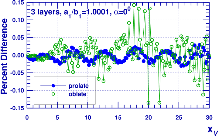
Figure 2: Percent difference between three-layered spheres and three-layered spheroids $\epsilon$ defined by Eq. (76): ${m}_{3}=1.7+0.0i$, ${m}_{2}=1.5+0.0i$, ${m}_{1}=1.3+0.0i$, $V_{j}/V_{\rm total}=0.33$, $a_{1}/b_{1}=1.0001$, $\alpha=0\hbox{${}^{\circ}$}$, ($\bullet$) – prolate spheroids, ($\circ$) – oblate spheroids.

The numerical code has been examined by using various tests that include internal control (see Table 1), a comparison with the known results for homogeneous and core-mantle spheroids and multilayered spheres [20] (Fig. 2) as well as a comparison with the calculations for multilayered spheroids based on the EBCM with a spherical basis [1], the SVM with a spherical basis [3], and the quasistatic approximation [21]. We also have considered absorbing and dielectric particles with a different number of layers and various aspect ratios.

For non-absorbing particles the efficiency factors for extinction and scattering are known to be equal for the same azimuthal index $m$: $Q^{(m)}_{\rm ext}=Q^{(m)}_{\rm sca}$ ($Q=\sum_{m}Q^{(m)}$). Then by increasing the number of terms $N_{\max}$ in sums for $Q^{(m)}_{\rm ext}$ and $Q^{(m)}_{\rm sca}$, one should obtain a decreasing difference between these two factors, i.e., $\left|Q^{(m)}_{\rm ext}-Q^{(m)}_{\rm sca}\right|\rightarrow 0$, if $N_{\max}\rightarrow\infty$. Table 1 shows the behavior of the efficiency factors in the case of radiation propagating along the rotation axis of a spheroid when the sums over $m$ contain only one term, $m=1$. A comparison with the results presented in [13] demonstrates that the convergence for multilayered spheroids resembles that for coated spheroids, i.e, it is not a function of the number of layers $N$. The convergence is determined by the particle size $2\pi a_{1}/\lambda$ and is independent of its shape. The latter feature makes our solution with a spheroidal basis essentially different from the SVM or EBCM approach with spherical basis when convergence quickly degrades for spheroids with aspect ratios $a_{1}/b_{1}\mathrel{\mathchoice{\vbox{\offinterlineskip\halign{\hfil$\displaystyle#$\hfil\cr>\cr\sim\cr}}}{\vbox{\offinterlineskip\halign{\hfil$\textstyle#$\hfil\cr>\cr\sim\cr}}}{\vbox{\offinterlineskip\halign{\hfil$\scriptstyle#$\hfil\cr>\cr\sim\cr}}}{\vbox{\offinterlineskip\halign{\hfil$\scriptscriptstyle#$\hfil\cr>\cr\sim\cr}}}}1.5-2$ [1, 3]. Note that our code allows one to calculate the optical properties of spheroids with the size parameters up to $x_{V}\approx 15-20$ including very elongated or flattened particles. The time of calculations grows with the increase of layers number as $t\approx N^{1.2}$, which is much faster as compared to other methods ($t\approx N^{2.5-3}$ see discussion in [3]).

If the particles are nearly spherical, the optical properties of multilayered spheroids and spheres should be almost the same. We have considered various absorbing and dielectric particles and some results are shown in Fig. 2 where the relative differences in percents

$$\epsilon=\frac{Q_{\rm ext}({\rm sphere})-C_{\rm ext}({\rm spheroid})/\pi r_{V}^{2}}{Q_{\rm ext}({\rm sphere})}\,100\%$$ (76)

are given. The values of $\epsilon$ are plotted as a function of the size parameter $x_{V}$ for particles with the aspect ratio $a_{1}/b_{1}=1.0001$ and the volume ratios $V_{j}/V_{\rm total}=0.33$ ($j=1,2,3$). The aspect ratios of internal layers are equal to $a_{2}/b_{2}\approx 1.00016$ and $a_{3}/b_{3}\approx 1.00021$. The wavelike behavior is typical only for dielectric particles. For highly absorbing particles, the values of $\epsilon$ demonstrate a smooth, monotonous growth with increasing $x_{V}$.

6.2 Particles with a Different Number of Layers

The model of multilayered spheroids gives wide opportunities to investigate both the shape and structure effects on the optics of composite particles simultaneously. As one of the first applications of the developed model, is our analysis of the idea to represent some composite interstellar grains by multilayered particles as suggested in [20]. We consider multilayered spheroids with different material layers cyclically changing inside a particle. The particles are assumed to be composed of amorphous carbon or silicate with varied volume fraction of vacuum. The chosen optical constants for carbon ($m=1.98+0.23i$) and silicate ($m=1.68+0.03i$) correspond to the wavelength $\lambda=0.55\,\mu$m.

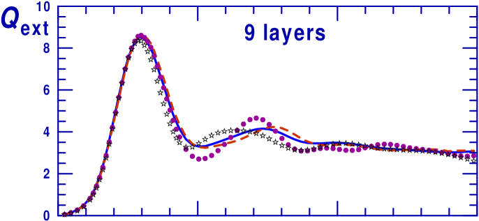
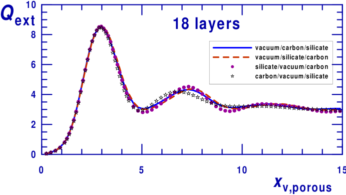
Figure 3: Size dependence of the extinction efficiency factors for layered prolate spheroids with $a_{1}/b_{1}=3$. Each particle contains an equal fraction of carbon, silicate, and vacuum (the porosity ${\cal P}=1/3$) separated in equivolume confocal layers. The cyclic order of the different material layers is indicated (starting from the core). The effect of the increase of the number of layers is illustrated.

The extinction efficiencies of equivolume layered prolate spheroids with $a_{1}/b_{1}=3$ are compared in Fig. 3. In this case, the aspect ratio of the innermost layer is equal to $a_{3}/b_{3}=4.91$, $a_{9}/b_{9}=8.33$ and $a_{18}/b_{18}=11.72$ for 3-layered, 9-layered and 18-layered particles, respectively.

The size parameters of compact and porous particles are related as

$$x_{\rm porous}=\frac{x_{\rm compact}}{(1-{\cal P})^{1/3}}=\frac{x_{\rm compact}}{(V_{\rm solid}/V_{\rm total})^{1/3}},$$ (77)

where the particle porosity ${\cal P}$ ($0\leq{\cal P}<1$) is introduced as ${\cal P}=V_{\rm vac}/V_{\rm total}=1-V_{\rm solid}/V_{\rm total}$ and $V_{\rm vac}$ and $V_{\rm solid}$ are the volume fractions of vacuum and solid material, respectively.

As in the case of layered spheres (see [20, 22]), the scattering characteristics of layered spheroids slightly depend on the order of materials and become close to some “average” ones, when particles consist of many layers ($\mathrel{\mathchoice{\vbox{\offinterlineskip\halign{\hfil$\displaystyle#$\hfil\cr>\cr\sim\cr}}}{\vbox{\offinterlineskip\halign{\hfil$\textstyle#$\hfil\cr>\cr\sim\cr}}}{\vbox{\offinterlineskip\halign{\hfil$\scriptstyle#$\hfil\cr>\cr\sim\cr}}}{\vbox{\offinterlineskip\halign{\hfil$\scriptscriptstyle#$\hfil\cr>\cr\sim\cr}}}}15-20$).

The convergence of the extinction factors seems to be better for oblique incidence and oblate particles and larger aspect ratios. Such a behavior is typical for other efficiencies (scattering, absorption), albedo and the asymmetry parameter.

6.3 Particles of Different Porosity

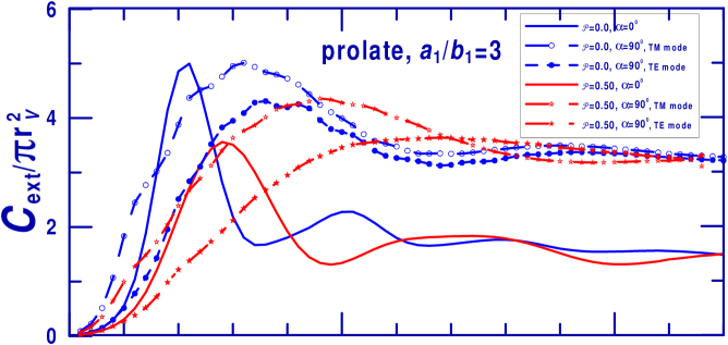
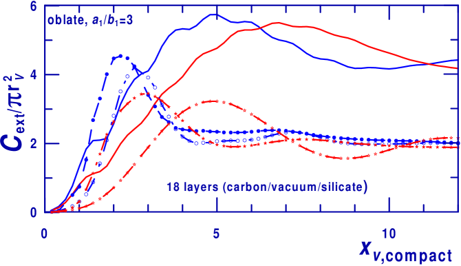
Figure 4: Size dependence of the normalized extinction cross sections for 18-layered prolate and oblate spheroids with $a_{1}/b_{1}=3$. Particles contain an equal fraction of carbon and silicate without vacuum (the porosity ${\cal P}=0.0$) or 50% of vacuum (the porosity ${\cal P}=0.50$). For a given value of the size parameter, the compact and porous particles have the same mass. The cyclic order of the different material layers is: carbon/vacuum/silicate (starting from the core). The effect of the increase of particle porosity and oblique incidence is illustrated.

The difference in the optical properties of compact and porous particles is clearly seen in Fig. 4 which shows the size dependence of normalized cross sections as given by Eqs. (67), (68). The compact and porous particles have the same mass for the same size parameter. This means that variations of the extinction are related to the changes in the particle shape, orientation, porosity, and the particle type (prolate or oblate). As follows from Fig. 4, the position of the first maximum shifts to larger size parameters with a growth of porosity. For very large particles, the normalized cross sections of compact and porous particles cease to fluctuate and become rather similar.

The role of porosity in dust optics can be properly analyzed by using the normalized cross sections

$$C^{\rm(n)}=\frac{C({\rm porous\,grain})}{C({\rm compact\,grain\,of\,same\,mass\,and\,shape})}$$

$$\,\,\,\,\,\,\,=(1-{\cal P})^{-2/3}\,\frac{Q({\rm porous\,grain})}{Q({\rm compact\,grain\,of\,same\,mass\,and\,shape})}.$$ (78)

The quantity $C^{\rm(n)}$ shows how porosity can increase or decrease the cross section. Such an investigation was performed in [22, 23] for spherical particles.

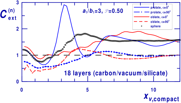
Figure 5: The normalized extinction cross sections (see Eq. (78)) for layered prolate and oblate spheroids with $a_{1}/b_{1}=3$. For $\alpha=90\hbox{${}^{\circ}$}$, the curves are plotted for the sum of the TM and TE modes. The effect of variation of particle type and orientation is illustrated.

Figures 5, 6 show the extinction cross sections $C^{\rm(n)}$ computed for prolate and oblate spheroids with porosity ${\cal P}=0.33$ and 0.5. It is seen that the behavior of curves $C^{\rm(n)}(x_{\rm compact})$ is rather complicated. The porosity increases the extinction for spheroids of almost all sizes and shapes that are seen pole-on ($\alpha=0\hbox{${}^{\circ}$}$) and decreases the extinction for spheroids that are seen edge-on ($\alpha=90\hbox{${}^{\circ}$}$), if $x_{V,{\rm compact}}\mathrel{\mathchoice{\vbox{\offinterlineskip\halign{\hfil$\displaystyle#$\hfil\cr<\cr\sim\cr}}}{\vbox{\offinterlineskip\halign{\hfil$\textstyle#$\hfil\cr<\cr\sim\cr}}}{\vbox{\offinterlineskip\halign{\hfil$\scriptstyle#$\hfil\cr<\cr\sim\cr}}}{\vbox{\offinterlineskip\halign{\hfil$\scriptscriptstyle#$\hfil\cr<\cr\sim\cr}}}}3-5$. Note that in the last case the curves are plotted for the sum of the TM and TE modes for non-polarized incident radiation. For very large particles, the normalized cross sections tends to approach to asymptotic values $C^{\rm(n)}\rightarrow(1-{\cal P})^{-2/3}$ (see Eq. (78)) which are equal to 1.31 and 1.59 if ${\cal P}=0.33$ and 0.5, respectively.

7 Conclusions

The main results of the paper are as follows:

1. We have solved the light scattering problem for a confocal multilayered spheroid by using the extended boundary condition method (EBCM) with a corresponding spheroidal basis. Our recursive solution is based on a special choice of scalar potentials which for any next layer can be found by using the potentials of the previous layer, the procedure starting from the particle core.

2. The numerical code has been thoroughly examined by using various tests. They have demonstrated that the convergence of the efficiency factors for multilayered spheroids is not a function of layers number $N$ and is independent of particle shape. These features make our solution with a spheroidal basis essentially different from the SVM or EBCM approach with spherical basis. Our code allows one to calculate the optical properties of spheroids with the size parameters up to $x_{V}=2\pi r_{V}/\lambda\approx 15-20$ ($r_{V}$ is the radius of equivolume sphere) including very elongated or flattened particles.

3. Illustrative calculations show the convergence of the extinction factors to average values with a growing number of layers. In the case of the large number of layers, the optical properties of layered particles slightly depend on the order of the materials and are determined by the volume fraction of the materials. Variations of extinction with a growth of particle porosity demonstrate increase of the extinction for spheroids of almost all sizes and shapes that are seen pole-on ($\alpha=0\hbox{${}^{\circ}$}$) and decrease of the extinction for spheroids that are seen edge-on ($\alpha=90\hbox{${}^{\circ}$}$), if $x_{V,{\rm compact}}\mathrel{\mathchoice{\vbox{\offinterlineskip\halign{\hfil$\displaystyle#$\hfil\cr<\cr\sim\cr}}}{\vbox{\offinterlineskip\halign{\hfil$\textstyle#$\hfil\cr<\cr\sim\cr}}}{\vbox{\offinterlineskip\halign{\hfil$\scriptstyle#$\hfil\cr<\cr\sim\cr}}}{\vbox{\offinterlineskip\halign{\hfil$\scriptscriptstyle#$\hfil\cr<\cr\sim\cr}}}}3-5$.

List of Table Captions

Table 1. Efficiency factors for Extinction $Q_{\rm ext}$ and Scattering $Q_{\rm sca}$ for Prolate and Oblate Multilayered Spheroids at $\alpha=0^{\circ}$.

Table 1: Efficiency factors for Extinction $Q_{\rm ext}$ and Scattering $Q_{\rm sca}$ for Prolate and Oblate Multilayered Spheroids at $\alpha=0^{\circ}$ ^a

	Prolate spheroid						Oblate spheroid
	$a_{1}/b_{1}$ = 2			$a_{1}/b_{1}$ = 10			$a_{1}/b_{1}$ = 2			$a_{1}/b_{1}$ = 10
$N_{\max}$	$Q_{\rm ext}$	$Q_{\rm sca}$		$Q_{\rm ext}$	$Q_{\rm sca}$		$Q_{\rm ext}$	$Q_{\rm sca}$		$Q_{\rm ext}$	$Q_{\rm sca}$
6	7.3	7.9		0.35	0.41		2.30	2.26		0.26	0.23
8	7.40	7.36		0.330	0.332		2.409	2.413		0.252	0.251
10	7.386	7.387		0.3267	0.3264		2.4108	2.4105		0.2544	0.2542
12	7.38691	7.38688		0.32680	0.32679		2.410809	2.410812		0.25426	0.25427
14	7.3869017	7.3869022		0.3268027	0.3268029		2.4108093	2.4108092		0.254276	0.254275
16	7.38690174	7.38690174		0.326802788	0.326802792		2.410809320	2.410809320		0.25427511	0.25427512
18	7.38690174	7.38690174		0.3268027850	0.3268027850		2.4108093212	2.4108093212		0.2542751277	0.2542751273

^a the number of layers $N=18$, ${m}_{j}=1.3+0.0i$, $j=1,4,7,10,13,16$; ${m}_{j}=1.5+0.0i$, $j=2,5,8,11,14,17$; ${m}_{j}=1.7+0.0i$, $j=3,6,9,12,15,18$; $2\pi a_{1}/\lambda=5$, and $V_{j}/V_{\rm total}=1/18$.

List of Figure Captions

Fig. 1. Scattering geometry for a prolate spheroid with the confocal layered structure and $a_{1}/b_{1}=2$. The space is divided into $N+1$ parts: the outer medium (1), the outermost layer (2), $\cdots$, the core ($N+1$). The scattered field in the far-field zone is represented in the spherical coordinate system $(r,\vartheta,\varphi)$. $\Theta$ is the scattering angle. The origin of the Cartesian coordinate system is at the center of the spheroid while the z axis coincides with its axis of revolution. The angle of incidence $\alpha$ is the angle between the direction of incidence and the z axis in the x – z plane.

Fig. 2. Percent difference between three-layered spheres and three-layered spheroids $\epsilon$ defined by Eq. (76): ${m}_{3}=1.7+0.0i$, ${m}_{2}=1.5+0.0i$, ${m}_{1}=1.3+0.0i$, $V_{j}/V_{\rm total}=0.33$, $a_{1}/b_{1}=1.0001$, $\alpha=0\hbox{${}^{\circ}$}$, ($\bullet$) – prolate spheroids, ($\circ$) – oblate spheroids.

Fig. 3. Size dependence of the extinction efficiency factors for layered prolate spheroids with $a_{1}/b_{1}=3$. Each particle contains an equal fraction of carbon, silicate, and vacuum (the porosity ${\cal P}=1/3$) separated in equivolume confocal layers. The cyclic order of the different material layers is indicated (starting from the core). The effect of the increase of the number of layers is illustrated.

Fig. 4. Size dependence of the normalized extinction cross sections for 18-layered prolate and oblate spheroids with $a_{1}/b_{1}=3$. Particles contain an equal fraction of carbon and silicate without vacuum (the porosity ${\cal P}=0.0$) or 50% of vacuum (the porosity ${\cal P}=0.50$). For a given value of the size parameter, the compact and porous particles have the same mass. The cyclic order of the different material layers is: carbon/vacuum/silicate (starting from the core). The effect of the increase of particle porosity and oblique incidence is illustrated.

Fig. 5. The normalized extinction cross sections (see Eq. (78)) for layered prolate and oblate spheroids with $a_{1}/b_{1}=3$. For $\alpha=90\hbox{${}^{\circ}$}$, the curves are plotted for the sum of the TM and TE modes. The effect of variation of particle type and orientation is illustrated.

Fig. 6. The normalized extinction cross sections (see Eq. (78)) for layered oblate spheroids. The effect of variation of particle shape is illustrated.

Figure 6: The normalized extinction cross sections (see Eq. (78)) for layered oblate spheroids. The effect of variation of particle shape is illustrated.

References

• [1] V. G. Farafonov, V. B. Il’in, and M. S. Prokopjeva, “Light scattering by multilayered nonspherical particles: a set of methods,” J. Quant. Spectrosc. Rad. Transfer 79–80, 599–626 (2003).
• [2] F. M. Kahnert, “Numerical methods in electromagnetic scattering theory,” J. Quant. Spectrosc. Rad. Transfer 79–80, 775–824 (2003).
• [3] A. Vinokurov, V. Farafonov, and V. Il’in, “Separation of variables method for multilayered nonspherical particles,” J. Quant. Spectrosc. Rad. Transfer 110, 1356–1368 (2009).
• [4] V. G. Farafonov, “A unified approach, using spheroidal functions, for solving the problem of light scattering by a axisymmetric particles,” J. Math. Sci. 175, 698–723 (2011).
• [5] I. Gurwich, M. Kleiman, N. Shiloah, and A. Cohen, “Scattering of electromagnetic radiation by multilayered spheroidal particles: recursive procedure,” \ao39, 470–477 (2000).
• [6] V. G. Farafonov, “New recursive solution to the problem of scattering of electromagnetic radiation by multilayered spheroidal particles,” Opt. Spectrosc. 90, 743–752 (2001).
• [7] I. Gurwich, M. Kleiman, N. Shiloah, and D. Oaknin, “Scattering by an arbitrary multi-layered spheroid: theory and numerical results,” J. Quant. Spectrosc. Rad. Transfer 79–80, 649–660 (2003).
• [8] Y. Han, H. Zhang, and X. Sun, “Scattering of shaped beam by an arbitrarily oriented spheroid having layers with non-confocal boundaries,” \apB 84, 485–492 (2006).
• [9] D. S. Wang, P. W. Barber, “Scattering by inhomogeneous nonspherical objects”, \ao18, 1190–1197 (1979).
• [10] D. Petrov, Y. Shkuratov, E. Zubko, and G. Videen, “Sh-matrices method as applied to scattering by particles with layered structure”, J. Quant. Spectrosc. Rad. Transfer 106, 437–454 (2007).
• [11] A. Doicu, T. Wriedt, and Y. Eremin, Light scattering by systems of particles (Springer, 2006).
• [12] N. V. Voshchinnikov, V. G. Farafonov, G. Videen, and L. S. Ivlev, “Development of the separation of variables method for multi-layered spheroids”, in Proc. of the 9th Conf. on Electromagnetic and Light Scattering by Nonspherical Particles, N. V. Voshchinnikov, ed. (St. Petersburg Univ., 2006), pp. 271–274.
• [13] V. G. Farafonov, N. V. Voshchinnikov, and V. V. Somsikov, “Light scattering by a core-mantle spheroidal particle,” \ao35, 5412–5426 (1996).
• [14] C. Flammer, Spheroidal Wave Functions (Stanford Univ. Press, 1957).
• [15] I. V. Komarov, L. I. Ponomarev, and S. Yu. Slavyanov, Spheroidal and Coulomb Spheroidal Functions (Nauka, 1976).
• [16] V. G. Farafonov and V. B. Il’in, “Single light scattering: computational methods”, in Light Scattering Reviews, A. A. Kokhanovsky, ed. (Springer, 2006) 1, pp. 125–177.
• [17] N. V. Voshchinnikov and V. G. Farafonov, “Optical properties of spheroidal particles”, Astrophys. Space Sci. 204, 19–86 (1993).
• [18] N. V. Voshchinnikov and V. G. Farafonov, “Numerical treatment of spheroidal wave functions,” In: Electromagnetic and Light Scattering by Nonspherical Particles, B. Å. S. Gustafson et al. (eds.), Army Res. Lab., Adelphi, 325–328 (2002).
• [19] N. V. Voshchinnikov and V. G. Farafonov, “Computation of radial prolate spheroidal wave functions using Jáffe’s series expansions”, J. Comp. Math. Math. Phys. 43, 1299–1309 (2003).
• [20] N. V. Voshchinnikov and J. S. Mathis, “Calculating cross sections of composite interstellar grains,” \apj526, 257–264 (1999).
• [21] B. Posselt, V. G. Farafonov, V. B. Il’in, and M. S. Prokopjeva, “Light scattering by multilayered ellipsoidal particles in the quasistatic approximation”, Measurements and Sci. Technol. 13, 256–262 (2002).
• [22] N. V. Voshchinnikov, V. B. Il’in, and Th. Henning, “Modelling the optical properties of composite and porous interstellar grains”, Astronomy and Astrophysics 429, 371–381 (2005).
• [23] E. Krügel and R. Siebenmorgen, “Dust in protostellar cores and stellar disks”, Astronomy and Astrophysics 288, 929–941 (1994).