Deriving reliable fundamental parameters of PMS-rich star clusters affected by differential reddening

Abstract

We present an approach that improves the search for reliable astrophysical parameters (e.g. age, mass, and distance) of differentially-reddened, pre-main sequence-rich star clusters. It involves simulating conditions related to the early-cluster phases, in particular the differential and foreground reddenings, and internal age spread. Given the loose constraints imposed by these factors, the derivation of parameters based only on photometry may be uncertain, especially for the poorly-populated clusters. We consider a wide range of cluster (i) mass and (ii) age, and different values of (iii) distance modulus, (iv) differential and (v) foreground reddenings. Photometric errors and their relation with magnitude are also taken into account. We also investigate how the presence of unresolved binaries affect the derived parameters. For each set of (i) - (v) we build the corresponding model Hess diagram, and compute the root mean squared residual with respect to the observed Hess diagram. The parameters that produce the minimum residuals between model and observed Hess diagrams are searched by exploring the full parameter space of (i) - (v) by means of brute force, which may be time consuming but efficient. Control tests show that an adequate convergence is achieved allowing for solutions with residuals 10% higher than the absolute minimum. Compared to a colour-magnitude diagram containing only single stars, the presence of 100% of unresolved binaries has little effect on cluster age, foreground and differential reddenings; significant differences show up in the cluster mass and distance from the Sun. Our approach shows to be successful in minimising the subjectiveness when deriving fundamental parameters of young star clusters.

1 Introduction

Because of important dynamically-induced structural changes, the first few $10^{7}$ yr represent the most critical period in a star cluster’s life, especially for the low-mass embedded clusters (ECs). At this stage, cluster dissolution is essentially related to the impulsive parental gas removal by supernovae and massive star winds. Following the rapid change in the gravitational potential - and the reduced escape velocity - an important fraction of the stars, even all stars, escape to the field. This process has been shown capable of dissolving most of the very young star clusters on a time-scale of $10-40$ Myr (e.g. Tutukov 1978; Goodwin & Bastian 2006). We point out that, because of gas and dust ejection, young clusters with most of the stars still in the PMS are not necessarily ECs. Examples might be Bochum 1 (Bica, Bonatto & Dutra 2008), Pismis 5 (Bonatto & Bica 2009b), and NGC 4755 (Bonatto et al. 2006).

Current estimates (e.g. Lada & Lada 2003; Bonatto & Bica 2011b) suggest that less than $\sim 5\%$ of the Galactic ECs dynamically evolve into gravitationally bound open clusters (OCs). Thus, such a massive early dissolution of ECs may be an important source of Galactic field stars (e.g. Massey, Johnson & Gioia-Eastwood 1995).

It is in this context that a robust determination of fundamental parameters (e.g. age, distance, mass, reddening, etc) of young star clusters is important. However, several factors severely challenge this task, most of which are related to the conspicuous presence of pre-main sequence (PMS) stars in Colour-Magnitude Diagrams (CMDs) of young, low-mass star clusters. Evolving towards the under-populated MS, the PMS stars are usually shrouded within a non-uniform dust distribution, which may lead to a high degree of differential reddening. Examples of clusters characterised by such CMDs are NGC 6611, NGC 4755, NGC 2244, Bochum 1, Pismis 5, NGC 1931, vdB 80, Cr 197 and vdB 92 (Bonatto & Bica 2009a; Bonatto & Bica 2010a and references therein). This effect is particularly critical for the very young clusters that are still in the (gas and dust) embedded phase. As an additional complicating factor, star formation within a cluster is not characterised by a single event. Instead, stars in young clusters are observed to form over a significant time spread (e.g. Stauffer et al. 1997, and references therein), usually comparable to the cluster age. In summary, CMDs of clusters younger than $\mbox{$t_{age}$}\sim 30-40$ Myr are expected to contain stars with a range of ages ($\leq\mbox{$t_{age}$}$) and affected by varying degrees of differential reddening. And, since most of the stellar mass of a young cluster is stored in the PMS, the combined effect of the age spread and differential reddening complicates the straightforward derivation of cluster fundamental parameters. This is especially true when photometry is the only available information on a cluster.

Given the relevance of the above issues, it’s natural that previous approaches with different sophistication degrees have been developed, exploring similar lines as in the present paper. For instance, Naylor & Jeffries (2006) present a powerful and formally elegant maximum-likelihood method to derive distances and ages of young clusters through comprehensive Hess diagram simulations. Although allowing for the presence of binaries in an isochronal population, their method does not include age spread or differential reddening. Also, it appears to apply more consistently to clusters with CMDs satisfactorily described by a single isochrone, i.e., those without a significant PMS age spread (usually older than $\sim 30$ Myr). Later, da Rio, Gouliermis & Gennaro (2010) improves on the Naylor & Jeffries (2006) method by including differential reddening, age spreads and PMS stars in the simulations. However, distance and reddening are not free parameters in da Rio, Gouliermis & Gennaro (2010); instead, they are adopted from previously estimated values. Hillenbrand, Bauermeister & White (2008) presents another attempt to modelling CMDs of young star clusters by means of varying star formation histories. Based on confusion between signal and noise in CMDs, they conclude that there is only marginal evidence for moderate age spreads in recent star forming regions and young open clusters. More recently, Stead & Hoare (2011) apply a Monte Carlo method to the age determination of embedded clusters through near-infrared (UKIDSS) photometry. They deredden the photometry of a real cluster and compare it with models built from theoretical isochrones.

In this work we simulate some relevant conditions that usually apply to the early cluster phases to approach the problem of obtaining reliable fundamental parameters of PMS-rich clusters affected by varying degrees of differential reddening. We adopt a simplistic approach, keeping the number of assumptions - and free parameters - to a minimum. In short, we start by building a distribution of artificial stars (i.e. with mass and absolute luminosity) corresponding to clusters of a range of masses and ages. Next, we apply a set of values of foreground reddening, distance modulus and differential reddening to the model stars, and build the corresponding Hess diagram. Photometric uncertainties and their smearing effect on CMDs are explicitly taken into account. At each step we compare the artificial and observed Hess diagrams, searching for the set of values that produce the best match. Binaries - in varying fractions - are also included in the simulated Hess diagrams. Formally, our brute-force approach is not as elegant as some of the previous methods (see above). However, it has the advantage of fully exploring the parameter space in the search for the best set of values, although at the cost of heavy computer time when working with fine grids (Sect. 2.2).

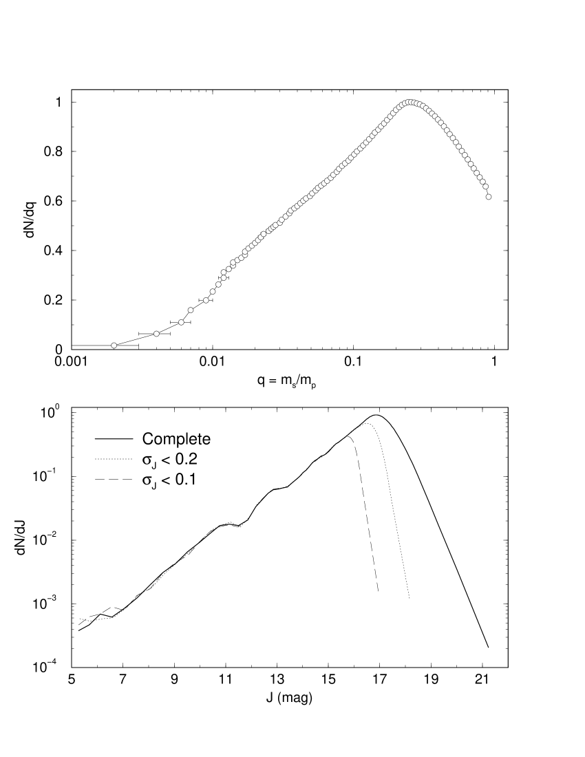
Figure 1: Top: Binary mass-ratio distribution that result from pairing stars with similar ages (and any mass) on a cluster undergoing continuous star formation for 20 Myr. $m_{s}$ and $m_{p}$ are the secondary and primary-star mass, respectively. The distribution’s peak at $q\approx 0.25$ has been normalized to unity. Bottom: $J$-band photometric completeness as a function of different error tolerances (see Sect. 2.2 for details).

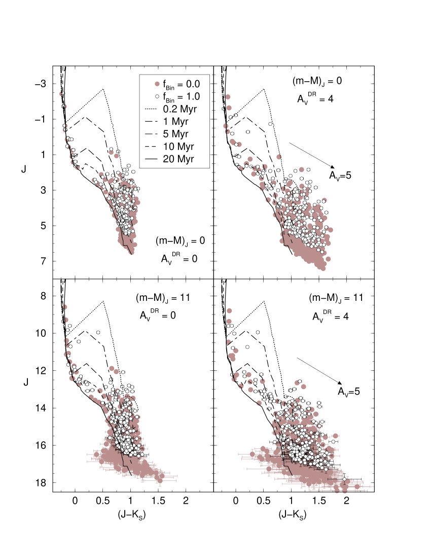
Figure 2: Template CMD of a 20 Myr and 250 $\rm M_{\odot}$ cluster with stars submitted to $\mbox{$A_{V}^{DR}$}=0$ (left panels) and $\mbox{$A_{V}^{DR}$}=4$ (right), displaced at $\mbox{$(m-M)_{J}$}=0$ (top) and $\mbox{$(m-M)_{J}$}=11$ (bottom). The arrow shows the reddening vector for $\mbox{$A_{V}$}=5$. The foreground reddening is zero in all cases. For comparison, evolutionary sequences corresponding to binary fractions of 0% (filled symbols) and 100% (empty) are considered.

The present paper is organised as follows. In Sect. 2 we discuss the relevant effects that affect the CMDs and describe the approach. In Sect. 3 we apply the approach to some control cases and discuss the results in terms of the residual statistics. In Sect. 4 we do the same with two previously studied young clusters. Concluding remarks are given in Sect. 5.

2 Young cluster simulations

For consistency with previous work by our group on young clusters (e.g. Bonatto & Bica 2010a), we consider here photometric properties (e.g. the relationship between errors with apparent magnitude, quality control, CMDs) that usually apply to 2MASS. The all-sky coverage and uniformity of 2MASS, associated with a moderate near-infrared photometric depth, provide an adequate environment for probing properties even of deeply embedded clusters (e.g. Bonatto & Bica 2011a and references therein). For similar reasons, we work with $\mbox{$J$}\times\mbox{$(J-K_{s})$}$ CMDs (this colour is the least affected by photometric errors and the best discriminant for PMS stars - e.g. Bonatto & Bica 2010b) and the corresponding Hess diagrams. Thus, in what follows we refer to the apparent distance modulus as $(m-M)_{J}$, foreground reddening as $E(J-K_{s})$, and differential reddening as $A_{V}^{DR}$. Reddening transformations are based on the absorption relations $A_{J}/A_{V}=0.276$ and $A_{K_{S}}/A_{V}=0.118$, with $R_{V}=3.1$ (Cardelli, Clayton & Mathis 1989; Dutra, Santiago & Bica 2002).

Photometric uncertainties - which are assumed to be Normally distributed - are taken into account when building the Hess diagrams. Formally, if the magnitude (or colour) of a given star is given by $\bar{x}\pm\sigma_{x}$, the probability of finding it at a specific value $x$ is given by $P(x)=\frac{1}{\sqrt{2\pi}\sigma_{x}}\,e^{{-\frac{1}{2}}\left(\frac{x-\bar{x}}{\sigma_{x}}\right)^{2}}$. Thus, for each star we compute the fraction of the magnitude and colour that occurs in a given bin of a Hess diagram, which corresponds to the difference of the error functions computed at the bin borders. By definition, summing the colour and magnitude density over all Hess bins results in the number of input stars. As a compromise between CMD resolution and computational time, the Hess diagrams used in this work consist of magnitude and colour bins of size $\Delta\mbox{$J$}=0.2$ and $\Delta\mbox{$(J-K_{s})$}=0.02$, respectively.

Binary systems are expected to survive the early evolutionary phase of low-mass clusters, with the unresolved pairs being somewhat brighter than the single stars and producing some broadening of the CMD stellar sequences (e.g. Naylor & Jeffries 2006). In addition, binaries also produce changes on the initial mass function of young, massive star clusters (e.g. Weidner, Kroupa & Maschberger 2009). Thus, we also include them in our simulations by means of the parameter $f_{bin}$, which measures the fraction of unresolved binaries in a CMD. According to this definition, a CMD having $N_{CMD}$ detections, but characterised by the binary fraction $f_{bin}$, would have a number of individual stars expressed as $N_{*}=(1+\mbox{$f_{bin}$})N_{CMD}$. For consistency with our assumption of continuous star formation (Sect. 2.2), binaries are formed by pairing stars with the closest ages, regardless of the individual masses. This gives rise to a secondary to primary star mass-ratio ($q=m_{s}/m_{p}$) that smoothly increases from very-low values up to $q\approx 0.25$, and decreases for higher values of $q$ (Fig. 1).

2.1 A first look at the problem

Most of the difficulties associated with obtaining reliable fundamental parameters for young clusters are summarised in Fig. 2, in which we present a template CMD corresponding to a 250 $\rm M_{\odot}$ cluster with an age of 20 Myr, and no foreground reddening. For the stellar mass/luminosity relation we use the solar-metallicity isochrone sets of Padova (Girardi et al. 2002) isochrones and Siess, Dufour & Forestini (2000). Both isochrone sets have been merged for each age considered, since Padova isochrones should be used only for the MS (or more evolved sequences), while those of Siess apply to the PMS. The merging point occurs at the MS, at $6.5\,\mbox{$\rm M_{\odot}$}$ for the isochrones younger than 8 Myr, $5.5\,\mbox{$\rm M_{\odot}$}$ for 10 Myr, $4.5\,\mbox{$\rm M_{\odot}$}$ for 20 Myr, and $3.5\,\mbox{$\rm M_{\odot}$}$ for 30 Myr. The models are built with stars with mass $\geq 0.1\,\mbox{$\rm M_{\odot}$}$, the lowest mass considered in the PMS isochrones.

First we consider zero distance modulus and no differential reddening. At this point the template stars are relatively bright and simply distribute among the isochrones according to the age and mass, with very small photometric uncertainties. When the template stars are displaced by e.g. $\mbox{$(m-M)_{J}$}=11$ (still with no differential reddening), a significant scatter shows up, increasing for fainter stars. Finally, when a moderate value of differential reddening ($\mbox{$A_{V}^{DR}$}=4$) is added to the template, the scatter tends to mask any relationship between stars and isochrones, even for $\mbox{$(m-M)_{J}$}=0$. Clearly, this effect increases with distance modulus. At each step we also show the stellar sequences corresponding to the maximum possible binary fraction, $\mbox{$f_{bin}$}=1.0$. While the mild brightening implied by the binaries with respect to the single stars (Sect. 4) is clearly seen in all cases, the broadening ends up drowned both by the intrinsic PMS age spread and photometric errors. Thus, the binary-related broadening should be more noticeable in the MS of massive clusters of any age.

Note that, as a photometric quality control, we have kept only the stars with $J$ and $K_{s}$ errors lower than 0.5. Such a loose constraint is used here only for illustrative purposes. In what follows we work only stars with errors lower than 0.2. The error restriction is used to somehow emulate the photometric completeness function of the observations. We illustrate this effect on the luminosity function of an artificial cluster containing an arbitrarily large number of stars, for statistical purposes (Fig. 1). After following the steps described below for assigning magnitudes and uncertainties, we applied the restriction of keeping only stars with $\sigma_{J}\leq 0.1$ and 0.2. Compared to the complete luminosity function, which presents a turnover at $\mbox{$J$}\approx 16.9$, the restricted functions have turnovers that smoothly shift towards brighter magnitudes.

2.2 Description of the approach

Briefly put, we start by building the Hess diagram corresponding to the $\mbox{$J$}\times\mbox{$(J-K_{s})$}$ CMD of a young cluster. Then we search - by means of brute force - for the set of values of cluster stellar mass ($M_{clu}$), age ($t_{age}$), differential reddening ($A_{V}^{DR}$), foreground reddening ($E(J-K_{s})$), and apparent distance modulus ($(m-M)_{J}$), that produces the best match between the observed and simulated Hess diagrams. Note that, to minimise the number of free parameters, we assume a uniform (or flat) distribution for the differential reddening. Alternative shapes might be tested, such as a normal distribution around a mean value. However, this would require an additional parameter (the standard deviation), and CMDs of young clusters might lack constraints to find the best values for a large number of free parameters. Also, we assume that for a cluster of age $t_{age}$ and mass $M_{clu}$, stars (of mass $m$) form continuously between $0\leq t\leq\mbox{$t_{age}$}$. In this context, the cluster age also characterises the star-formation time spread, since we assume the cluster age to coincide with the beginning of the star formation. As a caveat we note that assuming a flat age distribution may be somewhat unrealistic, especially for clusters older than $\sim 10$ Myr, since this would imply a very slow and steady star formation rate. However, except for the artificial clusters used as control tests below, in this paper we apply our approach to clusters younger than this threshold.

The approach takes on the following steps: (i) Start with an artificial cluster of mass $M_{clu}$, age $t_{age}$, apparent distance modulus $(m-M)_{J}$, and foreground reddening $E(J-K_{s})$. (ii) Select the stellar masses by randomly taking values from Kroupa (2001) mass function, until the individual mass sum yields $M_{clu}$. (iii) Randomly assign each star an age $\leq\mbox{$t_{age}$}$. (iv) As another simplifying assumption, consider that each star can be randomly absorbed by any value of (differential) reddening in the range $0\leq\mbox{$A_{V}$}\leq\mbox{$A_{V}^{DR}$}$. (v) Apply shifts in colour and magnitude according to the values of $E(J-K_{s})$ and $(m-M)_{J}$. (vi) Assign each artificial star a photometric uncertainty based on the average 2MASS errors and magnitude relationship. (vii) For more realistic representativeness, add some photometric noise to the stars. This step is done to minimise the probability of stars with the same mass having exactly the same observed magnitude, colour, and uncertainty in the CMD. Consider a star (of mass $m$ and age $t_{age}$) with an intrinsic (i.e., measured from the corresponding isochrone) magnitude $mag_{i}$ and assigned uncertainty $\sigma_{mag}$. The noise-added magnitude $mag$ is then randomly computed from a Normal distribution with a mean $mag_{i}$ and standard deviation $\sigma_{mag}$. (viii) Apply the same detection limit to the model CMD as for the observations, so that model and data share a similar photometric completeness function; in practice, this means that stars with photometric errors higher than 0.2 are discarded. (ix) Build the corresponding $\mbox{$J$}\times\mbox{$(J-K_{s})$}$ Hess diagram, compare it with the observed one and compute the root mean squared residual $R_{RMS}$ (see below) for this set of values. (x) Repeat steps (i) - (x) for a range of values of $M_{clu}$, $t_{age}$, $A_{V}^{DR}$, $E(J-K_{s})$, and $(m-M)_{J}$. Finally, analyse the topology of the hyperspace defined by $\mbox{$R_{RMS}$}=\mbox{$R_{RMS}$}(\mbox{$M_{clu}$},\mbox{$t_{age}$},\mbox{$A_{V}^{DR}$},\mbox{$E(J-K_{s})$},\mbox{$(m-M)_{J}$})$ and search for solutions around the minimum values of $R_{RMS}$. Some technical details are described below.

Kroupa (2001) mass function is defined as $dN/dm\propto m^{-(1+\chi)}$, with the slopes $\chi=0.3$ for $0.08\leq m(\mbox{$\rm M_{\odot}$})\leq 0.5$ and $\chi=1.3$ for $m(\mbox{$\rm M_{\odot}$})>0.5$. The relation of errors with magnitude for 2MASS is well represented by $\sigma_{J}=0.0214+2.48\times 10^{-8}\exp{(J/1.071)}$ and $\sigma_{K_{s}}=0.0193+9.59\times 10^{-9}\exp{(K_{s}/1.067)}$. As for the photometric noise for a star with magnitude $mag\pm\sigma_{mag}$, a new magnitude is randomly taken from the Normal distribution characterised by the mean $mag$ and standard deviation $\sigma_{mag}$.

With respect to the root mean squared residual between observed ($H_{obs}$) and simulated ($H_{sim}$) Hess diagrams composed of $n_{c}$ and $n_{m}$ colour and magnitude bins, we define

$$\mbox{$R_{RMS}$}=\sqrt{\sum_{i,j=1}^{n_{c},n_{m}}\frac{\left[H_{obs}(i,j)-H_{sim}(i,j)\right]^{2}}{n_{c}\times n_{m}}}.$$

To minimise the critical stochasticity associated with low-mass clusters, in step (i) we build $N_{sim}$ clusters of mass $M_{clu}$ and age $t_{age}$. To improve the statistical significance, the final simulations, in most cases, are run with $N_{sim}=250$. In this sense, the artificial Hess diagram (step (ix)) corresponds to the average density over the $N_{sim}$ clusters.

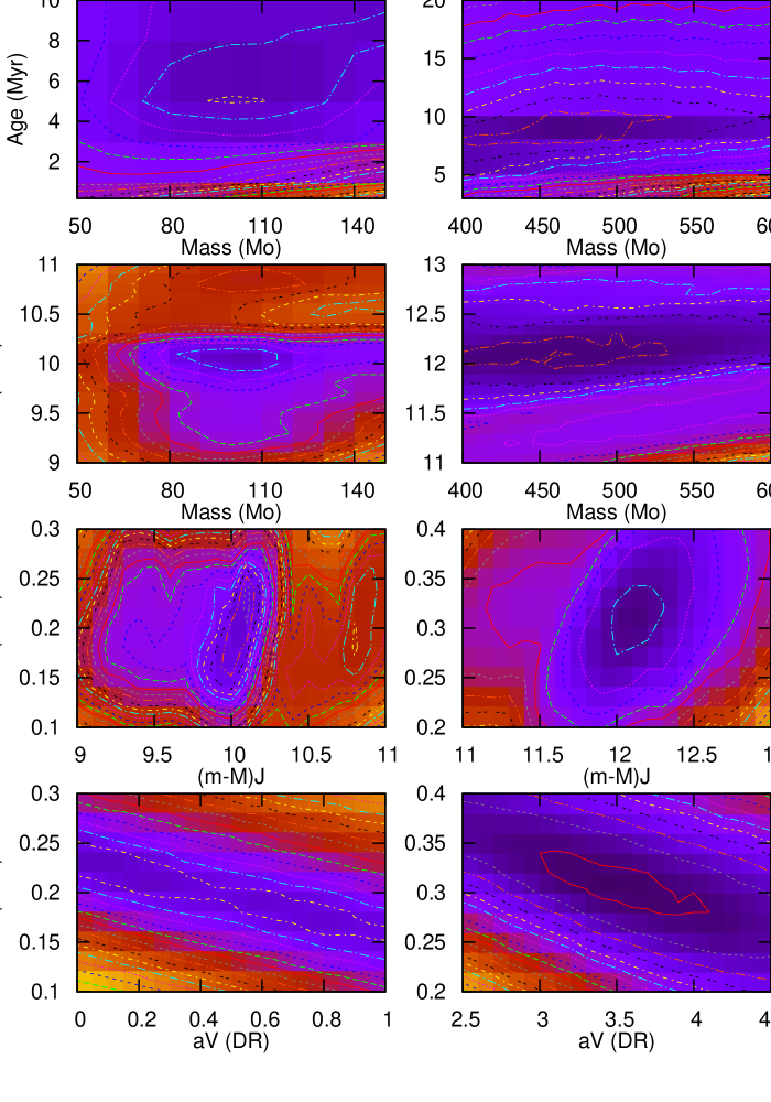
Figure 3: $R_{RMS}$ contour maps for selected parameters of MODEL#2 (left) and MODEL#3 (right). Darker colours indicate lower values of $R_{RMS}$. The absolute minima are $\mbox{$R_{RMS}$}=0.034$ (MODEL#2) and $\mbox{$R_{RMS}$}=0.028$ (MODEL#3).

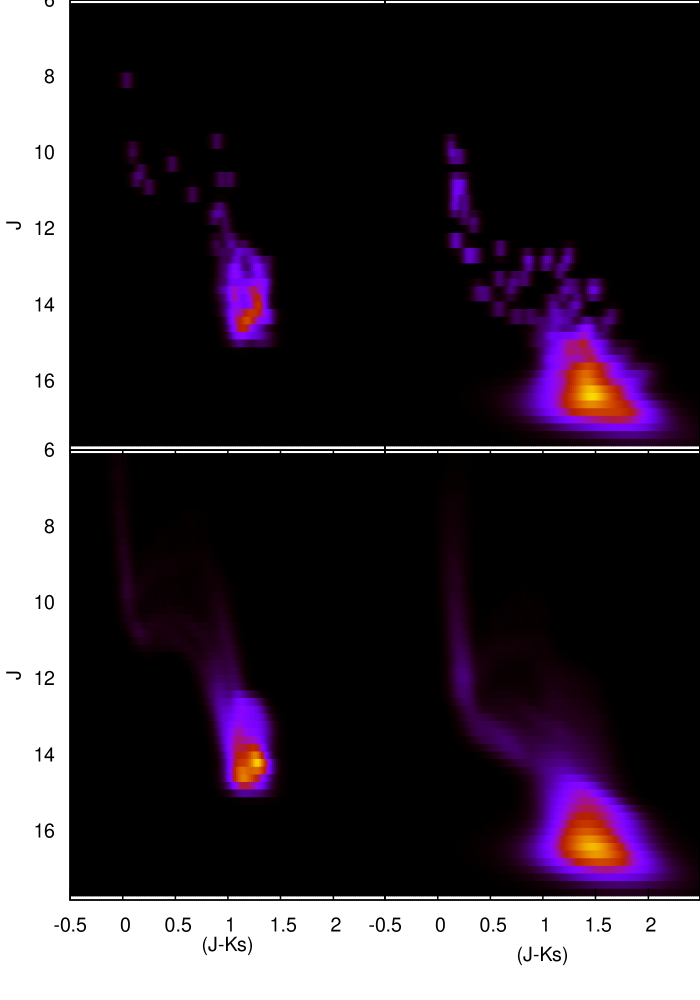
Figure 4: Observed (top panels) and simulated (bottom) Hess diagrams for MODEL#2 (left) and MODEL#3 (right). Lighter colours indicate higher densities of stars. The simulated diagrams have been built with the 10%-higher parameters (Table 1).

For practical reasons, the age grid is restricted to $t_{age}$= 0.2, 1, 3, 5, 8, 10, 20 and 30 Myr. Indeed, as can be inferred from Fig. 2, a finer age grid would be redundant. The stellar mass/luminosity relation is taken from the respective merged set of solar-metallicity Padova and Siess isochrones. Magnitudes for stars with intermediate age values are obtained by interpolation among the neighbouring isochrones. According to the adopted isochrone sets, the minimum stellar mass is 0.1 $\rm M_{\odot}$, while the maximum ranges from 60 $\rm M_{\odot}$ (at 0.2 Myr), 36 $\rm M_{\odot}$ (5 Myr), 19 $\rm M_{\odot}$ (10 Myr), and 9 $\rm M_{\odot}$ (30 Myr).

As described above, the brute-force nature of our approach tends to be very time consuming. For instance, a typical simulation for a cluster with $\sim 500$ stars would require a parameter grid composed (at least) of 21 mass bins, 5 ages, 21 distance moduli, 21 foreground reddenings and 21 differential reddenings. Then, including the $N_{sim}$ clusters in the simulation, the runtime (for the minimum grid) is about 10 hours on a single core of an Intel Core i7 920@2.67 GHz processor.

3 Control experiments

Before turning to actual cases, we apply the approach described above to template CMDs built with typical parameters found in PMS-rich young clusters. The main reason is to examine the ability to recover the input parameters and their relation with the $R_{RMS}$ statistics. The relevant parameters of the adopted models cover the ranges $100\leq\mbox{$M_{clu}$}(\mbox{$\rm M_{\odot}$})\leq 500$, $3\leq\mbox{$t_{age}$}(\rm Myr)\leq 20$, $9.5\leq\mbox{$(m-M)_{J}$}\leq 12$, $0.1\leq\mbox{$E(J-K_{s})$}\leq 0.4$, and $0.5\leq\mbox{$A_{V}^{DR}$}\leq 3.5$. The models are described in Table 1, which also contains quantitative details of the search for solutions on the $R_{RMS}$ maps.

Besides the single solution for the absolute $R_{RMS}$ minimum, we also explore the solutions with $R_{RMS}$ occurring within thresholds 5%, 10%, 25%, and 50% higher than the absolute minimum. For these, the parameters given in Table 1 correspond to the weighted average of all the solutions matching each threshold. As weight for each solution we take the individual value of $1/R^{2}_{RMS}$. Except for a few cases, there’s little difference among the average values of a given model, from the absolute minimum to the 50% threshold. As expected, the most noticeable difference in the output lies in the significantly increasing dispersion around the average for higher thresholds. Although somewhat subjective, we believe that the best convergence is obtained with the 10% threshold (which also produces realistic errors), which is consistent with the somewhat irregular topology of the $R_{RMS}$ maps (see below). Overall, the approach seems very sensitive to the parameters, especially the age and differential reddening. The residual $R_{RMS}$ of the 10%-higher solutions occur in the range $0.023\leq\mbox{$R_{RMS}$}\leq 0.051$. As an additional perspective on the statistical significance of the solutions within the adopted residual thresholds, we also provide in Table 1 the percentage of $N_{sol}$ with respect to the full range of possibilities (which depends on the number of parameter bins). Note that even allowing for the 10%-higher threshold, the fraction of acceptable solutions corresponds to $\sim 1-5\%$ of the total number.

Table 1: Recovery of model fundamental parameters ($N_{sim}=500$; $\mbox{$f_{bin}$}=0.0$)

$R_{RMS}$	Range	$N_{sol}$	$f_{sol}$	$M_{clu}$	Age	$(m-M)_{J}$	$E(J-K_{s})$	$A_{V}^{DR}$	$M_{CMD}$
			(%)	($\rm M_{\odot}$)	(Myr)	(mag)	(mag)	(mag)	($\rm M_{\odot}$)
(1)	(2)	(3)	(4)	(5)	(6)	(7)	(8)	(9)	(10)
Input parameters of MODEL#1				$250$	$3$	$9.5$	$0.1$	$3.0$
$0.0463$	Abs. minimum	1	$1.7\times 10^{-3}$	$240\pm 0$	$3.0\pm 0.0$	$9.60\pm 0.00$	$0.14\pm 0.00$	$2.8\pm 0.0$	$160\pm 0$
$\leq 0.0487$	5% higher	303	$5.1\times 10^{-1}$	$233\pm 11$	$3.0\pm 0.1$	$9.59\pm 0.04$	$0.14\pm 0.02$	$2.8\pm 0.2$	$156\pm 8$
$\leq 0.0510$	10% higher	1030	$1.7$	$235\pm 16$	$3.0\pm 0.1$	$9.58\pm 0.05$	$0.13\pm 0.02$	$2.9\pm 0.2$	$156\pm 10$
$\leq 0.0579$	25% higher	4002	$6.7$	$234\pm 20$	$3.0\pm 0.1$	$9.57\pm 0.08$	$0.13\pm 0.03$	$2.9\pm 0.2$	$155\pm 13$
$\leq 0.0695$	50% higher	9023	$15.0$	$234\pm 21$	$3.0\pm 0.2$	$9.56\pm 0.11$	$0.12\pm 0.03$	$2.9\pm 0.2$	$155\pm 14$
Input parameters of MODEL#2:				$100$	$5$	$10.0$	$0.2$	$0.5$
$0.0336$	Abs. minimum	1	$1.4\times 10^{-3}$	$100\pm 0$	$5.0\pm 0.0$	$10.10\pm 0.00$	$0.22\pm 0.00$	$0.2\pm 0.0$	$106\pm 0$
$\leq 0.0353$	5% higher	214	$3.0\times 10^{-1}$	$104\pm 6$	$5.0\pm 0.1$	$10.08\pm 0.04$	$0.21\pm 0.02$	$0.4\pm 0.2$	$103\pm 6$
$\leq 0.0369$	10% higher	828	$1.2$	$104\pm 9$	$5.0\pm 0.1$	$10.07\pm 0.06$	$0.20\pm 0.02$	$0.5\pm 0.3$	$101\pm 9$
$\leq 0.0420$	25% higher	8977	$13.0$	$108\pm 14$	$6.3\pm 1.5$	$9.95\pm 0.17$	$0.20\pm 0.03$	$0.5\pm 0.3$	$106\pm 14$
$\leq 0.0504$	50% higher	28064	$40.0$	$106\pm 15$	$6.5\pm 1.5$	$9.95\pm 0.19$	$0.21\pm 0.03$	$0.5\pm 0.3$	$103\pm 15$
Input parameters of MODEL#3:				$500$	$10$	$12.0$	$0.3$	$3.5$
$0.0279$	Abs. minimum	1	$5.1\times 10^{-4}$	$495\pm 0$	$8.0\pm 0.0$	$12.20\pm 0.00$	$0.30\pm 0.00$	$3.7\pm 0.0$	$261\pm 0$
$\leq 0.0293$	5% higher	1811	$9.2\times 10^{-1}$	$494\pm 22$	$8.4\pm 0.8$	$12.16\pm 0.09$	$0.31\pm 0.02$	$3.6\pm 0.2$	$265\pm 11$
$\leq 0.0307$	10% higher	5871	$3.0$	$492\pm 23$	$8.8\pm 1.0$	$12.12\pm 0.13$	$0.31\pm 0.02$	$3.6\pm 0.2$	$265\pm 12$
$\leq 0.0349$	25% higher	21327	$11.0$	$490\pm 24$	$8.8\pm 1.2$	$12.11\pm 0.17$	$0.31\pm 0.03$	$3.6\pm 0.2$	$263\pm 13$
$\leq 0.0418$	50% higher	51482	$26.0$	$489\pm 24$	$8.8\pm 1.5$	$12.12\pm 0.20$	$0.30\pm 0.04$	$3.6\pm 0.2$	$263\pm 13$
Input parameters of MODEL#4:				$150$	$20$	$11.0$	$0.4$	$1.5$
$0.0209$	Abs. minimum	1	$6.1\times 10^{-4}$	$120\pm 0$	$20.0\pm 0.0$	$11.10\pm 0.00$	$0.46\pm 0.00$	$1.1\pm 0.0$	$94\pm 0$
$\leq 0.0219$	5% higher	2154	$1.3$	$142\pm 19$	$24.3\pm 4.9$	$11.09\pm 0.06$	$0.44\pm 0.03$	$1.5\pm 0.3$	$102\pm 14$
$\leq 0.0230$	10% higher	8735	$5.3$	$142\pm 20$	$24.5\pm 5.0$	$11.09\pm 0.10$	$0.44\pm 0.03$	$1.5\pm 0.3$	$101\pm 14$
$\leq 0.0261$	25% higher	43299	$26.0$	$138\pm 23$	$24.6\pm 5.5$	$11.07\pm 0.19$	$0.43\pm 0.04$	$1.5\pm 0.3$	$99\pm 16$
$\leq 0.0313$	50% higher	89775	$55.0$	$135\pm 24$	$24.3\pm 6.1$	$11.07\pm 0.22$	$0.42\pm 0.05$	$1.5\pm 0.3$	$97\pm 17$

• Cols. (1) and (2): $R_{RMS}$ value and corresponding range with respect to the absolute minimum; Col. (3): number of solutions occurring within the $R_{RMS}$ range; Col. (4): percentage of $N_{sol}$ with respect to the full range of solutions; Col. (5): actual cluster mass; Col. (9): differential reddening; Col. (10): mass detected in the CMD. $N_{sim}$ is the number of simulated clusters of mass $M_{clu}$ and age $t_{age}$. The average stellar mass of the models is $\overline{m_{*}}\approx 0.6\,\mbox{$\rm M_{\odot}$}$.

Selected two-dimensional projections of $\mbox{$R_{RMS}$}=\mbox{$R_{RMS}$}(\mbox{$M_{clu}$},\mbox{$t_{age}$},\mbox{$A_{V}^{DR}$},\mbox{$E(J-K_{s})$},\mbox{$(m-M)_{J}$})$ are shown in Fig. 3 for MODELS#2 and 3, those that present extreme values of cluster mass and differential reddening. As discussed above, the approach presents conspicuous convergence towards the input values of the age, cluster mass, and apparent distance modulus. However, the $R_{RMS}$ maps present some spread in both foreground and differential reddening values. In particular, there clearly is an anti-correlation between both reddening sources, in the sense that low (or high) foreground reddenings are compensated for by the approach with high (or low) values of differential reddening.

An important information that in principle could be obtained from CMDs is the cluster mass. More specifically, the fraction stored in MS and PMS stars (in this work it means the mass sum for all stars more massive than $\geq 0.1\,\mbox{$\rm M_{\odot}$}$). However, as discussed in Sect. 1, the intrinsic age spread together with the presence of differential reddening, complicate the task of finding the mass of each star in a CMD. Besides, because of limitations inherent to any photometric system (which, in the present work, are simulated by means of the quality criterion (step (viii) in Sect. 2.2), the number of stars that remain detectable in a CMD tends to decrease as the distance modulus increases. Consequently, the same applies to the stellar mass that would be measured in a CMD ($M_{CMD}$) with respect to the actual cluster mass ($M_{clu}$). After derivation of the fundamental parameters, $M_{CMD}$ can be estimated by finding the probable mass for each star in the CMD. This can be done by interpolation (of the observed colour and magnitude of each star) among the nearest isochrones (for instance, Fig. 7), but the final result would depend heavily on the amount of differential reddening, photometric noise, etc. Obviously, the presence of a large fraction of binaries would produce low values of $M_{CMD}$. By construction, the present approach provides directly the actual cluster mass and, since we keep track of the mass (and photometry) of each star that is used in the simulations, we can also compute the mass present in a CMD. Both mass values are given in Table 1. Interestingly, for the range of $(m-M)_{J}$ covered by the models, the actual cluster mass and that present in the CMDs are essentially the same.

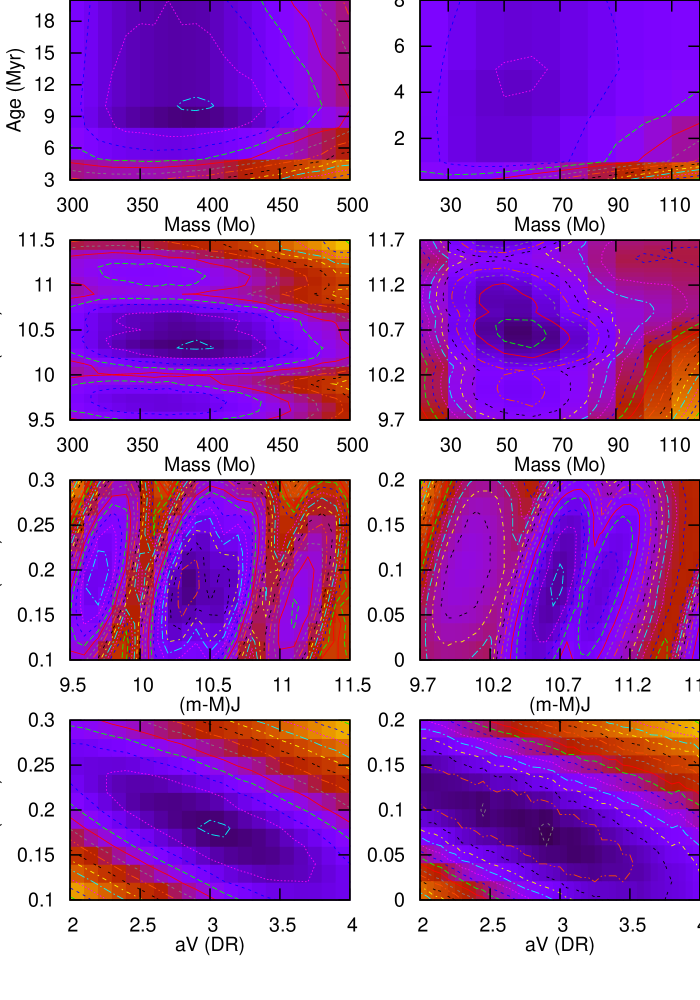
Figure 5: Same as Fig. 3 for the young clusters Collinder 197 (left) and Pismis 5 (right). The absolute minima are $\mbox{$R_{RMS}$}=0.054$ (Collinder 197) and $\mbox{$R_{RMS}$}=0.019$ (Pismis 5).

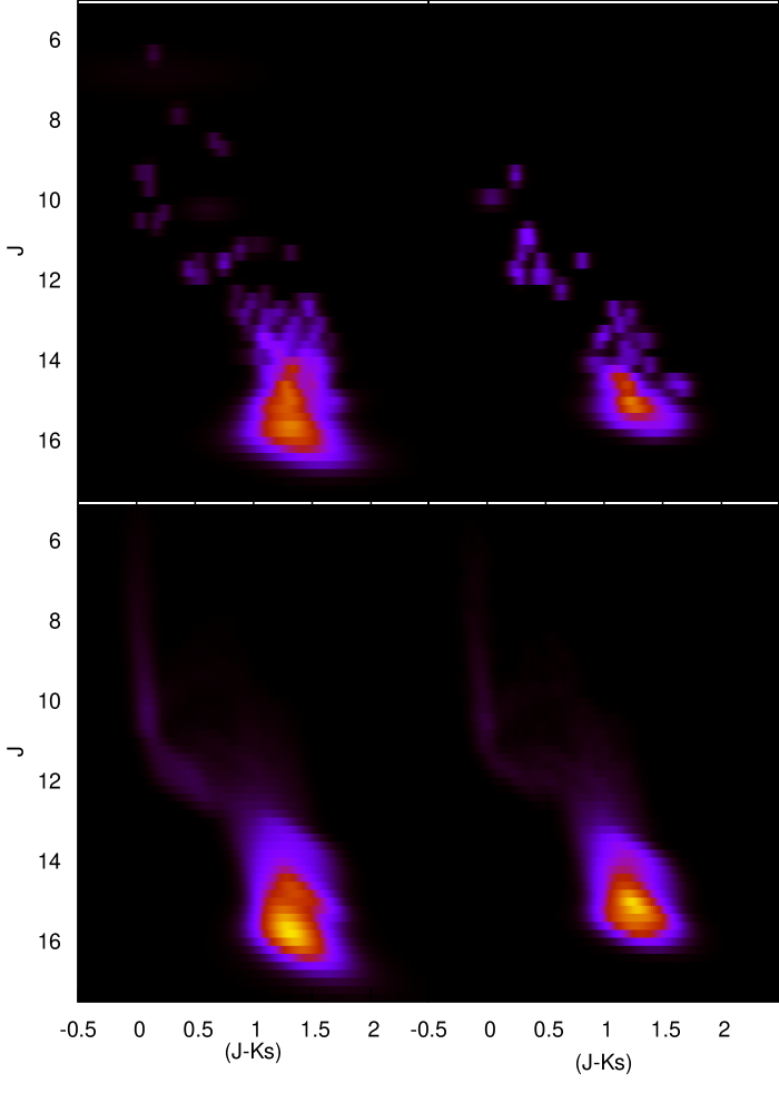
Figure 6: Same as Fig. 4 for the field-star decontaminated (top panels) and simulated (bottom) Hess diagrams of Collinder 197 (left) and Pismis 5 (right).

Another quality assessment criterion is provided by the compared morphology between the model and simulated Hess diagrams (Fig. 4). The latter have been constructed with the parameters found with the 10% threshold (Table 1). Given the low-mass nature of the models considered here, some discreteness in their Hess diagrams is expected. On the other hand, the simulated Hess diagrams correspond to the average over $N_{sim}$ simulated clusters (of mass $M_{clu}$ and age $t_{age}$), and thus, they present a smoother distribution. Nevertheless, model and simulated Hess diagrams present a good correspondence.

Table 2: Fundamental parameters of the young clusters Collinder 197 and Pismis 5

$R_{RMS}$	Range	$N_{sol}$	$f_{sol}$	$M_{clu}$	Age	$(m-M)_{J}$	$E(J-K_{s})$	$A_{V}^{DR}$	$M_{CMD}$	$d_{\odot}$
			(%)	($\rm M_{\odot}$)	(Myr)	(mag)	(mag)	(mag)	($\rm M_{\odot}$)	(kpc)
(1)	(2)	(3)	(4)	(5)	(6)	(7)	(8)	(9)	(10)	(11)
	Collinder 197 ($\mbox{$f_{bin}$}=0.0$)
$0.0546$	Abs. min.	1	$3.6\times 10^{-4}$	$390\pm 0$	$10.0\pm 0.0$	$10.30\pm 0.00$	$0.18\pm 0.00$	$3.1\pm 0.0$	$245\pm 0$	$1.0\pm 0.0$
$\leq 0.0574$	5% higher	186	$6.7\times 10^{-2}$	$392\pm 18$	$9.8\pm 0.6$	$10.37\pm 0.09$	$0.18\pm 0.02$	$3.0\pm 0.2$	$249\pm 11$	$1.0\pm 0.1$
$\leq 0.0601$	10% higher	759	$2.7\times 10^{-1}$	$393\pm 24$	$9.5\pm 0.9$	$10.41\pm 0.12$	$0.18\pm 0.03$	$3.0\pm 0.3$	$248\pm 15$	$1.0\pm 0.1$
$\leq 0.0683$	25% higher	6527	$2.4$	$388\pm 36$	$9.8\pm 2.7$	$10.42\pm 0.22$	$0.18\pm 0.04$	$3.0\pm 0.5$	$245\pm 23$	$1.0\pm 0.1$
$\leq 0.0819$	50% higher	28754	$10.0$	$381\pm 41$	$9.9\pm 4.0$	$10.48\pm 0.35$	$0.18\pm 0.05$	$3.0\pm 0.5$	$241\pm 26$	$1.1\pm 0.2$
	Collinder 197 ($\mbox{$f_{bin}$}=0.5$)
$0.0566$	Abs. min.	1	$2.0\times 10^{-4}$	$660\pm 0$	$10.0\pm 0.0$	$10.80\pm 0.00$	$0.18\pm 0.00$	$3.1\pm 0.0$	$351\pm 0$	$1.2\pm 0.0$
$\leq 0.0595$	5% higher	354	$6.9\times 10^{-2}$	$666\pm 30$	$10.0\pm 0.2$	$10.85\pm 0.07$	$0.19\pm 0.02$	$3.1\pm 0.2$	$354\pm 16$	$1.3\pm 0.1$
$\leq 0.0623$	10% higher	2037	$4.0\times 10^{-1}$	$661\pm 39$	$9.9\pm 2.3$	$10.88\pm 0.21$	$0.19\pm 0.03$	$3.1\pm 0.3$	$354\pm 21$	$1.3\pm 0.1$
$\leq 0.0708$	25% higher	22660	$4.4$	$648\pm 53$	$10.9\pm 4.7$	$10.86\pm 0.42$	$0.19\pm 0.04$	$3.1\pm 0.5$	$347\pm 28$	$1.3\pm 0.2$
$\leq 0.0849$	50% higher	84596	$17.0$	$645\pm 57$	$10.6\pm 5.2$	$10.96\pm 0.49$	$0.19\pm 0.05$	$3.0\pm 0.6$	$345\pm 31$	$1.3\pm 0.3$
	Collinder 197 ($\mbox{$f_{bin}$}=1.0$)
$0.0553$	Abs. min.	1	$2.0\times 10^{-4}$	$820\pm 0$	$10.0\pm 0.0$	$11.20\pm 0.00$	$0.20\pm 0.00$	$3.0\pm 0.0$	$405\pm 0$	$1.5\pm 0.0$
$\leq 0.0580$	5% higher	359	$7.0\times 10^{-2}$	$824\pm 35$	$9.6\pm 0.8$	$11.21\pm 0.11$	$0.19\pm 0.02$	$3.1\pm 0.2$	$404\pm 17$	$1.5\pm 0.1$
$\leq 0.0608$	10% higher	1697	$3.3\times 10^{-1}$	$816\pm 45$	$9.3\pm 1.0$	$11.27\pm 0.14$	$0.19\pm 0.02$	$3.1\pm 0.3$	$402\pm 22$	$1.5\pm 0.1$
$\leq 0.0691$	25% higher	12174	$2.4$	$803\pm 55$	$9.9\pm 3.1$	$11.25\pm 0.27$	$0.19\pm 0.04$	$3.1\pm 0.5$	$395\pm 27$	$1.5\pm 0.2$
$\leq 0.0829$	50% higher	54465	$11.0$	$796\pm 58$	$10.5\pm 4.8$	$11.27\pm 0.45$	$0.20\pm 0.05$	$3.1\pm 0.5$	$390\pm 28$	$1.5\pm 0.3$
	Pismis 5 ($\mbox{$f_{bin}$}=0.0$)
$0.0188$	Abs. min.	1	$3.5\times 10^{-4}$	$60\pm 0$	$5.0\pm 0.0$	$10.75\pm 0.00$	$0.08\pm 0.00$	$2.9\pm 0.0$	$37\pm 0$	$1.3\pm 0.0$
$\leq 0.0197$	5% higher	1301	$4.5\times 10^{-1}$	$61\pm 6$	$5.0\pm 0.1$	$10.75\pm 0.08$	$0.09\pm 0.03$	$2.9\pm 0.3$	$38\pm 4$	$1.3\pm 0.1$
$\leq 0.0207$	10% higher	4816	$1.7$	$62\pm 10$	$5.0\pm 0.9$	$10.79\pm 0.14$	$0.09\pm 0.03$	$2.9\pm 0.3$	$39\pm 6$	$1.3\pm 0.1$
$\leq 0.0235$	25% higher	51006	$18.0$	$68\pm 18$	$5.6\pm 1.9$	$10.88\pm 0.26$	$0.11\pm 0.04$	$2.9\pm 0.3$	$42\pm 11$	$1.4\pm 0.2$
$\leq 0.0282$	50% higher	133571	$46.0$	$67\pm 21$	$5.8\pm 1.9$	$10.90\pm 0.31$	$0.11\pm 0.04$	$2.9\pm 0.3$	$41\pm 13$	$1.4\pm 0.2$
	Pismis 5 ($\mbox{$f_{bin}$}=0.5$)
$0.0176$	Abs. min.	1	$3.8\times 10^{-4}$	$110\pm 0$	$4.0\pm 0.0$	$11.75\pm 0.00$	$0.10\pm 0.00$	$3.0\pm 0.0$	$57\pm 0$	$2.1\pm 0.0$
$\leq 0.0185$	5% higher	1395	$5.3\times 10^{-1}$	$111\pm 8$	$4.0\pm 0.2$	$11.80\pm 0.09$	$0.10\pm 0.02$	$3.0\pm 0.3$	$58\pm 4$	$2.1\pm 0.1$
$\leq 0.0194$	10% higher	6156	$2.3$	$110\pm 13$	$3.7\pm 0.7$	$11.89\pm 0.23$	$0.10\pm 0.03$	$3.1\pm 0.3$	$56\pm 6$	$2.2\pm 0.2$
$\leq 0.0220$	25% higher	52449	$20.0$	$119\pm 22$	$4.6\pm 1.4$	$11.82\pm 0.29$	$0.11\pm 0.04$	$3.1\pm 0.3$	$62\pm 11$	$2.1\pm 0.3$
$\leq 0.0264$	50% higher	140800	$54.0$	$121\pm 23$	$5.3\pm 2.0$	$11.82\pm 0.31$	$0.11\pm 0.04$	$3.1\pm 0.3$	$58\pm 11$	$2.1\pm 0.3$
	Pismis 5 ($\mbox{$f_{bin}$}=1.0$)
$0.0189$	Abs. min.	1	$3.2\times 10^{-4}$	$140\pm 0$	$5.0\pm 0.0$	$11.60\pm 0.00$	$0.10\pm 0.00$	$3.1\pm 0.0$	$67\pm 0$	$1.9\pm 0.0$
$\leq 0.0198$	5% higher	4865	$1.6$	$131\pm 14$	$4.3\pm 1.0$	$11.74\pm 0.20$	$0.10\pm 0.02$	$3.1\pm 0.3$	$62\pm 7$	$2.0\pm 0.2$
$\leq 0.0208$	10% higher	20900	$6.7$	$131\pm 18$	$4.1\pm 1.0$	$11.81\pm 0.26$	$0.10\pm 0.03$	$3.2\pm 0.3$	$62\pm 9$	$2.1\pm 0.3$
$\leq 0.0236$	25% higher	95284	$30.0$	$134\pm 23$	$4.6\pm 1.7$	$11.84\pm 0.32$	$0.11\pm 0.04$	$3.2\pm 0.3$	$63\pm 11$	$2.1\pm 0.3$
$\leq 0.0283$	50% higher	183790	$59.0$	$132\pm 24$	$4.9\pm 2.0$	$11.88\pm 0.34$	$0.11\pm 0.04$	$3.2\pm 0.3$	$61\pm 11$	$2.2\pm 0.3$

• Collinder 197 presents 690 stars in the CMD, while Pismis 5 shows only 101. Collinder 197 was analysed with $N_{sim}=250$ simulated clusters and, for equivalent statistical results, Pismis 5 was analysed with $N_{sim}=1000$. $f_{bin}$ is the binary fraction. The average stellar mass of the model clusters is $\overline{m_{*}}\approx 0.6\,\mbox{$\rm M_{\odot}$}$.

4 Application to actual young clusters

Having demonstrated the convergence efficiency of our approach with artificial clusters (Sect. 3), we now move on to examining properties of actual cases. For this we have selected two young clusters previously studied by our group, Collinder 197 (Bonatto & Bica 2010a) and Pismis 5 (Bonatto & Bica 2009b). Both present typical CMDs of young clusters, with the difference that Collinder 197 has about 10 times more stars (essentially PMS) in the CMD than Pismis 5.

To put the results derived in the present paper in context, we provide here a brief explanation of the previous method used by our group to obtain parameters of both clusters. While the procedure used in Bonatto & Bica (2010a) and Bonatto & Bica (2009b) to construct the field-star decontaminated CMDs follows a quantitative approach, the fundamental parameter derivation used in both cases is somewhat subjective, depending essentially on a qualitative assessment of the differential reddening. Specifically, the MS$+$PMS isochrones (for a range of ages) are set to zero distance modulus and foreground reddening, and shifted in magnitude and colour until they produce a satisfactory fit of the blue border (and redwards spread) of the MS and PMS stellar distribution. Since we did not dispose of any quantitative tool to evaluate the differential reddening, we simply assumed it to be equivalent to the size of the reddening vector that matched the colour spread among the lower-PMS sequences. For the (CMD extracted from the) region within $R=10\arcmin$ from the centre of Collinder 197, Bonatto & Bica (2010a) find $\mbox{$t_{age}$}=5\pm 4$ Myr, $\mbox{$(m-M)_{J}$}=10.4\pm 0.4$, $\mbox{$E(J-K_{s})$}=0.17\pm 0.08$, $M_{CMD}\approx 450\pm 100\,\mbox{$\rm M_{\odot}$}$, and the distance from the Sun $\mbox{$d_{\odot}$}=1.1\pm 0.2$ kpc. For $R=6\arcmin$ of Pismis 5, Bonatto & Bica (2009b) find $\mbox{$t_{age}$}=5\pm 4$ Myr, $\mbox{$(m-M)_{J}$}=10.4\pm 0.1$, $\mbox{$E(J-K_{s})$}=0.20\pm 0.02$, and $M_{CMD}\approx 58\pm 8\,\mbox{$\rm M_{\odot}$}$, and $\mbox{$d_{\odot}$}=1.0\pm 0.1$ kpc. The adopted age (and uncertainty) is simply the average (and half the difference) between the youngest and oldest MS$+$PMS isochrones compatible with the CMD morphology. The mass was estimated by multiplying the number of CMD stars by the average stellar mass (based on Kroupa 2001 MF); thus, it represents the CMD mass.

Considering the above features, both clusters are excellent candidates to apply the present approach. Given the low number of stars (101) in the CMD of Pismis 5, we increased the number of simulated clusters to $N_{sim}=1000$ for statistically more significant results. Collinder 197 has 690 stars in the CMD, so, we kept $N_{sim}=250$. For a more comprehensive analysis, we have applied our approach considering the binary fractions $\mbox{$f_{bin}$}=0,~{}0.5$ and $1$. The fundamental parameters obtained with the present approach are given in Table 2.

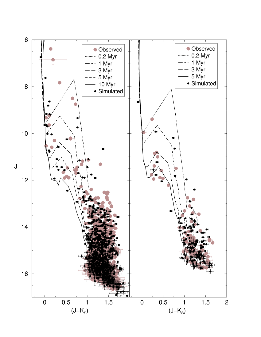
Figure 7: Observed CMDs of Cr 197 (left) and Pismis 5 (right) compared to a single realisation taken from the respective simulations. The extraction radii are 10′ (Cr 197) and 6′ (Pismis 5).

Most of the parameters are essentially insensitive to the presence of unresolved binaries in the CMD. This is especially true for the age, foreground reddening and, to a lesser degree, differential reddening. On the other hand, the most remarkable difference between the presence of (CMD unresolved) binary fractions of 0% and 100% lies in the cluster mass, with $\mbox{$f_{bin}$}=1$ requiring $\approx$ twice more mass than for $\mbox{$f_{bin}$}=0$. Next, the binary-related brightening of the stellar sequences (for $\mbox{$f_{bin}$}=1$) requires an apparent distance modulus, on average, 0.84 and 0.96 higher than for $\mbox{$f_{bin}$}=0$, respectively for Collinder 197 and Pismis 5. This reflects on distances to the Sun $\approx 50\%$ higher if $\mbox{$f_{bin}$}=1$. Within the uncertainties, the parameters corresponding to $\mbox{$f_{bin}$}=0.5$ tend to be closer to those obtained with $\mbox{$f_{bin}$}=1$. Also, for a given binary fraction, the parameters are essentially unchanged with respect to the $R_{RMS}$ ranges considered, although with an increasing dispersion around the average for high $R_{RMS}$. Finally, the convergence level of the approach, as measured by $R_{RMS}$, is essentially the same for the binary fractions considered here. In this sense, our approach appears to be insensitive to the binary fraction, at least for clusters with a significant age spread.

Irrespective of the binary fraction, our results confirm that Pismis 5 is indeed a very-low mass ($\mbox{$M_{clu}$}\sim 60-140\,\mbox{$\rm M_{\odot}$}$) and young ($\mbox{$t_{age}$}\sim 4-6$ Myr) cluster, affected by a moderate amount of differential reddening ($\mbox{$A_{V}^{DR}$}\sim 3.0$), and a low foreground reddening ($\mbox{$A_{V}$}\sim 0.6$). Such a low $A_{V}$, together with the moderate apparent distance modulus ($\mbox{$(m-M)_{J}$}\sim 10.8$, for $\mbox{$f_{bin}$}=0$), puts Pismis 5 at a distance from the Sun of $\mbox{$d_{\odot}$}=1.3\pm 0.1$ kpc. However, this distance may be significantly higher ($\mbox{$d_{\odot}$}=2.1\pm 0.3$ kpc) if $\mbox{$f_{bin}$}=1$.

As anticipated, Collinder 197 is more massive ($\mbox{$M_{clu}$}\sim 390-820\,\mbox{$\rm M_{\odot}$}$) and somewhat older ($\mbox{$t_{age}$}\sim 9.5$ Myr) than Pismis 5, also with a similar value of differential reddening ($\mbox{$A_{V}^{DR}$}\sim 3.0$), and a somewhat higher foreground reddening ($\mbox{$A_{V}$}\sim 1.2$). The distance moduli $\mbox{$(m-M)_{J}$}\sim 10.4$ ($\mbox{$f_{bin}$}=0$) and $\mbox{$(m-M)_{J}$}\sim 11.3$ ($\mbox{$f_{bin}$}=1$) imply the distances $\mbox{$d_{\odot}$}=1.0\pm 0.1$ kpc and $\mbox{$d_{\odot}$}=1.5\pm 0.1$ kpc, respectively. Under the assumptions adopted in Sect. 2.2, the star-formation age spread of Collinder 197 is about twice that of Pismis 5. Interestingly, despite the subjectiveness of the (previous) qualitative assessment we applied to Collinder 197 and Pismis 5, the results of both methods are somewhat compatible, within the uncertainties.

The $R_{RMS}$ projections of Collinder 197 and Pismis 5 (Fig. 5) present similar convergence patterns as those of the control tests (Fig. 3), including the foreground and differential reddening anti-correlation. The residual $R_{RMS}$ of the 10%-higher solutions of Pismis 5 ($\mbox{$R_{RMS}$}\leq 0.021$) is even lower than those of the control tests, and somewhat higher ($\mbox{$R_{RMS}$}\leq 0.06$) for Collinder 197. However, we point out that part of this may be linked to the fact that Collinder 197 has $\approx 7$ times more stars in the CMD, which can result in a larger sum of the residuals. Next, considering the low number of free parameters used by our approach, the observed and simulated Hess diagrams (Fig. 6) present a satisfactory correspondence. Finally, in Fig. 7 we compare a single CMD realisation - randomly selected among the $N_{sim}$ simulated clusters - with the observed CMDs. Having in mind the fact that both are low-mass, young clusters, some differences are more evident because of the low number of stars, especially in the MS, when an isolated, random CMD is used to illustrate the simulations. This effect should be particularly noticeable in poorly-populated clusters, such as Pismis 5. Nevertheless, simulated and observed CMDs are similar, in both cases.

5 Summary and conclusions

In this paper we describe an approach based on CMDs and near-infrared photometry to obtain more accurate fundamental parameters of young star clusters. However, since the presence of large fractions of circumstellar disks around PMS stars can lead to significant excesses in the near-infrared (e.g. Meyer, Calvet & Hillenbrand 1997), the applicability of our approach may be restricted to clusters older than $\sim 3$ Myr (e.g. Haisch, Lada & Lada 2001). Given its statistical nature, our method should be very efficient for well populated clusters, which give rise to smoother stellar-density distributions in the Hess diagrams. But more interestingly, it is expected to work also with the low-mass clusters with CMDs dominated by PMS stars and significantly affected by differential reddening. Among these parameters, cluster mass and age are important to understand the dynamical state (e.g. Bonatto & Bica 2005) of clusters, especially those undergoing the rapidly changing and potentially-destructive evolutionary phase characterised by the first few $10^{7}$ yr.

The approach involves simulating the effect of (random) differential reddening on MS and PMS stars, and its observable results on CMDs. In this paper we apply it to CMDs of star clusters simulated in the 2MASS photometric system. Obviously, it can be adapted to any photometric system, provided isochrones for low-mass stars and very young ages are available.

Beginning with a given cluster mass ($M_{clu}$) and age ($t_{age}$), we distribute the individual stellar masses and magnitudes according to the Kroupa (2001) MF and an MS$+$PMS isochrone set. Subsequently, we build the corresponding simulated Hess diagram for different values of the apparent distance modulus ($(m-M)_{J}$), differential ($A_{V}^{DR}$) and foreground ($E(J-K_{s})$) reddening values. We repeat this for a range of cluster mass and age, searching for the best match between the simulated and observed Hess diagrams. The best-match parameters are searched around the minima of the hypersurface defined by the root mean squared residual $\mbox{$R_{RMS}$}=\mbox{$R_{RMS}$}(\mbox{$M_{clu}$},\mbox{$t_{age}$},\mbox{$A_{V}^{DR}$},\mbox{$E(J-K_{s})$},\mbox{$(m-M)_{J}$})$.

Tests with model clusters containing parameters typical of objects undergoing such an early phase have shown that the present tool converges to the input values, especially when one allows for solutions that occur with $R_{RMS}$ 10% higher than the absolute minimum. We also investigate how unresolved binaries affect the derived parameters. Compared to a CMD containing only single stars, even assuming a presence of 100% of unresolved binaries has little effect (to within the uncertainties) on cluster age, foreground and differential reddenings. Significant differences occur in the cluster mass and distance from the Sun. About twice more mass (in individual stars) is required for $\mbox{$f_{bin}$}=1$ than for $\mbox{$f_{bin}$}=0$, and because of the relative brightening due to the binaries, the distance from the Sun is $\approx 50\%$ larger for $\mbox{$f_{bin}$}=1$ than for $\mbox{$f_{bin}$}=0$.

As a caveat we note that we consider here a particular isochrone set. Thus, the results of our approach tend to be model dependent, since different isochrone sets may lead to different values of mass and age of individual stars (e.g. Hillenbrand, Bauermeister & White 2008) and, consequently, star clusters. In addition, we minimise the number of free parameters by assuming uniform (or flat) distributions of differential reddening and stellar age. Both conditions may be partly unrealistic, especially the latter for clusters older than $\sim 10$ Myr, since it would imply a slow and steady star formation rate. However, the clusters we use here to test the approach, Collinder 197 and Pismis 5, are younger than $\sim 10$ Myr. The relative low-mass nature of both clusters may imply CMDs lacking constraints to find the best values for a large number of free parameters.

The general conclusion is that the inclusion in the simulations of several effects that affect the CMD morphology - especially the differential reddening - produces constrained values of the fundamental parameters. Thus, when photometry is the only available information, our approach minimises the subjectiveness associated with the parameter derivation of young clusters.

References

- Bica, Bonatto & Dutra (2008) Bica E., Bonatto C. & Dutra C.M. 2008, A&A, 489, 1129
- Bonatto & Bica (2005) Bonatto C. & Bica E. 2005, A&A, 437, 483
- Bonatto, Santos Jr. & Bica (2006) Bonatto C., Santos Jr. J.F.C. & Bica E. 2006, A&A, 445, 567
- Bonatto et al. (2006) Bonatto C., Bica E., Ortolani S. & Barbuy B. 2006, A&A, 453, 121
- Bonatto & Bica (2009a) Bonatto C. & Bica E. 2009a, MNRAS, 394, 2127
- Bonatto & Bica (2009b) Bonatto C. & Bica E. 2009b, MNRAS, 397, 1915
- Bonatto & Bica (2010a) Bonatto C. & Bica E. 2010a, A&A, 516, 81
- Bonatto & Bica (2010b) Bonatto C. & Bica E. 2010b, A&A, 521A, 74
- Bonatto & Bica (2011a) Bonatto C. & Bica E. 2011a, MNRAS, 414, 3769
- Bonatto & Bica (2011b) Bonatto C. & Bica E. 2011b, MNRAS, 415, 2827
- Cardelli, Clayton & Mathis (1989) Cardelli J.A., Clayton G.C. & Mathis, J.S. 1989, ApJ, 345, 245
- Dutra, Santiago & Bica (2002) Dutra C.M., Santiago B.X. & Bica E. 2002, A&A, 383, 219
- Girardi et al. (2002) Girardi L., Bertelli G., Bressan A., Chiosi C., Groenewegen M.A.T., Marigo P., Salasnich B. & Weiss A. 2002, A&A, 391, 195
- Goodwin & Bastian (2006) Goodwin S.P. & Bastian N. 2006, MNRAS, 373, 752
- Haisch, Lada & Lada (2001) Haisch K.E. Jr., Lada E.A. & Lada C.J. 2001, ApJL, 553, 153
- Hillenbrand, Bauermeister & White (2008) Hillenbrand L.A., Bauermeister A. & White R.J. 2008, in 14th Cambridge Workshop on Cool Stars, Stellar Systems, and the Sun, ASP Conference Series, Vol. 384, proceedings of the conference held 5-10 November, 2006, at the Spitzer Science Center and Michelson Science Center, Pasadena, California, USA. Edited by Gerard van Belle., p.200
- Kroupa (2001) Kroupa P. 2001, MNRAS, 322, 231
- Lada & Lada (2003) Lada C.J. & Lada E.A. 2003, ARA&A, 41, 57
- Massey, Johnson & Gioia-Eastwood (1995) Massey P., Johnson K.E. & De Gioia-Eastwood K. 1995, ApJ, 454, 151
- Meyer, Calvet & Hillenbrand (1997) Meyer M.R., Calvet N. & Hillenbrand L.A. 1997, AJ, 114, 288
- Naylor & Jeffries (2006) Naylor T. & Jeffries R.D. 2006, MNRAS, 373, 1251
- da Rio, Gouliermis & Gennaro (2010) da Rio N., Gouliermis D.A. & Gennaro M. 2010, ApJ, 723, 166
- Siess, Dufour & Forestini (2000) Siess L., Dufour E. & Forestini M. 2000, A&A, 358, 593
- Skrutskie et al. (2006) Skrutskie M.F., Cutri R., Stiening R., Weinberg M.D., Schneider S.E., Carpenter J.M., Beichman C., Capps R. et al. 2006, AJ, 131, 1163
- Stauffer et al. (1997) Stauffer J.R., Hartmann L.W., Prosser C.F., Randich S., Balachandran S., Patten B.M., Simon T. & Giampapa M. 1997, ApJ, 479, 776
- Stead & Hoare (2011) Stead J. & Hoare M. 2011, MNRAS, accepted (arXiv:1107.5457)
- Tutukov (1978) Tutukov A.V. 1978, A&A, 70, 57
- Weidner, Kroupa & Maschberger (2009) Weidner C., Kroupa P. & Maschberger T. 2009, MNRAS, 393, 663