Bayesian Optimization for Adaptive MCMC

Abstract

This paper proposes a new randomized strategy for adaptive MCMC using Bayesian optimization. This approach applies to non-differentiable objective functions and trades off exploration and exploitation to reduce the number of potentially costly objective function evaluations. We demonstrate the strategy in the complex setting of sampling from constrained, discrete and densely connected probabilistic graphical models where, for each variation of the problem, one needs to adjust the parameters of the proposal mechanism automatically to ensure efficient mixing of the Markov chains.

1 Introduction

A common line of attack for solving problems in physics, statistics and machine learning is to draw samples from probability distributions $\pi(\cdot)$ that are only known up to a normalizing constant. Markov chain Monte Carlo (MCMC) algorithms are often the preferred method for accomplishing this sampling task, see e.g. Andrieu et al. (2003) and Robert & Casella (1998). Unfortunately, these algorithms typically have parameters that must be tuned in each new situation to obtain reasonable mixing times. These parameters are often tuned by a domain expert in a time-consuming and error-prone manual process. Adaptive MCMC methods have been developed to automatically adjust the parameters of MCMC algorithms. We refer the reader to three recent and excellent comprehensive reviews of the field (Andrieu & Thoms, 2008; Atchade et al., 2009; Roberts & Rosenthal, 2009).

Adaptive MCMC methods based on stochastic approximation have garnered the most interest out of the various adaptive MCMC methods for two reasons. Firstly, they can be shown to be theoretically valid. That is, the Markov chain is made inhomogenous by the dependence of the parameter updates upon the history of the Markov chain, but its ergodicity can be ensured (Andrieu & Robert, 2001; Andrieu & Moulines, 2006; Saksman & Vihola, 2010). For example, Theorem 5 of Roberts & Rosenthal (2007) establishes two simple conditions to ensure ergodicity: (i) the non-adaptive sampler has to be uniformly ergodic and (ii) the level of adaptation must vanish asymptotically. These conditions can be easily satisfied for discrete state spaces and finite adaptation.

Secondly, adaptive MCMC algorithms based on stochastic approximation have been shown to work well in practice (Haario et al., 2001; Roberts & Rosenthal, 2009; Vihola, 2010). However, there are some limitations to the stochastic approximation approach. Some of the most successful samplers rely on knowing either the optimal acceptance rate or the gradient of some objective function of interest. Another disadvantage is that these stochastic approximation methods may require many iterations. This is particularly problematic when the objective function being optimized by the adaptation mechanism is costly to evaluate. Finally, gradient approaches tend to be local and hence they can get trapped in local optima when the Markov chains are run for a finite number of steps in practice.

This paper aims to overcome some of these limitations. It proposes the use of Bayesian optimization (Brochu et al., 2009) to tune the parameters of the Markov chain. The proposed approach, Bayesian-optimized MCMC, has a few advantages over adaptive methods based on stochastic approximation.

Bayesian optimization does not require that the objective function be differentiable. This enables us to be much more flexible in the design of the adaptation mechanisms. We use the area under the auto-correlation function up to a specific lag as the objective function in this paper. This objective has been suggested previously by Andrieu & Robert (2001). However, the computation of gradient estimates for this objective is very involved and far from trivial (Andrieu & Robert, 2001). We believe this is one of the main reasons why practitioners have not embraced this approach. Here, we show that this objective can be easily optimized with Bayesian optimization. We argue that Bayesian optimization endows the designer with greater freedom in the design of adaptive strategies.

Bayesian optimization also has the advantage that it is explicitly designed to trade off exploration and exploitation and is implicitly designed to minimize the number of expensive evaluations of the objective function (Brochu et al., 2009; Lizotte et al., 2011).

Another important property of Bayesian-optimized MCMC is that it does not use a specific setting for the parameters of the proposal distribution, but rather a distribution over parameter settings with probabilities estimated during the adaptation process. Indeed, we find that a randomized policy over a set of parameter settings mixes faster than a specific parameter value for the models considered in this paper.

Bayesian optimization has been used with MCMC in Rasmussen (2003) with the intent of approximating the posterior with a surrogate function to minimize the cost of hybrid Monte Carlo evaluations. The intent in this paper is instead to adapt the parameters of the Markov chain to improve mixing.

To demonstrate MCMC adaptation with Bayesian optimization, we study the problem of adapting a sampler for constrained discrete state spaces proposed recently by Hamze & de Freitas (2010). The sampler uses augmentation of the state space in order to make large moves in discrete state space. In this sense, the sampler is similar to the Hamiltonian (hybrid) Monte Carlo for continuous state spaces (Duane et al., 1987; Neal, 2010). Although these samplers typically only have two parameters, these are very tricky to tune even by experts. Moreover, every time we make a change to the model, the expert is again required to spend time tuning the parameters. This is often the case when dealing with sampling from discrete probabilistic graphical models, where we often want to vary the topology of the graph as part of the data analysis and experimentation process. In the experimental section of this paper, we will discuss several Ising models, also known as Boltzmann machines, and show that indeed the optimal parameters vary significantly for different model topologies.

There are existing consistency results for Bayesian optimization (Vasquez & Bect, 2008; Srinivas et al., 2010; Bull, 2011). These results in combination with the fact that we focus on discrete distributions are sufficient for ensuring ergodicity of our adaptive MCMC scheme under vanishing adaptation. However, the type of Bayesian optimization studied in this paper relies on latent Gaussian processes whose covariance grows as the Markov chain progresses. For very large chains, it becomes prohibitive to invert the covariance matrix of the Gaussian process. Thus, for practical reasons, we adopt instead a two-stage adaptation mechanism, where we first adapt the chain for a finite number of steps and then use the most promising parameter values to run the chain again with a mixture of MCMC kernels (Andrieu & Thoms, 2008). Although this adaptation strategy increases the computational cost of the MCMC algorithm, we argue that this cost is much lower than the cost of having a human in the loop choosing the parameters.

2 Adaptive MCMC

The Metropolis-Hasting (MH) algorithm is the key building block for most MCMC methods (Andrieu et al., 2003). It draws samples from a target distribution $\pi(\cdot)$ by proposing a move from $\mathbf{x}^{(t)}$ to $\mathbf{y}^{(t+1)}$ according to a parameterized proposal distribution $q_{\theta}(\mathbf{y}^{(t+1)}|\mathbf{x}^{(t)})$ and either accepting it ($\mathbf{x}^{(t+1)}=\mathbf{y}^{(t+1)}$) with probability equal to the acceptance ratio

$$\alpha(\mathbf{x}^{(t)}\to\mathbf{y}^{(t+1)}) =\min\left\{\frac{\pi(\mathbf{y}^{(t+1)})q_{\theta}(\mathbf{x}^{(t)}|\mathbf{y}^{(t+1)})}{\pi(\mathbf{x}^{(t)})q_{\theta}(\mathbf{y}^{(t+1)}|\mathbf{x}^{(t)})},1\right\}$$

or rejecting it ($\mathbf{x}^{(t+1)}=\mathbf{x}^{(t)}$) otherwise.

The parameters of the proposal, $\theta\in\boldsymbol{\Theta}\subseteq\mathbb{R}^{d}$, can have a large influence on sampling performance. For example, we will consider constrained discrete probabilistic models in our experiments, where changes to the connectivity patterns among the random variables will require different parameter settings. We would like to have an approach that can adjust these parameters automatically for all possible connectivity patterns.

Several methods have been proposed to adapt MCMC algorithms. Instead of discussing all of these, we refer the reader to the comprehensive reviews of Andrieu & Thoms (2008); Atchade et al. (2009); Roberts & Rosenthal (2009). One can adapt parameters other than those of the proposal distribution in certain situations, but for the sake of simplicity, we focus here on adapting the proposal distribution.

One of the most successful adaptive MCMC algorithms was introduced by Haario et al. (2001) and several extensions were proposed by Andrieu & Thoms (2008). This algorithm is restricted to the adaptation of the multivariate random walk Metropolis algorithm with Gaussian proposals. It is motivated by a theoretical result regarding the optimal covariance matrix of a restrictive version of this sampler (Gelman et al., 1996). This adaptive algorithm belongs to the family of stochastic approximation methods.

Some notation needs to be introduced to briefly describe stochastic approximation, which will also be useful later when we replace the stochastic approximation method with Bayesian optimization. Let $\mathcal{X}_{i}=\{\mathbf{x}^{(t)}\}_{t=1}^{i}$ denote the full set of samples up to iteration $i$ of the MH algorithm and $\mathcal{Y}_{i}=\{\mathbf{y}^{(t)}\}_{t=1}^{i}$ be the corresponding set of proposed samples. $\mathbf{x}^{(0)}$ is the initial sample. We will group these samples into a single variable $\mathcal{M}_{i}=(\mathbf{x}^{(0)},\mathcal{X}_{i},\mathcal{Y}_{i})$. Let $g(\theta)$ be the mean field of the stochastic approximation that may only be observed noisily as $G(\theta_{i},\mathcal{M}_{i})$. When optimizing an objective function $h(\theta)$, this mean field corresponds to the gradient of this objective, that is $g(\theta)=\nabla h(\theta)$. Adaptive MCMC methods based on stochastic approximation typically use the following Robbins-Monro update:

$$\theta_{i+1} =\theta_{i}+\gamma_{i+1}G\left(\theta_{i},\mathcal{M}_{i+1}\right),$$ (1)

where $\gamma_{i+1}$ is the step-size. This recursive estimate converges almost surely to the roots of $g(\theta)$ as $i\rightarrow\infty$ under suitable conditions.

We are concerned with the adaptation of discrete models in this paper. The optimal acceptance rates are unknown. It is also not clear what objective function one should optimize to adjust the parameters of the proposal distribution. One possible choice, as mentioned in the introduction, is to use the auto-correlation function up to a certain lag. Intuitively, this objective function seems to be suitable for the adaptation task because it is used in practice to assess convergence. Unfortunately, it is difficult to obtain efficient estimates of the gradient of this objective (Andrieu & Robert, 2001). To overcome this difficulty, we introduce Bayesian optimization in the following section.

3 Bayesian Optimization for Adaptive MCMC

The proposed adaptive strategy consists of two phases: adaptation and sampling. In the adaptation phase Bayesian optimization is used to construct a randomized policy. In the sampling phase, a mixture of MCMC kernels selected according to the learned randomized policy is used to explore the target distribution. The two phases are discussed in more detail subsequently.

3.1 Adaptation Phase

Our objective function for adaptive MCMC cannot be evaluated analytically. However, noisy observations of its value can be obtained by running the Markov chain for a few steps with a specific choice of parameters $\theta_{i}$. Bayesian optimization in the adaptive MCMC setting proposes a new candidate $\theta_{i+1}$ by approximating the unknown function using the entire history of noisy observations and a prior distribution over functions. The prior distribution used in this paper is a Gaussian process.

The noisy observations are used to obtain the predictive distribution of the Gaussian process. An expected utility function derived in terms of the sufficient statistics of the predictive distribution is optimized to select the next parameter value $\theta_{i+1}$. The overall procedure is shown in Algorithm 1. We refer readers to Brochu et al. (2009) and Lizotte (2008) for in-depth reviews of Bayesian optimization.

Algorithm 1 Adaptive MCMC with Bayesian Opt.

1:  for $i=1,2,\dots,I$  do

2:    Run Markov chain for $L$ steps with parameters $\theta_{i}$.

3:    Use the drawn samples to obtain a noisy evaluation of the objective function: $z_{i}=h(\theta_{i})+\epsilon$.

4:    Augment the data $\mathcal{D}_{1:i}=\{\mathcal{D}_{1:i-1},(\theta_{i},z_{i})\}$.

5:    Update the GP’s sufficient statistics.

6:    Find $\theta_{i+1}$ by optimizing an acquisition function: $\theta_{i+1}=\arg\max_{\theta}u(\theta|\mathcal{D}_{1:i})$.

7:  end for

The unknown objective function $h(\cdot)$ is assumed to be distributed according to a Gaussian process with mean function $m(\cdot)$ and covariance function $k(\cdot,\cdot)$:

$$h(\cdot) \sim GP(m(\cdot),k(\cdot,\cdot)).$$

We adopt a zero mean function $m(\cdot)=0$ and an anisotropic Gaussian covariance that is essentially the popular ARD kernel (Rasmussen & Williams, 2006):

$$k(\theta_{j},\theta_{k}) =\exp\left(-\frac{1}{2}(\theta_{j}-\theta_{k})^{T}\textrm{diag}(\psi)^{-2}(\theta_{j}-\theta_{k})\right)$$

where $\psi\in\mathbb{R}^{d}$ is a vector of hyper-parameters. The Gaussian process is a surrogate model for the true objective, which typically involves intractable expectations with respect to the invariant distribution and the MCMC transition kernels. We describe the objective function used in this work in Section 3.3.

We assume that the noise in the measurements is Gaussian: $z_{i}=h(\theta_{i})+\epsilon$, $\epsilon\sim\mathcal{N}(0,\sigma^{2}_{\eta})$. It is possible to adopt other noise models (Diggle et al., 1998). Our Gaussian process emulator has hyper-parameters $\psi$ and $\sigma_{\eta}$. These hyper-parameters are typically computed by maximizing the likelihood (Rasmussen & Williams, 2006). In Bayesian optimization, we can use Latin hypercube designs to select an initial set of parameters and then proceed to maximize the likelihood of the hyper-parameters iteratively (Ye, 1998; Santner et al., 2003). This is the approach followed in our experiments. However, a good alternative is to use either classical or Bayesian quadrature to integrate out the hyper-parameters (Osborne, 2010).

Let $\mathbf{z}_{1:i}\sim\mathcal{N}(0,\mathbf{K})$ be the $i$ noisy observations of the objective function obtained from previous iterations. (Note that the Markov chain is run for $L$ steps for each discrete iteration $i$. The extra index to indicate this fact has been made implicit to improve readability.) $\mathbf{z}_{1:i}$ and $h_{i+1}$ are jointly multivariate Gaussian:

$$\begin{bmatrix}\mathbf{z}_{1:i}\\ h_{i+1}\end{bmatrix} =\mathcal{N}\left(\mathbf{0},\begin{bmatrix}\mathbf{K}+\sigma^{2}_{\eta}I&\mathbf{k}^{T}\\ \mathbf{k}&k(\theta,\theta)\end{bmatrix}\right),$$

where

$$\mathbf{K} =\begin{bmatrix}k(\theta_{1},\theta_{1})&\ldots&k(\theta_{1},\theta_{i})\\ \vdots&\ddots&\vdots\\ k(\theta_{i},\theta_{1})&\ldots&k(\theta_{i},\theta_{i})\end{bmatrix}$$

and $\mathbf{k}=[k(\theta,\theta_{1})\;\ldots\;k(\theta,\theta_{i})]^{T}.$ All the above assumptions about the form of the prior distribution and observation model are standard and less restrictive than they might appear at first sight. The central assumption is that the objective function is smooth. For objective functions with discontinuities, we need more sophisticated surrogate functions for the cost. We refer readers to Gramacy et al. (2004) and Brochu et al. (2009) for examples.

The predictive distribution for any value $\theta$ follows from the Sherman-Morrison-Woodbury formula, where $\mathcal{D}_{1:i}=(\theta_{1:i},\mathbf{z}_{1:i})$:

$$p(h_{i+1}|\mathcal{D}_{1:i},\theta) =\mathcal{N}(\mu_{i}(\theta),\sigma^{2}_{i}(\theta))$$

$$\mu_{i}(\theta) =\mathbf{k}^{T}(\mathbf{K+\sigma_{\eta}^{2}I})^{-1}\mathbf{z}_{1:i}$$

$$\sigma^{2}_{i}(\theta) =k(\theta,\theta)-\mathbf{k}^{T}(\mathbf{K+\sigma_{\eta}^{2}I})^{-1}\mathbf{k}$$

The next query point $\theta_{i+1}$ is chosen to maximize an acquisition function, $u(\theta|\mathcal{D}_{1:i})$, that trades-off exploration (where $\sigma^{2}_{i}(\theta)$ is large) and exploitation (where $\mu_{i}(\theta)$ is high). We adopt the expected improvement over the best candidate as this acquisition function Schonlau et al. (1998); Brochu et al. (2009). This is a standard acquisition function for which asymptotic rates of convergence have been proved (Bull, 2011). However, we point out that there are a few other reasonable alternatives, such as Thompson sampling (May et al., 2011) and upper confidence bounds (UCB) on regret (Srinivas et al., 2010). A comparison among these options as well as portfolio strategies to combine them appeared recently in (Hoffman et al., 2011). There are several good ways of optimizing the acquisition function, including the method of DIvided RECTangles (DIRECT) of Finkel (2003) and many versions of the projected Newton methods of Bertsekas (1982). We found DIRECT to provide a very efficient solution in our domain. Note that optimizing the acquisition function is much easier than optimizing the original objective function. This is because the acquisition functions can be easily evaluated and differentiated.

3.2 Sampling Phase

The Bayesian optimization phase results in a Gaussian process on the $I$ noisy observations of the performance criterion $\mathbf{z}_{1:I}$, taken at the corresponding locations in parameter space $\theta_{1:I}$. This Gaussian process is used to construct a discrete stochastic policy $p(\theta|\mathbf{z}_{1:I})$ over the parameter space $\boldsymbol{\Theta}$. The Markov chain is run with parameter settings randomly drawn from this policy at each step.

One can synthesize the policy $p(\theta|\mathbf{z}_{1:I})$ in several ways. The simplest is to use the mean of the GP to construct a distribution proportional to $\exp(\mu(\theta))$. This is the so-called Boltzmann policy. We can sample $M$ parameter candidates $\theta_{i}$ according to this distribution. Our final sampler then consists of a mixture of $M$ transition kernels, where each kernel is parameterized by one of the $\theta_{i}$, $i=1,\ldots,M$. The distribution of the samples generated in the sampling phase will approach the target distribution $\pi(\cdot)$ as the number of iterations tends to $\infty$ provided the kernels in this finite mixture are ergodic.

In high dimensions, one reasonable approach would be to use a multi-start optimizer to find maxima of the unnormalized Boltzmann policy and then perform local exploration of the modes with a simple Metropolis algorithm. This is a slight more sophisticated version of what is often referred to as the epsilon greedy policy.

The strategies discussed thus far do not take into account the uncertainty of the GP. A solution is to draw M functions according to the GP and then find he optimizer $\theta_{i}$ of each of these functions. This is the strategy followed in (May et al., 2011) for the case of contextual bandits. Although this strategy works well for low dimensions, it is not clear how it can be easily scaled.

3.3 Objective Function

The auto-correlation $r(l,\mathcal{X})$ of a sequence of $n$ generated samples $\mathcal{X}=\{\mathbf{x}^{(1)},\ldots,\mathbf{x}^{(n)}\}$ as a function of the time lag between them is defined as

$$r(l,\mathcal{X}) \triangleq\frac{1}{(n-l)\delta^{2}}\sum_{t=1}^{n-l}(\mathbf{x}^{(t)}-\bar{\mathbf{x}})^{T}(\mathbf{x}^{(t+l)}-\bar{\mathbf{x}}),$$

where $l$ is the lag and $\bar{\mathbf{x}}$ and $\delta^{2}$ are the mean and the variance of $\mathcal{X}$, respectively.

Faster mixing times are characterized by larger values of $a(l_{\textrm{max}},\mathcal{X})=1-({l_{\textrm{max}}}^{-1})\sum_{l=1}^{l_{\textrm{max}}}|r(l,\mathcal{X})|$. We use this property to construct the criterion for Bayesian optimization as follows. Let $\mathcal{E}_{i}$ be the last $i$ sampled states (the energies in the experimental section). The performance criterion is obtained by taking the average of $a(\cdot)$ over a sliding window within the last $L$ samples, down to a minimum window size of $25$: $\frac{1}{L-25+1}\sum_{i=25}^{L}a(i,\mathcal{E}_{i})$.

4 Application to Constrained Discrete Distributions

The Intracluster Move (IM) sampler was recently proposed to generate samples from notoriously-hard constrained Boltzmann machines in (Hamze & de Freitas, 2010). This sampler has two parameters (one continuous and the other discrete) that the authors state to be difficult to tune. This and the recent growing interest in discrete Boltzmann machines in machine learning motivated us to apply the proposed Bayesian-optimized MCMC method to this problem.

Boltzmann machines are described in Ackley et al. (1985). Let $x_{i}\in\{0,1\}$ denote the $i$-th random variable in the model. The Boltzmann distribution is given by

$$\pi(\mathbf{x}) \triangleq\frac{1}{Z(\beta)}e^{-\beta E(\mathbf{x})},$$ (2)

where $Z(\beta)\triangleq\sum_{\mathbf{x}\in\mathcal{S}}e^{-\beta E(\mathbf{x})}$ is the normalizing constant, $\beta$ is a temperature parameter and $E({\mathbf{x}})\triangleq-\sum_{i,j}x_{i}J_{ij}x_{j}-\sum_{i}b_{i}x_{i}$ is the energy function. Boltzmann machines also have coupling parameters $J$ and $b$ that are assumed to be known.

Let $\mathcal{S}_{n}(\mathbf{c})$ be the subset of the states that are at exactly Hamming distance $n$ away from a reference state $\mathbf{c}$. The distribution $\pi_{n,\mathbf{c}}(\mathbf{x})$ is the restriction of $\pi(\mathbf{x})$ to $\mathcal{S}_{n}(\mathbf{c})$. $\pi_{n,\mathbf{c}}(\mathbf{x})$ has $Z_{n}(\beta,\mathbf{c})\triangleq\sum_{\mathbf{x}\in\mathcal{S}_{n}(\mathbf{c})}e^{-\beta E(\mathbf{x})}$ as its normalizing constant and is defined as

$$\pi_{n,\mathbf{c}}(\mathbf{x}) \triangleq\left\{\begin{array}[]{ll}\frac{1}{Z_{n}(\beta,\mathbf{c})}e^{-\beta E(\mathbf{x})}&\text{if }\mathbf{x}\in\mathcal{S}_{n}(\mathbf{c})\\ 0&\text{otherwise}\end{array}\right.$$ (5)

The rest of the paper makes $\mathbf{c}$ implicit and uses the simplified notation $\mathcal{S}_{n}$, $\pi_{n}(\mathbf{x})$ and $Z_{n}(\beta)$. These constraints on the states are used in statistical physics and in regularized statistical models (Hamze & de Freitas, 2010).

The IM sampler proposes a new state $\mathbf{y}^{(t+1)}\in\mathcal{S}_{n}$ from an original state $\mathbf{x}^{(t)}\in\mathcal{S}_{n}$ using self-avoiding walks (SAWs) and has parameters $\theta=(k,\gamma)$, where $k\in\mathcal{L}\triangleq\{1,2,\ldots,k_{\max}\}$ is the length of each SAW and $\gamma\in\mathcal{G}\triangleq[0,\gamma_{\max}]$ is the energy-biasing parameter. $k$ determines the size, in terms of the number of bits flipped, of the moves through $\mathcal{S}_{n}$. $\gamma$ controls the degree to which higher energy states are favored.

4.1 Experimental Setup

The experiments compare the performance of four different sampling methods on three different models. The sampling methods are all instances of the IM sampler that only differ in the manner that $\gamma$ and $k$ are picked:

Kawasaki sampler

: It transitions from state to state within $\mathcal{S}_{n}$ by uniformly sampling a bit to flip to produce a state in $\mathcal{S}_{n+1}$ or $\mathcal{S}_{n-1}$ and then uniformly sampling a bit to flip to return to $\mathcal{S}_{n}$ (Kawasaki, 1966). This is equivalent to running the IM sampler with $\gamma$ fixed to 0 and $k$ fixed to 1.

IMExpert

is the IM sampler manually tuned by a domain expert (Hamze & de Freitas, 2010). The expert set $\gamma$ to a fixed value $\gamma_{\textrm{expert}}$ and $k$ is drawn uniformly in the set $\mathcal{L}$.

IMUnif

is a completely naive approach that draws $\gamma$ uniformly from $\mathcal{G}$ and $k$ uniformly from $\mathcal{L}$.

IMBayesOpt

is the Bayesian-optimized IM with ${L=100}$ samples generated for each of the $100$ adaptations of the parameters.

The algorithm parameters for each model, defined subsequently, are shown in Table 1, where “Others” refers to IMUnif and IMBayesOpt. These two samplers have the same parameter sets because IMUnif is a baseline algorithm used to ensure that Bayesian-optimized IM performs better than a naive strategy.

Table 1: Algorithm parameters and sets for each model following (Hamze & de Freitas, 2010)

MODEL	ALGORITHM	$\mathcal{L}$	$\mathcal{G}$
2DGrid	IMExpert	$\{90\}$	$\{0.44\}$
2DGrid	Others	$\{1,\ldots,300\}$	$[0,0.88]$
3DCube	IMExpert	$\{1,\ldots,25\}$	$\{0.8\}$
3DCube	Others	$\{1,\ldots,50\}$	$[0,1.6]$
RBM	IMExpert	$\{1,\ldots,20\}$	$\{0.8\}$
RBM	Others	$\{1,\ldots,50\}$	$[0,1.6]$

The parameters for IMUnif and IMBayesOpt were selected such that $\mathcal{L}$ is a much larger superset of the SAW lengths used for IMExpert and $\mathcal{G}$ is the contiguous interval from $0$ to $2\gamma_{\textrm{expert}}$. The parameters for IMExpert come from (Hamze & de Freitas, 2010). The Kawasaki sampler does not have any parameters.

Table 2: Model parameters from Hamze & de Freitas (2010). $n$ refers to the number of bits that are set to $1$ out of the total number of bits. $\beta^{-1}$ is the temperature.

MODEL	$\beta^{-1}$	SIZE	$n$
2DGrid	$2.27$	$60\times 60$	$1800$ of $3600$
3DCube	$1.0$	$9\times 9\times 9$	$364$ of $729$
RBM	$1.0$	$|v|=784$, $|h|=500$	$428$ of $1284$

We consider the three models studied by Hamze & de Freitas (2010). The model parameters are given in Table 2. Note that $n$ refers to the Hamming distance from states in $\mathcal{S}_{n}$ to the reference state $\mathbf{c}$. The reference state $\mathbf{c}$ was set to the ground state where none of the bits are set to $1$. This is particularly intuitive in machine learning applications, where we might not want more than a small percentage of the binary variables on as part of a regularization or variable selection strategy.

Ferromagnetic 2D grid Ising model:

The ferromagnetic 2D grid Ising model is made up of nodes arranged in a planar and rectangular grid with connections between the nodes on one boundary to the nodes on the other boundary for each dimension (i.e. periodic boundaries), also known as a square toroidal grid. Hence, each node has exactly four neighbours. The interaction weights, $J_{ij}$, are all 1 and the biases, $b_{i}$, are all 0. The temperature 2.27 is the critical temperature of the model.

Frustrated 3D cube Ising model:

The frustrated 3D cube Ising model is made up of nodes arranged in a topology that is the three-dimensional analogue of the two-dimensional grid with periodic boundaries. Hence, each node has exactly six neighbours. The interaction weights, $J_{ij}$, are uniformly sampled from the set $\{-1,1\}$ and the biases, $b_{i}$, are all 0.

Restricted Boltzmann machine (RBM):

The RBM has a bipartite graph structure, with $h$ hidden nodes in one partition and $v$ visible nodes in the other. The interaction weights $J_{ij}$ and biases $b_{i}$ are exactly the same as in Hamze & de Freitas (2010) and correspond to local Gabor-like filters that capture regularities in perceptual inputs.

Each sampler was run five times with $9\times 10^{4}$ steps for each run. IMBayesOpt had an additional $10^{4}$ steps for an adaptation phase consisting of $100$ adaptations of $100$ samples each. IMBayesOpt was not penalized for the computational overhead involved in these additional steps because it is seen as being far cheaper than having the IM sampler parameters tuned manually.

Figure 1: [Left] Mean and error bars of the auto-correlation function of the energies of the sampled states drawn from the 2D grid Ising model. [Right] Average of the energies.

Figure 2: [Left] The mean function of the Gaussian processes over $\boldsymbol{\Theta}$, learned by IMBayesOpt for the 2D grid Ising model. An average over the five trials is shown. [Right] The corresponding policy used for sampling.

All of the algorithms have a burn-in phase consisting of the first $10^{4}$ samples generated in the corresponding sampling phase. The burn-in phase was not included in the computation of the auto-correlation functions in figures 1, 3 and 5.

IMBayesOpt begins its sampling phase in the same starting state as all of the other samplers, even though it would most likely be in a low energy state at the end of its adaptation phase. This ensures that the comparison of the sampling methods is fair.

4.2 Results

4.2.1 Ferromagnetic 2D grid Ising model

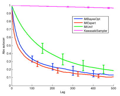
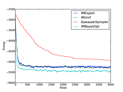
IMExpert and IMBayesOpt both have very similar mean ACFs, as indicated in figure 1. IMUnif suffers from many long strings of consecutive proposal rejections. This is evident from the many intervals where the sampled state energy does not change.

Figure 3: [Left] Mean and error bars of the auto-correlation function of the energies of the sampled states drawn from the 3D cube Ising model. [Right] Average of the energies.

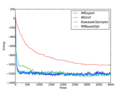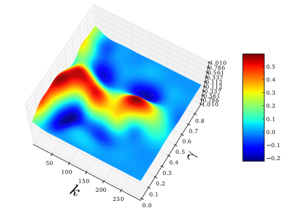
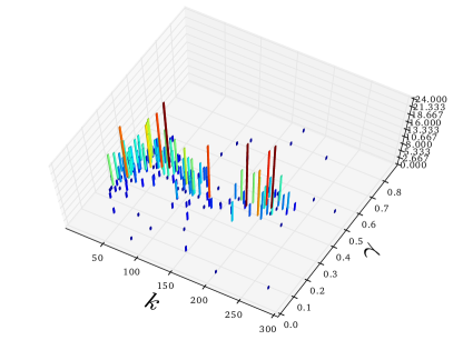
Figure 2 suggests that $\gamma$ is much more important to the performance of the IM sampler than the SAW lengths for this model, especially at large SAW lengths. One of the highest probability points in the Gaussian process corresponds to the parameters chosen by Hamze & de Freitas (2010) $(\gamma=0.44,k=90)$. Figure 2 also shows $M=1000$ samples drawn from the Boltzmann policy. The MCMC results are for this policy. The same procedure is adopted for the other models.

4.2.2 Frustrated 3D cube Ising model

Figure 3 shows that IMUnif now performs far worse than the IMExpert and IMBayesOpt, implying that the extremely rugged energy landscape of the 3D cube Ising model makes manual tuning a non-trivial and necessary process. IMBayesOpt performs very similarly to IMExpert, but is automatically tuned without any human intervention.

Figure 4: [Left] The mean function of the Gaussian processes over $\boldsymbol{\Theta}$, learned by IMBayesOpt for the 3D cube Ising model. An average over the five trials is shown. [Right] The corresponding policy used for sampling.

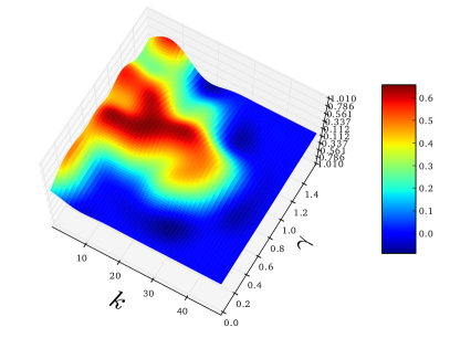
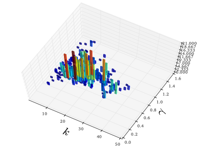
The Gaussian process mean function in Figure 4 suggests that SAW lengths should not be longer than $k=25$, as found in Hamze & de Freitas (2010). Both IMExpert and IMBayesOpt are essentially following the same strategy and performing well, while the performance of IMUnif confirms that tuning is important for the 3D cube Ising model.

4.2.3 Restricted Boltzmann Machine (RBM)

Figure 5: [Left] Mean and error bars of the auto-correlation function of the energies of the sampled states drawn from the 3D cube Ising model. [Right] Average of the energies.

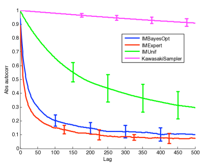
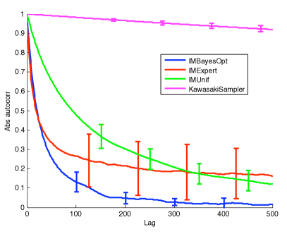
Hamze & de Freitas (2010) find that IMExpert experiences a rapid dropoff in ACF, but this dropoff is exaggerated by the inclusion of the burn-in phase. Figure 5 shows a much more modest dropoff when the burn-in phase is left out of the ACF computation. However, it still corroborates the claim in Hamze & de Freitas (2010) that IMExpert performs far better than the Kawasaki sampler.

Figure 6: [Left] The mean function of the Gaussian processes over $\boldsymbol{\Theta}$, learned by IMBayesOpt for the RBM. An average over the five trials is shown. [Right] The corresponding policy used for sampling.

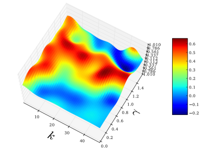
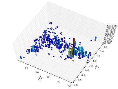
Figure 5 shows that IMExpert does not perform much better than IMUnif. The variance of IMExpert’s ACF is also much higher than any of the other methods. IMBayesOpt performs significantly better than any of the other methods, including manual tuning by a domain expert.

The Gaussian process mean function in figure 6 suggests that SAW lengths greater than 20 can be used and are as effective as shorter ones, whereas Hamze & de Freitas (2010) only pick SAW lengths between $1$ and $20$. This discrepancy is an instance where Bayesian-optimized MCMC has found better parameters than a domain expert.

5 Conclusions

Experiments were conducted to assess Bayesian optimization for adaptive MCMC. Hamze & de Freitas (2010) state that it is easiest to manually tune the 2D grid Ising model and that tuning the 3D cube Ising model is more challenging. Manual tuning significantly improves the performance of the IM sampler for these cases, but Bayesian-optimized MCMC is able to realize the same gains without any human intervention. This automatic approach surpasses the human expert for the RBM model.

Bayesian optimization is a general method for adapting the parameters of any MCMC algorithm. It has some advantages over stochastic approximation, as discussed in this paper. However, it presently only applies to parameter spaces of up to fifty dimensions. Bayesian optimization should not be seen as a replacement for stochastic approximation, but rather as a complementary technique. In particular, Bayesian optimization should be adopted when the objective is non-differentiable or expensive to evaluate.

References

- Ackley et al. (1985) Ackley, David H., Hinton, Geoffrey E., and Sejnowski, Terrence J. A learning algorithm for Boltzmann machines. Cognitive Science, 9:147–169, 1985.
- Andrieu & Moulines (2006) Andrieu, Christophe and Moulines, Eric. On the ergodicity properties of some adaptive MCMC algorithms. The Annals of Applied Probability, 16(3):1462–1505, 2006.
- Andrieu & Robert (2001) Andrieu, Christophe and Robert, Christian. Controlled MCMC for optimal sampling. Technical Report 0125, Cahiers de Mathematiques du Ceremade, Universite Paris-Dauphine, 2001.
- Andrieu & Thoms (2008) Andrieu, Christophe and Thoms, Johannes. A tutorial on adaptive MCMC. Statistics and Computing, 18(4):343–373, 2008.
- Andrieu et al. (2003) Andrieu, Christophe, de Freitas, Nando, Doucet, Arnaud, and Jordan, Michael I. An Introduction to MCMC for Machine Learning. Machine Learning, 50(1):5–43, January 2003.
- Atchade et al. (2009) Atchade, Yves, Gersende Fort, Eric Moulines, and Priouret, Pierre. Adaptive Markov chain Monte Carlo: Theory and methods. Technical report, University of Michigan, 2009.
- Bertsekas (1982) Bertsekas, Dimitri P. Projected Newton methods for optimization problems with simple constraints. SIAM J. on Control and Optimization, 20(2):221–246, 1982.
- Brochu et al. (2009) Brochu, Eric, Cora, Vlad M., and de Freitas, Nando. A tutorial on Bayesian optimization of expensive cost functions, with application to active user modeling and hierarchical reinforcement learning. Technical Report TR-2009-23, Department of Computer Science, University of British Columbia, November 2009.
- Bull (2011) Bull, Adam D. Convergence rates of efficient global optimization algorithms. Arxiv preprint arXiv:1101.3501, 2011.
- Diggle et al. (1998) Diggle, P. J., Tawn, J. A., and Moyeed, R. A. Model-based geostatistics. Journal of the Royal Statistical Society. Series C (Applied Statistics), 47(3):299–350, 1998.
- Duane et al. (1987) Duane, Simon, Kennedy, A. D., Pendleton, Brian J., and Roweth, Duncan. Hybrid Monte Carlo. Physics letters B, 195(2):216–222, 1987.
- Finkel (2003) Finkel, Daniel E. DIRECT Optimization Algorithm User Guide. 2003.
- Gelman et al. (1996) Gelman, Andrew, Roberts, Gareth O., and Gilks, Walter R. Efficient Metropolis jumping rules. In Bernado, J. M. et al. (eds.), Bayesian Statistics, volume 5, pp. 599. OUP, 1996.
- Gramacy et al. (2004) Gramacy, Robert B., Lee, Herbert K. H., and Macready, William G. Parameter space exploration with Gaussian process trees. In International Conference on Machine Learning, pp. 45–52, 2004.
- Haario et al. (2001) Haario, Heikki, Saksman, Eero, and Tamminen, Johanna. An adaptive Metropolis algorithm. Bernoulli, 7(2):223–242, 2001.
- Hamze & de Freitas (2010) Hamze, Firas and de Freitas, Nando. Intracluster moves for constrained discrete-space MCMC. In Uncertainty in Artificial Intelligence, 2010.
- Hoffman et al. (2011) Hoffman, Matt, Brochu, Eric, and de Freitas, Nando. Portfolio allocation for Bayesian optimization. In Uncertainty in Artificial Intelligence, 2011.
- Kawasaki (1966) Kawasaki, Kyozi. Diffusion constants near the critical point for time-dependent Ising models. i. Phys. Rev., 145(1):224–230, 1966.
- Lizotte (2008) Lizotte, Daniel. Practical Bayesian Optimization. PhD thesis, University of Alberta, Edmonton, Alberta, Canada, 2008.
- Lizotte et al. (2011) Lizotte, Daniel, Greiner, Russell, and Schuurmans, Dale. An experimental methodology for response surface optimization methods. Journal of Global Optimization, pp. 1–38, 2011.
- May et al. (2011) May, Benedict C, Korda, Nathan, Lee, Anthony, and Leslie, David S. Optimistic Bayesian sampling in contextual bandit problems. 2011.
- Neal (2010) Neal, Radford M. MCMC using Hamiltonian dynamics. Handbook of Markov Chain Monte Carlo, 2010.
- Osborne (2010) Osborne, Michael. Bayesian Gaussian Processes for Sequential Prediction, Optimisation and Quadrature. PhD thesis, University of Oxford, Oxford, UK, 2010.
- Rasmussen & Williams (2006) Rasmussen, Carl E. and Williams, Christopher. Gaussian Processes for Machine Learning. MIT Press, 2006.
- Rasmussen (2003) Rasmussen, Carl Edward. Gaussian processes to speed up hybrid Monte Carlo for expensive Bayesian integrals. Bayesian Statistics, 7:651–659, 2003.
- Robert & Casella (1998) Robert, Christian P. and Casella, George. Monte Carlo Statistical Methods. Springer, 1st edition, 1998.
- Roberts & Rosenthal (2007) Roberts, Gareth O. and Rosenthal, Jeffrey S. Coupling and ergodicity of adaptive Markov chain Monte Carlo algorithms. Journal of applied probability, 44(2):458–475, 2007.
- Roberts & Rosenthal (2009) Roberts, Gareth O. and Rosenthal, Jeffrey S. Examples of adaptive MCMC. Journal of Computational and Graphical Statistics, 18(2):349–367, 2009.
- Saksman & Vihola (2010) Saksman, Eero and Vihola, Matti. On the ergodicity of the adaptive Metropolis algorithm on unbounded domains. Annals of Applied Probability, 20(6):2178 – 2203, 2010.
- Santner et al. (2003) Santner, T J, Williams, B, and Notz, W. The Design and Analysis of Computer Experiments. Springer, 2003.
- Schonlau et al. (1998) Schonlau, Matthias, Welch, William J., and Jones, Donald R. Global versus local search in constrained optimization of computer models. Lecture Notes-Monograph Series, 34:11–25, 1998.
- Srinivas et al. (2010) Srinivas, Niranjan, Krause, Andreas, Kakade, Sham M, and Seeger, Matthias. Gaussian process optimization in the bandit setting: No regret and experimental design. In Proc. International Conference on Machine Learning (ICML), 2010.
- Vasquez & Bect (2008) Vasquez, Emmanuel and Bect, Julien. On the convergence of the expected improvement algorithm. Technical Report arXiv:0712.3744v2, arXiv.org, Feb 2008.
- Vihola (2010) Vihola, Matti. Grapham: Graphical models with adaptive random walk Metropolis algorithms. Computational Statistics and Data Analysis, 54(1):49 – 54, 2010.
- Ye (1998) Ye, Kenny Q. Orthogonal column Latin hypercubes and their application in computer experiments. Journal of the American Statistical Association, 93(444):1430–1439, 1998.