Hexagonal Warping Effects on the Surface Transport in Topological Insulators

Abstract

We investigate the charge conductivity and current-induced spin polarization on the surface state of a three-dimensional topological insulator by including the hexagonal warping effect of Fermi surface both in classical and quantum diffusion regimes. We present general expressions of conductivity and spin polarization, which are reduced to simple forms for usual scattering potential. Due to the hexagonal warping, the conductivity and spin polarization show an additional quadratic carrier density dependence both for Boltzmann contribution and quantum correction. In the presence of warping term, the surface states still reveal weak anti-localization. Moreover, the dielectric function in the random phase approximation is also explored, and we find that it may be momentum-angle-dependent.

I introduction

Topological insulator (TI) has been attracting a great deal of research both experimentally and theoretically in the past few yearsKane2005 ; qi2008 ; qi2010topological due to its potential applications in topological quantum computationFu2008 and spintronics.Garate2010 A TI has a full energy gap in bulk, while there are gapless surface states stable against weak disorder and weak interaction unless time-reversal symmetry is broken.Wu2006helical ; xu2006stability In particular, the number of its Dirac points is odd according to a no-go theorem,Wu2006helical in vivid contrast to the graphene.novoselov2005two Hence, many theoretical studies focus on a class of TI where the surface states only consist of one Dirac cone.

Experimentally, the surface state has been well confirmed by angle-resolved photoemission spectroscopy (ARPES).hsieh2008topological ; Hsieh13022009 ; Chen10072009 However, the transport observation of surface state in classical diffusion regime meets an obstacle due to the large bulk-conduction background. Recently, Checkelsky et al. claimed to have isolated the surface band contribution in Bi₂Se₃ by electrostatic gate control of chemical potential.checkelsky2010surface Nevertheless, this work is questionable for the reason that the chemical potential is still in the bulk conduction band.Dimitrie Theoretically, D. Culcer et al. investigated the two-dimensional surface charge transport and obtained results analogous to the ones of graphene.Dimitrie Recently, Kim et al. showed that the surface of thin Bi₂Se₃ were electrostatically coupled, strongly.Kim They observed the surface transport by using a gate electrode to remove bulk charge carriers, completely, and well demonstrated the theoretical prediction.Dimitrie It is very likely that this experiment has overcome the above obstacle. Also, the surface anomalous Hall conductivity in TI was calculated using quantum Liouville equation.culcer2010anomalous The electron-phonon scattering limited conductivity was investigated for the surface state of a strong TI.giraud2011electron Moreover, the transverse magnetic heat transport was explored on the topological surface.yokoyama2011transverse

On the other hand, recently, the quantum corrections to charge conductivity in topological surface states were also extensively studied.checkelsky2010surface ; Chen2010 ; HongTao2011 ; Minhao2011 ; lu2011competing ; tkachov2011weak The surface states in quantum diffusion regime ($l_{\phi}\gg l$) reveal positive weak localization correction, i.e. weak anti-localization, which is related to the $\pi$ Berry phase.lu2011competing Here, $l$ and $l_{\phi}$ are the elastic scattering length and the phase coherence length, respectively. In contrast to graphene, where the weak anti-localization is suppressed by the intervalley scattering,McCann2006 the surface states of TI forbid this scattering process due to single Dirac cone and many observations have confirmed this enhancement to electronic conductivity.checkelsky2010surface ; Chen2010 ; HongTao2011 ; Minhao2011 Lu et al. found that the surface state of a TI shows a competing effect of weak localization and weak anti-localization in quantum transport due to magnetic doping.lu2011competing

We have noted that, in most of these theoretical studies, only $\bm{k}$-linear term in the spin-orbit interaction is present in the effective Hamiltonian. However, in some TIs, for example Bi₂Te₃, it was found that the shape of Fermi surface changes from a circle to a hexagon, and then to a snowflake-like shape with increasing the Fermi energy by ARPESChen10072009 and scanning tunneling microscopyZhanybek2010 measurement. With the help of a hexagonal warping term, this kind of band structure was explained by Fu.Fu266801 Note that the states near the Fermi surface are responsible for the transport properties at low temperature. Hence, it is expected that the warping effect will naturally play significant roles on surface transport when the Fermi energy is high enough. So far, only one theoretical work involves the warping effect on the weak anti-localization in the literature.tkachov2011weak Further, they simply replaced the warping term by its angle average one, hence, the anisotropy of energy spectrum due to warping is neglected, completely. Then they acquired the same form of correction as the usual two-dimensional electron gas with spin-orbital interaction. Consequently, it is highly desirable to carefully study the warping effect on the classical contribution and quantum correction to the surface transport.

In this paper, we study the hexagonal warping effect on the charge conductivity and current-induced spin polarization (CISP) in the surface state of a three-dimensional TI. Considering nonmagnetic and magnetic elastic carrier-impurity scattering, we discuss this problem both in classical and quantum diffusive regimes. We also investigate the warping effect on the dielectric function in the random phase approximation (RPA). The structure of the paper is as follows. In Sec. II, the effective Hamiltonian of the surface state is given. By using a kinetic equation approach, the conductivity and CISP in the classical transport regime in the presence of nonmagnetic and magnetic scattering are calculated in Sec. III and IV. In Sec. V, we discuss the quantum correction to conductivity and CISP. A brief summary is given in Sec. VI.

II system and Hamiltonian

By assuming particle-hole symmetry, the effective Hamiltonian of the surface state of a TI including the hexagonal warping effect has the following form:

$$\hat{H}_{0}=v_{\rm F}(k_{x}\hat{\sigma}_{y}-k_{y}\hat{\sigma}_{x})+\frac{\lambda}{2}(k_{+}^{3}+k_{-}^{3})\hat{\sigma}_{z}.$$ (1)

Here $v_{\rm F}$ and $\lambda$ are the Fermi velocity and the hexagonal warping constant, $\hat{\sigma}_{i}$ ($i=x,y,z$) are the Pauli matrices, and $k_{\pm}=k_{x}\pm ik_{y}$. A quadratic term $k^{2}/(2m)$ is in principle also present in the Hamiltonian with $m$ denoting the effective mass of particle, but it is smaller than the $\bm{k}$-linear and cubic terms due to the relation $2mv_{\rm F}\gg\sqrt{v_{\rm F}/\lambda}$ in Bi₂Te₃. Consequently, in the regime of density, $10^{13}\,{\rm cm}^{-2}<N<10^{14}\,{\rm cm}^{-2}$, both the linear and cubic terms contribute significantly to the transport quantities, and the quadratic term can be safely neglected. Near the regime $\bm{k}=0$, the cubic correction is also negligible. However, at high density, the cubic term makes the energy spectrum of surface state angle-dependent and the Fermi surface becomes snowflake-like.

The eigenenergies of the considered system (1) can be found $\varepsilon_{\bm{k}\mu}=(-1)^{\mu}\epsilon_{\bm{k}}$, where

$$\epsilon_{\bm{k}}=\sqrt{(v_{\rm F}k)^{2}+(\lambda k^{3}\cos 3\theta_{\bm{k}})^{2}}$$ (2)

with the azimuthal angle of $\bm{k}$, $\theta_{\bm{k}}=\tan^{-1}(k_{y}/k_{x})$, and the index $\mu=1,2$. By introducing the angle

$$\beta_{\bm{k}}=\tan^{-1}\sqrt{\frac{\epsilon_{\bm{k}}-\lambda k^{3}\cos 3\theta_{\bm{k}}}{\epsilon_{\bm{k}}+\lambda k^{3}\cos 3\theta_{\bm{k}}}},$$ (3)

the corresponding eigenstates $\varphi_{\bm{k}\mu}$ are written as

$$\varphi_{\bm{k}1}=\begin{pmatrix}\sin\beta_{\bm{k}}\\ -i\cos\beta_{\bm{k}}e^{i\theta_{\bm{k}}}\\ \end{pmatrix},$$ (4)

$$\varphi_{\bm{k}2}=\begin{pmatrix}\cos\beta_{\bm{k}}\\ i\sin\beta_{\bm{k}}e^{i\theta_{\bm{k}}}\\ \end{pmatrix}.$$ (5)

It should be noted that the above Hamiltonian (1) can be diagonalized into $H_{0}=U_{\bm{k}}^{\dagger}\hat{H}_{0}U_{\bm{k}}={\rm diag}(\varepsilon_{\bm{k}1},\varepsilon_{\bm{k}2})$ with the help of the local unitary transformation $U_{\bm{k}}=(\varphi_{\bm{k}1},\varphi_{\bm{k}2})$. This transformation projects the system from the spin basis to the eigenbasis of $\hat{H}_{0}$.

III classical transport in the presence of nonmagnetic scattering

III.1 kinetic equations

In order to study the transport property of the surface state in the classical diffusive regime, we limit our system to a spacial homogeneous one. First, we consider the nonmagnetic carrier-impurity elastic scattering and focus on the charge transport at the Fermi level inside the bulk gap of TI. The kinetic equation for the single particle distribution function in the eigenbasis of $\hat{H}_{0}$, $\rho(\bm{k})$, are constructed using the nonequilibrium Green’s function and is given byHaug

$$\left(\frac{\partial}{\partial T}-e\bm{E}\cdot\nabla_{\bm{k}}\right)\rho+e\bm{E}\cdot[\rho,U_{\bm{k}}^{\dagger}\nabla_{\bm{k}}U_{\bm{k}}]+i[\hat{H}_{0},\rho]=-I_{\rm sc}.$$ (6)

Here $\bm{E}$ is the electric field. It should be noted that here the $\rho(\bm{k})$ is a $2\times 2$ matrix. In the lowest order of gradient expansion, the scattering integral $I_{\rm sc}$ can be written as $I_{\rm sc}=\int^{T}_{-\infty}dt^{\prime}\big{[}\Sigma^{r}G^{<}+\Sigma^{<}G^{a}-G^{r}\Sigma^{<}-G^{<}\Sigma^{a}\big{]}(T,t^{\prime})(t^{\prime},T)$, with $\Sigma^{<,r,a}$ being the lesser, retarded and advanced self-energies in the self-consistent Born approximation. We consider the scattering by impurities at random positions $\{\bm{R}_{\alpha}\}$ has the form: $\widetilde{V}(\bm{r})=\sum_{\{\bm{R}_{\alpha}\}}V(\bm{r}-\bm{R}_{\alpha})$. Therefore, after impurity averaging,Haug the self-energies in eigenbasis of $\hat{H}_{0}$ reads $\Sigma^{<,r,a}(\bm{k})=n_{i}\sum_{\bm{q}}|V(\bm{k}-\bm{q})|^{2}U_{\bm{k}}^{\dagger}U_{\bm{q}}G^{<,r,a}(\bm{q})U_{\bm{q}}^{\dagger}U_{\bm{k}}$, with $n_{i}$ denoting the impurity density and $V(\bm{q})$ being Fourier transform of $V(\bm{r})$.

Further, we take the generalized Kadanoff-Baym ansatzHaug and ignore the collisional broadening to simplify the scattering integral. Throughout this paper, we focus on the situation where the Fermi energy $\varepsilon_{\rm F}$ is positive, i.e., the Fermi energy is in the conduction band of surface state, and assume the electric field is along the $x$ direction. To the lowest order of the impurity density $n_{i}$ and stationary electric field $\bm{E}=E\hat{x}$, the solution of the equation can be written as $\rho(\bm{k})=\rho^{(0)}(\bm{k})+\rho^{(1)}(\bm{k})+\rho^{(2)}(\bm{k})$. Here $\rho^{(0)}(\bm{k})={\rm diag}[n_{\rm F}(\varepsilon_{\bm{k}1}),n_{\rm F}(\varepsilon_{\bm{k}2})]$ [$n_{\rm F}(x)$ is the Fermi-Dirac function] is the equilibrium distribution function. $\rho^{(1)}(\bm{k})$ and $\rho^{(2)}(\bm{k})$ are two distribution functions proportional to the electric field. $\rho^{(1)}(\bm{k})$ is the impurity-independent distribution function and only the off-diagonal elements $\rho^{(1)}_{12}(\bm{k})=\rho^{(1)*}_{21}(\bm{k})=\rho_{r}^{(1)}(\bm{k})+i\rho_{i}^{(1)}(\bm{k})$ are nonzero, with

$$\rho_{r}^{(1)}(\bm{k})= \frac{eE}{4k\epsilon_{\bm{k}}}\sin 2\beta_{\bm{k}}\sin\theta_{\bm{k}}[n_{\rm F}(\varepsilon_{\bm{k}1})-n_{\rm F}(\varepsilon_{\bm{k}2})],$$ (7)

$$\rho_{i}^{(1)}(\bm{k})= \frac{eE}{16k\epsilon_{\bm{k}}}\frac{\sin 4\beta_{\bm{k}}(\cos 4\theta_{\bm{k}}-5\cos 2\theta_{\bm{k}})}{\cos 3\theta_{\bm{k}}}$$

$$\times[n_{\rm F}(\varepsilon_{\bm{k}1})-n_{\rm F}(\varepsilon_{\bm{k}2})].$$ (8)

$\rho^{(2)}(\bm{k})$ relies on the carrier-impurity scattering, and its elements are determined by the following set of equations:

$$eE\frac{\partial}{\partial k_{x}}n_{\rm F}(\varepsilon_{\bm{k}2}) =2\pi n_{i}\sum_{\bm{q}}|V(\bm{k}-\bm{q})|^{2}a_{1}(\bm{k},\bm{q})$$

$$\times\left[\rho_{22}^{(2)}(\bm{k})-\rho_{22}^{(2)}(\bm{q})\right]\delta(\varepsilon_{\bm{k}2}-\varepsilon_{\bm{q}2}),$$ (9)

$$2\epsilon_{\bm{k}}\rho_{i}^{(2)}(\bm{k}) =\pi n_{i}\sum_{\bm{q}}|V(\bm{k}-\bm{q})|^{2}a_{2}(\bm{k},\bm{q})$$

$$\times\left[\rho_{22}^{(2)}(\bm{k})-\rho_{22}^{(2)}(\bm{q})\right]\delta(\varepsilon_{\bm{k}2}-\varepsilon_{\bm{q}2}),$$ (10)

$$-2\epsilon_{\bm{k}}\rho_{r}^{(2)}(\bm{k}) =\pi n_{i}\sum_{\bm{q}}|V(\bm{k}-\bm{q})|^{2}a_{3}(\bm{k},\bm{q})$$

$$\times\left[\rho_{22}^{(2)}(\bm{k})-\rho_{22}^{(2)}(\bm{q})\right]\delta(\varepsilon_{\bm{k}2}-\varepsilon_{\bm{q}2}).$$ (11)

$\rho_{r}^{(2)}(\bm{k})$ and $\rho_{i}^{(2)}(\bm{k})$ are the real and imaginary parts of $\rho_{12}^{(2)}(\bm{k})$. In these equations

$$a_{1}(\bm{k},\bm{q})= \frac{1}{2}\big{[}\sin 2\beta_{\bm{k}}\sin 2\beta_{\bm{q}}\cos(\theta_{\bm{k}}-\theta_{\bm{q}})$$

$$+\cos 2\beta_{\bm{k}}\cos 2\beta_{\bm{q}}+1\big{]},$$ (12)

$$a_{2}(\bm{k},\bm{q})= \frac{1}{2}\big{[}\cos 2\beta_{\bm{k}}\sin 2\beta_{\bm{q}}\cos(\theta_{\bm{k}}-\theta_{\bm{q}})$$

$$-\sin 2\beta_{\bm{k}}\cos 2\beta_{\bm{q}}\big{]},$$ (13)

$$a_{3}(\bm{k},\bm{q})= -\frac{1}{2}\sin 2\beta_{\bm{q}}\sin(\theta_{\bm{k}}-\theta_{\bm{q}}).$$ (14)

Note that the requirement that $\varepsilon_{\rm F}>0$, but the Fermi energy is in the gap of bulk system is assumed, hence, the diagonal element $\rho_{11}^{(2)}(\bm{k})$ makes no contribution to the transport equations. We find that when $\theta_{\bm{k}}-\theta_{\bm{q}}=\pi$, $a_{1}(\bm{k},\bm{q})=\tfrac{1}{2}[\cos(2\beta_{\bm{k}}-2\beta_{\bm{q}})+1]=0$. This reveals the absence of backscattering, characteristic of TIs.

III.2 conductivity and CISP

In the eigenbasis of $\hat{H}_{0}$, the average velocity $\bm{v}=\frac{1}{N}\sum_{\bm{k}}{\rm Tr}[\rho(\bm{k})U_{\bm{k}}^{\dagger}{\hat{\bm{v}}}U_{\bm{k}}]$. Here two components of velocity operator in the spin basis are written as

$$\hat{v}_{x}= \begin{pmatrix}3\lambda k^{2}\cos 2\theta_{\bm{k}}&-iv_{\rm F}\\ iv_{\rm F}&-3\lambda k^{2}\cos 2\theta_{\bm{k}}\\ \end{pmatrix},$$ (15)

$$\hat{v}_{y}= \begin{pmatrix}-3\lambda k^{2}\sin 2\theta_{\bm{k}}&-v_{\rm F}\\ -v_{\rm F}&3\lambda k^{2}\sin 2\theta_{\bm{k}}\\ \end{pmatrix}.$$ (16)

It is seen that the diagonal elements of velocity operator are also nonzero when we include the warping term. Therefore, the longitudinal and transverse conductivities $\sigma_{xx}=-Nev_{x}/E$, $\sigma_{xy}=-Nev_{y}/E$ can be expressed as

$$\sigma_{xx} =-\frac{e}{E}\sum_{\bm{k}}\Big{[}(v_{\rm F}\sin 2\beta_{\bm{k}}\cos\theta_{\bm{k}}$$

$$+3\lambda k^{2}\cos 2\beta_{\bm{k}}\cos 2\theta_{\bm{k}})\rho_{22}(\bm{k})-2(v_{\rm F}\cos 2\beta_{\bm{k}}\cos\theta_{\bm{k}}$$

$$-3\lambda k^{2}\sin 2\beta_{\bm{k}}\cos 2\theta_{\bm{k}})\rho_{r}(\bm{k})+2v_{\rm F}\sin\theta_{\bm{k}}\rho_{i}(\bm{k})\Big{]},$$ (17)

$$\sigma_{xy} =-\frac{e}{E}\sum_{\bm{k}}\Big{[}(v_{\rm F}\sin 2\beta_{\bm{k}}\sin\theta_{\bm{k}}$$

$$-3\lambda k^{2}\cos 2\beta_{\bm{k}}\sin 2\theta_{\bm{k}})\rho_{22}(\bm{k})-2(v_{\rm F}\cos 2\beta_{\bm{k}}\sin\theta_{\bm{k}}$$

$$+3\lambda k^{2}\sin 2\beta_{\bm{k}}\sin 2\theta_{\bm{k}})\rho_{r}(\bm{k})-2v_{\rm F}\cos\theta_{\bm{k}}\rho_{i}(\bm{k})\Big{]}.$$ (18)

The hexagonal warping term results in the complex forms of charge conductivities. In the surface state of a TI, the carrier spin is directly coupled to the momentum, in contrast to graphene. Hence, in this system, an external in-plane electric field can lead to a uniform spin polarization,Dimitrie like spin-orbit-coupled systems. dyakonov1971cis ; edelstein1990spc ; wang2010spin ; wang2010current This is the so called “CISP”. Three components of CISP $\bm{S}=\sum_{\bm{k}}{\rm Tr}[\rho(\bm{k})U_{\bm{k}}^{\dagger}\frac{1}{2}\hat{\bm{\sigma}}U_{\bm{k}}]$ are given by

$$S_{x}= \frac{1}{2}\sum_{\bm{k}}\Big{[}-\sin 2\beta_{\bm{k}}\sin\theta_{\bm{k}}\rho_{22}(\bm{k})+2\cos 2\beta_{\bm{k}}\sin\theta_{\bm{k}}\rho_{r}(\bm{k})$$

$$+2\cos\theta_{\bm{k}}\rho_{i}(\bm{k})\Big{]},$$ (19)

$$S_{y}= \frac{1}{2}\sum_{\bm{k}}\Big{[}\sin 2\beta_{\bm{k}}\cos\theta_{\bm{k}}\rho_{22}(\bm{k})-2\cos 2\beta_{\bm{k}}\cos\theta_{\bm{k}}\rho_{r}(\bm{k})$$

$$+2\sin\theta_{\bm{k}}\rho_{i}(\bm{k})\Big{]},$$ (20)

$$S_{z}= \frac{1}{2}\sum_{\bm{k}}\Big{[}\cos 2\beta_{\bm{k}}\rho_{22}(\bm{k})+2\sin 2\beta_{\bm{k}}\rho_{r}(\bm{k})\Big{]}.$$ (21)

It is noticeable that the general expressions (17)-(21) are applicable to any scattering potential.

According to the expressions (7) and (8), it is seen that $\rho_{r}^{(1)}(k_{x},k_{y})=(-1)^{n}\rho_{r}^{(1)}[(-1)^{m}k_{x},(-1)^{n}k_{y}]$ and $\rho_{i}^{(1)}(k_{x},k_{y})=\rho_{i}^{(1)}[(-1)^{m}k_{x},(-1)^{n}k_{y}]$ with $m,n=1,2$. We find that the impurity-independent distribution makes no contribution to charge conductivity and CISP. Furthermore, for normal nonmagnetic elastic scattering, the potential satisfies the following relationYasuhiro7151

$$V(q,\theta_{\bm{q}})=V(q,\theta_{\bm{q}}-\pi)=V(q,\theta_{\bm{q}}+\pi).$$ (22)

In connection with the kinetic equations (9)-(11), one can directly arrive at the symmetrical relation: $\rho_{22}^{(2)}(k_{x},k_{y})=(-1)^{m}\rho_{22}^{(2)}[(-1)^{m}k_{x},(-1)^{n}k_{y}]$, $\rho_{r}^{(2)}(k_{x},k_{y})=(-1)^{n}\rho_{r}^{(2)}[(-1)^{m}k_{x},(-1)^{n}k_{y}]$, and $\rho_{i}^{(2)}(k_{x},k_{y})=\rho_{i}^{(2)}[(-1)^{m}k_{x},(-1)^{n}k_{y}]$. Therefore, it is clear that $\sigma_{xy}=0$ and $S_{x}=S_{z}=0$, and the off-diagonal elements of distribution function have no effect on the charge conductivity and spin polarization. Accordingly, the longitudinal conductivity $\sigma_{xx}$ and the $y$-component of spin polarization can be rewritten as

$$\sigma_{xx}= -\frac{e}{E}\sum_{\bm{k}}(v_{\rm F}\sin 2\beta_{\bm{k}}\cos\theta_{\bm{k}}$$

$$+3\lambda k^{2}\cos 2\beta_{\bm{k}}\cos 2\theta_{\bm{k}})\rho_{22}^{(2)}(\bm{k}),$$ (23)

$$S_{y}= \frac{1}{2}\sum_{\bm{k}}\sin 2\beta_{\bm{k}}\cos\theta_{\bm{k}}\rho_{22}^{(2)}(\bm{k}).$$ (24)

For vanishing $\lambda$, the spin polarization linearly depends on the longitudinal conductivity

$$\frac{\sigma_{xx}}{S_{y}}=-2\frac{ev_{\rm F}}{E}.$$ (25)

This relation is valid for any nonmagnetic elastic scattering. The CISP can be observed using the Kerr rotation experiment.Kato Since CISP is the characteristic of surface state and there is no spin polarization in bulk TIs, this relation may provide a simple transport method to isolate the surface conductivity contribution in Bi₂Se₃. One first measure the surface spin polarization, and then the surface conductivity contribution can be obtained by this relation. The remaining contribution of conductivity can be considered to originate from bulk band. However, this method cannot be applicable for Bi₂Te₃ due to its large warping effect.

The physical reason why only the $y$-component of CISP exists is as follows. The CISP arises because an electric field results in an average momentum $\langle\bm{k}\rangle=-e{\bm{E}}\tau_{\rm tr}$ with $\tau_{\rm tr}$ being transport lifetime. This implies from Hamiltonian (1) that there is an average spin-orbit field. This effective magnetic field leads to this spin polarization. When the electric field is applied along the $x$ direction, only the $y$- and $z$-components of average effective magnetic field are nonzero. Further, the $z$-component is a higher order term of electric field and transport lifetime. Hence, in the limit of weak electric field and weak scattering, only the $y$-component of spin polarization is nonzero. We emphasize that this argument is very general and valid for any scattering, including inelastic phonon scattering.

III.3 $\delta$-form short-range potential

We first limit ourselves to a $\delta$-form short-range nonmagnetic scattering $\widetilde{V}(\bm{r})=\sum_{\{\bm{R}_{\alpha}\}}u\delta(\bm{r}-\bm{R}_{\alpha})$. This scattering arises from the surface roughness. For this potential, the relation (22) is satisfied explicitly. Hence, only the longitudinal conductivity and $y$-component of CISP exist. To the second order of $\lambda$, the diagonal element of matrix distribution function, $\rho_{22}^{(2)}(\bm{k})$, can be obtained analytically. At zero temperature, it takes the form

$$\rho_{22}^{(2)}(\bm{k})= -\frac{2eE}{n_{i}u^{2}}\bigg{[}\frac{2v_{\rm F}^{3}}{\varepsilon_{\rm F}}\cos\theta_{\bm{k}}+\lambda^{2}\frac{\varepsilon_{\rm F}^{3}}{4v_{\rm F}^{3}}\big{(}18\cos\theta_{\bm{k}}$$

$$+5\cos 5\theta_{\bm{k}}-\cos 7\theta_{\bm{k}}\big{)}\bigg{]}\delta(\varepsilon_{\bm{k}2}-\varepsilon_{\rm F}).$$ (26)

Substituting the resultant distribution function into Eqs. (23) and (24), the longitudinal conductivity $\sigma_{xx}$ and spin polarization $S_{y}$ read

$$\sigma_{xx}= \frac{e^{2}}{\pi n_{i}u^{2}}\left[v_{\rm F}^{2}+2\left(\frac{\varepsilon_{\rm F}}{v_{\rm F}}\right)^{4}\lambda^{2}\right],$$

$$= \frac{e^{2}}{\pi n_{i}u^{2}}\left(v_{\rm F}^{2}+32\pi^{2}\lambda^{2}N^{2}\right),$$ (27)

$$S_{y}= -\frac{eE}{4\pi n_{i}u^{2}}\left(2v_{\rm F}+\frac{\varepsilon_{\rm F}^{4}}{v_{\rm F}^{5}}\lambda^{2}\right),$$

$$= -\frac{eE}{2\pi v_{\rm F}n_{i}u^{2}}\left(v_{\rm F}^{2}+8\pi^{2}\lambda^{2}N^{2}\right).$$ (28)

The hexagonal warping parameter $\lambda$ leads to quadratic corrections of carrier density in the longitudinal conductivity $\sigma_{xx}$ and CISP $S_{y}$. At the same time, the linear relation between $\sigma_{xx}$ and $S_{y}$ is broken. We emphasize here that the Hamiltonian for $\lambda=0$ used in this paper is different from the one of Ref. Dimitrie, for $D=0$ by replacing $\hat{\sigma}_{y}\rightarrow\hat{\sigma}_{x}$ and $\hat{\sigma}_{x}\rightarrow-\hat{\sigma}_{y}$. Hence, for vanishing $\lambda$, the above results are in agreement with previous ones.Dimitrie It is noticeable that the effective Hamiltonian (1) is obtained for low energy system and the above two equations are valid in the density regime, $10^{13}\,{\rm cm}^{-2}<N<10^{14}\,{\rm cm}^{-2}$, for Bi₂Te₃. This is the precondition of the whole work. Hence, all the equations are limited by this concealed condition.

III.4 screened Coulomb potential

We now consider the screened Coulomb potential, where the screening function is in the RPA $\epsilon_{\rm RPA}(\bm{q},\omega)=1-v_{c}(q)\Pi(\bm{q};\omega)$ with $v_{c}(q)=e^{2}/(2\epsilon_{0}\kappa q)$ being the two-dimensional Coulomb interaction. The charged impurities scattering in the surface of TIs can be modeled by this potential well. The corresponding polarizability function takes the form:

$$\Pi(\bm{q};\omega)=\sum_{\bm{k},\mu,\mu^{\prime}} (\varphi_{\bm{k}+\bm{q}\mu}^{\dagger}\varphi_{\bm{k}\mu^{\prime}})(\varphi_{\bm{k}\mu^{\prime}}^{\dagger}\varphi_{\bm{k}+\bm{q}\mu})$$

$$\times\frac{n_{\rm F}(\varepsilon_{\bm{k}\mu^{\prime}})-n_{\rm F}(\varepsilon_{\bm{k}+\bm{q}\mu})}{\omega+\varepsilon_{\bm{k}\mu^{\prime}}-\varepsilon_{\bm{k}+\bm{q}\mu}+i\eta}.$$ (29)

The warping term complicates the calculation of the polarizability function and we cannot get an analytical result even for static case and vanishing temperature. The screened scattering potential is related to the static dielectric function, and is written as $V(\bm{q})=v_{c}(q)/\epsilon_{\rm RPA}(\bm{q})$. Here the static dielectric function $\epsilon_{\rm RPA}(\bm{q})=1-v_{c}(q)\Pi(\bm{q};0)$.

III.4.1 static polarizability function

The static polarizability $\Pi(\bm{q};0)$ for $\varepsilon_{\rm F}$ to be in the conduction band of the surface of TI is given by $\Pi(\bm{q};0)=\Pi^{+}(\bm{q};0)+\Pi^{-}(\bm{q};0)$, where

$$\Pi^{+}(\bm{q};0)= \sum_{\bm{k}}\bigg{[}a_{1}(\bm{k},\bm{k}+\bm{q})\frac{n_{\rm F}(\varepsilon_{\bm{k}2})-n_{\rm F}(\varepsilon_{\bm{k}+\bm{q}2})}{\varepsilon_{\bm{k}2}-\varepsilon_{\bm{k}+\bm{q}2}}$$

$$+\bar{a}_{1}(\bm{k},\bm{k}+\bm{q})\frac{n_{\rm F}(\varepsilon_{\bm{k}2})+n_{\rm F}(\varepsilon_{\bm{k}+\bm{q}2})}{\varepsilon_{\bm{k}2}+\varepsilon_{\bm{k}+\bm{q}2}}\bigg{]},$$ (30)

$$\Pi^{-}(\bm{q};0)= \sum_{\bm{k}}\bigg{[}\bar{a}_{1}(\bm{k},\bm{k}+\bm{q})\frac{n_{\rm F}(\varepsilon_{\bm{k}1})+n_{\rm F}(\varepsilon_{\bm{k}+\bm{q}1})}{\varepsilon_{\bm{k}1}+\varepsilon_{\bm{k}+\bm{q}1}}\bigg{]}.$$ (31)

Here $\bar{a}_{1}(\bm{k},\bm{k}+\bm{q})=1-a_{1}(\bm{k},\bm{k}+\bm{q})$. The long-wavelength Thomas-Fermi (TF) screening is important for charged impurity scattering. In the $q\rightarrow 0$ limit, it is found that $a_{1}(\bm{k},\bm{k}+\bm{q})\rightarrow 1$. Hence, $\Pi^{-}(q\rightarrow 0,\theta_{\bm{q}};0)\rightarrow 0$, and the polarizability $\Pi(q\rightarrow 0,\theta_{\bm{q}};0)$ is determined by the first term of Eq. (30), and at zero temperature we have

$$\Pi(q\rightarrow 0,\theta_{\bm{q}};0)=-\frac{\varepsilon_{\rm F}}{2\pi^{2}}\int_{0}^{2\pi}d\theta_{\bm{k}}\frac{\cos(\theta_{\bm{k}}-\theta_{\bm{q}})}{\Lambda(\theta_{\bm{k}},\theta_{\bm{q}})},$$ (32)

where the angle-related function $\Lambda(\theta_{\bm{k}},\theta_{\bm{q}})=2v_{\rm F}^{2}\cos(\theta_{\bm{k}}-\theta_{\bm{q}})+3\lambda^{2}k_{\rm F}^{4}(\theta_{\bm{k}})[\cos(\theta_{\bm{k}}-\theta_{\bm{q}})+\cos(5\theta_{\bm{k}}+\theta_{\bm{q}})]$. $k_{\rm F}(\theta_{\bm{k}})$ is the Fermi momentum relying on the azimuthal angle, which is determined by $\sqrt{v_{\rm F}^{2}k_{\rm F}^{2}(\theta_{\bm{k}})+\lambda^{2}k_{\rm F}^{6}(\theta_{\bm{k}})(\cos 3\theta_{\bm{k}})^{2}}=\varepsilon_{\rm F}$. For weak $\lambda$, it has the form:

$$k_{\rm F}(\theta_{\bm{k}})=\frac{\varepsilon_{\rm F}}{v_{\rm F}}-\frac{1}{4}\frac{\lambda^{2}\varepsilon_{\rm F}^{5}}{v_{\rm F}^{7}}(1+\cos 6\theta_{\bm{k}}).$$ (33)

In $\lambda\rightarrow 0$ limit, the Fermi momentum tends to the previous result.Dimitrie According to $N=\frac{1}{8\pi^{2}}\int_{0}^{2\pi}d\theta_{\bm{k}}k_{\rm F}^{2}(\theta_{\bm{k}})$, the relation between the carrier density and Fermi energy is given by

$$N=\frac{1}{4\pi}\left[\left(\frac{\varepsilon_{\rm F}}{v_{\rm F}}\right)^{2}-\frac{1}{2}\frac{\varepsilon_{\rm F}^{6}}{v_{\rm F}^{8}}\lambda^{2}\right].$$ (34)

It should be noted that for our case only the magnitude of momentum $\bm{q}$ tends to zero in the long-wavelength limit. Therefore, the resultant polarizability $\Pi(q\rightarrow 0,\theta_{\bm{q}};0)$ may still rely on the azimuthal angle of $\bm{q}$, which is completely different from the 2D Lindhard functionStern1967 and the corresponding polarizability function of graphene.wunsch2006dynamical ; Hwang2007 For weak $\lambda$, the integral (32) can be calculated, analytically, and the TF dielectric function reduces to

$$\epsilon_{\rm TF}(\bm{q})=1+\frac{k_{\rm TF}(\theta_{\bm{q}})}{q},$$ (35)

with the angle-dependent TF wave vector $k_{\rm TF}(\theta_{\bm{q}})$

$$k_{\rm TF}(\theta_{\bm{q}})=\frac{e^{2}\varepsilon_{\rm F}}{8\pi\epsilon_{0}\kappa v_{\rm F}^{8}}\Big{[}2v_{\rm F}^{6}-3\lambda^{2}\varepsilon_{\rm F}^{4}(1+\cos 6\theta_{\bm{q}})\Big{]}.$$ (36)

This dielectric function $\epsilon_{\rm TF}(\bm{q})$ tends to the previous resultHwang2007 ; Dimitrie when $\lambda\rightarrow 0$. We emphasize again that the angle dependence of dielectric function originates from the cubic term in the Hamiltonian. The $\lambda$-related term becomes important when $v_{\rm F}^{6}=\lambda^{2}\varepsilon_{\rm F}^{4}$, corresponding to $\varepsilon_{\rm F}=0.26\,{\rm eV}$ in Bi₂Te₃, a density of $10^{13}\,{\rm cm}^{-2}$, which is a realistic density in Bi₂Te₃ sample.Chen10072009

III.4.2 numerical results

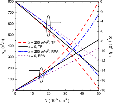
Figure 1: (Color online) The longitudinal conductivity and CISP scattered by screened charged impurities as a function of the surface carrier density for both TF screening and RPA screening.

It is seen that the polarizability function (III.4) satisfies $\Pi(q,\theta_{\bm{q}};\omega)=\Pi(q,\theta_{\bm{q}}-\pi;\omega)=\Pi(q,\theta_{\bm{q}}+\pi;\omega)$. Consequently, the angle relation of scattering potential (22) still holds for this screened Coulomb potential. Hence, when the carriers are scattered by the screened Coulomb form, only the longitudinal conductivity and $y$-component of CISP are nonzero. Now we numerically calculate the longitudinal conductivity and spin polarization for both TF screening and RPA screening. The following parameters in Bi₂Te₃ are used in the calculation:Fu266801 ; Dimitrie Fermi velocity $v_{\rm F}=2.55\,{\rm eV\cdot\AA}$, warping parameter $\lambda=250\,{\rm eV\cdot\AA^{3}}$, impurity density $n_{i}=10^{13}\,{\rm cm}^{-2}$, the static dielectric constant $\kappa=200$, and dc electric field $E=10\,{\rm V/m}$. The results are plotted in Fig. 1. The corresponding conductivity and CISP for $\lambda=0$ are also plotted for comparison. For vanishing $\lambda$, the conductivity and spin polarization linearly rely on the surface carrier density $N$, which agrees with the previous theoretical calculation.Dimitrie With increasing the density $N$, the hexagonal warping effect becomes important for both TF and RPA screened Coulomb potential, leading to nonlinear characters of conductivity and CISP. The magnitudes of conductivity and spin polarization in the presence of warping effect are larger than the ones in the absence of warping. Furthermore, we verify that, $\sigma_{xx}=c_{1}N+c_{2}N^{2}$, $S_{y}=c_{3}N+c_{4}N^{2}$, in contrast to the ones of short-range scattering. We note that the TF screening is the long-wavelength limit of RPA dielectric function. At the same time, for finite magnitude of momentum, the RPA screening is weaker than the TF one. Hence, the conductivity for TF screened Coulomb potential is larger than the RPA one at the same $\lambda$.

Here we have assumed that the impurities are located right on the surface. However, the charged impurities in the bulk of TIs may also contribute to the surface transport. These remote impurities will enhance the magnitude of conductivity and spin polarization. One can deduce that the warping will lead to a large increase of the magnitude of surface transport quantities even in the presence of remote impurities.

Note that the classical surface conductivity of Bi₂Se₃ was observed by using a gate electrode.Kim It showed a linear carrier density dependence when the density is smaller than the carrier density above which the bulk conduction band is populated. In Bi₂Se₃, the hexagonal warping is small enough to be omitted completely. Hence, this experiment verified the previous theoretical prediction well.Dimitrie However, for the surface states of TI where the warping term cannot be neglected, such as Bi₂Te₃, the linear dependence will be broken and a quadratic relation also appears. Therefore, our prediction suggests that the surface transport in Bi₂Te₃ should be different from the one of Bi₂Se₃ and it should be very careful when one analyzes the surface transport data of Bi₂Te₃.

IV classical transport in the presence of magnetic scattering

Let us now address the magnetic scattering case in the classical diffusion regime, where the scattering potential readsLiu156603

$$\widetilde{V}(\bm{r})= \sum_{\{\bm{R}_{\alpha}\}}\{J_{\parallel}[s_{x}(\bm{r})\tilde{S}_{x}(\bm{R}_{\alpha})+s_{y}(\bm{r})\tilde{S}_{y}(\bm{R}_{\alpha})]$$

$$+J_{z}s_{z}(\bm{r})\tilde{S}_{z}(\bm{R}_{\alpha})\}\delta(\bm{r}-\bm{R}_{\alpha}).$$ (37)

Here $\bm{s}=\frac{1}{2}\bm{\sigma}$ is the spin vector of electron, and ${\tilde{\bm{S}}}$ is the impurity spin, and $J_{\parallel}$, $J_{z}$ are the coupling parameters.

For simplicity, we assume the classical magnetic impurities and their spins polarized in the $z$ direction. This kind of potential conserves the $z$-component of the carrier spin. It is known that magnetic doping will open a gap in the helical Dirac cone.chensci From the mean field approximation, the gap has the form:culcer2010anomalous $\Delta=2n_{i}J_{z}\tilde{S}$. Hence, for high mobility sample, the density of magnetic impurities is small enough, and then the gap opened by the magnetic doping is considered to be very small. When $\Delta\ll\varepsilon_{\rm F}$, the effect of gap on the energy spectrum, group velocity, etc. could be neglected safely. Therefore, we can only consider the scattering effect of magnetic impurities. Applying the similar procedure as the nonmagnetic scattering situation, the analogous kinetic equations can be derived only by replacing $V(\bm{k}-\bm{q})$, $a_{1}(\bm{k},\bm{q})$, $a_{2}(\bm{k},\bm{q})$, and $a_{3}(\bm{k},\bm{q})$ in Eqs. (9)-(11) with $u_{\rm M}$, $a_{1}^{\rm M}(\bm{k},\bm{q})$, $a_{2}^{\rm M}(\bm{k},\bm{q})$, and $a_{3}^{\rm M}(\bm{k},\bm{q})$. Here $u_{\rm M}=J_{z}\tilde{S}/2$ and

$$a_{1}^{\rm M}(\bm{k},\bm{q})= -\frac{1}{2}\big{[}\sin 2\beta_{\bm{k}}\sin 2\beta_{\bm{q}}\cos(\theta_{\bm{k}}-\theta_{\bm{q}})$$

$$-\cos 2\beta_{\bm{k}}\cos 2\beta_{\bm{q}}-1\big{]},$$ (38)

$$a_{2}^{\rm M}(\bm{k},\bm{q})= -\frac{1}{2}\big{[}\cos 2\beta_{\bm{k}}\sin 2\beta_{\bm{q}}\cos(\theta_{\bm{k}}-\theta_{\bm{q}})$$

$$+\sin 2\beta_{\bm{k}}\cos 2\beta_{\bm{q}}\big{]},$$ (39)

$$a_{3}^{\rm M}(\bm{k},\bm{q})= \frac{1}{2}\sin 2\beta_{\bm{q}}\sin(\theta_{\bm{k}}-\theta_{\bm{q}}).$$ (40)

Taking into account the symmetrical property of distribution function, it is also verified that only the longitudinal conductivity and $y$-component of CISP are nonzero for this magnetic scattering. Eventually, the expressions of them are given by Eqs. (23) and (24).

We first assume that the warping parameter is weak. Thus the kinetic equation can be solved analytically and the diagonal element of the impurity-related distribution is

$$\rho_{22}^{(2)}(\bm{k})= -\frac{2eE}{3n_{i}u_{\rm M}^{2}}\Bigg{[}\frac{2v_{\rm F}^{3}}{\varepsilon_{\rm F}}\cos\theta_{\bm{k}}+\lambda^{2}\frac{\varepsilon_{\rm F}^{3}}{2v_{\rm F}^{3}}\bigg{(}\frac{35}{3}\cos\theta_{\bm{k}}$$

$$+\frac{17}{2}\cos 5\theta_{\bm{k}}-\frac{1}{2}\cos 7\theta_{\bm{k}}\bigg{)}\Bigg{]}\delta(\varepsilon_{\bm{k}2}-\varepsilon_{\rm F}).$$ (41)

Hence, the charge conductivity and CISP are written as

$$\sigma_{xx}= \frac{e^{2}}{9\pi n_{i}u^{2}_{\rm M}}\left[3v_{\rm F}^{2}+8\left(\frac{\varepsilon_{\rm F}}{v_{\rm F}}\right)^{4}\lambda^{2}\right],$$

$$= \frac{e^{2}}{9\pi n_{i}u^{2}_{\rm M}}\left(3v_{\rm F}^{2}+128\pi^{2}\lambda^{2}N^{2}\right),$$ (42)

$$S_{y}= -\frac{eE}{36\pi n_{i}u^{2}_{\rm M}}\left(6v_{\rm F}+7\frac{\varepsilon_{\rm F}^{4}}{v_{\rm F}^{5}}\lambda^{2}\right),$$

$$= -\frac{eE}{18\pi v_{\rm F}n_{i}u_{\rm M}^{2}}\left(3v_{\rm F}^{2}+56\pi^{2}\lambda^{2}N^{2}\right).$$ (43)

Compared with the short-range nonmagnetic scattering, similar density-dependent behaviors have also been seen for this magnetic one. However, the concrete coefficients are distinct, completely.

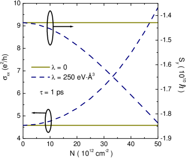
Figure 2: (Color online) The longitudinal conductivity and $y$-component of CISP scattered by magnetic impurities as a function of the surface carrier density. The other parameters are the same as the ones in Sec. III.4.2.

To go beyond the weak warping case, we now numerically solve the kinetic equations. Setting the relaxation time $\tau={2v_{\rm F}}/({n_{i}u_{\rm M}^{2}\sqrt{4\pi N_{0}}})=1\,{\rm ps}$ with $N_{0}=10^{12}\,{\rm cm}^{-2}$, the obtained longitudinal conductivity and spin polarization are plotted in Fig. 2. For comparison, the conductivity and CISP without warping effect are also calculated. It is seen that for fixed relaxation time the warping term also has important role on the surface transport of a three-dimensional TI. The magnitude of longitudinal conductivity and spin polarization increase drastically with increasing the surface density. Note that the above analytical results Eqs. (42) and (43) are valid for weak warping. That is a density $N\ll v_{\rm F}/(5\pi\lambda)\approx 5\times 10^{12}\,{\rm cm}^{-2}$. For example, if we use the approximation result (42) to estimate the conductivity, the resultant $\sigma_{xx}\approx 171.3\,{\rm e^{2}/h}$ when $N=30\times 10^{12}\,{\rm cm}^{-2}$. This value is much larger than the numerical one. At the same time, it can be confirmed from the numerical calculation that the additional terms $\varpropto N$ also contribute to conductivity and spin polarization for nonvanishing warping.

V quantum correction

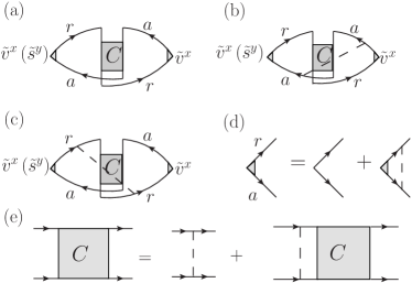
Figure 3: The diagrams for the quantum corrections to surface conductivity and spin polarization of TI. (a) Bare and [(b)-(c)] two dressed Hikami boxes. (d) Equation for the vertex correction to velocity and average spin in the ladder approximation. (e) Bethe-Salpeter equation for the Cooperon. The arrowed solid and dashed lines represent the retarded and advanced Green’s functions, and scattering potential, respectively.

We now focus on the effect of weak warping on the quantum corrections to conductivity and spin polarization. For this surface state, the Berry phase is calculated as

$$\gamma= -i\int_{0}^{2\pi}d\theta_{\bm{k}}\langle\varphi_{\bm{k}2}|\frac{\partial}{\partial\theta_{\bm{k}}}|\varphi_{\bm{k}2}\rangle$$

$$= \frac{1}{2}\int_{0}^{2\pi}d\theta_{\bm{k}}\left[1+\frac{\lambda k_{\rm F}^{3}(\theta_{\bm{k}})}{\varepsilon_{\rm F}}\cos 3\theta_{\bm{k}}\right].$$ (44)

In connection with Eq. (33), the Berry phase equals $\pi$. Hence, the weak anti-localization is expected for the surface state even in the presence of warping effect.

Using equilibrium Green’s function, the quantum corrections are described by the diagrams in Fig. 3. Firstly, we consider the short-range nonmagnetic scattering. Note that in the previous work the authors replaced the energy spectrum by its angle average one to investigate the quantum correction. In our situation the angle dependence of warping is taken into account, hence, our treatment is beyond this approximation. We also assume that the Fermi energy is in the gap of bulk band, and crosses the upper band of surface state. Under Born approximation, the impurity-averaged equilibrium retarded and advanced Green’s functions are given by

$${\hat{G}}^{r/a}_{\bm{k}}(\epsilon)=\frac{1}{\epsilon-\epsilon_{\bm{k}}\pm i/2\tau_{e}},$$ (45)

with the relaxation time $\tfrac{1}{\tau_{e}}=n_{i}u^{2}\tfrac{\varepsilon_{\rm F}}{4v_{\rm F}^{8}}(2v_{\rm F}^{6}-3\varepsilon_{\rm F}^{4}\lambda^{2})$. We add a hat on the equilibrium Green’s functions to distinguish them from the nonequilibrium Green’s functions. Notice that we have used a matrix distribution function to discuss the classical transport. However, in the absence of interband transition process and for usual elastic scattering, the matrix distribution reduces to a scalar one [see Eqs. (9), (23) and (24)]. Hence, the kinetic equation approach is in principle equivalent to the one-band equilibrium Green’s functions approach. The kinetic equation approach can easily deal with momentum-dependent scattering in classical transport, but it is difficult to discuss the quantum correction. Therefore, we treat the weak anti-localization in the diagrammatic approach by using equilibrium Green’s functions. Below, the word “equilibrium” will be omitted for brevity.

In the calculation, the vertex corrections to the bare velocity and average spin Fig. 3 (d) should be taken into account, which are written as

$$\tilde{v}^{x}_{\bm{k}} =2v_{\rm F}\cos\theta_{\bm{k}}+\frac{\lambda^{2}k^{4}}{2v_{\rm F}}\left(3\cos\theta_{\bm{k}}+\frac{5}{2}\cos 5\theta_{\bm{k}}-\frac{1}{2}\cos 7\theta_{\bm{k}}\right),$$ (46)

$$\tilde{s}^{y}_{\bm{k}} =\cos\theta_{\bm{k}}-\frac{\lambda^{2}k^{4}}{4v_{\rm F}^{2}}\left(3\cos\theta_{\bm{k}}+\frac{1}{2}\cos 5\theta_{\bm{k}}+\frac{1}{2}\cos 7\theta_{\bm{k}}\right).$$ (47)

Different from the topological surface states in the absence of hexagonal warping, the velocity and spin vertex become anisotropic. This anisotropy is very important and will lead to the density dependence of quantum correction. Note that in the absence of warping the group velocity $v^{x}_{\bm{k}}={\partial\epsilon_{\bm{k}}}/{\partial k_{x}}|_{\lambda=0}=v_{\rm F}\cos\theta_{\bm{k}}$ and average spin $s^{y}_{\bm{k}}=\tfrac{1}{2}\langle\varphi_{\bm{k}2}|\hat{\sigma}_{y}|\varphi_{\bm{k}2}\rangle|_{\lambda=0}=\tfrac{1}{2}\cos\theta_{\bm{k}}$. Therefore, for vanishing $\lambda$, the velocity vertex reduces toMcCann2006 $\tilde{v}^{x}_{\bm{k}}=2v^{x}_{\bm{k}}$.

In addition to the bare Hikami box Fig. 3 (a), two dresses Hikami boxes Fig. 3 (b)-(c) are also needed in the calculation of quantum corrections and the total corrections of charge conductivity is given by

$$\delta\sigma_{xx}=\delta\sigma_{xx}^{(1)}+\delta\sigma_{xx}^{(2)}+\delta\sigma_{xx}^{(3)},$$ (48)

where the quantum correction due to bare Hikami box

$$\delta\sigma_{xx}^{(1)}=\frac{e^{2}}{2\pi}\sum_{\bm{k},\bm{q}}\tilde{v}^{x}_{\bm{k}}\hat{G}_{\bm{k}}^{r}\hat{G}_{\bm{q}-\bm{k}}^{r}\tilde{v}^{x}_{\bm{q}-\bm{k}}\hat{G}_{\bm{q}-\bm{k}}^{a}\hat{G}_{\bm{k}}^{a}C(\bm{q}),$$ (49)

and the quantum corrections due to two dressed Hikami boxes

$$\delta\sigma_{xx}^{(2)}= \frac{e^{2}}{2\pi}\sum_{\bm{k},\bm{q},\bm{k}^{\prime}}\tilde{v}^{x}_{\bm{k}}\hat{G}_{\bm{k}}^{r}\hat{G}_{\bm{k}^{\prime}}^{r}\langle|\xi_{\bm{k}\bm{k}^{\prime}}|^{2}\rangle_{\rm imp}\hat{G}_{\bm{q}-\bm{k}}^{r}\hat{G}_{\bm{q}-\bm{k}^{\prime}}^{r}$$

$$\times\tilde{v}^{x}_{\bm{q}-\bm{k}^{\prime}}\hat{G}_{\bm{q}-\bm{k}^{\prime}}^{a}\hat{G}_{\bm{k}}^{a}C(\bm{q}),$$ (50)

$$\delta\sigma_{xx}^{(3)}= \frac{e^{2}}{2\pi}\sum_{\bm{k},\bm{q},\bm{k}^{\prime}}\tilde{v}^{x}_{\bm{k}}\hat{G}_{\bm{k}}^{r}\hat{G}_{\bm{q}-\bm{k}^{\prime}}^{r}\langle|\xi_{\bm{k}\bm{k}^{\prime}}|^{2}\rangle_{\rm imp}\hat{G}_{\bm{q}-\bm{k}^{\prime}}^{a}\hat{G}_{\bm{q}-\bm{k}}^{a}$$

$$\times\tilde{v}^{x}_{\bm{q}-\bm{k}^{\prime}}\hat{G}_{\bm{k}^{\prime}}^{a}\hat{G}_{\bm{k}}^{a}C(\bm{q}).$$ (51)

Here $\xi_{\bm{k}\bm{k}^{\prime}}=\int d\bm{r}e^{i(\bm{k}^{\prime}-\bm{k})\cdot\bm{r}}\langle\varphi_{\bm{k}2}|\widetilde{V}(\bm{r})|\varphi_{\bm{k}^{\prime}2}\rangle$ is the scattering amplitude between two eigenstates. $\langle\cdots\rangle_{\rm imp}$ means average over all possible configurations of random impurity. Consequently, for $\delta$-form impurity scattering, $\langle|\xi_{\bm{k}\bm{k}^{\prime}}|^{2}\rangle_{\rm imp}=n_{i}u^{2}\langle\varphi_{\bm{k}2}|\varphi_{\bm{k}^{\prime}2}\rangle\langle\varphi_{\bm{k}^{\prime}2}|\varphi_{\bm{k}2}\rangle$. Since the Cooperon $C(\bm{q})$ diverges as $q\rightarrow 0$, hence the most divergent terms could be obtained by setting $\bm{q}=0$ for velocity vertex, retarded and advanced Green’s functions in the above expressions. Performing momentum $\bm{k}$ and $\bm{k}^{\prime}$ integrals, the total conductivity correction is written as

$$\delta\sigma_{xx}=-\frac{e^{2}}{\pi}\varepsilon_{\rm F}\tau_{e}^{3}\left(1+\frac{\lambda^{2}\varepsilon_{\rm F}^{4}}{2v_{\rm F}^{6}}\right)\sum_{\bm{q}}C(\bm{q}).$$ (52)

For vanishing $\lambda$, this result is in accordance with the one in Ref. lu2011competing, . Similarly, the total spin polarization correction is given by

$$\delta S_{y}=\frac{eE}{2\pi}\frac{\varepsilon_{\rm F}\tau_{e}^{3}}{v_{\rm F}}\left(1-\frac{\lambda^{2}\varepsilon_{\rm F}^{4}}{v_{\rm F}^{6}}\right)\sum_{\bm{q}}C(\bm{q}).$$ (53)

The Cooperon satisfies the Bethe-Salpeter equation Fig. 3 (e)

$$C_{\bm{k}_{1}\bm{k}_{2}}= C_{\bm{k}_{1}\bm{k}_{2}}^{(0)}+\sum_{\bm{k}^{\prime}}C_{\bm{k}_{1}\bm{k}^{\prime}}^{(0)}G_{\bm{k}^{\prime}}^{r}G_{\bm{q}-\bm{k}^{\prime}}^{a}C_{\bm{k}^{\prime}\bm{k}_{2}}$$

$$= C_{\bm{k}_{1}\bm{k}_{2}}^{(0)}+\int\frac{dk^{\prime}d\theta_{\bm{k}^{\prime}}}{(2\pi)^{2}}F(\bm{k}_{1},\bm{k}^{\prime},\bm{q})C_{\bm{k}^{\prime}\bm{k}_{2}},$$ (54)

where $\bm{k}_{1}+\bm{k}_{2}=\bm{q}$, $F(\bm{k}_{1},\bm{k}^{\prime},\bm{q})=k^{\prime}C_{\bm{k}_{1}\bm{k}^{\prime}}^{(0)}\hat{G}_{\bm{k}^{\prime}}^{r}\hat{G}_{\bm{q}-\bm{k}^{\prime}}^{a}$, and by expanding up to $\lambda^{2}$, the bare vertex $C_{\bm{k}_{1}\bm{k}_{2}}^{(0)}$ for small $q$ is written as

$$C_{\bm{k}_{1}\bm{k}_{2}}^{(0)}=\Upsilon^{(0)}_{\bm{k}_{1}\bm{k}_{2}}+\lambda^{2}\Upsilon^{(2)}_{\bm{k}_{1}\bm{k}_{2}},$$ (55)

with

$$\Upsilon^{(0)}_{\bm{k}_{1}\bm{k}_{2}}=\frac{v_{\rm F}^{2}}{2\varepsilon_{\rm F}\tau_{e}}\left[1+2e^{i(\theta_{\bm{k}_{1}}-\theta_{\bm{k}_{2}})}+e^{2i(\theta_{\bm{k}_{1}}-\theta_{\bm{k}_{2}})}\right].$$ (56)

The expression of $\Upsilon^{(2)}_{\bm{k}_{1}\bm{k}_{2}}$ is long and we do not write it here. For weak warping, the solution of Eq. (V) is found as $C_{\bm{k}_{1}\bm{k}_{2}}=\Lambda_{\bm{k}_{1}\bm{k}_{2}}^{(0)}+\lambda^{2}\Lambda_{\bm{k}_{1}\bm{k}_{2}}^{(2)}$. $\Lambda_{\bm{k}_{1}\bm{k}_{2}}^{(0)}$ and $\Lambda_{\bm{k}_{1}\bm{k}_{2}}^{(2)}$ are independent of $\lambda$. With the help of the expansion $F(\bm{k}_{1},\bm{k}^{\prime},\bm{q})=F^{(0)}(\bm{k}_{1},\bm{k}^{\prime},\bm{q})+\lambda^{2}F^{(2)}(\bm{k}_{1},\bm{k}^{\prime},\bm{q})$, $\Lambda_{\bm{k}_{1}\bm{k}_{2}}^{(0)}$ and $\Lambda_{\bm{k}_{1}\bm{k}_{2}}^{(2)}$ are determined by the following equations:

$$\Lambda_{\bm{k}_{1}\bm{k}_{2}}^{(0)}= \Upsilon^{(0)}_{\bm{k}_{1}\bm{k}_{2}}+\int\frac{dk^{\prime}d\theta_{\bm{k}^{\prime}}}{(2\pi)^{2}}F^{(0)}(\bm{k}_{1},\bm{k}^{\prime},\bm{q})\Lambda_{\bm{k}_{1}\bm{k}_{2}}^{(0)},$$ (57)

$$\Lambda_{\bm{k}_{1}\bm{k}_{2}}^{(2)}= \Upsilon^{(2)}_{\bm{k}_{1}\bm{k}_{2}}+\int\frac{dk^{\prime}d\theta_{\bm{k}^{\prime}}}{(2\pi)^{2}}F^{(2)}(\bm{k}_{1},\bm{k}^{\prime},\bm{q})\Lambda_{\bm{k}^{\prime}\bm{k}_{2}}^{(0)}$$

$$+\int\frac{dk^{\prime}d\theta_{\bm{k}^{\prime}}}{(2\pi)^{2}}F^{(0)}(\bm{k}_{1},\bm{k}^{\prime},\bm{q})\Lambda_{\bm{k}^{\prime}\bm{k}_{2}}^{(2)}.$$ (58)

$\Lambda_{\bm{k}_{1}\bm{k}_{2}}^{(0)}$ can be acquired from Eq. (57) and then we can obtain $\Lambda_{\bm{k}_{1}\bm{k}_{2}}^{(2)}$ From Eq. (58). It is found that $F^{(0)}(\bm{k}_{1},\bm{k}^{\prime},\bm{q})$ relies on $\theta_{\bm{k}_{1}}$ through $\cos\theta_{\bm{k}_{1}}$, $\sin\theta_{\bm{k}_{1}}$, $\cos 2\theta_{\bm{k}_{1}}$, and $\sin 2\theta_{\bm{k}_{1}}$. Hence, $\Lambda_{\bm{k}_{1}\bm{k}_{2}}^{(0)}$ and $\Lambda_{\bm{k}_{1}\bm{k}_{2}}^{(2)}$ have the forms:

$$\Lambda_{\bm{k}_{1}\bm{k}_{2}}^{(0)}= \Upsilon^{(0)}_{\bm{k}_{1}\bm{k}_{2}}+\mathcal{A}_{0}+\mathcal{A}_{1}\cos\theta_{\bm{k}_{1}}+\mathcal{B}_{1}\sin\theta_{\bm{k}_{1}}$$

$$+\mathcal{A}_{2}\cos 2\theta_{\bm{k}_{1}}+\mathcal{B}_{2}\sin 2\theta_{\bm{k}_{1}},$$ (59)

$$\Lambda_{\bm{k}_{1}\bm{k}_{2}}^{(2)}= \Upsilon^{(2)}_{\bm{k}_{1}\bm{k}_{2}}+\int\frac{dk^{\prime}d\theta_{\bm{k}^{\prime}}}{(2\pi)^{2}}F^{(2)}(\bm{k}_{1},\bm{k}^{\prime},\bm{q})\Lambda_{\bm{k}^{\prime}\bm{k}_{2}}^{(0)}$$

$$+\mathcal{C}_{0}+\mathcal{C}_{1}\cos\theta_{\bm{k}_{1}}+\mathcal{D}_{1}\sin\theta_{\bm{k}_{1}}$$

$$+\mathcal{C}_{2}\cos 2\theta_{\bm{k}_{1}}+\mathcal{D}_{2}\sin 2\theta_{\bm{k}_{1}}.$$ (60)

The above coefficients $\mathcal{A}_{i}$, $\mathcal{B}_{j}$, $\mathcal{C}_{i}$, and $\mathcal{D}_{j}$ ($i=0,1,2$, $j=1,2$) are independent of $\theta_{\bm{k}_{1}}$ and can be determined by Eqs. (57) and (58). The derivation is tedious but direct. By setting $\bm{k}_{1}=\bm{k}$, $\bm{k}_{2}=\bm{q}-\bm{k}$ and $\theta_{\bm{k}_{1}}-\theta_{\bm{k}_{2}}=\pi$ for small $q$ and collecting the most divergent terms, finally, the Cooperon is obtained as

$$C(\bm{q})=-\frac{1}{\varepsilon_{\rm F}\tau_{e}^{3}q^{2}}-\frac{5}{4}\frac{\lambda^{2}\varepsilon_{\rm F}^{3}}{v_{\rm F}^{6}\tau_{e}^{3}q^{2}}.$$ (61)

By performing the integration over $q$ between $1/l_{\phi}$ and $1/l$, the logarithmic correction to the conductivity and spin polarization are found as

$$\delta\sigma_{xx}= \frac{e^{2}}{4\pi^{2}}\left(1+\frac{3}{4}\frac{\lambda^{2}\varepsilon_{\rm F}^{4}}{v_{\rm F}^{6}}\right)\ln\frac{\tau_{\phi}}{\tau_{e}},$$ (62)

$$\delta S_{y}= -\frac{eE}{8\pi^{2}v_{\rm F}}\left(1+\frac{1}{4}\frac{\lambda^{2}\varepsilon_{\rm F}^{4}}{v_{\rm F}^{6}}\right)\ln\frac{\tau_{\phi}}{\tau_{e}}.$$ (63)

Here we have used the relations $l=\sqrt{D\tau_{e}}$ and $l_{\phi}=\sqrt{D\tau_{\phi}}$ with $D$ the diffusion constant. It is useful to rewrite the conductivity correction as $\delta\sigma_{xx}=-\alpha\tfrac{e^{2}}{2\pi^{2}}\ln\frac{\tau_{\phi}}{\tau_{e}}$. Therefore, the $\alpha$ has the form:

$$\alpha= -\frac{1}{2}\left(1+\frac{3}{4}\frac{\lambda^{2}\varepsilon_{\rm F}^{4}}{v_{\rm F}^{6}}\right),$$

$$= -\frac{1}{2}\left(1+\frac{12\pi^{2}\lambda^{2}}{v_{\rm F}^{2}}N^{2}\right).$$ (64)

The hexagonal warping makes the prefactor $\alpha$ quadratically depend on the carrier density and is always smaller than $-\tfrac{1}{2}$, in vivid contrast with the angle-average approximation.tkachov2011weak For vanishing warping, this factor becomes $-\tfrac{1}{2}$, in agreement with the theoretical work.lu2011competing We note that the above formula is fulfilled for weak warping. On the other hand, one can estimate the $\alpha$ for Bi₂Te₃ at low surface density $N\ll 10^{13}\,{\rm cm}^{-2}$. For instance, $\alpha\approx-0.506$ when $N=10^{12}\,{\rm cm}^{-2}$. However, the value of the $\alpha$ obtained from fit in recent experimentHongTao2011 is $-0.39$, which is larger than $-0.5$, conflicting with our formula. This may be due to the inevitable bulk states contribution in three-dimensional TIs.lu2011weak The experimental observation of $\alpha$ is a collective result of the surface bands and bulk bands. The bulk channels may result in a weak localization term, which could reduce or even compensate the weak anti-localization arising from the surface states. Therefore, a larger value of $\alpha$ is obtained experimentally. In contrast to the surface bands, the bulk subbands of TIs have a quadratic term and large band gaps. As a result, a different density-dependent behavior of quantum correction is expected for the bulk channels. A quantitative measurement of the carrier-density-dependent surface conductivity correction could be helpful for distinguishing the surface contribution from the bulk one.

In the presence of magnetic scattering, the divergence of $C(\bm{q})$ when $q\rightarrow 0$ vanishes, which is analogous to the case without warping.lu2011competing Therefore the logarithmic correction disappears, and it could be deduced that the magnetic scattering suppresses the weak anti-localization effect in the presence of both magnetic and nonmagnetic scattering. This is in accordance with experimental observation.HongTao2011

VI conclusion

In summary, we have investigated the surface transport of a three-dimensional TI both in classical and quantum diffusive regimes. In this study, we include the role of the hexagonal warping correction of Fermi surface. It is found that the hexagonal warping has drastic effects on the surface conductivity and CISP of a three-dimensional TI for both nonmagnetic and magnetic elastic scattering. For surface state with large warping, such as Bi₂Te₃, an additional quadratic carrier density dependence is found in both two regimes. Because the carrier density could be controlled by the gate voltage, hence, we hope that our predictions will soon be verified experimentally.

References

• (1) C. L. Kane and E. J. Mele, Phys. Rev. Lett. 95, 226801 (2005).
• (2) X.-L. Qi, T. L. Hughes, and S.-C. Zhang, Phys. Rev. B 78, 195424 (2008).
• (3) X. L. Qi and S. C. Zhang, arXiv:1008.2026 (unpublished).
• (4) L. Fu and C. L. Kane, Phys. Rev. Lett. 100, 096407 (2008).
• (5) I. Garate and M. Franz, Phys. Rev. Lett. 104, 146802 (2010).
• (6) C. Wu, B. A. Bernevig, and S.-C. Zhang, Phys. Rev. Lett. 96, 106401 (2006).
• (7) C. Xu, J. E. Moore, Phys. Rev. B 73, 045322 (2006).
• (8) K. S. Novoselov, A. K. Geim, S. V. Morozov, D. Jiang, M. I. Katsnelson, I. V. Grigorieva, S. V. Dubonos, and A. A. Firsov, Nature 438, 197 (2005).
• (9) D. Hsieh, D. Qian, L. Wray, Y. Xia, Y. S. Hor, R. J. Cava, and M. Z. Hasan, Nature 452, 970 (2008).
• (10) D. Hsieh, Y. Xia, L. Wray, D. Qian, A. Pal, J. H. Dil, J. Osterwalder, F. Meier, G. Bihlmayer, C. L. Kane, Y. S. Hor, R. J. Cava, and M. Z. Hasan, Science 323, 919 (2009).
• (11) Y. L. Chen, J. G. Analytis, J.-H. Chu, Z. K. Liu, S.-K. Mo, X. L. Qi, H. J. Zhang, D. H. Lu, X. Dai, Z. Fang, S. C. Zhang, I. R. Fisher, Z. Hussain, and Z.-X. Shen, Science 325, 178 (2009).
• (12) J. G. Checkelsky, Y. S. Hor, R. J. Cava, and N. P. Ong, Phys. Rev. Lett. 106, 196801 (2011).
• (13) D. Culcer, E. H. Hwang, T. D. Stanescu, and S. Das Sarma, Phys. Rev. B 82, 155457 (2010).
• (14) D. Kim, S. Cho, N. P. Butch, P. Syers, K. Kirshenbaum, J. Paglione, and M. S. Fuhrer, arXiv:1105.1410 (unpublished).
• (15) D. Culcer and S. Das Sarma, Phys. Rev. B 83, 245441 (2011).
• (16) S. Giraud and R. Egger, Phys. Rev. B 83, 245322 (2011).
• (17) T. Yokoyama and S. Murakami, Phys. Rev. B 83, 161407(R) (2011).
• (18) J. Chen, H. J. Qin, F. Yang, J. Liu, T. Guan, F. M. Qu, G. H. Zhang, J. R. Shi, X. C. Xie, C. L. Yang, K. H. Wu, Y. Q. Li, and L. Lu, Phys. Rev. Lett. 105, 176602 (2010).
• (19) H.-T. He, G. Wang, T. Zhang, I.-K. Sou, G. K. L. Wong, J.-N. Wang, H.-Z. Lu, S.-Q. Shen, and F.-C. Zhang, Phys. Rev. Lett. 106, 166805 (2011).
• (20) M. Liu, C.-Z. Chang, Z. Zhang, Y. Zhang, W. Ruan, K. He, L.-l. Wang, X. Chen, J.-F. Jia, S.-C. Zhang, Q.-K. Xue, X. Ma, and Y. Wang, Phys. Rev. B 83, 165440 (2011).
• (21) H. Z. Lu, J. Shi, and S. Q. Shen, Phys. Rev. Lett. 107, 076801 (2011).
• (22) G. Tkachov and E. M. Hankiewicz, Phys. Rev. B 84, 035444 (2011).
• (23) E. McCann, K. Kechedzhi, V. I. Fal’ko, H. Suzuura, T. Ando, and B. L. Altshuler, Phys. Rev. Lett. 97, 146805 (2006).
• (24) Z. Alpichshev, J. G. Analytis, J.-H. Chu, I. R. Fisher, Y. L. Chen, Z. X. Shen, A. Fang, and A. Kapitulnik, Phys. Rev. Lett. 104, 016401 (2010).
• (25) L. Fu, Phys. Rev. Lett. 103, 266801 (2009).
• (26) H. Haug and A.-P. Jauho, Quantum Kinetics in Transport and Optics of Semiconductors (Springer, 1996).
• (27) M. I. D’yakonov and V. I. Perel’, Phys. Lett. A 35, 459 (1971).
• (28) V. M. Edelstein, Solid State Commun. 73, 233 (1990).
• (29) C. M. Wang, S. Y. Liu, Q. Lin, X. L. Lei, and M. Q. Pang, J. Phys.: Condens. Matter 22, 095803 (2010).
• (30) C. M. Wang, M. Q. Pang, S. Y. Liu, and X. L. Lei, Phys. Lett. A 374, 1286 (2010).
• (31) Y. Tokura, Phys. Rev. B 58, 7151 (1998).
• (32) Y. K. Kato, R. C. Myers, A. C. Gossard, and D. D. Awschalom, Science 306, 1910 (2004).
• (33) F. Stern, Phys. Rev. Lett. 18, 546 (1967).
• (34) B. Wunsch, T. Stauber, F. Sols, and F. Guinea, New J. Phys. 8, 318 (2006).
• (35) E. H. Hwang and S. Das Sarma, Phys. Rev. B 75, 205418 (2007).
• (36) Q. Liu, C.-X. Liu, C. Xu, X.-L. Qi, and S.-C. Zhang, Phys. Rev. Lett. 102, 156603 (2009).
• (37) Y. L. Chen, J.-H. Chu, J. G. Analytis, Z. K. Liu, K. Igarashi, H.-H. Kuo, X. L. Qi, S. K. Mo, R. G. Moore, D. H. Lu, M. Hashimoto, T. Sasagawa, S. C. Zhang, I. R. Fisher, Z. Hussain, and Z. X. Shen, Science 329, 659 (2010).
• (38) H. Z. Lu and S.-Q. Shen, Phys. Rev. B 84, 125138 (2011).