Universal Finite Temperature Properties of a Three Dimensional Quantum Antiferromagnet in the Vicinity of a Quantum Critical Point

Abstract

We consider a 3-dimensional quantum antiferromagnet which can be driven through a quantum critical point (QCP) by varying a tuning parameter g. Starting from the magnetically ordered phase, the Néel temperature will decrease to zero as the QCP is approached. From a generic quantum field theory, together with numerical results from a specific microscopic Heisenberg spin model, we demonstrate the existence of universal behaviour near the QCP. We compare our results with available data for $TlCuCl_{3}$.

The subject of continuous Quantum Phase Transitions (QPT’s) and the behaviour of quantum systems in the vicinity of the corresponding quantum critical points is a frontier area of research both in theory and in experiment. Sachdevphystoday ; sachdev2010 A QPT is a transition at zero temperature, in the nature of the ground state, and is due to quantum fluctuations that can be enhanced or suppressed by varying some coupling constant. In real materials QPT’s can be driven by pressure, by applied magnetic field, or by some other parameter.

In the present work we consider an O(3) QPT which occurs between a magnetically ordered Néel phase and a magnetically disordered ’valence-bond-solid’ (VBS) phase in a class of SU(2) invariant Heisenberg spin systems. This problem has attracted a great deal of attention in recent years, mainly in two-dimensional (2D) systems. It has been established that the interplay between quantum fluctuations and thermal fluctuations at low but finite temperatures influences the dynamics in the vicinity of a QPT in a highly nontrivial way Chak ; Chub . However, in 2D systems there is no finite temperature magnetic order, due to the well known Mermin-Wagner theorem. One would expect that in 3D systems (3D + time) the presence of a finite Néel temperature and an extended region of magnetic order will affect the interplay between quantum and thermal fluctuations, and lead to new features not seen in 2D. An obvious question is the nature of the vanishing of the Néel temperature and its scaling with the magnetization and with the coupling constant as the QPT is approached. To the best of our knowledge the generic problem of the finite temperature behaviour of 3D systems in the vicinity of an O(3) QPT has not been previously considered. The present work addresses this question.

Specifically, we discuss three aspects of this question. The first is to consider a general Landau-Ginzburg field theory, which is independent of the details of any microscopic model, and hence generic. The predictions of this approach are then compared with experimental results for the material TlCuCl₃. Finally we present results obtained for a specific microscopic Heisenberg spin model, obtained using a variety of series-expansion methods. While the numerical precision close to the QPT is only moderate, the results are consistent with the field theory predictions, and reinforce our conclusion that the behaviour is universal.

To develop a quantum field theoretic description we start from the standard effective Lagrangian describing an O(3) QPT, of the form zinn ; sachdev2010 ; Kulik .

$${\cal L}=\frac{1}{2}\left({\dot{\vec{\varphi}}}-[{\vec{\varphi}}\times{\vec{B}}]\right)^{2}-\frac{c^{2}}{2}\left({\bf\nabla}{\vec{\varphi}}\right)^{2}-\frac{m^{2}}{2}{\vec{\varphi}}^{2}-\frac{\alpha}{4}[{\vec{\varphi}}^{2}]^{2}$$ (1)

In the present work we consider zero magnetic field, $B=0$. The vector field ${\vec{\varphi}}$ describes the staggered magnetization. The QPT results from the mass term, assumed to be of the form $m^{2}=\lambda^{2}(g-g_{c})$, where $\lambda^{2}>0$ is a coefficient and $g$ is a coupling parameter (In TlCuCl₃ the coupling parameter is an external hydrostatic pressure). When $g>g_{c}$ the mass squared is positive and this corresponds to the magnetically disordered phase with gapped triply degenerate excitations. These are sometimes called ’triplons’ but we will use the term ’magnon’ in both phases. The zero temperature gap is

$$\Delta=m=\lambda\sqrt{g-g_{c}}\ .$$ (2)

When $g<g_{c}$ the mass squared is negative and this results in a nonzero expectation value

$$|\langle{\vec{\varphi}}\rangle|=\sqrt{\frac{|m^{2}|}{\alpha}}=\frac{\lambda}{\sqrt{\alpha}}\sqrt{g_{c}-g}\ .$$ (3)

that describes the spontaneous staggered magnetization at zero temperature. This is a magnetically ordered phase with a gapped longitudinal mode and two transverse gapless Goldstone modes. We note that $\varphi$ has dimensions of $energy^{-1/2}$, and therefore cannot be directly compared with the dimensionless staggered magnetization. The zero temperature energy of the magnetically ordered ground state is

$$E=-\frac{\lambda^{4}}{4\alpha}(g-g_{c})^{2}\ .$$ (4)

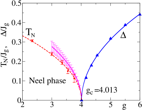
Figure 1: The phase diagram in the vicinity of a QPT. The blue triangles connected by the blue solid line show results of series expansion calculations of the spin wave gap in the magnetically disordered VBS phase. The Néel temperature is shown at $g<g_{c}$ where the system is magnetically ordered at $T<T_{N}$. The red squares connected by the red dashed line show results of series expansion calculations of $T_{N}$. The magenta solid line shows the field theory prediction for $T_{N}$.

The generic phase diagram is shown in Fig. 1. The specific parameter values shown in the figure correspond to the particular model which we consider below.

The magnetic ordering at $g<g_{c}$ is destroyed at $T>T_{N}$. To find $T_{N}$ we calculate the selfenergy $\Sigma$ shown in Fig. 2.

Figure 2: Magnon selfenergy

The four-leg vertex in Fig. 2 is due to the quartic $\alpha$-term in (1). To calculate the single loop selfenergy in the magnetically disordered phase it is sufficient to decouple the quartic interaction, $\alpha[{\vec{\varphi}}^{2}]^{2}\to\alpha\langle{\vec{\varphi}}^{2}\rangle{\vec{\varphi}}^{2}\to\Sigma{\vec{\varphi}}^{2}$. When performing the decoupling, one has to be careful about the combinatorial factor that is due to various ways of the field couplings. A straightforward calculation gives the following selfenergy in the magnetically disordered phase ($g>g_{c}$ or $T>T_{N}$ at $g<g_{c}$),

$$\Sigma=5\alpha\langle\varphi_{i}^{2}\rangle=5\alpha\sum_{\bf k}\frac{1}{\omega_{\bf k}}\left(n_{{\bf k}i}+\frac{1}{2}\right)\ ,$$ (5)

where $i$ is any of three Cartesian components of ${\vec{\varphi}}$, and $n_{{\bf k}i}=\langle a_{{\bf k}i}^{{\dagger}}a_{{\bf k}i}\rangle=1/(e^{\omega_{\bf k}/T}-1)$ is the thermal population of this component. The quantum fluctuation part of (5) is ultraviolet divergent.

$$5\alpha\sum_{\bf k}\frac{1}{2\omega_{k}} = \frac{5\alpha}{4\pi^{2}}\int_{0}^{\Lambda}\frac{k^{2}dk}{\sqrt{\delta^{2}+c^{2}k^{2}}}$$

$$\approx \frac{5\alpha}{8\pi^{2}c^{3}}\left[c^{2}\Lambda^{2}-\delta^{2}\ln\left(\frac{c\Lambda}{\delta}\right)\right]\ .$$

Here $\Lambda$ is an ultraviolet cutoff and $\delta$ is the gap in the spectrum, for example at $T=0$ and $g>g_{c}$, $\delta=\Delta$. The quadratically divergent part $\propto\Lambda^{2}$ of the self energy has to be removed by renormalization. In other words, this part is absorbed in the value of the critical coupling constant $g_{c}$. The logarithmic part depends on both the ultraviolet cutoff $\Lambda$ and the infrared cutoff $\delta$, and is therefore a real physical correction. However, we expect this logarithmic correction to be small and therefore we disregard it, (see also the discussion in Ref. Kulik ). The parameter that suppresses the correction is the prefactor $1/\pi^{2}$, and in essence it is related to the 3D character of the problem. Neither the existing experimental data presented below nor results of numerical simulations also presented below have a sufficient accuracy to pin the logarithmic corrections down. All in all this implies that the entire quantum part of the self energy is renormalized out,

$$\Sigma_{R}\approx 5\alpha\sum_{\bf k}\frac{n_{{\bf k}i}}{\omega_{\bf k}}\ ,$$ (6)

where the subscript ’R’ stands for ’renormalized’. At $T=T_{N}$ the excitation spectrum is gapless, $\delta=0$, $\omega_{\bf k}=ck$. Hence a calculation of the integral in (6) gives $\Sigma_{R}=\frac{5\alpha T_{N}^{2}}{12c^{3}}$. If the magnon spectrum is anisotropic with three different principal velocities then $c^{3}$ has to be replaced by $c_{1}c_{2}c_{3}$. The magnon gap at the Néel temperature is zero, $\delta^{2}=m^{2}+\Sigma_{R}=0$, and hence

$$T_{N}=\sqrt{\frac{12\lambda^{2}c_{1}c_{2}c_{3}}{5\alpha}}\sqrt{g_{c}-g}\ .$$ (7)

Thus, the Néel temperature is directly proportional to the zero temperature staggered magnetization (3). A similar scaling was obtained recently in Monte Carlo simulations with various kinds of models And .

Equation (7) can be compared with experimental data Ruegg for TlCuCl₃.

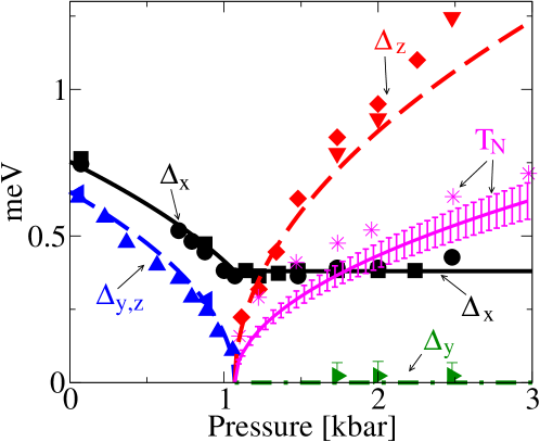
Figure 3: Zero temperature magnon gaps and Néel temperature in TlCuCl₃ versus pressure. All values are given in meV. The system is magnetically disordered at $p\leq p_{c}=1.07$kbar, and magnetically ordered at $p\geq p_{c}$. Symbols show experimental data from Ref. Ruegg and curves show theoretical results.

Values of gaps at zero temperature versus pressure are plotted in Fig. 3. The critical pressure is $p_{c}=1.07$kbar. Note that Fig. 3 is ’mirror reflected’ compared to Fig. 1, the magnetically ordered phase is at $p>p_{c}$, therefore, to compare with Eqs.(2),(3),(7) we choose $g=-p$. In the ideal situation corresponding to the action (1) one should expect triply degenerate gapped excitations in the magnetically disordered phase at $p<p_{c}$, as well as one longitudinal gapped mode ($\Delta_{z}$) and two gapless transverse modes in the magnetically ordered phase at $p>p_{c}$. In the real compound there is a small easy plane anisotropy and due to the anisotropy one of the transverse magnons in the magnetically ordered phase is gapped, with $\Delta_{x}=0.38$meV. For the same reason the triple degeneracy at $p<p_{c}$ is lifted. Disregarding the small anisotropy effects and using Eq.(2) we fit the gap in the magnetically disordered phase. The fit is shown in Fig. 3 by the blue dashed line, and results in the following value of $\lambda$, $\lambda\approx 0.66\text{ meV/kbar}^{1/2}$. Other parameters of the effective action (1) were determined in the analysis of magnon spectra and Bose condensation of magnons performed in Ref. Kulik , $c_{1}=7.09$meV, $c_{2}=1.12$meV, $c_{3}=0.51$meV, $\alpha=21(1\pm 0.2)\text{ meV}^{3}$. Substitution to Eq.(7) gives the theoretical prediction of the Néel temperature plotted in Fig. 3 by the solid magenta curve with error bars that are mainly due to uncertainty in the value of $\alpha$. This curve is very close to the experimental points, shown by magenta stars. The experimental values of the Néel temperature are slightly higher compared to the theory, especially close to the QPT point. As one would expect the magnetic anisotropy, pointed out above, leads to an enhancement of the Néel temperature. We believe this fully accounts for the discrepancy.

While the above theory is generic, and independent of the details of any microscopic model, it is interesting and important to consider a specific model and compare results with general theory. A specific microscopic model can be analysed only numerically, so below we consider a sort of numerical experiment versus the real experiment discussed above. Many previous numerical studies of QPT’s have been reported. These have been largely based on Heisenberg spin models in which the system can be tuned through a QPT by varying a particular coupling parameter in the Hamiltonian. Most of these models have been two-dimensional. Examples include antiferromagnets with strong and weak bonds, with or without frustration singh1988 ; matsumoto2001 ; wenzel2009 , and bilayer systems zheng1997 ; wang2006 , where the QPT separates a conventional Néel antiferromagnetic phase from a spin-dimerized phase with only short range correlations and no magnetic order.

Here we consider a 3D spin-1/2 Heisenberg antiferromagnet. Our model, shown in Fig.4(a), has weak and strong bonds of strength $J$ and $gJ$ respectively. For $g=1$ we have an isotropic cubic antiferromagnet, which has reduced staggered magnetization in the ground state ($M_{0}$ = 0.42 oitmaa1994 ) and a critical temperature $T/J$ = 1.89 oitmaa2004 . On the other hand, for $g>>1$ the strong bonds form spin-singlet dimers, leading to the VBS phase. A QPT separates these phases, as shown schematically in Fig.4(b).

Figure 4: (a) The model, with thin lines denoting $J$ bonds and thick lines denoting $gJ$ bonds; (b) Schematic phase diagram of the model at $T=0$.

This model has been studied previously nohadani2005 in connection with magnetic-field induced QPT’s, and the quantum critical point was located at $g_{c}=4.013\pm 0.003$, using quantum Monte Carlo (QMC) methods. However, the important questions of the universal behaviour of the Néel temperature and the dynamics of the dimerized phase were not discussed.

Our numerical calculations are based on series expansion methods oitmaa2006 , and involve several separate parts. The various series have been analysed in the usual way, via Padé approximants. The error bars shown on some of the data points are not statistical errors but ’confidence limits’ based on consistency and spread between different high order approximants. For many data points, these error bars are smaller than the point size.

We have used a ’dimer expansion’ oitmaa2006 to obtain series for the ground-state energy and the magnon energies in the VBS phase, in powers of $1/g$, to orders 11 and 8 respectively. The latter provides a direct series for the minimum gap at ${\bf k}=(\pi,\pi,0)$. Analysis of the gap series has to allow for the expected square-root singularity at $g_{c}$, and we have used a Huse transformation to remove this singularity. The resulting gap data are shown in Fig. 1 by blue triangles. Our estimate of the critical point $g_{c}$ obtained from this data is fully consistent with, although somewhat less precise than the Monte Carlo estimate $g_{c}=4.013$. We use this value in our further analysis. The gap data can be very well fitted by the expression $0.316\sqrt{g-g_{c}}$, which is shown in Fig. 1 by the blue solid line. This provides the estimate $\lambda=0.316J_{g}$, where

$$J_{g}=J(1+g)$$

is an average exchange parameter, used hereafter to set an energy scale.

Results for the magnon energies near ${\bf k}=(\pi,\pi,0)$, fitted to the expression

$$\epsilon({\bf k})=\sqrt{\Delta^{2}+c_{1}^{2}(\pi-k_{1})^{2}+c_{2}^{2}(\pi-k_{2})^{2}+c_{3}^{2}k_{3}^{2}}$$

provide estimates of the magnon velocities near the QCP, $c_{1}=c_{2}=0.516J_{g},c_{3}=0.337J_{g}$. These values contain an uncertainty up to $\pm 5\%$.

Next, we have used ’Ising expansions’ oitmaa2006 in the Néel phase to obtain series for the ground state energy and magnetization to order 12 in an anisotropy parameter $x$. These energy series, evaluated at $x$ via Padé approximants, provide the data shown in Fig.5 by red squares. The energies in the VBS phase, discussed above, are shown as black circles. As can be seen, the two energy curves, from the Néel and VBS phases respectively, meet smoothly at the QCP, as expected for a second-order transition.

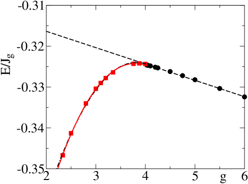
Figure 5: The ground-state energy in the Néel phase (red squares) and dimer phase (black circles) versus the coupling constant. The lines are fits to the energy, as discussed below.

This data can then be used to estimate the parameter $\alpha$ in Eq.(4). The VBS energy can be accurately fitted with a straight line $E_{VBS}/J_{g}=-0.3244-0.0040(g-g_{c})$, shown as the black dashed line in Fig. 5. The Néel data can be fitted with a quadratic expression, as in Eq.(4), $E_{N}/J_{g}=E_{VBS}(g)+0.00003-0.0101(g-g_{c})^{2}$. However this fitting is subject to uncertainty, as the energies near the QCP are only changing in the 4th figure, and the data are not that precise. Indeed, inclusion of a small cubic term in the fit changes the coefficient of the quadratic term significantly, $E_{N}/J_{g}=E_{VBS}(g)-0.00028-0.0088(g-g_{c})^{2}+0.0008(g-g_{c})^{3}$. Comparing the coefficient of the quadratic term with Eq.(4) we determine the value of the quartic coupling constant. Our final estimate is $\alpha=0.283J_{g}^{3}$, with an uncertainty of $\pm 15\%$.

Substitution of the determined parameters into Eq.(7) gives $T_{N}/J_{g}=0.275\sqrt{g_{c}-g}$. This dependence is shown in Fig. 1 by the solid magenta line with error bars. The main uncertainty, $\sim 7\%$, in the coefficient 0.275 comes from the uncertainly in the value of $\alpha$ discussed above. An additional few per cent come from uncertainties in $\lambda$ and magnon velocities. Altogether we estimate the computational uncertainly in the value of the coefficient 0.275 as 10%. This is shown as error bars in the solid magenta curve in Fig. 1.

Finally, we compute high-temperature expansions for the Néel susceptibility. This is the response to a ’staggered’ field. This susceptibility is expected to have a strong divergence at the critical temperature and can be used to estimate $T_{N}(g)$. The Neél temperature calculated in this way is shown in Fig. 1 by the red squares. The red dashed line just connects the data points for guidance. The agreement between prediction of the universal theory shown by the magenta curve and results of the series computations is quite satisfactory.

In summary, we have shown that a 3-dimensional antiferromagnet in the vicinity of a quantum critical point is expected to show universal behaviour, including scaling of the Néel temperature with the ground state magnetization and with the coupling constant. We predict the universal scaling. Our prediction based on a field theory accurately describes recent data on the material $TlCuCl_{3}$. The universal prediction is supported by numerical results obtained for a microscopic S=1/2 Heisenberg spin model with strong and weak bonds, which is a specific example of a 3D antiferromagnet with a QCP. Results are obtained via a variety of series-expansion calculations, and are shown to be in reasonable agreement with the predicted universal behaviour, within numerical uncertainties.

We thank Anders Sandvik and Songbo Jin for helpful discussions and for providing us with their data before publication. We also thank Cristian Batista for important comments. Computing resources were provided by the Australian Partnership for Advanced Computing (APAC) National Facility.

References

- (1) S. Sachdev and B. Keimer, Phys. Today 64, February, 29 (2011).
- (2) S. Sachdev, Les Houches Lectures, arXiv:1002.3823v3.
- (3) S. Chakravarty, B. I. Halperin, and D. R. Nelson , Phys. Rev. B 39, 2344 (1989).
- (4) A. V. Chubukov, S. Sachdev, and J. Ye, Phys. Rev. B 49, 11919 (1994).
- (5) J. Zinn-Justin, Quantum Field Theory and Critical Phenomena (Oxford University Press, 2002).
- (6) Y. Kulik, and O.P. Sushkov, Phys. Rev. B 84, 134418 (2011).
- (7) Songbo Jin and Anders W. Sandvik, private communication.
- (8) Ch. Rüegg, B. Normand, M. Matsumoto, A. Furrer, D. F. McMorrow, K. W. Krämer, H.-U. Güdel, S. N. Gvasaliya, H. Mutka, and M. Boehm, Phys. Rev. Lett. 100, 205701 (2008).
- (9) R.R.P. Singh and M.P. Gelfand, Phys. Rev. Lett. 61, 2484 (1998).
- (10) M. Matsumoto, C. Yasuda, S. Todo and H. Takeyama, Phys. Rev. B65, 014407 (2001).
- (11) S. Wenzel and W. Janke, Phys. Rev. B79, 014410 (2009).
- (12) Weihong Zheng, Phys. Rev. B55, 12267 (1997).
- (13) L. Wang, K.S.D. Beach and A.W. Sandvik, Phys. Rev. B73, 014431 (2005).
- (14) J. Oitmaa, C.J. Hamer and Zheng Weihong, Phys. Rev. B50, 3877 (1994).
- (15) J. Oitmaa and Weihong Zheng, J. Phys. Condens. Matter 16, 8653 (2004).
- (16) O. Nohadani, S. Wessel and S. Haas, Phys. Rev. B 72, 024440 (2005).
- (17) J. Oitmaa, C.J. Hamer and Zheng Weihong, Series Expansion Methods for Strongly Interacting Lattice Models (Cambridge University Press, 2006).