Cutting down trees with a Markov chainsaw

Abstract

We provide simplified proofs for the asymptotic distribution of the number of cuts required to cut down a Galton–Watson tree with critical, finite-variance offspring distribution, conditioned to have total progeny $n$. Our proof is based on a coupling which yields a precise, nonasymptotic distributional result for the case of uniformly random rooted labeled trees (or, equivalently, Poisson Galton–Watson trees conditioned on their size). Our approach also provides a new, random reversible transformation between Brownian excursion and Brownian bridge.

, and

1 Introduction

The subject of cutting down trees was introduced by Meir and Moon MeMo1970 , MeMo1974 . One is given a rooted tree $T$ which is pruned by random removal of edges. At each step, only the portion containing the root is retained (we refer to the portions not containing the root as the pruned portions), and the process continues until eventually the root has been isolated. The main parameter of interest is the random number of cuts necessary to isolate the root. The dual problem of isolating a leaf or a node with a specific label has been considered by Kuba and Panholzer KuPa2008a , KuPa2008 .

The procedure has been studied on different deterministic and random trees. Essentially two kinds of random models have been considered for the tree: recursive trees with typical inter-node distances of order $\log n$ MeMo1978 , IkMo2007 , DrIkMoRo2009 , Holmgren2008 and trees arising from critical, finite-variance branching processes conditioned to have size $n$, with typical distances of order $\sqrt{n}$ Janson2006c , FiKaPa2006 , Panholzer2003 , Janson2004 , Panholzer2006 . In this paper, we are interested in the latter family, and will refer to such trees as conditioned trees for short.

For conditioned trees emerging from a progeny distribution with variance $\sigma^{2}\in(0,\infty)$, once divided by $\sigma\sqrt{n}$, the number of cuts required to isolate the root of a conditioned tree of size $n$ converges in distribution to a Rayleigh random variable with density $xe^{-x^{2}/2}$ on $[0,\infty)$. In this form, under only a second moment assumption, this was proved by Janson Janson2006c ; below we discuss earlier, partial results in this direction. The fact that the Rayleigh distribution appears here with a $\sqrt{n}$ scaling in a setting involving conditioned trees struck us as deserving of explanation. The Rayleigh distribution also arises as the limiting distribution of the length of a path between two uniformly random nodes in a conditioned tree, after appropriate rescaling.

In this paper we show that the existence of a Rayleigh limit in both cases is not fortuitous. We will prove using a coupling method that the number of cuts and the distance between two random vertices are asymptotically equal in distribution (modulo a constant factor $\sigma^{2}$). This approach yields as a by-product very simple proofs of the results concerning the distribution of the number of cuts obtained in Panholzer2003 , FiKaPa2006 , Janson2004 , Janson2006c ; this is explained in Section 6.

At the heart of our approach is a coupling which yields the exact distribution of the number of cuts for every fixed $n$, for the special case of uniform Cayley trees (uniformly random labeled rooted trees). Given a rooted tree $t$ and a sequence $S=(v_{1},\ldots,v_{k})$ of not necessarily distinct nodes of $t$, consider an edge-removal procedure defined as follows. The planting of $t$ at $S$, denoted $t\langle S\rangle$, is obtained from $t$ by creating a new node $w_{i}$ for each $1\leq i\leq k$, whose only neighbor is $v_{i}$. (If the $v_{i}$’s are not all distinct, then the procedure results in multiple new vertices being connected to the same original vertex; if $v_{i}=v_{j}$ for $i\neq j$, then $w_{i}\neq w_{j}$ are both connected to $v_{i}=v_{j}$.) Let $W=\{w_{1},\ldots,w_{k}\}$ be the set of new vertices (it may be more natural to take $W$ as a sequence, since $S$ is a sequence, but taking $W$ as a set turns out to be notationally more convenient later). For a subgraph $t^{\prime}$ of $t\langle S\rangle$ and a vertex $v$, we write $C(v,t^{\prime})$ for the connected component of $t^{\prime}$ containing $v$; let also $C(V,t^{\prime})$ be the (minimal) set of connected components containing all the vertices in a set $V$.

Let $F^{(0)}=t\langle S\rangle$, and for $j\geq 0$, let $F^{(j+1)}$ be obtained from $F^{(j)}$ by removing a uniformly random edge from among all edges of $C(W,F^{(j)})$, if there are any such edges. The procedure stops at the first time $j$ at which $C(W,F^{(j)})$ simply consists of the set of new vertices $\{w_{1},\ldots,w_{k}\}$. We call this procedure planted cutting of $S$ in $t$. We remark that Janson Janson2004 already introduced the planted cutting procedure in the case $k=1$. Note that if $t$ is a rooted tree with root $r$, then $t\langle\{r\}\rangle$ contains only one node which is not a node of $t$, and in this case the cutting procedure is almost identical to that described in the first paragraph of the Introduction; see, however, the remark just before Theorem 3.1. Write $M=M(t,S)$ for the (random) total number of edges removed in the above procedure. We remark that for each $0\leq i\leq M$, $F^{(i)}$ has $i+1$ connected components, each of which is a tree.

Theorem 1.1

Fix $n\geq 1$ and $k\geq 1$, let $T_{n}$ be a uniform Cayley tree on nodes $[n]=\{1,\ldots,n\}$, let $V_{1},\ldots,V_{k}$ be independent, uniformly random nodes of $T_{n}$ and write $S_{k}=(V_{1},\ldots,V_{k})$. Then $M(T_{n},S_{k})-k$ is distributed as the number of edges spanned by the root plus $k$ independent, uniformly random nodes in a uniform Cayley tree of size $n$.

For $k\geq 1$, let $\chi_{k}$ be a chi random variable with $2k$ degrees of freedom; the distribution of $\chi_{k}$ is given by

$${\mathbf{P}}(\chi_{k}\leq x)=\int_{0}^{x}\frac{2^{1-k}s^{2k-1}e^{-s^{2}/2}}{(k-1)!}\,ds.$$

Corollary 1.2

For any fixed $k$, as $n\to\infty$, $M(T_{n},S_{k})/\sqrt{n}$ converges to $\chi_{k}$ in distribution.

The fact that, after rescaling, the number of edges spanned by the root and $k$ random vertices in $T_{n}$ converges to $\chi_{k}$ in distribution is well known; see, for example, Aldous Aldous1993a , Lemma 21. In Appendix A we sketch one possible proof of Corollary 1.2 and briefly discuss stronger forms of convergence.

[$\star$]

In the special case $k=1$, Theorem 1.1 states that the number of edges required to isolate the planted node in a planted uniform Cayley tree of size $n$ is identical in distribution to the number of vertices on the path between two uniformly random nodes in a uniform Cayley tree of size $n$. For the case $k=1$, Chassaing and Marchand ChMa2009 have also announced a simple bijective proof of this result, based on linear probing hashing.

After the current results were announced webref2 , and independently of our results, Bertoin Bertoin2012a used powerful recent results of Haas and Miermont HaMi2012a to establish the distributional convergence in Corollary 1.2. Bertoin’s results give a different explicit interpretation of the number of cuts as the asymptotic distance between two nodes. Bertoin and Miermont BeMi2012a also study the genealogy of the fragmentation resulting from the removal of edges in a random order.

The original analyses by Meir and Moon MeMo1970 include asymptotics for the mean and variance of the number of cuts. In recent years, the subject of distributional asymptotics has been revisited by several researchers. Panholzer Panholzer2003 and Fill, Kapur and Panholzer FiKaPa2006 have studied the somewhat simpler case where, the laws of the trees (as $n$ varies), satisfy a certain consistency relation. More precisely, if $\mu_{n}$ is the law of the $n$-vertex tree, the consistency condition requires that after one step of the cutting procedure, conditional on the size $k$ of the pruned fragment, the pruned fragment and the remaining tree are independent, with respective laws $\mu_{k}$ and $\mu_{n-k}$. The class of random trees which satisfy this property includes uniform Cayley trees. For this class, they obtained the limiting distribution of various functionals of the number of cuts using the method of moments, and gave an analytic treatment of the recursive equation describing the cutting procedure. Janson Janson2006c , Janson2004 used a representation of the number of cuts in terms of generalized records in a labeled tree to extend some of these results to all the family trees of critical branching processes with offspring distribution having a finite variance. His method is also based on the calculation of moments.

In the case $k=1$, our coupling approach also allows us to describe the joint distribution of the sequence of pruned trees. In this paper, a forest is a sequence of rooted labeled trees $\mathbf{f}=(t_{1},\ldots,t_{j})$ with pairwise disjoint sets of labels. In the notation of Theorem 1.1 and of the paragraph which precedes it, write $M=M(T_{n},S_{1})$ and write $(T^{(1)},\ldots,T^{(M)})$ for the connected components of $F^{(M)}$, listed in the order they are created during the edge-removal procedure on $T_{n}\langle S_{1}\rangle$. Note that the edge-removal procedure stops at the first time that $w_{1}$ is isolated, so necessarily $T^{(M)}$ consists simply of the single vertex $w_{1}$. For each $1\leq i\leq M$, $T^{(i)}$ is a tree, which we view as rooted at whichever node of $T^{(i)}$ was closest to $w_{1}$ in $T_{n}\langle S_{1}\rangle$; in particular, necessarily $T^{(M-1)}$ is rooted at $V_{1}$.

Theorem 1.3

The forest $(T^{(1)},\ldots,T^{(M-1)})$ is distributed as a uniformly random forest on $[n]$.

The analysis which leads to Theorem 1.3 will also yield as a by-product the following result.

Theorem 1.4

Let $F^{n}=(T_{1},\ldots,T_{\kappa})$ be a uniformly random forest on $[n]$. For each $i\in[\kappa-1]$, add an edge from the root of $T_{i}$ to a uniformly random node from among all nodes in $T_{i+1},\ldots,T_{\kappa}$. Call the resulting tree $T$, and view $T$ as rooted at the root of $T_{\kappa}$. Then $T$ is distributed as a uniform Cayley tree on $[n]$.

It turns out that our coupling approach allows us to prove results about a natural “continuum version” of the random cutting procedure which takes place on the Brownian continuum random tree (CRT). Our main result about randomly cutting the CRT is Theorem 5.1, below. Although we work principally in the language of $\mathbb{R}$-trees, Theorem 5.1 can be viewed as a new, invertible random transformation between Brownian excursion and reflecting Brownian bridge. Though the precise statement requires a fair amount of set-up, if this set-up is taken for granted the result can be easily described. (For the reader for whom the following three paragraphs are opaque, all the below terminology will be re-introduced and formally defined later in the paper.)

Let $(\mathcal{T},d)$ be a CRT with root $\rho$ and mass measure $\mu$, write $\operatorname{skel}(\mathcal{T})$ for its skeleton, and let $\mathcal{P}$ be a homogeneous Poisson point process on $\operatorname{skel}(\mathcal{T})\times[0,\infty)$ with intensity measure $\ell\otimes dt$, where $\ell$ is the length measure on the skeleton. We think of the second coordinate as a time parameter. View each point $(p,\tau)$ of $\mathcal{P}$ as a potential cut, but only make a cut at $p$ if no previous cut has fallen on the path from the root $\rho$ to $p$. At each time $0\leq t<\infty$, this yields a forest of countably many rooted $\mathbb{R}$-trees; we write $\mathcal{T}_{t}$ for the component of this forest containing $\rho$. Run to time infinity, this process again yields a countable collection of rooted $\mathbb{R}$-trees, later called $(f_{i},i\in I_{\infty})$. Furthermore, each element $f_{i}$ of the collection comes equipped with a time index $\tau_{i}$ (the time at which it was cut).

For $0\leq t<\infty$, let $L(t)=\int_{0}^{t}\mu(\mathcal{T}_{s})\,ds$, and let $L(\infty)=\lim_{t\to\infty}L(t)$. It turns out that $L(\infty)$ is almost surely finite. Next, create a single compact $\mathbb{R}$-tree $(\mathcal{T}^{\prime},d^{\prime})$ from the collection $(f_{i},i\in I_{\infty})$ and the closed interval $[0,L(\infty)]$ by identifying the root of $f_{i}$ with the point $L(\tau_{i})\in[0,L(\infty)]$, for each $i\in I_{\infty}$, then taking the completion of the resulting object. Let $\mu^{\prime}$ be the push-forward of $\mu$ under the transformation described above.

Theorem 1.5

The triples $(\mathcal{T}^{\prime},d^{\prime},\mu^{\prime})$ and $(\mathcal{T},d,\mu)$ have the same distribution. Furthermore, $0\in\mathcal{T}^{\prime}$ and $L(\infty)\in\mathcal{T}^{\prime}$ are independent and both have law $\mu^{\prime}$.

Using the standard encoding of the CRT by a Brownian excursion, we may take the triple $(\mathcal{T},d,\mu)$, together with the point $\rho$, to be encoded by a Brownian excursion. Similarly, it is possible to view the triple $(\mathcal{T}^{\prime},d^{\prime},\mu^{\prime})$, together with the points $0$ and $L(\infty)$, as encoded by a reflecting Brownian bridge; see Section 10 of AlPi1994 (this is also closely related to the “forest floor” picture of bertoinpitman94path ). From this perspective, the transformation from $(\mathcal{T},\rho)$ to $(\mathcal{T}^{\prime},0,L_{\infty})$ becomes a new, random transformation from Brownian excursion to reflecting Brownian bridge. When expressed in the language of Brownian excursions and bridges, this theorem and our “inverse transformation” result, Theorem 1.7, below, have intriguing similarities to results from Aldous and Pitman AlPi1994 ; we briefly discuss this in Appendix B.

As an immediate consequence of the above development, we will obtain the following result. Let $\nu(t)$ be the mass of the tagged fragment in the Aldous–Pitman AlPi1994 fragmentation at time $t$. Then, $(\nu(t),t\geq 0)$ is distributed as $(\mu(\mathcal{T}_{t}),t\geq 0)$ and we have the following.

Corollary 1.6

The random variable $\int_{0}^{\infty}\nu(t)\,dt$ has the standardRayleigh distribution.

A different proof of this fact appears in a recent preprint by Abraham and Delmas AbDe2013b . We also note that the identity in Theorem 1.5 has been generalized to the case of Lévy trees in AbDe2013a .

We are also able to explicitly describe the inverse of the transformation of Theorem 1.5, and we now do so. Let $(\mathcal{T},d,\mu)$ be a measured CRT, and let $\rho,\rho^{\prime}$ be independent random points in $\mathcal{T}$ with law $\mu$. Let $B$ be the set of branch points of $\mathcal{T}$ on the path from $\rho$ to $\rho^{\prime}$. For each $b\in B$ let $\mathcal{T}_{b}$ be the set of points $x\in\mathcal{T}$ for which the path from $x$ to $\rho$ contains a point $b^{\prime}\in B$ with $d(\rho,b^{\prime})>d(\rho,b)$. In words, $\mathcal{T}_{b}$ is the set of points in subtrees that “branch off the path from $\rho$ to $\rho^{\prime}$ after $b$.” Then, independently for each point $b\in B$, let $y_{b}$ be a random element of $\mathcal{T}_{b}$, with law $\mu/\mu(\mathcal{T}_{b})$. Delete all nonbranch points on the path between $\rho$ and $\rho^{\prime}$; then, for each $b\in B$, identify the points $b$ and $y_{b}$. Write $(\mathcal{T}^{\prime},d^{\prime})$ for the resulting tree, and $\mu^{\prime}$ for the push-forward of $\mu$ to $\mathcal{T}^{\prime}$.

Theorem 1.7

The triples $(\mathcal{T},d,\mu)$ and $(\mathcal{T}^{\prime},d^{\prime},\mu^{\prime})$ have the same distribution. Furthermore, the point $\rho^{\prime}\in\mathcal{T}^{\prime}$ has law $\mu^{\prime}$.

We remark that it is not a priori obvious the inverse transformation should a.s. yield a connected metric space, let alone what the distribution of the resulting space should be. Theorems 1.5 and 1.7 together appear as Theorem 5.1, below.

In Section 2 we gather definitions and state our notational conventions. In Section 3 we prove all finite distributional identities related to the case $k=1$, in particular proving Theorems 1.3 and 1.4, and in Section 4 we prove Theorem 1.1. Our results on cutting the CRT, notably Theorem 5.1, appear in Section 5; finally, in Section 6 we explain how our results straightforwardly imply the distributional convergence results obtained in Panholzer2003 , Janson2004 , Janson2006c .

2 Notation and definitions

We note that the terminology introduced in Sections 2.2 and 2.3 is not used until Section 5, and the reader may wish to correspondingly postpone their reading of these sections.

2.1 Finite trees and graphs

Given any finite graph $G$, we write $v(G)$ for the set of vertices (or nodes) of $G$ and $e(G)$ for the set of edges of $G$, and write $|G|$ for the size (number of vertices) of $G$. If we say that $G$ is a graph on $S$, we mean that $v(G)=S$. Given a graph $G$ and $w\in v(G)$, we write $C(w,G)$ for the connected component of $G$ containing $w$. Given a graph $G$ and $S^{\prime}\subset e(G)$, we sometimes write $G\setminus S^{\prime}$ for the graph $(v(G),e(G)\setminus S^{\prime})$.

Practically all graphs in this paper will be rooted trees and be denoted $t$ or $T$. When we write “tree” we mean a rooted tree unless we explicitly say otherwise.

Given a rooted labeled tree $t$, we write $r(t)$ for the root of $t$. For a vertex $u$ of $t$ write $t(u)$ for the subtree of $t$ rooted at $u$, write $h_{t}(u)$ for the number of edges on the path from $r(t)$ to $u$, and write $a(u)=a(u,t)$ for the parent of $u$ in $t$, with the convention that $a(r(t))=r(t)$. At times we view the edges of $t$ as oriented toward $r(t)$. In other words, if we state that $(u,v)$ is an oriented edge of $t$, or write $(u,v)\in e(t)$, we mean that $\{u,v\}\in e(t)$ and $v=a(u)$. In this case we call $u$ the tail of $\{u,v\}$ and $v$ the head of $\{u,v\}$. It is also sometimes useful to view $r(t)$ as both the head and tail of a directed loop $(r(t),r(t))$; we will mention this again when it arises.

Given a set $S=\{v_{1},\ldots,v_{k}\}$ of nodes of $t$, we write $t{[\![S]\!]}$ or $t{[\![v_{1},\ldots,v_{k}]\!]}$ for the subtree of $t$ obtained by taking the union of all shortest paths between elements of $S$, and call $t{[\![S]\!]}$ the subtree of $t$ spanned by $S$; if $r(t)\in S$ then we consider $t{[\![S]\!]}$ as rooted at $r(t)$. Given a single node $v\in t$, we write $t^{r\leftrightarrow v}$ to denote the tree obtained from $t$ by rerooting at $v$. As mentioned in the Introduction, in this paper an ordered forest is a sequence of rooted labeled trees $\mathbf{f}=(t_{1},\ldots,t_{k})$ with pairwise disjoint sets of labels. If we write $\mathbf{f}=(t_{1},\ldots,t_{k})$ is an ordered forest on $S$ we mean that $v(t_{1})\cup\cdots\cup v(t_{k})=S$.

Given a finite set $S$, by a uniform Cayley tree on $S$ we mean a rooted tree chosen uniformly at random from among all rooted trees $t$ on $S$; there are $|S|^{|S|-1}$ such trees. Given a rooted or unrooted tree $t$, and an ordered sequence $S=(v_{1},\ldots,v_{k})$ of elements of $v(t)$, we recall the definition of $t\langle S\rangle$ (the planting of $t$ at $S$) from the Introduction: for each $1\leq i\leq k$, create a new node $w_{i}$ and add a single edge between $w_{i}$ and $v_{i}$. Given a set $U\subset v(t\langle S\rangle)$, we write $|U|$ for the number of nodes of $U\setminus\{w_{1},\ldots,w_{k}\}$. In other words, the nodes $w_{1},\ldots,w_{k}$ are not included when performing node counts in $t\langle S\rangle$.

2.2 Metric spaces and real trees

In this paper all metric spaces are assumed to be separable. Given a metric space $\mathrm{X}=(X,d)$, and a real number $c>0$, we write $c\mathrm{X}$ for the metric space obtained by scaling all distances by $c$. In other words, if $x,y\in X$, then the distance between $x$ and $y$ in $c\mathrm{X}$ is $cd(x,y)$. We also write $\operatorname{diam}(\mathrm{X})=\sup\{d(x,y)\dvtx x,y\in X\}\in[0,\infty]$.

Given a metric space $(X,d)$ and $x,y\in X$, a geodesic between $x$ and $y$ is an isometry $f\dvtx[0,d(x,y)]\to X$ such that $f(0)=x$ and $f(d(x,y))=y$. In this case we call the image $\operatorname{Im}(f)$ a shortest path between $x$ and $y$.

A metric space $\mathrm{T}=(T,d)$ is an $\mathbb{R}$-tree if for all $x,y\in T$ the following two properties hold: [(1)]

There exists a unique geodesic between $x$ and $y$. In other words, there exists a unique isometry $f\dvtx[0,d(x,y)]\to T$ such that $f(0)=x$ and $f(d(x,y))=y$.

If $g\dvtx[0,d(x,y)]\to T$ is a continuous injective map with $g(0)=x$ and $g(d(x,y))=y$, then $f([0,d(x,y)])=g([0,d(x,y)])$. Given an $\mathbb{R}$-tree $(T,d)$ and $a,b\in T$, we write ${[\![a,b]\!]}$ for the image of the unique geodesic from $a$ to $b$, and write $]\!]a,b[\![={[\![a,b]\!]}\setminus\{a,b\}$. The skeleton $\operatorname{skel}(\mathrm{T})$ is defined as

$$\bigcup_{a,b\in T}]\!]a,b[\![.$$

(We could equivalently define $\operatorname{skel}(\mathrm{T})$ as the set of points whose removal disconnects the space.) Since $(T,d)$ is separable by assumption, this may be re-written as a countable union, and so there is a unique $\sigma$-finite measure $\ell$ on $T$ with $\ell(]a,b[)=d(a,b)$ for all $a,b\in T$ and such that $\ell(T\setminus\operatorname{skel}(T))=0$. We refer to $\ell$ as the length measure on $\mathrm{T}$.

For a set $S\subset T$, write $T{[\![S]\!]}$ for the subspace of $T$ spanned by $\bigcup_{x,y\in S}]\!]x,y[\![$ and $d_{S}$ for its distance (the restriction of $d$ to $T{[\![S]\!]}$), and note that $(T{[\![S]\!]},d_{S})$ is again a real tree.

2.3 Types of convergence

Before proceeding to definitions, we remark that not all the terminology of this subsection is yet fully standardized. The Gromov–Hausdorff distance is by now well-established. The name “Gromov–Hausdorff–Prokhorov distance” seems to have first appeared in villani2009optimal , Chapter 27, where it had a slightly different meaning. The probabilistic aspects of the Gromov–Hausdorff–Prokhorov distance were substantially developed in miermont2009tessellations , HaMi2012a . In particular, it is shown in miermont2009tessellations , Section 6.1, that the below definition of $d_{\mathrm{GHP}}$ is equivalent to a definition based on the more standard Prokhorov distance between measures.

Gromov–Hausdorff distance

Let $\mathrm{X}=(X,d_{X})$ and $\mathrm{Y}=(Y,d_{Y})$ be compact metric spaces. The Gromov–Hausdorff distance $d_{\mathrm{GH}}(\mathrm{X},\mathrm{Y})$ between $\mathrm{X}$ and $\mathrm{Y}$ is defined as follows. Let $\mathcal{S}$ be the set of all pairs $(\phi,\psi)$, where $\phi\dvtx X\to Z$ and $\psi\dvtx Y\to Z$ are isometric embeddings into some common metric space $(Z,d_{Z})$. Then

$$d_{\mathrm{GH}}(\mathrm{X},\mathrm{Y})=\inf_{(\phi,\psi)\in\mathcal{S}}d_{\mathrm{H}}\bigl{(}\phi(X),\psi(Y)\bigr{)},$$

where $d_{\mathrm{H}}$ denotes Hausdorff distance in the target metric space. It can be verified that $d_{\mathrm{GH}}$ is indeed a distance and that, writing $\mathcal{M}$ for the set of isometry-equivalence classes of compact metric spaces, $(\mathcal{M},d_{\mathrm{GH}})$ is a complete separable metric space. We say that a sequence $\mathrm{X}_{n}=(X_{n},d_{n})$ of compact metric spaces converges to a compact metric space $\mathrm{X}=(X,d)$ if $d_{\mathrm{GH}}(\mathrm{X}_{n},\mathrm{X})\to 0$ as $n\to\infty$. It is then obvious that $X$ is uniquely determined up to isometry. There are two alternate descriptions of the Gromov–Hausdorff distance that will be useful and which we now describe.

Next, for compact metric spaces $(X,d_{X})$ and $(Y,d_{Y})$, and a subset $C$ of $X\times Y$, the distortion $\operatorname{dis}(C)$ is defined by

$$\operatorname{dis}(C)=\sup\bigl{\{}\bigl{|}d_{X}\bigl{(}x,x^{\prime}\bigr{)}-d_{Y}\bigl{(}y,y^{\prime}\bigr{)}\bigr{|}\dvtx(x,y)\in C,\bigl{(}x^{\prime},y^{\prime}\bigr{)}\in C\bigr{\}}.$$

A correspondence $C$ between $X$ and $Y$ is a Borel subset of $X\times Y$ such that for every $x\in X$, there exists $y\in Y$ with $(x,y)\in C$ and vice versa. Write $\mathscr{C}(X,Y)$ for the set of correspondences between $X$ and $Y$. We then have

$$d_{\mathrm{GH}}(\mathrm{X},\mathrm{Y})=\tfrac{1}{2}\inf\bigl{\{}r\dvtx\exists C\in\mathscr{C}(X,Y)\mbox{ such that }\operatorname{dis}(C)<r\bigr{\}}$$

and there is a correspondence which achieves this infimum.

Given a correspondence $C$ between $X$ and $Y$ and $\varepsilon\geq 0$ write

$$C_{\varepsilon}=\bigl{\{}(x,y)\in X\times Y\dvtx\exists\bigl{(}x^{\prime},y^{\prime}\bigr{)}\in C,d_{X}\bigl{(}x,x^{\prime}\bigr{)}\leq\varepsilon,d_{Y}\bigl{(}y,y^{\prime}\bigr{)}\leq\varepsilon\bigr{\}}$$

and note that $C_{\varepsilon}$ is again a correspondence, with distortion at most $\operatorname{dis}(C)+2\varepsilon$. We call $C_{\varepsilon}$ the $\varepsilon$ blow-up of $C$.

Let $\mathrm{X}=(X,d_{X},(x_{1},\ldots,x_{k}))$ and $\mathrm{Y}=(Y,d_{Y},(y_{1},\ldots,y_{k}))$ be metric spaces, each with an ordered set of $k$ distinguished points (we call such spaces $k$-pointed metric spaces). When $k=1$, we simply refer to pointed (rather than $1$-pointed) metric spaces, and write $(X,d_{X},x)$ rather than $(X,d_{X},(x))$. The $k$-pointed Gromov–Hausdorff distance is defined as

$$d_{\mathrm{GH}}^{k}(\mathrm{X},\mathrm{Y})$$

$$\quad=\tfrac{1}{2}\inf\bigl{\{}r\dvtx\exists C\in\mathscr{C}(X,Y)\mbox{ such that }(x_{i},y_{i})\in C,1\leq i\leq k\mbox{ and }\operatorname{dis}(C)<r\bigr{\}}.$$

It is straightforward to verify that for each $k$, the space $(\mathcal{M}^{k},d_{\mathrm{GH}}^{k})$ of marked isometry-equivalence classes of $k$-pointed compact metric spaces, endowed with the distance $d_{\mathrm{GH}}^{k}$, forms a complete separable metric space.

Couplings and Gromov–Hausdorff–Prokhorov distance

Let $(X,d,\mu)$ and $(X^{\prime},d^{\prime},\mu^{\prime})$ be two measured metric spaces, and let $\nu$ be a Borel measure on $X\times X^{\prime}$. We say $\nu$ is a (defective) coupling between $\mu$ and $\mu^{\prime}$ if $p_{*}\nu\leq\mu$ and $p^{\prime}_{*}\nu\leq\mu^{\prime}$, where $p\dvtx X\times X^{\prime}\to X$ and $p^{\prime}\dvtx X\times X^{\prime}\to X^{\prime}$ are the canonical projections. The defect of $\nu$ is defined as

$$D(\nu)=\max\bigl{(}(\mu-p_{*}\nu)(X),\bigl{(}\mu^{\prime}-p^{\prime}_{*}\nu\bigr{)}\bigl{(}X^{\prime}\bigr{)}\bigr{)}.$$

We let $\mathcal{C}(\mu,\mu^{\prime})$ be the set of couplings between $\mu$ and $\mu^{\prime}$, and for $\varepsilon\geq 0$ we write $\mathcal{C}_{\varepsilon}(\mu,\mu^{\prime})=\{\nu\in\mathcal{C}(\mu,\mu^{\prime})\dvtx D(\nu)\leq\varepsilon\}$

The Prokhorov distance between two finite positive Borel measures $\mu,\mu^{\prime}$ on the same space $(X,d)$ is

$$d^{\circ}_{\mathrm{P}}\bigl{(}\mu,\mu^{\prime}\bigr{)} = \inf\bigl{\{}\varepsilon>0\dvtx\mu(F)\leq\mu^{\prime}\bigl{(}F^{\varepsilon}\bigr{)}+\varepsilon\mbox{ and }\mu^{\prime}(F)\leq\mu\bigl{(}F^{\varepsilon}\bigr{)}+\varepsilon$$

$$\hskip 136.0pt\mbox{ for every closed }F\subseteq X\bigr{\}},$$

where $F^{\varepsilon}=\{x\in X\dvtx\exists x^{\prime}\in F,d(x,x^{\prime})<\varepsilon\}$.

There is another distance which generates the same topology and lends itself more naturally to combination with the correspondences introduced above. We define

$$d_{\mathrm{P}}\bigl{(}\mu,\mu^{\prime}\bigr{)}=\inf\bigl{\{}\varepsilon>0\dvtx\exists\nu\in\mathcal{C}_{\varepsilon}\bigl{(}\mu,\mu^{\prime}\bigr{)},\nu\bigl{(}\bigl{\{}\bigl{(}x,x^{\prime}\bigr{)}\in X\times X\dvtx d\bigl{(}x,x^{\prime}\bigr{)}\geq\varepsilon\bigr{\}}\bigr{)}<\varepsilon\bigr{\}}.$$

By analogy with the latter, the Gromov–Hausdorff–Prokhorov (GHP) distance between $\mathrm{X}=(X,d,\mu)$ and $\mathrm{X}^{\prime}=(X^{\prime},d^{\prime},\mu^{\prime})$ is defined as

$$d_{\mathrm{GHP}}\bigl{(}\mathrm{X},\mathrm{X}^{\prime}\bigr{)}=\inf\left\{\varepsilon>0\dvtx\quad\matrix{\exists\nu\in\mathcal{C}_{\varepsilon}\bigl{(}\mu,\mu^{\prime}\bigr{)}\mbox{ and }R\in\mathscr{C}\bigl{(}X,X^{\prime}\bigr{)}\mbox{ such that}\vspace*{3pt}\cr\nu\bigl{(}R^{c}\bigr{)}<\varepsilon,\operatorname{dis}(R)<2\varepsilon}\right\}.$$

We always have $d_{\mathrm{GHP}}(\mathrm{X},\mathrm{X}^{\prime})\geq d_{\mathrm{GH}}(\mathrm{X},\mathrm{X}^{\prime})$. Similarly to before, the collection $\widehat{\mathcal{M}}$ of measured isometry-equivalence classes of compact metric spaces, endowed with the distance $d_{\mathrm{GHP}}$, forms a complete separable metric space miermont2009tessellations , Section 6.

Given $\mathrm{X}=(X,d_{X},\mu,(x_{1},\ldots,x_{k}))$ and $\mathrm{X}^{\prime}=(X^{\prime},d^{\prime},\mu^{\prime},(x_{1}^{\prime},\ldots,x_{k}^{\prime}))$, two $k$-pointed measured metric spaces, we define the $k$-pointed Gromov–Hausdorff–Prokhorov distance as

$$d_{\mathrm{GHP}}^{k}\bigl{(}\mathrm{X},\mathrm{X}^{\prime}\bigr{)}$$

$$\qquad=\inf\left\{\varepsilon>0\dvtx\quad\matrix{\exists\nu\in\mathcal{C}_{\varepsilon}\bigl{(}\mu,\mu^{\prime}\bigr{)}\mbox{ and }R\in\mathscr{C}\bigl{(}X,X^{\prime}\bigr{)}\mbox{ such that}\vspace*{3pt}\cr\nu\bigl{(}R^{c}\bigr{)}<\varepsilon,\operatorname{dis}(R)<2\varepsilon\mbox{ and }\bigl{(}x_{i},x_{i}^{\prime}\bigr{)}\in R,1\leq i\leq k}\right\}.$$

Once again, we may define an associated complete separable metric space $(\widehat{\mathcal{M}}^{k},d_{\mathrm{GHP}}^{k})$.

3 Cutting down uniform Cayley trees

3.1 The Aldous–Broder dynamics

Given a simple random walk $\{X_{n}\}_{n\in\mathbb{N}}$ on a finite connected graph $G$, we may generate a spanning tree $T$ of $G$ by including all edges $(X_{k},X_{k+1})$ with the property that $X_{k+1}\notin\{X_{i}\}_{0\leq i\leq k}$. The resulting tree $T$ is in fact almost surely a uniformly random spanning tree of $G$. (More generally, if $G$ comes equipped with edge weights $\{w_{e}\dvtx e\in e(G)\}$, then the probability the simple random walk on the weighted graph $G$ generates a specific spanning tree $t$ is proportional to $\prod_{e\in e(t)}w_{e}$.) This fact was independently discovered by Broder Broder1989 and Aldous Aldous1990 , and the above procedure is commonly called the Aldous–Broder algorithm.

By reversibility, the tree $T$ generated by the Aldous–Broder algorithm may instead be viewed as generated by a simple random walk $\{X_{n}\}_{n\leq 0}$ on $G$, started from stationarity at time $-\infty$; see lp , pages 127–128. If instead of stopping the walk at time zero we instead stop at time $i\geq 0$, then the walk $\{X_{n}\}_{n\leq i}$ gives another tree, say $T_{i}$. What we call the Aldous–Broder dynamics is the (deterministic) rule by which the sequence $\{T_{i},\break i\geq 0\}$ is obtained from $T_{0}$ and from the sequence $\{X_{n},n\geq 0\}$. In the current section, we explain these dynamics. In the next section, we introduce a modification of the Aldous–Broder dynamics, and use it to exhibit the key coupling alluded to in Section 1.

Recall that given a rooted tree $t$ and $x\in v(t)$, $t(x)$ denotes the subtree of $t$ rooted at $x$. Fix an integer $n\geq 1$ and a tree $t$ on $[n]$, and let $\mathbf{x}=(x_{i})_{i\in\mathbb{N}}$ be a sequence of elements of $[n]=\{1,2,\ldots,n\}$.

We then form a sequence of trees $\{T^{m}(t,\mathbf{x})\dvtx m\in\mathbb{N}\}$. First, $T^{0}=t$. Then, for $m\geq 0$, we proceed as follows:

• if $x_{m+1}=r(T^{m})$, then $T^{m+1}=T^{m}$;

• if $x_{m+1}\neq r(T^{m})$, then form $T^{m+1}$ by removing the unique edge of $T^{m}$ with tail $x_{m+1}$, then adding the edge $(x_{m},x_{m+1})$, and finally rerooting at $x_{m+1}$.

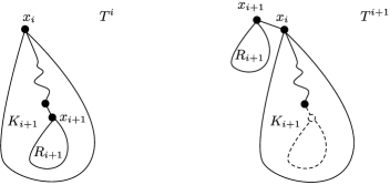
In all cases, $r(T^{m})=x_{m}$ for all $m\geq 1$. We refer to this procedure as the Aldous–Broder dynamics on $t$ and $\mathbf{x}$. One can equivalently think of the root vertex as being both the head and tail of a directed loop; then one always removes the unique edge with tail $x_{m+1}$ in $T^{m}$ and adds the directed edge $(x_{m},x_{m+1})$. Taking this perspective, let $R_{m+1}=R_{m+1}(t,\mathbf{x})$ be the subtree of $T^{m}$ rooted at $x_{m+1}$, so $R_{m+1}=T^{m}(x_{m+1})$. Let $K_{m+1}=K_{m+1}(t,\mathbf{x})$ be the other component created when removing the edge with tail $x_{m+1}$, which is empty if $x_{m+1}=x_{m}$ and otherwise contains $x_{m}$. In all cases $T^{m+1}$ is obtained from $R_{m+1}$ and $K_{m+1}$ by adding an edge from $x_{m}$ to $x_{m+1}$; see Figure 1.

Figure 1: Two successive trees $T^{i}$ and $T^{i+1}$ built from the sequence construction: $T^{i+1}$ is obtained from $T^{i}$ by cutting above $x_{i+1}$ and rearranging the parts in such a way that the subtree above the cut is appended as a child of the root $x_{i+1}$ of the subtree $R_{i+1}$ below the cut.

3.2 A modified Aldous–Broder dynamics

Say that a sequence $\mathbf{x}\in[n]^{\mathbb{N}}$ is good if for each $k\in[n]$, $\sup\{i\dvtx x_{i}=k\}=\infty$. Fix a tree $t$ on $[n]$ and a good sequence $\mathbf{x}$. We now describe a rule for removing a set of edges from $t$ to obtain an ordered forest $\mathbf{F}=\mathbf{F}(t,\mathbf{x})$ on $[n]$. [Recall that an ordered forest is an ordered sequence $(t_{1},\ldots,t_{k})$ of rooted trees.]

Figure 2: Left: a tree $t$, with node labels suppressed for readability; the first five nodes $x_{1},\ldots,x_{5}$ of some good sequence are marked in the figure. Center: the forest $\mathbf{F}(t,\mathbf{x})$ built by applying the modified Aldous–Broder dynamics to $t$ with any sequence $\mathbf{x}$ starting with $x_{1},\ldots,x_{5}$. The trees are $T_{1}(t,\mathbf{x}),\ldots,T_{4}(t,\mathbf{x})$ are shown from left to right, and $r_{1}=x_{1},r_{2}=x_{2},r_{3}=x_{4},r_{4}=x_{5}$. Right: the tree $\widehat{T}(t,\mathbf{x})$, which has root $x_{1}$.

In words, to build $\mathbf{F}(t,\mathbf{x})$ we start from the tree $t$ and make the cuts that are dictated by the sequence $\mathbf{x}$, but ignore any such cuts that fall in a subtree we have already pruned at an earlier step. Since $\mathbf{x}$ is good, we will eventually prune the root $r(t)$ and so we will ignore all but finitely many of the cuts.

Formally, let $\sigma_{0}=0$ and, for $i\geq 1$, let

$$\sigma_{i}=\inf\Biggl{\{}m>\sigma_{i-1}\dvtx x_{m}\notin\bigcup_{j=1}^{i-1}t(x_{\sigma_{j}})\Biggr{\}}.$$

Then let $\kappa=\kappa(t,\mathbf{x})=\inf\{i\dvtx x_{\sigma_{i}}=r(t)\}$. Note that we always have $\sigma_{1}=1$, that $\kappa<\infty$ since $\mathbf{x}$ is good, and that for all $j>\kappa$, $\sigma_{j}=\infty$. Recall that we write $t=(v(t),e(t))$, where $v(t)$ and $e(t)$ denote the vertex and edge set of $t$, respectively. After all the cuts in $\mathbf{x}$ have been made, we are left with a graph

$$f=\bigl{(}v(t),e(t)\setminus\bigl{\{}\bigl{(}x_{\sigma_{i}},a(x_{\sigma_{i}})\bigr{)},1\leq i\leq\kappa\bigr{\}}\bigr{)}.$$

For $1\leq i\leq\kappa$, let $T_{i}=T_{i}(t,\mathbf{x})=C(x_{\sigma_{i}},f)$. Note that $T_{i}$ is a tree, which we view as rooted at $x_{\sigma_{i}}$. We then take

$$\mathbf{F}=\mathbf{F}(t,\mathbf{x})=(T_{1},\ldots,T_{\kappa}).$$

Write $r_{i}=r_{i}(t,\mathbf{x})$ for the root of $T_{i}$ and note that $r_{\kappa}=r(t)$. Finally, write $\widehat{T}=\widehat{T}(t,\mathbf{x})$ for the tree obtained from the forest $\mathbf{F}(t,\mathbf{x})$ by adding a directed edge from the root of $T_{i+1}$ to the root of $T_{i}$, for each $i\in[\kappa-1]$, and rooted at $r_{1}$ (as suggested by the orientation of the edges). These definitions are illustrated in Figure 2. We call this procedure the modified Aldous–Broder dynamics on $t$ and $\mathbf{x}$.

The cutting procedure described above differs slightly from that used in much of the work on the subject. More precisely, it is more common to cut the tree by the removal of random edges rather than the selection of random vertices. However, there is a close correspondence between the vertex selection procedure and the edge selection procedure on a planted version of the same tree, which means results proved for one procedure have immediate analogues for the other. In particular, Janson (Janson2004 , Lemma 6.1) analyzed the difference between the two variants and showed that it is asymptotically negligible.

Now let $\mathcal{X}=(X_{m})_{m\in\mathbb{N}}$ be a sequence of i.i.d. uniform $\{1,\ldots,n\}$ random variables. It is easily seen that $\mathcal{X}$ is good with probability one. The following theorem is the key fact underlying almost all the results of the paper.

Theorem 3.1

Let $T$ be a uniform Cayley tree on $[n]$. Then for any tree $t$ on $[n]$ and any $w\in[n]$,

$${\mathbf{P}}\bigl{(}\widehat{T}(T,\mathcal{X})=t\mbox{ and }r(T)=w\bigr{)}=n^{-n}.$$

Since there are $n^{n-1}$ labeled rooted trees on $[n]$, there are $n^{n}$ possible ways to choose a labeled rooted tree on $[n]$, plus an additional vertex of said tree. In other words, the theorem states that $\widehat{T}(T,\mathcal{X})$ is a uniform Cayley tree, and that $r(T)$ is uniform on $[n]$ and independent of $\widehat{T}(T,\mathcal{X})$ (the fact that $r(T)$ is uniform on $[n]$ is immediate from the fact that $T$ is a uniform Cayley tree). Proof of Theorem 3.1 We proceed by induction on $n$, the case $n=1$ being trivial. So we now suppose that $n>1$. First, consider the case when $w=r(\widehat{T})$; we have $r(T)=r(\widehat{T})$ precisely if $X_{1}=r(T)$ and in this case $\widehat{T}=T$. Thus, for any rooted tree $t$ on $[n]$,

$${\mathbf{P}}\bigl{(}\widehat{T}=t,r(T)=r(\widehat{T})\bigr{)}={\mathbf{P}}\bigl{(}X_{1}=r(T),T=t\bigr{)}=\frac{1}{n}{\mathbf{P}}(T=t)=\frac{1}{n^{n}},$$

since $T$ is a uniform Cayley tree.

Next, fix a rooted tree $t$ on $[n]$ and any $w\in[n]$, $w\neq r(t)$. Let $c=c(t,w)$ be the child of $r=r(t)$ for which the subtree of $t$ rooted at $c$ contains the node $w$. Let $t_{r}$ and $t_{c}$ be the subtrees containing $r$ and $c$, respectively, when the edge $(c,r)$ is removed from $t$. If we are to have $r(T)=w$ and $\widehat{T}=t$, then $t_{r}$ must appear as a subtree of $T$, and we must additionally have $X_{1}=r$. Since $T$ is a uniform Cayley tree it follows that

$${\mathbf{P}}\bigl{(}r(T)=w,\widehat{T}=t\bigr{)}$$

$$\qquad={\mathbf{P}}\bigl{(}r(T)=w,\widehat{T}=t,t_{r}\mbox{ is a subtree of }T,X_{1}=r\bigr{)}$$ (1)

$$\qquad=\frac{(n-|t_{r}|)^{n-|t_{r}|}}{n^{n-1}}\cdot\frac{1}{n}\cdot{\mathbf{P}}\bigl{(}r(T)=w,\widehat{T}=t|t_{r}\mbox{ is a subtree of }T,X_{1}=r\bigr{)}.$$

Now let $\mathcal{X}^{\prime}=(X_{i}^{\prime})_{i\in\mathbb{N}}$ be the subsequence of $\mathcal{X}$ consisting of the nodes of $K_{1}(T,\mathcal{X})$, the connected component of $T$ containing the root after the edge above $X_{1}$ has been removed: for $i\in\mathbb{N}$, let

$$j_{i}=\min\bigl{\{}\ell\dvtx\bigl{|}\{X_{1},\ldots,X_{\ell}\}\cap v\bigl{(}K_{1}(T,\mathcal{X})\bigr{)}\bigr{|}=i\bigr{\}}$$

and set $X_{i}^{\prime}=X_{j_{i}}$. Given that $t_{r}$ is a subtree of $T$ and $X_{1}=r$, the entries of $\mathcal{X}^{\prime}$ are independent, uniformly random elements of $v(t_{c})$. Furthermore, under this conditioning we have that $\widehat{T}(T,\mathcal{X})=t$ and $r(T)=w$ precisely if $\widehat{T}(K_{1}(T,\mathcal{X}),\mathcal{X}^{\prime})=t_{c}$ and $r(K_{1}(T,\mathcal{X}))=w$. Since $T$ is a uniform Cayley tree and $K_{1}(T,\mathcal{X})$ is obtained from $T$ by removing the subtree rooted at $X_{1}$, it is immediate that conditional on its vertex set, $K_{1}(T,\mathcal{X})$ is again a uniform Cayley tree (and has less vertices than $T$). By induction, it follows that

$${\mathbf{P}}\bigl{(}r(T)=w,\widehat{T}=t|t_{r}\mbox{ is a subtree of }T,X_{1}=r\bigr{)}$$

$$\qquad={\mathbf{P}}\bigl{(}\widehat{T}\bigl{(}K_{1}(T,\mathcal{X}),\mathcal{X}^{\prime}\bigr{)}=t_{c},r\bigl{(}K_{1}(T,\mathcal{X})\bigr{)}=w|t_{r}\mbox{ is a subtree of }T,X_{1}=r\bigr{)}$$

$$\qquad=|t_{c}|^{-|t_{c}|}.$$

Since $|t_{c}|=n-|t_{r}|$, together with (3.2) this yields that ${\mathbf{P}}(\widehat{T}(T,\mathcal{X})=t$ and $r(T)=w)=n^{-n}$, as required.

We can transform the modified Aldous–Broder procedure for isolating the root into an edge-removal procedure, as follows. First, plant the tree to be cut at its root. Next, each time a node is selected for pruning, instead remove the parent edge incident to each selected vertex. The Aldous–Broder procedure then becomes the planted cutting procedure described in the Introduction, and $\kappa(T,\mathcal{X})$ is precisely the number of edges removed before the planted vertex is isolated. But $\kappa(T,\mathcal{X})$ is also the number of vertices on the path from $r(\widehat{T})$ to $r(T)$ in $\widehat{T}$. By Theorem 3.1, and from known results about the distance between the root and a uniformly random node in a uniform Cayley tree MeMo1978 , Kolchin1986 , Aldous1991 , Aldous1991b , Aldous1993a , the case $k=1$ of Theorem 1.1 and of Corollary 1.2 follow immediately. By a well-known bijective correspondence between labeled rooted trees with a distinguished vertex and ordered labeled rooted forests (see, e.g., AlPi1994 ), Theorem 1.3 also follows immediately (the forest consists of the sequence of trees obtained when removing the edges on the path between the root and the distinguished vertex).

Aldous Aldous1991a studied the subtree rooted at a uniformly random node in a critical, finite variance Galton–Watson tree conditioned to have size $n$. In particular, he showed that such a subtree converges in distribution to an unconditioned critical Galton–Watson tree. It is then straightforward that, for fixed $k\geq 1$, the first $k$ trees that are cut converge in distribution to a forest of $k$ critical Galton–Watson trees. On the other hand, a critical Galton–Watson tree conditioned to be large converges locally (in the sense of local weak convergence of AlSt2003 , i.e., inside balls of arbitrary fixed radius $k$ around the root) to an infinite path of nodes having a size-biased number of children (exactly one of which is again on the infinite path), where each nonpath node is the root of an unconditioned critical Galton–Watson tree. This is the incipient infinite cluster for critical, finite variance Galton–Watson trees kesten86sub . Theorem 1.3 then appears as a strengthening of this picture, valid only for Poisson Galton–Watson trees, in which $k$ is allowed to grow with $n$.

Recall that $T$ is a uniform Cayley tree on $[n]$ and that $\mathcal{X}=(X_{m})_{m\in\mathbb{N}}$ is a sequence of i.i.d. uniform elements of $[n]$. In the next proposition, which is essentially a time-reversed version of Theorem 3.1, we write $\mathbf{F}(T,\mathcal{X})=\mathbf{F}$ for readability.

Proposition 3.2

For any forest $\mathbf{f}=(t_{1},\ldots,t_{k})$ on $[n]$, given that $\mathbf{F}=\mathbf{f}$, independently for each $i\in[k-1]$ the parent $a(r(t_{i}),T)$ of $r(t_{i})$ in $T$ is a uniformly random element of $\bigcup_{j=i+1}^{k}v(t_{j})$.

If $k=1$, then there is nothing to prove. If $k>1$, then fix any sequence $\mathbf{v}=(v_{1},\ldots,v_{k-1})$ with $v_{i}\in\bigcup_{j=i+1}^{k}v(t_{j})$ for each $i\in[k-1]$. Write $t(\mathbf{f},\mathbf{v})$ for the tree formed from $\mathbf{f}$ by adding an edge from $r(t_{i})$ to $v_{i}$ for each $i\in[k-1]$. In order that $\mathbf{F}=\mathbf{f}$ and that, for each $i\in[k-1]$, $a(r(t_{i}),T)=v_{i}$, it is necessary and sufficient that $T=t(\mathbf{f},\mathbf{v})$ and that for each $i\in[k]$, $X_{\sigma_{i}}=r(t_{i})$. The probability that $T=t(\mathbf{f},\mathbf{v})$ is $n^{-(n-1)}$. Furthermore, since $(X_{m})_{m\in\mathbb{N}}$ are i.i.d. elements of $[n]$,

$${\mathbf{P}}\bigl{(}X_{\sigma_{i}}=r(t_{i}),1\leq i\leq k|T=t(\mathbf{f},\mathbf{v})\bigr{)}=\prod_{i\in[k]}\frac{1}{|\bigcup_{j\geq i}v(t_{j})|}.$$

It follows that

$${\mathbf{P}}\bigl{(}\mathbf{F}=\mathbf{f}\mbox{ and }a\bigl{(}r(t_{i}),T\bigr{)}=v_{i},1\leq i<k\bigr{)}=\frac{1}{n^{n-1}}\cdot\prod_{i\in[k]}\frac{1}{|\bigcup_{j\geq i}v(t_{j})|},$$

which proves the proposition since this expression does not depend on $v_{1},\ldots,\break v_{k-1}$.

Theorem 1.4 is an immediate consequence of Proposition 3.2.

4 Isolating more than one vertex

In this section we describe how to generalize the arguments of Section 3.2 to obtain results on isolating sets of vertices of size greater than one. Recall that when performing the planted cutting of $S$ in $t$, described in Section 1, we wrote $W=\{w_{1},\ldots,w_{k}\}$ for the set of new vertices, and wrote $M=M(t,S)$ for the (random) total number of edges removed. In order to study the random variable $M$, it turns out to be necessary to study a transformation of the planted cutting procedure. The modified procedure is defined via a canonical re-ordering of the sequence of removed edges. As such, it may be coupled with the original procedure so that the final set of removed edges is the same in both. In particular, both procedures isolate the vertices of $W$, and the total number of cuts has the same distribution in both.

In the following, for an edge $e$ and a connected component $C$, we write $e\in C$ to mean that both endpoints of $e$ lie in $C$, or equivalently (since the connected components are trees) that the removal of $e$ leaves $C$ disconnected. Also, recall from Section 2 that given a set $A$ of edges, we write $t\setminus A$ for the graph $(v(t),e(t)\setminus A)$.

Now fix a sequence $\mathbf{e}=(e_{1},\ldots,e_{m})$ of distinct edges of $t$. We say that $\mathbf{e}$ is a possible cutting sequence (for $S$ in $t$) if:

• each edge $\{v_{i},w_{i}\}$, $1\leq i\leq k$ appears in $\mathbf{e}$ ($\mathbf{e}$ really isolates $w_{1},\ldots,w_{k}$), and

• for each $1\leq j\leq m$, one has $e_{j}\in C(W,t\setminus\{e_{1},\ldots,e_{j-1}\})$, that is, each $e_{j}$ indeed produces a cut.

We now describe a canonical re-ordering of $\mathbf{e}$, which we denote $\mathbf{e}^{*}$; this re-ordering operation gives rise to the modified cutting procedure. In $\mathbf{e}^{*}$, we first list all edges whose removal decreases the size of the component containing $w_{1}$ (in increasing order of arrival time). We then list all remaining edges whose removal decreases the size of the component containing $w_{2}$, again in increasing order of arrival time, and so on. (This is somewhat related to a size-biased reordering of an exchangeable random structure; see Pitman2006 , Chapter 1. The next three paragraphs formalize this description.)

For $1\leq i\leq k$, write

$$U_{i}=U_{i}(\mathbf{e})=\bigl{\{}j\dvtx e_{j}\in C\bigl{(}w_{i},t\setminus\{e_{1},\ldots,e_{j-1}\}\bigr{)}\bigr{\}}$$

and let $U_{i}^{*}=U_{i}\setminus(\bigcup_{j=1}^{i-1}U_{j})$. In words, $U_{i}^{*}$ is the set of times $j$ at which the component containing $w_{i}$ does not contain any of $w_{1},\ldots,w_{i-1}$, and such that removing the current edge $e_{j}$ decreases the size of this component.

Next, let $m(i)=m(i,t,\mathbf{e})=|U_{i}|$, write $Z_{i}=Z_{i}(\mathbf{e})=(z_{i,1},\ldots,z_{i,m(i)})$ for the sequence obtained by listing the elements of $U_{i}$ in increasing order, and define $Z_{i}^{*}$ accordingly. Notice that once $w_{i}$ is in a component distinct from $w_{1},\ldots,w_{i-1}$, it can never rejoin such a component, and so writing $s(i)=s(i,t,\mathbf{e})=\min\{\ell\dvtx z_{i,\ell}\in U_{i}^{*}\}$, we must have

$$Z_{i}^{*}=(z_{i,s(i)},z_{i,s(i)+1},\ldots,z_{i,m(i)}).$$

We then write

$$\mathbf{e}^{*} = (e_{z_{1,s(1)}},\ldots,e_{z_{1,m(1)}},e_{z_{2,s(2)}},\ldots,e_{z_{2,m(2)}},\ldots,e_{z_{k,s(k)}},\ldots,e_{z_{k,m(k)}})$$

$$= \bigl{(}e_{1}^{*},\ldots,e_{m}^{*}\bigr{)},$$

the latter equality constituting the definition of $e_{1}^{*},\ldots,e_{m}^{*}$. For $1\leq i\leq k$, let $a_{i}(t,\mathbf{e}^{*})=1+\sum_{\ell=1}^{i-1}(m(\ell)-s(\ell)+1)$ let $b_{i}(t,\mathbf{e}^{*})=\sum_{\ell=1}^{i}(m(\ell)-s(\ell)+1)$, and set

$$\mathbf{e}^{*}_{i}=\bigl{(}e^{*}_{j},a_{i}\leq j\leq b_{i}\bigr{)}=\bigl{(}e_{z_{i,j}},s(i)\leq j\leq m(i)\bigr{)}.$$

We remark that necessarily $e_{z_{i,m(i)}}=\{w_{i},v_{i}\}$, and so in particular the sequence $\mathbf{e}^{*}_{i}$ is nonempty for each $1\leq i\leq k$.

Now write $\mathbf{E}=\mathbf{E}(t,S)=(E_{1},\ldots,E_{M})$ for the random sequence of removed edges (in the original planted cutting procedure), write $\mathbf{E}^{*}=\break\mathbf{E}^{*}(t,S)=(E_{1}^{*},\ldots,E_{M}^{*})$ for the rearrangement of $\mathbf{E}$ described above, and likewise define $\mathbf{E}^{*}_{i}$, for $1\leq i\leq k$, as above.

It is easily seen that if $\mathbf{e}$ is not a possible cutting sequence, then ${\mathbf{P}}(\mathbf{E}(t,S)=\mathbf{e})=0$, and if $\mathbf{e}$ is a possible cutting sequence, then

$${\mathbf{P}}\bigl{(}\mathbf{E}(t,S)=\mathbf{e}\bigr{)} = \prod_{j=1}^{m}\frac{1}{|e(C(W,t\setminus\{e_{1},\ldots,e_{j-1}\}))|}.$$ (2)

For our purposes, it is in fact the expression for ${\mathbf{P}}(\mathbf{E}^{*}(t,S)=\mathbf{e}^{*})$ given in the following lemma that will be more useful. Fix any sequence $\mathbf{f}=(f_{1},\ldots,f_{m})$ of edges of $t\langle S\rangle$. If there exists a possible cutting sequence $\mathbf{e}=(e_{1},\ldots,e_{m})$ for $S=(v_{1},\ldots,v_{k})$ in $t$ such that $\mathbf{e}^{*}=\mathbf{f}$, then we say that $\mathbf{f}$ is valid (for $t$ and $S$).

Lemma 4.1

Given any sequence $\mathbf{f}=(f_{1},\ldots,f_{m})$ that is valid for $t$ and $S$, we have

$${\mathbf{P}}\bigl{(}\mathbf{E}^{*}(t,S)=\mathbf{f}\bigr{)}=\prod_{i=1}^{k}\prod_{j=a_{i}(t,\mathbf{f})}^{b_{i}(t,\mathbf{f})}\frac{1}{|e(C(w_{i},t\setminus\{f_{1},\ldots,f_{j-1}\}))|}.$$

We prove the lemma by induction on $|e(t\langle S\rangle)|$. Fix $\mathbf{f}$ as in the statement of the lemma, write

$$\mathcal{E}(\mathbf{f})=\mathcal{E}(\mathbf{f},t,S)=\bigl{\{}\mathbf{e}\dvtx\mathbf{e}\mbox{ is a possible cutting sequence for $S$ in $t$ and }\mathbf{e}^{*}=\mathbf{f}\bigr{\}}$$

and note that $\mathbf{f}\in\mathcal{E}(\mathbf{f})$. For any $\mathbf{e}=(e_{1},\ldots,e_{m})\in\mathcal{E}(\mathbf{f})$ we necessarily have $e_{1}=f_{1}$, and so

$${\mathbf{P}}\bigl{(}\mathbf{E}_{1}^{*}(t,S)=f_{1}\bigr{)}={\mathbf{P}}\bigl{(}\mathbf{E}_{1}(t,S)=f_{1}\bigr{)}=\frac{1}{|e(t\langle S\rangle)|}.$$

If $e_{1}=\{v_{1},w_{1}\}$, then writing $S^{\prime}=(v_{2},\ldots,v_{k})$, we have

$${\mathbf{P}}\bigl{(}\mathbf{E}^{*}=\mathbf{f}|\mathbf{E}^{*}_{1}=f_{1}\bigr{)} = {\mathbf{P}}\bigl{(}\mathbf{E}^{*}=\mathbf{f}|\mathbf{E}_{1}=f_{1}\bigr{)}$$

$$= {\mathbf{P}}\bigl{(}\mathbf{E}^{*}\bigl{(}t,S^{\prime}\bigr{)}=(f_{2},\ldots,f_{m})\bigr{)}$$

and the result follows by induction since $t\langle S^{\prime}\rangle$ has fewer edges than $t\langle S\rangle$.

If $e_{1}\neq\{v_{1},w_{1}\}$, then write $t_{1}=C(w_{1},t\langle S\rangle\setminus\{e_{1}\})$, and write $t_{2}$ for the other component of $t\langle S\rangle\setminus\{e_{1}\}$; each of these trees has fewer edges than $t\langle S\rangle$. Write $S_{1}=(x_{1},\ldots,x_{k_{1}})$ and $S_{2}=(y_{1},\ldots,y_{k_{2}})$ for the nodes of $S$ within $t_{1}$ and $t_{2}$, respectively, listed in the same order as in $S$.

Now fix any possible cutting sequence $\mathbf{e}=(e_{1},\ldots,e_{m})$ with $e_{1}=f_{1}$. Write $\mathbf{e}^{(1)}$ and $\mathbf{e}^{(2)}$ for those edges in the sequence $(e_{2},\ldots,e_{m})$ falling in $t_{1}$ and $t_{2}$, respectively, and listed in the same order as in $\mathbf{e}$. Then it is clear that, conditionally on $\mathbf{E}_{1}=f_{1}$, the sequences $\mathbf{E}(t_{1},S_{1})$ and $\mathbf{E}(t_{2},S_{2})$ have the distribution of the planted cutting procedure on $t_{1}\langle S_{1}\rangle$ and $t_{2}\langle S_{2}\rangle$, respectively, and are independent. In other words,

$$\mathbf{P}\bigl{(}\mathbf{E}(t_{1},S_{1})=\mathbf{e}^{(1)},\mathbf{E}(t_{2},S_{2})=\mathbf{e}^{(2)}|\mathbf{E}_{1}=f_{1}\bigr{)}$$

$$\qquad={\mathbf{P}}\bigl{(}\mathbf{E}(t_{1},S_{1})=\mathbf{e}^{(1)}\bigr{)}\cdot{\mathbf{P}}\bigl{(}\mathbf{E}(t_{2},S_{2})=\mathbf{e}^{(2)}\bigr{)}.$$

Furthermore, if $\mathbf{e}\in\mathcal{E}(\mathbf{f})$, then $e_{1}=f_{1}$, and $\mathbf{e}\in\mathcal{E}(\mathbf{f})$ if and only if $\mathbf{e}^{(1)}\in\mathcal{E}(\mathbf{f}^{(1)},t_{1},S_{1})$ and $\mathbf{e}^{(2)}\in\mathcal{E}(\mathbf{f}^{(2)},t_{2},S_{2})$. [Note: this does not mean that the map from $\mathbf{e}$ to $(\mathbf{e}^{(1)},\mathbf{e}^{(2)})$ is bijective! In fact, for a given pair $\mathbf{e}^{(1)}\in\mathcal{E}(\mathbf{f}^{(1)},t_{1},\break S_{1})$ and $\mathbf{e}^{(2)}\in\mathcal{E}(\mathbf{f}^{(2)},t_{2},S_{2})$, the number of pre-images in $\mathcal{E}(\mathbf{f})$ is precisely ${m-1\choose m_{1}}$, where $m_{1}$ is the length of $\mathbf{f}^{(1)}$.] Also, $\mathbf{f}^{(1)}$ (resp., $\mathbf{f}^{(2)}$) is valid for $t_{1}$ and $S_{1}$ (resp., for $t_{2}$ and $S_{2}$). It follows that

$${\mathbf{P}}\bigl{(}\mathbf{E}^{*}=\mathbf{f}|\mathbf{E}_{1}=f_{1}\bigr{)}$$

$$\quad=\sum_{\mathbf{e}\in\mathcal{E}}{\mathbf{P}}(\mathbf{E}=\mathbf{e}|\mathbf{E}_{1}=f_{1})$$

$$\quad=\sum_{\mathbf{e}^{(1)}\in\mathcal{E}(\mathbf{f}^{(1)},t_{1},S_{1})}\sum_{\mathbf{e}^{(2)}\in\mathcal{E}(\mathbf{f}^{(2)},t_{2},S_{2})}{\mathbf{P}}\bigl{(}\mathbf{E}(t_{1},S_{1})=\mathbf{e}^{(1)},\mathbf{E}(t_{2},S_{2})=\mathbf{e}^{(2)}|\mathbf{E}_{1}=f_{1}\bigr{)}$$

$$\quad=\sum_{\mathbf{e}^{(1)}\in\mathcal{E}(\mathbf{f}^{(1)},t_{1},S_{1})}\sum_{\mathbf{e}^{(2)}\in\mathcal{E}(\mathbf{f}^{(2)},t_{2},S_{2})}{\mathbf{P}}\bigl{(}\mathbf{E}(t_{1},S_{1})=\mathbf{e}^{(1)}\bigr{)}\cdot{\mathbf{P}}\bigl{(}\mathbf{E}(t_{2},S_{2})=\mathbf{e}^{(2)}\bigr{)}$$

$$\quad={\mathbf{P}}\bigl{(}\mathbf{E}^{*}(t_{1},S_{1})=\mathbf{f}^{(1)}\bigr{)}\cdot{\mathbf{P}}\bigl{(}\mathbf{E}^{*}(t_{2},S_{2})=\mathbf{f}^{(2)}\bigr{)}$$

from which the result again follows by induction.

The formula in the preceding lemma implies that removing edges in the order given by $\mathbf{E}^{*}$ corresponds to the following procedure. For each $1\leq i\leq k$, in that order, remove edges of $t$ uniformly at random from among those whose removal reduces the size of the component currently containing $w_{i}$, until $w_{i}$ is isolated. We call this the ordered cutting of $S$ in $t$.

For $1\leq i\leq k$, write $M_{i}$ for the random time at which $w_{i}$ is isolated in the ordered cutting procedure

$$M_{i} = M_{i}(t,S)=\max\bigl{\{}j\dvtx E_{j}^{*}\in C\bigl{(}w_{i},t\setminus\bigl{\{}E_{1}^{*},\ldots,E_{j-1}^{*}\bigr{\}}\bigr{)}\bigr{\}}$$

$$= \min\bigl{\{}j\dvtx\bigl{|}C\bigl{(}w_{i},t\setminus\bigl{\{}E_{1}^{*},\ldots,E_{j}^{*}\bigr{\}}\bigr{)}\bigr{|}=0\bigr{\}}$$

(recall that the counting does not include planted vertices), and note that $M_{1}<M_{2}<\cdots<M_{k}\stackrel{{\scriptstyle d}}{{=}}M$.

Now, let $T$ be a uniform Cayley tree on $[n]$, let $V_{1},\ldots,V_{k}$ be independent, uniformly random elements of $[n]$, and let $S_{k}=(V_{1},\ldots,V_{k})$. Then write $M_{k}=M(T,S_{k})$ for the number of edges removed during the ordered cutting of $S_{k}$ in $t$.

Theorem 4.2

$M_{k}-k$ is distributed as the number of edges spanned by the root plus $k$ independent, uniformly random nodes in a uniform Cayley tree of size $n$.

Theorem 1.1 follows immediately from Theorem 4.2 and the relationship between planted cutting and ordered cutting described above. To prove Theorem 4.2, we will exhibit a coupling which generalizes that of Section 3.2 and which we now explain. The coupling hinges upon the following, easy lemma, whose proof is omitted. Recall that if $S$ is a set of nodes in a tree $t$, then $t{[\![S]\!]}$ is the subtree of $S$ spanned by $S$.

Lemma 4.3

Fix $i\geq 1$. Let $T$ be a uniform Cayley tree on $[n]$, let $V_{1},\ldots,V_{i+1}$ be independent, uniformly random elements of $[n]$, and let $S=\{r(T),V_{1},\ldots,V_{i}\}$. Let $U$ be the most recent ancestor of $V_{i+1}$ in $T$ which is an element of $v(T{[\![S]\!]})$. Let $R$ be the set of nodes whose path to $V_{i+1}$ uses no edges of $T{[\![S]\!]}$ (such paths may pass through $U$). Let $T^{+}=T{[\![R]\!]}$, let $T^{-}=T{[\![([n]\setminus R)\cup\{U\}]\!]}$ and root $T^{+}$ and $T^{-}$ at $U$ and at $r(T)$, respectively. Then conditionally on $R$, $T^{+}$ is a uniformly random labeled rooted tree on $R$, independent of $T^{-}$ and of $V_{1},\ldots,V_{i}$, and $V_{i+1}$ is a uniformly random element of $R$ independent of $T^{+},T^{-}$ and $V_{1},\ldots,V_{i}$.

The definitions in Lemma 4.3 are depicted in Figure 3.

Figure 3: An example of the definitions of Lemma 4.3 in the case $i=2$ [so $S=(r(T),V_{1},V_{2})$]. The subtree $T{[\![S]\!]}$ is in thicker black lines. The tree $T^{+}$ is in thick grey lines, and the tree $T^{-}$ consists of all black lines (thick and thin).

Proof of Theorem 4.2 We provide a coupling between the random sequence of edges $\mathbf{E}^{*}(T,(V_{1},\ldots,V_{k}))$ and a sequence $T_{1},\ldots,T_{k}$ of trees on $[n]$, such that the following properties hold. First, for any rooted tree $t$ on $[n]$, and any $v_{1},\ldots,v_{i}$ elements of $[n]$ (not necessarily distinct),

$${\mathbf{P}}(T_{i}=t,V_{1}=v_{1},\ldots,V_{i}=v_{i})=n^{-(n-1+i)}.$$ (3)

Second, for each $1\leq i\leq k$, the following holds:

• [($\star$)]

• the forest obtained from $T\langle(V_{1},\ldots,V_{i})\rangle$ by first removing all edges of $\{E^{*}_{1},\ldots,E^{*}_{M_{i}}\}$, then deleting $w_{1},\ldots,w_{i}$, is identical to the forest obtained from $T_{i}$ by removing all edges of its subtree $T_{i}{[\![r(T_{i}),V_{1},\ldots,V_{i}]\!]}$.

Equation (3) says that $T_{i}$ is a uniform Cayley tree and $V_{1},\ldots,V_{i}$ are independent of $T_{i}$, and ($\star$) then implies in particular (by considering only the case $i=k$) that $M_{k}-k$ is equal to the number of edges of $T_{k}{[\![r(T_{k}),V_{1},\ldots,V_{k}]\!]}$. This clearly implies the theorem, and so it remains to explain how we construct such a sequence.

Fix a sequence $\mathcal{X}=(X_{i})_{i\geq 1}$ of i.i.d. uniform elements of $[n]$. Let $T_{1}$ be the tree built by running the modified Aldous–Broder dynamics on $T^{r\leftrightarrow V_{1}}$ (recall that this is the tree $T$, rerooted at node $V_{1}$) with the sequence $(X_{i})_{i\geq 1}$. [In the notation of Section 3.2, $T_{1}=\widehat{T}(T^{r\leftrightarrow V_{1}},\mathcal{X})$.] By Theorem 3.1, for any tree $t$ on $[n]$ and any $v\in[n]$, ${\mathbf{P}}(T_{1}=t,V_{1}=v)=n^{-n}$, so (3) holds in the case $i=1$. Temporarily write $u_{1},\ldots,u_{\ell}$ for the nodes on the path in $T_{1}$ from $r(T_{1})$ to $V_{1}$, in the same order they appear on that path. We must then have $u_{\ell}=V_{1}$, and $M_{1}=\ell$. For $1\leq j\leq\ell-1$, let $E_{j}^{*}=\{u_{j},a(u_{j},T^{r\leftrightarrow V_{1}})\}$, and note that this is also an edge of $T$ since $T$ and $T^{r\leftrightarrow V_{1}}$ have the same edge set. Then let $E_{M_{1}}^{*}=\{u_{\ell},w_{1}\}=\{V_{1},w_{1}\}$. (An example of this construction is shown in Figure 4.) By construction, it is immediate that ($\star$) then holds in the case $i=1$.

Figure 4: Left: the tree $T\langle(V_{1})\rangle$. Center: the tree $T^{r\leftrightarrow V_{1}}$, planted at $V_{1}$. Right: the tree $T_{1}$. The vertex and edge labels provide an example of the construction in the proof of Theorem 4.2, in the case $k=1$. For each of the three trees, the forest obtained by removing the bold edges [and, for $T\langle(V_{1})\rangle$, then throwing away the vertex $w_{1}$] is identical.

Now fix $1\leq j<k$, suppose that $T_{1},\ldots,T_{j}$ and $(E_{1}^{*},\ldots,E_{M_{j}}^{*})$ are already defined and that (3) and $(\star)$ both hold for each $1\leq i\leq j$. As defined, $V_{j+1}$ is independent of $T_{i}$ and of $(E_{1}^{*},\ldots,E_{M_{j}}^{*})$, and so for any tree $t$ on $[n]$ and any sequence $u_{1},\ldots,u_{j+1}$ of elements of $[n]$, we have

$${\mathbf{P}}(T_{j}=t,V_{1}=u_{1},\ldots,V_{j+1}=u_{j+1})=n^{-(n-1+i+1)}.$$ (4)

Let $U$ be the most recent ancestor of $V_{j+1}$ that lies in $T_{j}{[\![r(T_{i}),V_{1},\ldots,V_{j}]\!]}$, and define $T^{+}$ and $T^{-}$ as in Lemma 4.3.

Now let $\mathcal{X}^{\prime}$ be a random sequence such that conditionally on $v(T^{+})$, the entries of $\mathcal{X}^{\prime}$ are independent uniform elements of $v(T^{+})$, independent of all preceding randomness. Then apply the modified Aldous–Broder dynamics to $T^{+,r\leftrightarrow V_{j+1}}$, and call the result $T^{*}$. By Theorem 3.1, given that $v(T^{+})=S$, $(T^{+},V_{j+1})$ and $(T^{*},V_{j+1})$ are identically distributed. As above, let $u_{1},\ldots,u_{\ell}$ be the nodes on the path from $r(T^{*})$ to $V_{j+1}$, and note that we must have $M_{j+1}=M_{j}+\ell$. For $1\leq i\leq\ell-1$ let $E^{*}_{M_{i}+j}=\{u_{i},a(u_{i},T^{+,r\leftrightarrow V_{j+1}})\}$, and let $E^{*}_{M_{j+1}}=\{V_{j+1},w_{j+1}\}$. In words, we have applied exactly the same construction as in the case $i=1$, but to the subtree $T^{+}$ of $T$ (which contains $V_{j+1}$). Figures 3 and 4 may be useful as visual aids to these definitions.

Write $P$ for the parent of $U$ in $T_{j}$, and $C_{1},\ldots,C_{\ell}$ for the children of $U$ in $T_{j}\setminus T^{+}$ (any such child is an ancestor of at least one of $V_{1},\ldots,V_{j}$). Now let $T_{j+1}$ be the tree obtained from $T_{j}$ by replacing $T^{+}$ by $T^{*}$. In other words, $T_{j+1}$ is built from $T_{j}$ by, first, removing all edges of $T_{j}$ that are incident to nodes of $T^{+}$ and then, second, adding all edges of $T^{*}$ as well as edges from the root of $T^{*}$ to $P$ and to each of $C_{1},\ldots,C_{\ell}$. With this construction, $(\star)$ now holds for all $1\leq i\leq j+1$.

Finally, write $R=v(T^{+})$. By Lemma 4.3 and by Theorem 3.1, $(T^{+},V_{j+1})$ and $(T^{*},V_{j+1})$ are identically distributed conditionally on their vertex sets, and both are independent of $T^{-}$ and of $V_{1},\ldots,V_{j}$. It follows that (4) still holds with $T_{j}$ replaced by $T_{j+1}$, and this verifies (3) and completes the proof by induction.

5 A novel transformation of the Brownian CRT

In Janson2006c , Janson suggested that it should be possible to define a version of the cutting procedure directly on $\mathcal{T}$. In this section, we provide such a construction. This construction yields straightforward, “conceptual” proofs of some of the main results of Janson2006c , and also provides a novel, reversible transformation from $\mathcal{T}$ to another, doubly-rooted Brownian CRT. (We remark in passing that the results of this section can also be straightforwardly used to prove the first convergence result from Theorem 1.10 of Janson2006c .) Using the by now well-known coding of the Brownian CRT by a standard Brownian excursion, this transformation can be viewed as a new, invertible random transformation between Brownian excursion and Brownian Bridge.

We now describe the details of the construction, using the language of $\mathbb{R}$-trees. For the interested reader, we describe the corresponding transformation from Brownian excursion to reflecting Brownian bridge in Appendix B.

We begin with a quick, high-level description of the transformation. An initial compact real tree $\mathcal{T}$ distributed as the Brownian CRT will be cut by points falling on its skeleton. When a point arrives, the current tree is separated into two connected components; the one containing the root will suffer further cuts at later times, while the other one—the pruned tree—will no longer be cut. As in the discrete transformation of Section 3.2, the cut trees are rearranged by attaching their roots to a “backbone” so as to form a new real tree. We now describe the continuous transformation by first building the backbone that will eventually connect the roots of the pruned subtrees, and then specifying where these subtrees should be grafted along the backbone.

5.1 The details of the transformation

Let $\mathcal{P}$ be a Poisson process on $\operatorname{skel}(\mathcal{T})\times[0,\infty)$ with intensity measure $\ell\otimes dt$, and for each $t\geq 0$, let

$$\mathcal{P}^{\circ}_{t}=\bigl{\{}x\in\mathcal{T}\dvtx\exists s,0\leq s\leq t,(x,s)\in\mathcal{P}\bigr{\}}.$$

In aldous1998standard , Aldous and Pitman used the point process $\mathcal{P}$ to construct (what is now called) a self-similar fragmentation process on $\mathcal{T}$ Bertoin2006 . For each $t\geq 0$, let $\mathcal{F}^{\circ}_{t}=\mathcal{T}\setminus\mathcal{P}^{\circ}_{t}$. In particular, two points $u,v\in\mathcal{T}\setminus\mathcal{P}^{\circ}_{t}$ are in the same component of $\mathcal{F}^{\circ}_{t}$ precisely if, in $\mathcal{T}$, the path ${[\![u,v]\!]}$ contains no element of $\mathcal{P}^{\circ}_{t}$. Aldous and Pitman aldous1998standard established many beautiful facts about how the collection of masses of the components of $\mathcal{F}^{\circ}_{t}$ evolve with $t$; one basic fact from aldous1998standard is that a.s., for each $t>0$, $\mathcal{F}^{\circ}_{t}$ has only countably many components, and the total mass of all components of $\mathcal{F}^{\circ}_{t}$ is one. (This seems intuitively obvious, but note that it is a priori possible that for every $t>0$, $\mathcal{F}^{\circ}_{t}$ contains uncountably many components, each of mass zero; consider $[0,1]\setminus\mathbb{Q}$.)

For $t\geq 0$, write $\widetilde{\mathcal{T}}_{t}$ for the component of $\mathcal{F}^{\circ}_{t}$ containing the root $\rho$ at time $t$; then define a process $(L(t),t\geq 0)$ by setting

$$L(t)=\int_{0}^{t}\mu(\widetilde{\mathcal{T}}_{s})\,ds.$$ (5)

The process $L(t)$ is the continuum analogue of the “number of cuts by time $t$”; the process $(L(t),t\geq 0)$ will code the distance along the backbone in the continuum transformation; see Theorem 5.5 and Corollary 5.6 below.

Theorem 6 of aldous1998standard states that if we define an increasing function $(X(t),t\geq 0)$ by

$$\bigl{(}\mu(\widetilde{\mathcal{T}}_{t}),t\geq 0\bigr{)}=\frac{1}{1+X(t)},$$ (6)

then $X(\cdot)$ is a stable subordinator of index $1/2$, or in other words, is distributed as the inverse local time process at zero of a standard reflecting Brownian motion. The function $X(\cdot)$ has almost sure quadratic growth, and it follows that $L(\infty):=\lim_{t\to\infty}L(t)$ is almost surely finite. [The proof of Corollary 5.6, below, contains a different proof that $L(\infty)$ is almost surely finite, using the principle of accompanying laws.]

Since $\mathcal{P}$ is a countable set, we may enumerate its atoms as $((p_{i},\tau_{i}),i\in\mathbb{N})$. For $t\geq 0$, let

$$I_{t}=\bigl{\{}i\in\mathbb{N}\dvtx 0\leq\tau_{i}\leq t,\mu(\widetilde{\mathcal{T}}_{\tau_{i}})<\mu(\widetilde{\mathcal{T}}_{\tau_{i}-})\bigr{\}}$$

and let

$$\mathcal{P}_{t}=\{p_{i}\dvtx i\in I_{t}\}\subseteq\mathcal{P}^{\circ}_{t}.$$

Let $P_{\infty}=\bigcup_{t\geq 0}\mathcal{P}_{t}$, and let $I_{\infty}=\bigcup_{t\geq 0}I_{t}$. Next, for $0\leq t\leq\infty$, let $\widetilde{\mathcal{F}}_{t}=\mathcal{T}\setminus\mathcal{P}_{t}$, let $\tilde{d}_{t}$ be its intrinsic distance: for points $x,y$ in the same component of $\widetilde{\mathcal{F}}_{t}$, we have $\tilde{d}_{t}(x,y)=d(x,y)$, while for $x,y$ in distinct components of $\widetilde{\mathcal{F}}_{t}$, we have $\tilde{d}_{t}(x,y)=\infty$, and let $\tilde{\mu}_{t}$ be the restriction of $\mu$ to $\widetilde{\mathcal{F}}_{t}$. Then let $(\mathcal{F}_{t},d_{t})$ be the metric space completion of $(\widetilde{\mathcal{F}}_{t},\tilde{d}_{t})$, and let $\mu_{t}$ be the extension of $\tilde{\mu}_{t}$ obtained by assigning measure zero to all points of $\mathcal{F}_{t}\setminus\widetilde{\mathcal{F}}_{t}$; note that there are only countably many such points.

Next, write $\mathcal{T}_{t}$ for the component of $\mathcal{F}_{t}$ containing $\rho$. We then have that a.s. for all $t\geq 0$, $\widetilde{\mathcal{T}}_{t}$ is a connected component of $\widetilde{\mathcal{F}}_{t}$, and that a.s.

$$\bigl{(}\mu(\widetilde{\mathcal{T}}_{t}),t\geq 0\bigr{)}=\bigl{(}\mu_{t}(\mathcal{T}_{t}),t\geq 0\bigr{)}.$$ (7)

By definition, a.s. for every $0\leq s<t$, every component of $\widetilde{\mathcal{F}}_{s}$ not containing $\rho$ is also a component of $\widetilde{\mathcal{F}}_{t}$. This naturally extends to the completions $\mathcal{F}_{s}$ and $\mathcal{F}_{t}$.

For $0\leq t\leq\infty$, let $\tilde{\phi}_{t}$ be the identity map from $\widetilde{\mathcal{F}}_{t}$ to $\mathcal{T}$, and let $\phi_{t}$ be the unique extension of $\tilde{\phi}_{t}$ to $\mathcal{F}_{t}$ whose restriction to any component of $\mathcal{F}_{t}$ is a continuous function. With probability one, for each $i\in I_{\infty}$, $p_{i}$ has degree two in $\mathcal{T}$ and also in $\mathcal{F}_{\tau_{i}-}$. It follows that almost surely, for each $i\in I_{\infty}$, $\mathcal{F}_{\tau_{i}}\setminus\mathcal{F}_{\tau_{i}-}$ contains precisely two points. Call these points $x_{i}$ and $y_{i}$, labeled so that $x_{i}\notin\mathcal{T}_{\tau_{i}}$ and $y_{i}\in\mathcal{T}_{\tau_{i}}$. Write $f_{i}$ for the component of $\mathcal{F}_{\tau_{i}}$ containing $x_{i}$. Necessarily, $x_{i}\in f_{i}\setminus\widetilde{\mathcal{F}}_{t}$ and $p_{i}=\phi_{t}(x_{i})$ is the closest point of $\phi_{t}(f_{i})$ to $\rho$; in other words, $p_{i}$ is “the root of the subtree cut at time $\tau_{i}$.” Also, $x_{i}$ and $y_{i}$ are both leaves in $\mathcal{F}_{\tau_{i}}$. For distinct points $p_{i},p_{j}\in I_{t}$ the trees $f_{i},f_{j}$ are disjoint, so in particular $x_{i}\neq x_{j}$.

The space $(\mathcal{F}_{\infty},d_{\infty},\mu_{\infty})$ is the limiting analogue of the forest $\mathbf{F}$ from Section 3.2. We note that $(\mathcal{T},\mu)$ can be recovered from $(\mathcal{F}_{\infty},d_{\infty},\mu_{\infty})$ by identifying $x_{i}$ and $y_{i}$ for each $p_{i}\in I_{\infty}$, and taking as measure the corresponding push-forward of $\mu_{\infty}$.

For $0\leq t\leq\infty$, let $A_{t}$ be the real tree consisting of the line segment $[0,L(t)]$ with the standard distance. Then form a measured $\mathbb{R}$-tree $(\widehat{\mathcal{T}}_{t},\hat{d}_{t},\hat{\mu}_{t})$ from $A_{t}$ and $\mathcal{F}_{t}\setminus\mathcal{T}_{t}$, by identifying $x_{i}\in f_{i}$ and $L(\tau_{i})\in[0,L(t)]$, for each $i\in I_{t}$, with measure $\hat{\mu}_{t}$ given by the push-forward of $\mu_{t}|_{\mathcal{F}_{t}\setminus\mathcal{T}_{t}}$. [We justify that $(\widehat{\mathcal{T}}_{t},\hat{d}_{t},\hat{\mu}_{t})$ is indeed a well-defined random $\mathbb{R}$-tree, using a coding by excursions, in Appendix B.] We naturally view these spaces as increasing in $t$. Write $\widehat{\mathcal{T}}=\widehat{\mathcal{T}}_{\infty}$, $\hat{d}=\hat{d}_{\infty}$, $\hat{\mu}=\hat{\mu}_{\infty}$ and let $u=L(0)$ and $v=L(\infty)$. Almost surely both $u$ and $v$ are elements of $\widehat{\mathcal{T}}$.

The set of points of ${[\![u,v]\!]}$ of degree greater than two in $(\widehat{\mathcal{T}},\hat{d})$ are precisely the images in $\widehat{\mathcal{T}}$ of the points $\{x_{i},i\in I_{\infty}\}$ in $\mathcal{F}_{\infty}$, and if $x$ is the image of such a point $x_{i}$, then $\hat{d}(u,x)=L(\tau_{i})$. It follows that the set of times $\{\tau_{i},i\in I_{\infty}\}$ is measurable with respect to $(\widehat{\mathcal{T}},\hat{d},\hat{\mu})$. Also, a.s. $\{y_{i},i\in I_{\infty}\}\cap\{x_{i},i\in I_{\infty}\}=\varnothing$, so none of the points $\{y_{i},i\in I_{\infty}\}$ are identified with other points when forming $\widehat{\mathcal{T}}$. In other words, we may view the points $\{y_{i},i\in I_{\infty}\}$ as points of $\widehat{\mathcal{T}}$ (rather than as members of equivalence classes of points).

Now recall the definition of $(\mathcal{T},d,\mu,\rho)$ from the start of the section, and let $\rho^{\prime}$ be a point of $\mathcal{T}$ selected according to $\mu$ and independent of $\rho$.

Theorem 5.1

It holds that $(\widehat{\mathcal{T}},\hat{d},\hat{\mu},(u,v))$ has the same distribution as $(\mathcal{T},d,\mu,(\rho,\rho^{\prime}))$. Furthermore, conditionally on $(\widehat{\mathcal{T}},\hat{d},\hat{\mu},(u,v))$, the elements of $\{y_{i},i\in I_{\infty}\}$ are mutually independent, and for all $i\in I_{\infty}$, $y_{i}$ is distributed according to the probability measure $\hat{\mu}|_{\widehat{\mathcal{T}}\setminus\widehat{\mathcal{T}}_{\tau_{i}}}/(1-\hat{\mu}(\widehat{\mathcal{T}}_{\tau_{i}}))$.

We remark that Theorem 1.5 is an immediate consequence of the first assertion of the theorem. Likewise, Theorem 1.7 immediately follows from the definitions of $(\widehat{\mathcal{T}},\hat{d},\hat{\mu},(u,v))$ and of the points $\{y_{i},i\in I_{\infty}\}$ and from the second assertion of the theorem.

The remainder of Section 5 is devoted to the proof of Theorem 5.1. The proof of Theorem 5.1 relies on couplings with the construction for uniform Cayley trees, and we introduce these couplings in Section 5.2. In Section 5.3, we show that the process $(L(t),t\geq 0)$ is indeed the correct analogue of “number of cuts” in the discrete setting. Finally, we wrap up the proof of Theorem 5.1 in Section 5.4.

5.2 Some couplings between discrete and continuous trees

The couplings we introduce in this section are not specific to the case of uniform Cayley trees. This will be important in Section 6, when we extend our results to other finite-variance critical conditioned Galton–Watson trees.

Let $\xi=(\xi_{i},i\geq 0)$ be a critical finite-variance offspring distribution, that is, a probability distribution on $\{0,1,\ldots\}$ with

$$\sum_{i\geq 0}i\xi_{i}=1\quad\mbox{and}\quad\sigma^{2}=\sum_{i\geq 0}i(i-1)\xi_{i}\in(0,\infty).$$

In the following, we consider only values of $n$ such that a sum of $n$ i.i.d. random variables with distribution $\xi$ equals $n-1$ with positive probability. For such $n\geq 1$, let $T^{n}$ be a Galton–Watson tree with offspring distribution $\xi$, conditioned to have $n$ nodes. For $x,y\in T^{n}$ let $d^{n}(x,y)$ be $\sigma n^{-1/2}$ times the graph distance between $x$ and $y$ in $T^{n}$. Let $\rho^{n}$ denote the root of $T^{n}$, let $\mu^{n}$ be the measure placing mass $1/n$ on each node of $T^{n}$ and let $\ell^{n}$ be the measure placing mass $\sigma n^{-1/2}$ on each vertex of $T^{n}$ (the “discrete, rescaled length measure”). Let next, $\mathcal{T}$ be the Brownian CRT with root $\rho$ and distance metric $d$, let $\mu$ be its mass measure and let $\ell$ be the length measure on the skeleton of $\mathcal{T}$. We will use the following fundamental result heavily.

Theorem 5.2 ((Aldous Aldous1993a , Le Gall legall06realtrees ))

It holds that

$$\bigl{(}T^{n},d^{n},\mu^{n},\rho^{n}\bigr{)}\stackrel{{\scriptstyle d}}{{\to}}(\mathcal{T},d,\mu,\rho)$$

as $n\to\infty$, where convergence is in the 1-pointed Gromov–Hausdorff–Prokhorov sense.

Strictly speaking, neither of the above papers establishes Gromov–Hausdorff–Prokhorov convergence. However, deducing Theorem 5.2 from the earlier results is essentially immediate; we briefly sketch the line of the proof. First, by Proposition 10 of miermont2009tessellations , to prove Theorem 5.2 it suffices to establish convergence of $(T^{n},d^{n},\mu^{n})$ to $(\mathcal{T},d,\mu)$ in the Gromov–Hausdorff–Prokhorov sense. Second, it is straightforward to verify that Gromov–Hausdorff–Prokhorov convergence is equivalent to Gromov–Hausdorff convergence plus convergence of all finite-dimensional marginals. The former convergence is established in legall06realtrees , and the latter is established in Aldous1993a . (See also Theorem 8 of Haas and Miermont HaMi2012a , who explicitly state Gromov–Hausdorff–Prokhorov convergence as an application of their results on Markov branching trees.)

First, by Skorohod’s representation theorem (see, e.g., billingsley1968cpm ), we may consider a probability space $(\Omega,\mathcal{F},\mathbf{P})$ in which we have the almost sure GHP convergence

$$\bigl{(}T^{n},d^{n},\mu^{n},\rho^{n}\bigr{)}\to(\mathcal{T},d,\mu,\rho).$$

In such a space, we may find a sequence of correspondences $(R_{n},n\geq 1)$ between $T^{n}$ and $\mathcal{T}$, such that $\operatorname{dis}(R_{n})\to 0$ almost surely as $n\to\infty$. We may also find a sequence of couplings $(\nu_{n},n\geq 1)$ between $\mu^{n}$ and $\mu$ such that the defect $D(\nu_{n})\to 0$ almost surely as $n\to\infty$, and such that $\nu_{n}(R_{n}^{c})\to 0$ almost surely as $n\to\infty$.

Next, let $(s_{i},i\geq 1)$ be a random sequence of independent points of $\mathcal{T}$ distributed according to $\mu$, and for each $n\in\mathbb{N}$ let $(s_{i}^{n},i\geq 1)$ be a sequence of independent points of $T^{n}$ distributed according to $\mu^{n}$. Also, write $s_{0}=\rho$ and $s_{0}^{n}=\rho^{n}$ for notational convenience, and for $k\geq 1$ write $S^{n}_{k}=\{s_{0}^{n},\ldots,s_{k}^{n}\}$. The almost sure GHP convergence above implies miermont2009tessellations , Proposition 10, that for each fixed $k\geq 1$,

$$\bigl{(}T^{n},d^{n},\mu^{n},\bigl{(}s^{n}_{0},\ldots,s^{n}_{k}\bigr{)}\bigr{)}\stackrel{{\scriptstyle d}}{{\to}}\bigl{(}\mathcal{T},d,\mu,(s_{0},\ldots,s_{k})\bigr{)},$$

in the sense of $d_{\mathrm{GHP}}^{k+1}$, and Skorohod’s theorem (applied once for each $k\geq 1$) then implies that we may work in a space in which almost surely, for all $\varepsilon>0$,

$$\qquad\lim_{n\to\infty}\inf\bigl{\{}k\dvtx d_{\mathrm{GHP}}^{k+1}\bigl{(}\bigl{(}T^{n},\mu^{n},\bigl{(}s_{0}^{n},\ldots,s_{k}^{n}\bigr{)}\bigr{)},\bigl{(}\mathcal{T},\mu,(s_{0},\ldots,s_{k})\bigr{)}\bigr{)}\geq\varepsilon\bigr{\}}=\infty.$$ (8)

For each $n,k\geq 0$, recall that $T^{n}{[\![S^{n}_{k}]\!]}$ is the subtree of $T^{n}$ spanned by $S^{n}_{k}$, and let $\ell^{n}_{k}$ be the restriction of $\ell^{n}$ to $T^{n}{[\![S^{n}_{k}]\!]}$. Also, let $\mathcal{T}{[\![S_{k}]\!]}$ be the subtree of $\mathcal{T}$ spanned by $S_{k}=\{s_{0},\ldots,s_{k}\}$, and let $\ell_{k}$ be the length measure on $\mathcal{T}{[\![S_{k}]\!]}$. In the space in which (8) almost surely holds, we immediately have

$$\qquad\sup_{k\in\mathbb{N}}\lim_{n\to\infty}d_{\mathrm{GHP}}^{k+1}\bigl{(}\bigl{(}T^{n}\bigl{[}\!\bigl{[}S^{n}_{k}\bigr{]}\!\bigr{]},\ell^{n}_{k},\bigl{(}s_{0}^{n},\ldots,s_{k}^{n}\bigr{)}\bigr{)},\bigl{(}\mathcal{T}{[\![S_{k}]\!]},\ell_{k},(s_{0},\ldots,s_{k})\bigr{)}\bigr{)}=0.$$ (9)

For each $n$ let $\mathcal{P}^{n}$ be a Poisson process on $T^{n}\times[0,\infty)$ with intensity measure $\ell^{n}\otimes dt$. Then $\mathcal{P}^{n}$ converges in distribution to $\mathcal{P}$ in the sense of uniform convergence on sets of finite length measure DaVe2007 , Chapter 11.

Recall that we have enumerated the atoms of $\mathcal{P}$ as $((p_{i},\tau_{i}),i\in\mathbb{N})$; likewise, for each $n\in\mathbb{N}$ we list the atoms of $\mathcal{P}^{n}$ as $((p_{i}^{n},\tau_{i}^{n}),i\in\mathbb{N})$. We noted above that a.s. for each $i\in\mathbb{N}$, $p_{i}$ has degree two in $\mathcal{T}$ and in $\mathcal{F}_{\tau_{i}-}$. Since $\mathcal{T}$ is compact, yet another application of Skorohod’s theorem then implies that we may find a space in which in addition to (8) and (9), almost surely for each $\varepsilon>0$ we have

$$\lim_{n\to\infty}\inf\bigl{\{}i\dvtx\bigl{|}\tau_{i}^{n}-\tau_{i}\bigr{|}>\varepsilon\bigr{\}}=\infty$$ (10)

for each $k\geq 0$ we have

$$\lim_{n\to\infty}\inf\bigl{\{}i\in\mathbb{N}\dvtx\bigl{|}\mathcal{T}{[\![S_{k}]\!]}\cap\{p_{1},\ldots,p_{i}\}\bigr{|}\neq\bigl{|}T^{n}\bigl{[}\!\bigl{[}S^{n}_{k}\bigr{]}\!\bigr{]}\cap\bigl{\{}p_{1}^{n},\ldots,p_{i}^{n}\bigr{\}}\bigr{|}\bigr{\}}$$

$$\qquad=\infty$$

and for any fixed $k\geq 0$, $i\geq 1$, writing

$$U_{k,i}^{n}=\bigl{(}s_{0}^{n},\ldots,s_{k}^{n},p_{1}^{n},\ldots,p_{i}^{n}\bigr{)}\quad\mbox{and}\quad U_{k,i}=(s_{0},\ldots,s_{k},p_{1},\ldots,p_{i}),$$

we a.s. have

$$d_{\mathrm{GHP}}^{k+1+i}\bigl{(}\bigl{(}T^{n},d^{n},\mu^{n},U_{k,i}^{n}\bigr{)},(\mathcal{T},d,\mu,U_{k,i})\bigr{)}\to 0$$ (12)

as $n\to\infty$.

To sum up: by a sequence of applications of Skorohod’s theorem we have arrived at a space in which, after rescaling, the sequence $T^{n}$ converge almost surely to a Brownian CRT $\mathcal{T}$. We have additionally coupled a sequence of random draws from the mass measure of $\mathcal{T}$ to its discrete counterpart, and a Poisson process on $\operatorname{skel}(\mathcal{T})\times[0,\infty)$ to its discrete counterpart, in such a way that any finite collection of such points in the limiting space is arbitrarily closely approximated by a corresponding (in both the informal and the technical sense) collection of points in $T^{n}$, for $n$ large enough. Furthermore, we have done so in such a manner that for any fixed $t>0$ and $k\geq 1$, the operation of restricting the Poisson process to the set of points arriving before time $t$ and falling within the subtree spanned by the first $k$ random draws from the mass measure, commutes with taking the large-$n$ limit.

5.3 The convergence of the discrete backbones

In this section we continue to assume that $T^{n}$ is a conditioned Galton–Watson tree with critical, finite-variance offspring distribution $\xi$. Before proving Theorem 5.1, we also need to express the modified Aldous–Broder dynamics in the setting of conditioned Galton–Watson trees. The only minor issue which needs to be addressed is the fact that the modified Aldous–Broder dynamics should ignore points of $\mathcal{P}^{n}$ which fall in an already cut subtree.

First, we consider the planted tree $T^{n}\langle\rho^{n}\rangle$ and call the planted vertex $w^{n}$. We extend $\mu^{n}$ to $v(T^{n}\langle\rho^{n}\rangle)$ by setting $\mu^{n}(\{w^{n}\})=0$. Recall the notation $a(v)$ for the parent of vertex $v$. For each $0\leq t\leq\infty$, let $T^{n}_{t}$ be the component of

$$\bigl{(}v\bigl{(}T^{n}\bigl{\langle}\rho^{n}\bigr{\rangle}\bigr{)},e\bigl{(}T^{n}\bigl{\langle}\rho^{n}\bigr{\rangle}\bigr{)}\setminus\bigl{\{}\bigl{(}p^{n}_{i},a\bigl{(}p^{n}_{i}\bigr{)}\bigr{)}\dvtx 0\leq\tau_{i}^{n}\leq t\bigr{\}}\bigr{)}$$

containing $w^{n}$, and define $T^{n}_{t-}$ accordingly. (The forest in the preceding equation is the finite-$n$ analogue of $\mathcal{F}^{\circ}_{t}$, but will not be used in what follows.) Write

$$I^{n}_{t}=\bigl{\{}i\in\mathbb{N}\dvtx 0\leq\tau^{n}_{i}\leq t,\mu^{n}\bigl{(}T^{n}_{t}\bigr{)}<\mu^{n}\bigl{(}T^{n}_{t-}\bigr{)}\bigr{\}}$$

for the indices corresponding to “effective” cuts up to time $t$, and let

$$\mathcal{P}^{n}_{t}=\bigl{\{}p^{n}_{i}\dvtx i\in I^{n}_{t}\bigr{\}}$$

be the set of locations of these cuts. For $i\in I^{n}_{\infty}$ let $x^{n}_{i}=p^{n}_{i}$ and let $y^{n}_{i}$ be the parent of $x^{n}_{i}$ in $T^{n}$ (here we view $\rho^{n}$ as its own parent). Then, for $0\leq t\leq\infty$, let

$$\mathcal{F}^{n}_{t}=\bigl{(}v\bigl{(}T^{n}\bigr{)},e\bigl{(}T^{n}\bigr{)}\setminus\bigl{\{}(x_{i},y_{i})\dvtx 0\leq\tau_{i}\leq t\bigr{\}}\bigr{)}$$

and for $i\in I^{n}_{\infty}$ write $f^{n}_{i}$ for the component of $\mathcal{F}^{n}_{\infty}$ containing $x^{n}_{i}$. Note that $f^{n}_{i}$ is in fact a component of $\mathcal{F}^{n}_{t}$ for all $\tau^{n}_{i}\leq t\leq\infty$.

Write $\kappa^{n}=|I^{n}_{\infty}|$, and write $\pi^{n}$ for the permutation of $I^{n}_{\infty}$ that reorders the elements of $I^{n}_{\infty}$ in increasing order of the corresponding cut time, so that for $i,j\in I^{n}_{\infty}$, $\pi^{n}(i)<\pi^{n}(j)$ if and only if $\tau^{n}_{i}<\tau^{n}_{j}$. Also, write

$$u^{n}=x^{n}_{\pi^{n}(1)}\quad\mbox{and}\quad v^{n}=x^{n}_{\pi^{n}(\kappa^{n})}.$$

Finally, let $\widehat{T}^{n}$ be the tree obtained from $\mathcal{F}^{n}_{\infty}$ by removing $w^{n}$, then adding the edges

$$\bigl{(}x^{n}_{\pi^{n}(i+1)},x^{n}_{\pi^{n}(i)}\bigr{)}\qquad 1\leq i<\kappa^{n}.$$

We view $\widehat{T}^{n}$ as rooted at $u^{n}$.

It is a standard fact that if $\xi$ is a mean-one Poisson distribution (in fact, the mean does not matter), then $T^{n}$ has the same distribution as the tree obtained from a uniform Cayley tree on $[n]$ by removing the vertex labels. In this case, Theorem 3.1 then implies that $\widehat{T}^{n}$ is distributed as a uniform Cayley tree with labels removed, and $v^{n}$ is a uniformly random element of $v(\widehat{T}^{n})$, independent of $\widehat{T}^{n}$. This fact will be used in the course of the proof of Theorem 5.1 in Section 5.4. However, it plays almost no role in the current section. In particular, all results presented in this section, with the exception of Corollary 5.6, are valid for general critical, finite-variance conditioned Galton–Watson trees.

Lemma 5.3

In the space where (8)–(12) hold, almost surely

$$\bigl{(}\mu^{n}\bigl{(}T^{n}_{t}\bigr{)},t\geq 0\bigr{)}\to\bigl{(}\mu_{t}(\mathcal{T}_{t}),t\geq 0\bigr{)},$$

in the sense of uniform convergence on compacts for the Skorohod $J_{1}$ topology.

Write $\nu_{k}$ for the uniform measure on points $s_{0},\ldots,s_{k}$. In other words, given $\mathcal{T}$ and $s_{0},\ldots,s_{k}$, $\nu_{k}$ assigns mass $1/(k+1)$ to each of the points $s_{0},\ldots,s_{k}$. Similarly, write $\nu_{k}^{n}$ for the uniform measure on $s_{0}^{n},\ldots,s_{k}^{n}$. By (12), for any fixed $i,k\geq 1$, almost surely

$$\lim_{n\to\infty}d_{\mathrm{GHP}}^{k+1+i}\bigl{(}\bigl{(}T^{n},d^{n},\nu_{k}^{n},U_{k,i}^{n}\bigr{)},(\mathcal{T},d,\nu_{k},U_{k,i})\bigr{)}=0.$$ (13)

Also, by Theorem 8 of aldous1998standard , for almost every realization of $\mathcal{T}$,

$$\lim_{k\to\infty}d_{\mathrm{P}}(\nu_{k},\mu)=0.$$ (14)

(In fact, in aldous1998standard , only almost sure weak convergence is claimed, but the proof simply consists of an application of the Glivenko–Cantelli theorem and is easily seen to yield convergence with respect to $d_{\mathrm{P}}$.) Since for all $t\geq 0$, $\mathcal{T}_{t}$ is a compact subspace of $\mathcal{T}$, and the $\mathcal{T}_{t}$ are decreasing in $t$, it follows that

$$\bigl{(}\nu_{k}(\mathcal{T}_{t}),t\geq 0\bigr{)}\to\bigl{(}\mu_{t}(\mathcal{T}_{t}),t\geq 0\bigr{)}$$ (15)

as $k\to\infty$. Combining (13) with (10) and (5.2), we obtain that for each $k\geq 0$, almost surely

$$\bigl{(}\nu_{k}^{n}\bigl{(}T_{t}^{n}\bigr{)},t\geq 0\bigr{)}\to\bigl{(}\nu_{k}(\mathcal{T}_{t}),t\geq 0\bigr{)}$$ (16)

as $n\to\infty$. Next, combining (14) with (12), we obtain that almost surely

$$\lim_{k\to\infty}\lim_{n\to\infty}d_{\mathrm{GHP}}^{k+1+i}\bigl{(}\bigl{(}T^{n},d^{n},\mu^{n},U_{k,i}^{n}\bigr{)},(\mathcal{T},d,\nu_{k},U_{k,i})\bigr{)}=0,$$

which together with (13) implies that almost surely

$$\lim_{k\to\infty}\limsup_{n\to\infty}d_{\mathrm{P}}\bigl{(}\mu^{n},\nu_{k}^{n}\bigr{)}=0.$$

In view of (15) and (16), this proves the lemma. Next, for each $n\geq 1$, reorder the elements of $\mathcal{P}^{n}$ as $\{(p_{n,i},t_{n,i}),i\geq 1\}$ so that $t_{n,i}<t_{n,i+1}$ for all $i\geq 1$. We emphasize that here we consider all atoms of $\mathcal{P}^{n}$, not only those that correspond to “effective cuts.”

Lemma 5.4

In the space where (8)–(12) hold, a.s.

$$\biggl{(}\frac{1}{\sigma\sqrt{n}}\sum_{\{j\dvtx t_{n,j}\leq t\}}\mu^{n}\bigl{(}T^{n}_{t_{n,j}}\bigr{)},t\geq 0\biggr{)}\to\bigl{(}L(t),t\geq 0\bigr{)},$$

in the sense of uniform convergence on compacts for the uniform distance, as $n\to\infty$.

From Lemma 5.3 it is immediate that

$$\biggl{(}\int_{0}^{t}\mu^{n}\bigl{(}T_{s}^{n}\bigr{)}\,ds,t\geq 0\biggr{)}\to\biggl{(}\int_{0}^{t}\mu_{s}(\mathcal{T}_{s})\,ds,t\geq 0\biggr{)}$$

as $n\to\infty$. Also, $\ell^{n}(T^{n})=\sigma\sqrt{n}$, so the set $\{\tau_{i}^{n},i\in\mathbb{N}\}$ forms a Poisson point process of intensity $\sigma\sqrt{n}$ on $[0,\infty)$, from which it follows straightforwardly that

$$\biggl{(}\frac{1}{\sigma\sqrt{n}}\sum_{\{j\dvtx t_{n,j}\leq t\}}\mu^{n}\bigl{(}T^{n}_{t_{n,j}}\bigr{)},t\geq 0\biggr{)}\to\biggl{(}\int_{0}^{t}\mu_{s}(\mathcal{T}_{s})\,ds,t\geq 0\biggr{)}$$

and the result then follows from (7) and the definition of $L(t)$ in (5). Our next goal is to show that $(L(t),t\geq 0)$ is the limit of the discrete process which tracks the number of effective cuts up to time $t\sqrt{n}$. Write

$$L^{n}(t)=\bigl{|}\mathcal{P}^{n}_{t}\bigr{|}=\#\bigl{\{}s\leq t\dvtx\mu^{n}\bigl{(}T^{n}_{s}\bigr{)}<\mu^{n}\bigl{(}T^{n}_{s-}\bigr{)}\bigr{\}}$$

and note that, for every $n\geq 1$, $L^{n}(t)$ increases to $\kappa^{n}(T^{n})=\#\{s>0\dvtx\mu^{n}(T^{n}_{s})<\mu^{n}(T^{n}_{s-})\}$, as $t\to\infty$.

Theorem 5.5

In the space in which (8)–(12) hold, a.s.

$$\bigl{(}L^{n}(t)/\bigl{(}\sigma n^{1/2}\bigr{)},t\geq 0\bigr{)}\to\bigl{(}L(t),t\geq 0\bigr{)}$$

in the sense of uniform convergence on compacts for the uniform distance, as $n\to\infty$.

In proving Theorem 5.5 we will use a martingale inequality from mcd , Theorem 3.15. Let $\{X_{i}\}_{i=0}^{n}$ be a bounded martingale with $X_{0}=0$, adapted to a filtration $\{\mathcal{G}_{i}\}_{i=0}^{n}$. Next let $V=\sum_{i=0}^{n-1}\mathbf{V}[X_{i+1}|\mathcal{G}_{i}]$, where

$$\mathbf{V}[X_{i+1}|\mathcal{G}_{i}]:={\mathbf{E}}\bigl{[}(X_{i+1}-X_{i})^{2}|\mathcal{G}_{i}\bigr{]}={\mathbf{E}}\bigl{[}X_{i+1}^{2}|\mathcal{G}_{i}\bigr{]}-X_{i}^{2}$$

is the predictable quadratic variation of $X_{i+1}$. Define

$$v=\operatorname{ess}\sup V\quad\mbox{and}\quad b=\max_{0\leq i\leq n-1}\operatorname{ess}\sup(X_{i+1}-X_{i}|\mathcal{G}_{i}),$$

where for a random variable $X$, the essential supremum $\operatorname{ess}\sup X$ is defined to equal $\sup\{x\dvtx{\mathbf{P}}(X\geq x)>0\}$. Then we have the following bound mcd . For any $t\geq 0$,

$${\mathbf{P}}\Bigl{(}\max_{0\leq i\leq n}X_{i}\geq t\Bigr{)}\leq\exp\biggl{(}-\frac{t^{2}}{2v(1+bt/(3v))}\biggr{)}.$$ (17)

Proof of Theorem 5.5 In a first part, we prove uniform convergence on compacts for which we do not need the trees $T^{n}$, $n\geq 1$, to be uniform Cayley trees. Fix $\delta>0$ and $C>0$. By Lemma 5.4, a.s.

$$\sup_{0\leq t\leq C}\biggl{|}\frac{1}{\sigma\sqrt{n}}\sum_{\{j\dvtx t_{n,j}\leq t\}}\mu^{n}\bigl{(}T^{n}_{t_{n,j-1}}\bigr{)}-L(t)\biggr{|}\to 0$$

as $n\to\infty$. It follows that

$${\mathbf{P}}\biggl{(}\limsup_{n\to\infty}\sup_{0\leq t\leq C}\biggl{|}\frac{1}{\sigma\sqrt{n}}L^{n}(t)-L(t)\biggr{|}>\delta\biggr{)}$$

(18)

$$\qquad\leq{\mathbf{P}}\biggl{(}\limsup_{n\to\infty}\sup_{0\leq t\leq C}\biggl{|}L^{n}(t)-\sum_{\{j\dvtx t_{n,j}\leq t\}}\mu^{n}\bigl{(}T^{n}_{t_{n,j-1}}\bigr{)}\biggr{|}>\sigma\delta n^{1/2}\biggr{)}.$$

Also, since $\mathcal{P}^{n}$ has intensity measure $\ell^{n}\otimes dt$ and $\ell^{n}(v(T^{n}))=\sigma n^{1/2}$, we have that

$$\lim_{x\to\infty}{\mathbf{P}}\Bigl{(}\liminf_{n\to\infty}t_{n,\lfloor x\sqrt{n}\rfloor}>C\Bigr{)}=1,$$

which implies that the probability in (5.3) is at most

$$\lim_{x\to\infty}{\mathbf{P}}\biggl{(}\limsup_{n\to\infty}\max_{i\leq x\sqrt{n}}\biggl{|}L^{n}(t_{n,i})-\sum_{1\leq j\leq i}\mu^{n}\bigl{(}T^{n}_{t_{n,j-1}}\bigr{)}\biggr{|}>\sigma\delta n^{1/2}\biggr{)}.$$ (19)

For $i\geq 1$, write

$$X_{i} = {\mathbf{1}}_{\{\mu^{n}(T^{n}_{t_{n,i}})<\mu^{n}(T^{n}_{t_{n,i-1}})\}}.$$

Also, for each $i\geq 1$, let $\mathcal{P}^{n}_{i}=\{p_{n,1},\ldots,p_{n,i}\}$. Taking $\mathcal{G}_{n,i}$ to be the sigma field generated by $T^{n}$ and $\mathcal{P}^{n}_{i}$, then $(X_{i},i\geq 1)$ is adapted to $(\mathcal{G}_{n,i},i\geq 1)$. Note that

$${\mathbf{E}}[X_{i}|\mathcal{G}_{n,i-1}] = \mu^{n}\bigl{(}T^{n}_{t_{n,i-1}}\bigr{)}={\mathbf{E}}\bigl{[}X_{i}^{2}|\mathcal{G}_{n,i-1}\bigr{]},$$

so in all cases ${\operatorname{Var}}[X_{i}|\mathcal{G}_{n,i-1}]\leq 1/4$. Also, for all $i\geq 1$ we have $\sum_{j=1}^{i}X_{j}=L^{n}(t_{n,i})$. By (17), for any fixed $x>0$ and $n\geq 1$, we thus have

$${\mathbf{P}}\biggl{(}\max_{i\leq x\sqrt{n}}\biggl{|}\sum_{j\leq i}X_{j}-\sum_{j\leq i}\mu^{n}\bigl{(}T^{n}_{t_{n,j-1}}\bigr{)}\biggr{|}\geq y\biggr{)}$$

(20)

$$\qquad\leq 2\exp\biggl{(}-\frac{2y^{2}}{x\sqrt{n}(1+4y/(3x\sqrt{n}))}\biggr{)}.$$

Applying this bound with $y=\delta\sqrt{n}$ and summing over $n$, it follows by Borel–Cantelli that

$${\mathbf{P}}\biggl{(}\limsup_{n\to\infty}\max_{i\leq x\sqrt{n}}\biggl{|}L^{n}(t_{n,i})-\sum_{1\leq j\leq i}\mu^{n}\bigl{(}T^{n}_{t_{n,j-1}}\bigr{)}\biggr{|}>\delta n^{1/2}\biggr{)}=0,$$

which together with (19) shows that $(L^{n}(t)/(\sigma n^{1/2}),0\leq t\leq C)\to(L(t),0\leq t\leq C)$ almost surely for the uniform distance.

Corollary 5.6

If $\xi$ is the $\operatorname{Poisson}(1)$ distribution then in the space in which (8)–(12) hold,

$$\bigl{(}L^{n}(t)/n^{1/2},t\geq 0\bigr{)}\to\bigl{(}L(t),t\geq 0\bigr{)}$$

in probability in the sense of uniform convergence on $[0,\infty)$.

If $\xi$ is the $\operatorname{Poisson}(1)$ distribution, then $\sigma=1$. Uniform convergence on compacts follows from Theorem 5.5. Furthermore, as noted in the remark just before Lemma 5.3, in this case $T^{n}$ is distributed as a uniform Cayley tree on $[n]$ with labels removed. Also, $\widehat{T}^{n}$ is again distributed as a uniform Cayley tree with labels removed, and $\kappa^{n}(T^{n})$ is the distance between $u^{n}$ and $v^{n}$ in $\widehat{T}^{n}$, it follows from Theorem 3.1 that $\kappa^{n}(T^{n})/n^{1/2}$ converges in distribution to a Rayleigh random variable.

For any $t,\delta>0$, given that $\mu^{n}(T^{n}_{t})\leq\delta$, the difference $\kappa^{n}(T^{n})-L^{n}(t)$ is dominated by the number of cuts required to isolate the root of a uniform Cayley tree on $\lfloor\delta n\rfloor$ vertices. It follows that for any $\varepsilon>0$,

$$\lim_{t\to\infty}\limsup_{n\to\infty}{\mathbf{P}}\bigl{(}\kappa^{n}\bigl{(}T^{n}\bigr{)}-L^{n}(t)>\varepsilon n^{1/2}\bigr{)}=0.$$ (21)

By the principle of accompanying laws (Theorem 9.1.13 of stroock ), in the space in which (8)–(12) hold, we have

$$\frac{\kappa^{n}(T^{n})}{n^{1/2}}\stackrel{{\scriptstyle p}}{{\rightarrow}}L(\infty)=\lim_{t\to\infty}L(t),$$

which together with (21) implies uniform convergence on $[0,\infty)$. [This also yields a second proof that $L(\infty)$ is almost surely finite, as promised just after (5).] Before proving Theorem 5.1 we note one consequence of Corollary 5.6, stated in the Introduction as Corollary 1.6. A different proof of this result can be found in Abraham and Delmas AbDe2013b . Proof of Corollary 1.6 In proving Corollary 5.6 we showed the existence of a space in which

$$L(\infty)\stackrel{{\scriptstyle p}}{{=}}\lim_{n\to\infty}\frac{\kappa^{n}(T^{n})}{n^{1/2}}$$

and the latter limit is Rayleigh distributed by Theorem 3.1 The lemma then follows from the definition of $L(t)$ in (5) and (7).

5.4 The proof of Theorem 5.1

In this section, in order to use the discrete results of Section 3, we assume that $\xi$ is the $\operatorname{Poisson}(1)$ distribution, or equivalently (see the remark just before Lemma 5.3) that $T^{n}$ is a uniform Cayley tree on $[n]$ with its labels removed. In particular, this implies that $\sigma=1$.

Recall the definitions of the trees $\{f_{i},i\in I_{\infty}\}$ and $\{f^{n}_{i},i\in I^{n}_{\infty}\}$ from pages 5.1 and 5.3 (here we simply view each $f_{i}$ as a subset of $\mathcal{T}$). Also, write $\hat{d}_{n}$ for $n^{-1/2}$ times the standard graph distance on $\widehat{T}^{n}$, and write $\hat{\mu}^{n}$ for the uniform probability measure on $v(\widehat{T}^{n})$.

We work in a space where (8)–(12) all hold. For any $\varepsilon>0$, let

$$J_{\varepsilon}=\bigl{\{}i\in I_{\infty}\dvtx\mu_{\infty}(f_{i})>\varepsilon\bigr{\}}.$$

The set $J_{\varepsilon}$ is necessarily finite (it has size at most $\varepsilon^{-1}$), so $K^{(\varepsilon)}:=\sup\{i\dvtx i\in J_{\varepsilon}\}$ is a.s. finite. By (5.2), for all $n$ sufficiently large we in particular have that $J_{\varepsilon}\subset I^{n}_{\infty}$, and we hereafter assume that inclusion indeed holds.

Let $S=\{u,v\}\cup\bigcup_{i\in J_{\varepsilon}}f_{i}$, and let $\widehat{T}_{\varepsilon}=\bigcup_{x,y\in S}{[\![x,y]\!]}$. In words, $\widehat{T}_{\varepsilon}$ is the minimal subtree of $\widehat{T}$ which contains each of the subtrees $f_{i}$, $i\in J_{\varepsilon}$ and also contains the distinguished nodes $u$ and $v$. Likewise, let

$$\widehat{T}^{n}_{\varepsilon}=\widehat{T}^{n}\biggl{[}\!\!\biggl{[}\bigl{\{}u^{n},v^{n}\bigr{\}}\cup\bigcup_{i\in J_{\varepsilon}}v\bigl{(}f^{n}_{i}\bigr{)}\biggr{]}\!\!\biggr{]}.$$

We let $\hat{d}_{\varepsilon}=\hat{d}|_{\widehat{T}_{\varepsilon}}$, and define $\hat{\mu}_{\varepsilon},\hat{d}^{n}_{\varepsilon},\hat{\mu}^{n}_{\varepsilon}$ accordingly.

The set $I_{\infty}$ is countable and $J_{\varepsilon}\uparrow I_{\infty}$ as $\varepsilon\downarrow 0$. Also, it follows from the result of Aldous and Pitman aldous1998standard mentioned earlier that $\sum_{i\in I_{\infty}}\mu_{\infty}(f_{i})=1$ a.s., and we thus a.s. have

$$\lim_{\varepsilon\downarrow 0}\sum_{i\notin J_{\varepsilon}}\mu_{\infty}(f_{i})=0.$$

Since $\mathcal{T}$ is compact and each $f_{i}$ can be viewed as a subtree of $\mathcal{T}$, we must also a.s. have

$$\lim_{\varepsilon\downarrow 0}\sup_{i\notin J_{\varepsilon}}\operatorname{diam}(f_{i})=0.$$

(Otherwise, there would exist $\delta>0$ and an infinite set $S\subset I_{\infty}$ such that for each $i\in S$, $f_{i}$ has height greater than $\delta$. For $i\in S$, letting $q_{i}$ be any point in $f_{i}$ whose distance to the root $p_{i}$ of $f_{i}$ is at least $\delta$, the set $\{q_{i},i\in S\}$ is infinite and its elements have pairwise distance at least $\delta$, contradicting compactness.) By these facts and by (12), for any $\delta>0$ there is $N=N(\varepsilon,\delta)$ which is almost surely finite, such that for all $n\geq N$ and $i\in J_{\varepsilon}$,

$$d_{\mathrm{GHP}}^{k+1+i}\bigl{(}\bigl{(}T^{n},d^{n},\mu^{n},U_{k,i}^{n}\bigr{)},(\mathcal{T},d,\mu,U_{k,i})\bigr{)}<\delta$$ (22)

and additionally $\sum_{i\notin J_{\varepsilon}}\mu_{\infty}(f_{i})<\delta$ and $\sup_{i\notin J_{\varepsilon}}\operatorname{diam}(f_{i})<\delta$. We fix a correspondence $C\in\mathscr{C}((T^{n},d^{n},\mu^{n},U_{k,i}^{n}),(\mathcal{T},d,\mu,U_{k,i}))$ with $\operatorname{dis}(C)<2\delta$ and containing the appropriate pairs of points from $U_{k,i}^{n}$ and $U_{k,i}$. It follows from the fact that $\sup_{i\notin J_{\varepsilon}}\operatorname{diam}(f_{i})<\delta$ that

$$d_{\mathrm{GHP}}^{2}\bigl{(}\bigl{(}\widehat{T},\hat{d},\hat{\mu},(u,v)\bigr{)},\bigl{(}\widehat{T}_{\varepsilon},\hat{d}_{\varepsilon},\hat{\mu}_{\varepsilon},(u,v)\bigr{)}\bigr{)}<\delta$$ (23)

and that

$$\sup_{i\in I^{n}_{\infty}\setminus J_{\varepsilon}}n^{-1/2}\operatorname{diam}\bigl{(}f^{n}\bigr{)}<3\delta.$$ (24)

Next, write $m_{\delta}=\sup_{x\in\mathcal{T}}\mu(B(x,\delta))$, where $B(x,\delta)$ is the ball of radius $\delta$ around $x$ in $\mathcal{T}$. We have $m_{\delta}\downarrow 0$ a.s. as $\delta\to 0$. Choose $0<\delta<\varepsilon^{2}$ small enough that $m_{4\delta}<\varepsilon^{2}$. Then for $n\geq N(\varepsilon,\delta)$, and for all $i\in J_{\varepsilon}$, by considering the $\delta$ blow-up $C_{\delta}$ of the correspondence $C$, we see that

$$d_{\mathrm{GHP}}^{1}\bigl{(}\bigl{(}f^{n}_{i},d^{n}_{\infty}|_{f^{n}_{i}},\mu^{n}_{\infty}|_{f^{n}_{i}}\bigr{)},(f_{i},d_{\infty}|_{f_{i}},\mu_{\infty}|_{f_{i}})\bigr{)}<2\delta+m_{4\delta}<2\varepsilon^{2}.$$ (25)

In particular, for each $i\in J_{\varepsilon}$, $|\mu^{n}_{\infty}(f^{n}_{i})-\mu_{\infty}(f_{i})|<2\varepsilon^{2}$, so

$$\sum_{i\in J_{\varepsilon}}\bigl{|}\mu^{n}_{\infty}\bigl{(}f^{n}_{i}\bigr{)}-{\mu_{\infty}}(f_{i})\bigr{|}<2\varepsilon^{2}|J_{\varepsilon}|<2\varepsilon$$ (26)

and

$$\sum_{i\in I^{n}_{\infty}\setminus J_{\varepsilon}}{\mu^{n}_{\infty}}\bigl{(}f^{n}_{i}\bigr{)}\leq 2\varepsilon+\delta<3\varepsilon.$$ (27)

By (24) and (27), it follows that for all $n$ sufficiently large,

$$d_{\mathrm{GHP}}^{2}\bigl{(}\bigl{(}\widehat{T}^{n},\hat{d}^{n},\hat{\mu}^{n},\bigl{(}u^{n},v^{n}\bigr{)}\bigr{)},\bigl{(}\widehat{T}^{n}_{\varepsilon},\hat{d}^{n}_{\varepsilon},\hat{\mu}^{n}_{\varepsilon},\bigl{(}u^{n},v^{n}\bigr{)}\bigr{)}\bigr{)}<3(\delta+\varepsilon)<6\varepsilon.$$

For each $i\in I_{\infty}$, $L(\tau_{i})=\hat{d}(u,x_{i})$ and for each $i\in I^{n}_{\infty}$, $n^{-1/2}L^{n}(\tau_{i}^{n})=\hat{d}(u^{n},x^{n}_{i})$. By Corollary 5.6, it follows that for all $i\in J_{\varepsilon}$, for all $n$ sufficiently large, $|\hat{d}(u,x_{i})-\hat{d}^{n}(u^{n},x_{i}^{n})|<\delta$. Together with (25) and (26), this implies that

$$d_{\mathrm{GHP}}^{2}\bigl{(}\bigl{(}\widehat{T}^{n}_{\varepsilon},\hat{d}^{n}_{\varepsilon},\hat{\mu}^{n}_{\varepsilon},\bigl{(}u^{n},v^{n}\bigr{)}\bigr{)},\bigl{(}\widehat{T}_{\varepsilon},\hat{d}_{\varepsilon},\hat{\mu}_{\varepsilon},(u,v)\bigr{)}\bigr{)}<\max\bigl{(}\delta+2\varepsilon^{2},2\varepsilon\bigr{)}<3\varepsilon.$$

By the two preceding inequalities, (23) and the triangle inequality, we obtain that a.s. for all $n$ sufficiently large,

$$d_{\mathrm{GHP}}^{2}\bigl{(}\bigl{(}\widehat{T}^{n},\hat{d}^{n},\hat{\mu}^{n},\bigl{(}u^{n},v^{n}\bigr{)}\bigr{)},\bigl{(}\widehat{T},\hat{d},\hat{\mu},(u,v)\bigr{)}\bigr{)}<9\varepsilon+\delta<10\varepsilon.$$

Since $\varepsilon>0$ was arbitrary, the first assertion of the theorem then follows from Theorem 3.1.

Finally, since the distribution of the collection $\{y_{i},i\in I_{\infty}\}$ is determined by its finite-dimensional distributions, the assertion in the statement of Theorem 5.1 about the collection $\{y_{i},i\in I_{\infty}\}$ then follows from Lemma 5.7, below, whose straightforward proof is omitted.

Lemma 5.7

Fix $n\geq 1$, $k\geq 1$, let $K=\{i\in I^{n}_{\infty}\dvtx p^{n}_{i}\in T^{n}{[\![S^{n}_{k}]\!]}\}$ and let $j\in K$ be the element $i\in K$ which minimizes $\tau^{n}_{i}$. Suppose that $T^{n}$ is a uniform Cayley tree on [n]. Then for any $S\subset v(T^{n})$, any tree $t$ with $v(t)=S$, and any $y\in S$,

$${\mathbf{P}}\bigl{(}T^{n}_{\tau^{n}_{j}}=t\mbox{ and }y^{n}_{j}=y|v\bigl{(}T^{n}_{\tau^{n}_{j}}\bigr{)}=S\bigr{)}=|S|^{-|S|}.$$

6 Conditioned Galton–Watson trees with finite variance

We now want to prove that the picture that we have obtained for the process in the case of uniform Cayley trees is also valid when one considers conditioned Galton–Watson trees with critical, finite-variance offspring distribution. Fix an offspring distribution $\xi=(\xi_{0},\xi_{1},\ldots)$ with

$$\sum_{i\geq 0}i\xi_{i}=1\quad\mbox{and}\quad\sum_{i\geq 0}i(i-1)\xi_{i}=\sigma^{2}\in(0,\infty).$$

Theorem 6.1

Let $T^{n}$ be distributed as a Galton–Watson tree with offspring distribution $\xi$, conditioned to have $n$ vertices. Then after rescaling, the number of cuts $\kappa(T^{n})$ required to isolate the root of $T^{n}$ is asymptotically Rayleigh distributed,

$$\lim_{n\to\infty}{\mathbf{P}}\bigl{(}\kappa\bigl{(}T^{n}\bigr{)}\geq\sigma x\sqrt{n}\bigr{)}=e^{-x^{2}/2}.$$

Under a finite-variance assumption, Galton–Watson trees conditioned on their size have the same scaling limit as uniform Cayley trees, so when looking at a $(n,\sqrt{n})$ rescaling for time and space, the cutting process will essentially look the same. Completing the argument then boils down to showing that once the left-over tree has size $o(n)$ the number of cuts needed to completely destroy it is $o(\sqrt{n})$. The following lemma shows that this is indeed the case. (Although the factor $\varepsilon^{1/6}$ is certainly not best possible, it is sufficient for our needs.)

Lemma 6.2

Suppose that ${\mathbf{E}}\xi=1$ and ${\operatorname{Var}}[\xi]=\sigma^{2}\in(0,\infty)$. Let $T^{n}$ be a Galton–Watson tree with progeny distribution $\xi$, conditioned on having size $n$. Let also $\tau^{n}(\varepsilon)=\inf\{t\dvtx\mu^{n}(T^{n}_{t})<\varepsilon\}$. Then

$$\limsup_{n\to\infty}{\mathbf{P}}\bigl{(}\kappa\bigl{(}T^{n}_{\tau^{n}(\varepsilon)}\bigr{)}\geq\varepsilon^{1/6}\sqrt{n}\bigr{)}\mathop{\rightarrow}_{\varepsilon\to 0}0.$$

Recall that for a rooted tree $T$ and a node $v$ of $T$, we write $h_{T}(v)$ for the height of $v$ in $T$, which is the number of edges on the path from the root to $v$. We also write $h(T)=\max_{v\in v(T)}h_{T}(v)$, and call $h(T)$ the height of $T$. Finally, for $i\geq 0$ write $w_{i}(T)=\#\{v\in v(T)\dvtx h_{T}(v)=i\}$.

For any $x,y>0$ we have

$${\mathbf{P}}\bigl{(}\kappa\bigl{(}T^{n}_{\tau^{n}(\varepsilon)}\bigr{)}\geq y\sqrt{n}\bigr{)} \leq {\mathbf{P}}\bigl{(}\kappa\bigl{(}T^{n}_{\tau^{n}(\varepsilon)}\bigr{)}\geq y\sqrt{n},h\bigl{(}T_{\tau^{n}(\varepsilon)}^{n}\bigr{)}\leq x\sqrt{n}\bigr{)}$$

$${}+{\mathbf{P}}\bigl{(}h\bigl{(}T_{\tau^{n}(\varepsilon)}^{n}\bigr{)}>x\sqrt{n}\bigr{)}.$$

The first term above is easily bounded using Markov’s inequality. We use Janson’s representation of the number of cuts as records in the tree Janson2004 , Janson2006c . Given a tree $t$, rooted at $r$, one can assign extra labels to the vertices using a random permutation of $\{1,2,\ldots,|t|\}$. This random permutation determines the order in which the vertices are considered for cutting. In this representation, a vertex $u$ will actually produce a cut if and only if the path $[\![r,u]\!]$ between $u$ and the root has not been previously cut. This happens precisely if $u$ has the minimum label of all vertices on $[\![r,u]\!]$. In particular, conditional on the height $h_{t}(u)$ of $u$ in $t$, the probability that a vertex $u$ produces a cut is $(h_{t}(u)+1)^{-1}$. It follows that

$${\mathbf{P}}\bigl{(}\kappa\bigl{(}T^{n}_{\tau^{n}(\varepsilon)}\bigr{)}\geq y\sqrt{n},h\bigl{(}T_{\tau^{n}(\varepsilon)}^{n}\bigr{)}\leq x\sqrt{n}\bigr{)}$$

$$\qquad\leq\frac{1}{y\sqrt{n}}\cdot{\mathbf{E}}\bigl{[}\kappa\bigl{(}T^{n}_{\tau^{n}(\varepsilon)}\bigr{)}{\mathbf{1}}_{\{h(T_{\tau^{n}(\varepsilon)}^{n})\leq x\sqrt{n}\}}\bigr{]}$$

$$\qquad\leq\frac{1}{y\sqrt{n}}\cdot{\mathbf{E}}\biggl{[}\sum_{u\in T^{n}_{\tau^{n}(\varepsilon)}}\frac{1}{1+h_{T^{n}}(u)}{\mathbf{1}}_{\{h(T_{\tau^{n}(\varepsilon)}^{n})\leq x\sqrt{n}\}}\biggr{]}$$

(29)

$$\qquad\leq\frac{1}{y\sqrt{n}}\cdot{\mathbf{E}}\biggl{[}\sum_{0\leq i\leq x\sqrt{n}}\sum_{\{u\dvtx h_{T^{n}}(u)=i\}}\frac{1}{1+h_{T^{n}}(u)}{\mathbf{1}}_{\{h(T_{\tau^{n}(\varepsilon)}^{n})\leq x\sqrt{n}\}}\biggr{]}$$

$$\qquad\leq\frac{1}{y\sqrt{n}}\cdot\sum_{0\leq i\leq x\sqrt{n}}\frac{{\mathbf{E}}[w_{i}(T^{n})]}{1+i}$$

$$\qquad\leq\frac{1}{y\sqrt{n}}\cdot\sum_{0\leq i\leq x\sqrt{n}}\frac{Ci}{1+i}\leq\frac{Cx}{y},$$

we used the fact that ${\mathbf{E}}[w_{k}(T^{n})]\leq Ck$ uniformly in $k\geq 0$ and $n\geq 0$ (see Devroye and Janson DeJa2011a ) to obtain the second-to-last inequality.

To bound the second term, we relate the finite-$n$ trees $T^{n}$ to their limit $\mathcal{T}$. We work in a space in which (8)–(12) all hold, and recall from Section 5.2 the definitions of the collections of points $(s_{i},i\geq 1)$ and $\{p_{i}^{n}\dvtx i\in\mathbb{N}\}$, and of their finite-$n$ counterparts $(s^{n}_{i},i\geq 1)$ and $\{p_{i}^{n}\dvtx i\in\mathbb{N}\}$. In particular, recall the definitions of the sequences $S_{k}$, $S^{n}_{k}$, from page 9.

We now use that for all $\delta>0$,

$$\lim_{k\to\infty}{\mathbf{P}}\bigl{(}d_{\mathrm{GH}}^{1}\bigl{(}(\mathcal{T},d,\rho),(\mathcal{T}{[\![S_{k}]\!]},d|_{\mathcal{T}{[\![S_{k}]\!]}},\rho)>\delta\bigr{)}\bigr{)}=0.$$

By (8), we then also have that

$$\lim_{k\to\infty}\limsup_{n\to\infty}{\mathbf{P}}\bigl{(}d_{\mathrm{GH}}\bigl{(}\bigl{(}T^{n},d^{n},\rho^{n}\bigr{)},\bigl{(}T^{n}\bigl{[}\!\bigl{[}S_{k}^{n}\bigr{]}\!\bigr{]},d^{n}|_{T^{n}{[\![S_{k}^{n}]\!]}},\rho^{n}\bigr{)}>\delta\sqrt{n}\bigr{)}\bigr{)}=0.$$

Equations (10), (5.2) and (12) provide a coupling of the cuts falling on $T^{n}{[\![S_{k}^{n}]\!]}$ with those falling on $\mathcal{T}{[\![S_{k}]\!]}$ so that for any fixed $t>0$ and for all sufficiently large $n$, the cuts falling within $T^{n}{[\![S_{k}^{n}]\!]}$ and within $\mathcal{T}{[\![S_{k}]\!]}$ occur at essentially the same times and at essentially the same locations. [This is precisely formalized by (10), (5.2) and (12).] It then follows that in this space, for any $\varepsilon>0$ and $\delta>0$,

$$\limsup_{n\to\infty}{\mathbf{P}}\bigl{(}d_{\mathrm{GH}}^{1}\bigl{(}\bigl{(}T^{n}_{\tau^{n}(\varepsilon)},\sigma n^{-1/2}d^{n}|_{T^{n}_{\tau^{n}(\varepsilon)}},\rho^{n}\bigr{)},(\mathcal{T}_{\tau(\varepsilon)},d|_{\mathcal{T}_{\tau(\varepsilon)}},\rho)\bigr{)}>\delta\bigr{)}=0.$$

Taking $\delta=x\sqrt{\varepsilon}$, from this we immediately obtain that

$$\limsup_{n\to\infty}{\mathbf{P}}\biggl{(}h\bigl{(}T^{n}_{\tau^{n}(\varepsilon)}\bigr{)}\geq\frac{x}{\sigma}\sqrt{\varepsilon n}\biggr{)} \leq {\mathbf{P}}\bigl{(}h(\mathcal{T}_{\tau(\varepsilon)})\geq x\sqrt{\varepsilon}\bigr{)}$$

$$\leq e^{-\alpha x^{2}}$$

for some constant $\alpha>0$. The last inequality holds since: conditional on its mass, $\mathcal{T}_{\tau(\varepsilon)}$ is a Brownian CRT (see aldous1998standard , equation (44)); we have $\mu(\mathcal{T}_{\tau(\varepsilon)})\leq\varepsilon$; the height of a Brownian CRT is distributed as the supremum of a Brownian excursion; and the supremum of a Brownian excursion has Gaussian tails Kennedy1976 .

Then, choosing, for instance, $x=\varepsilon^{1/3}$ in (6) and $y=\varepsilon^{1/6}$ and using the bounds in (6) and (6) to bound (6) proves the result.

Putting together Corollary 1.6 and the following lemma then yields Theorem 6.1.

Lemma 6.3

Let $T^{n}$ be a Galton–Watson tree with offspring distribution $\xi$ conditioned to have size $n$, and let $\mathcal{T}$ be a Brownian CRT. If ${\mathbf{E}}\xi=1$ and $\operatorname{Var}(\xi)=\sigma^{2}\in(0,\infty)$ then

$$\frac{\kappa(T^{n})}{\sigma\sqrt{n}}\mathop{\rightarrow}_{n\to\infty}^{d}\int_{0}^{\infty}\mu(\mathcal{T}_{t})\,dt.$$

Write $T^{n}_{t}$ for the subtree containing the root at time $t$ of the cutting process, and as in Section 5.3 write

$$L^{n}(t)=\#\bigl{\{}s\leq t\dvtx\mu^{n}\bigl{(}T^{n}_{t}\bigr{)}<\mu^{n}\bigl{(}T^{n}_{t-}\bigr{)}\bigr{\}}$$

for the number of cuts occurring before time $t$, Theorem 5.5 implies that for any fixed $t\in[0,\infty)$

$$\frac{L^{n}(t)}{\sigma\sqrt{n}}\stackrel{{\scriptstyle d}}{{\to}}\int_{0}^{t}\mu(\mathcal{T}_{t})\,dt$$ (31)

as $n\to\infty$.

Recall that $\tau^{n}(\varepsilon)=\inf\{t\dvtx\mu^{n}(T^{n}_{t})<\varepsilon\}$. Since $\tau^{n}(\varepsilon)<\infty$ almost surely and additionally $\tau^{n}(\varepsilon)\to\tau(\varepsilon)$ in distribution jointly with the convergence in (31), we have

$$\frac{L^{n}(\tau^{n}(\varepsilon))}{\sigma\sqrt{n}}\mathop{\rightarrow}^{d}\int_{0}^{\tau(\varepsilon)}\mu(s)\,ds.$$

On the other hand,

$$\frac{\kappa(T^{n})-L^{n}(\tau^{n}(\varepsilon))}{\sqrt{n}}\leq\frac{\kappa(T^{n}_{\tau^{n}(\varepsilon)})}{\sqrt{n}}\mathop{\rightarrow}_{\varepsilon\to 0}0,$$

in probability, uniformly for all $n$ sufficiently large, by Lemma 6.2. Since $\tau(\varepsilon)\to\infty$ almost surely as $\varepsilon\to 0$, it follows that

$$\frac{\kappa(T^{n})}{\sigma\sqrt{n}}\stackrel{{\scriptstyle d}}{{\to}}\int_{0}^{\infty}\mu(\mathcal{T}_{t})\,dt$$

as $n\to\infty$, as claimed.

Appendix A Corollary 1.2: Proof sketch and discussion

Fix a rooted tree $t$ with nodes $\{1,\ldots,n\}$, and a sequence $(v_{1},\ldots,v_{k})\in\{1,\ldots,n\}^{k}$ of nodes of $t$. In $t$, view the children of a node as ordered so that node labels increase from left to right. Let $t^{\prime}$ be the subtree of $t$ spanned by the root and $v_{1},\ldots,v_{k}$. Let the reduced tree $t^{*}$ be obtained from $t^{\prime}$ by suppressing degree-two vertices (so in $t^{*}$, the parent of $v_{i}$ corresponds to the most recent common ancestor of $v_{i}$ and any of the $v_{j}$ with $v_{j}\neq v_{i}$) and suppressing vertex labels (but keeping the plane tree structure). Since $t^{*}$ has no nodes of degree 2, it has at most $2k-1$ edges, with equality precisely if it is binary and $v_{1},\ldots,v_{k}$ are distinct. Write $e$ for the number of edges of $t^{*}$.

Given the tree $t^{*}$, one may recover $t$ by listing an ordered rooted forest $f_{1},\ldots,f_{m}$, together with a weak composition $(c_{1},\ldots,c_{e})$ of $m$ into $e$ parts. To do so, list the edges of $t^{*}$ according to their order of first traversal by a contour exploration of $t^{*}$. Then glue the roots of $f_{1},\ldots,f_{c_{1}}$ along the first edge, $f_{c_{1}+1},\ldots,f_{c_{1}+c_{2}}$ along the second edge, and so on. A result of Riordan MR0228386 states that the number of ordered rooted forests on vertices $\{1,\ldots,n\}$ with $m$ components is

$$B_{n,m}:=m!\pmatrix{n-1\cr m-1}n^{n-m}.$$

It follows that the number of trees $t$ with reduced tree $t^{*}$ and such that $t^{\prime}$ has $m$ vertices, is

$$A_{k}\bigl{(}t^{*}\bigr{)}B_{n,m}\pmatrix{m+e-1\cr e-1},$$

where ${m+e-1\choose e-1}$ is the number of weak compositions of $m$ into $e$ parts, and $A_{k}(t^{*})$ is a combinatorial factor counting the possible locations of $v_{1},\ldots,v_{k}$ in $t^{*}$. More precisely, $A_{k}(t^{*})$ is the number of multi-sets of vertices from $t^{*}$ of size $k$ (with multiplicity) containing all leaves of $t^{*}$. In particular, if $t^{*}$ has $k$ leaves then $A_{k}(t^{*})=1$. Since the total number of $k$-marked rooted trees on $[n]$ is $n^{n+1-k}$, and the number of binary plane trees with $k$ leaves is given by the $(k-1)$’st Catalan number, straightforward approximations then prove Corollary 1.2.

It seems worthwhile to further observe that for any $p\in[1,\infty)$, the collection of laws of the random variables $((n^{-1/2}M(T_{n},S_{k}))^{p},n\geq 1)$ forms a uniformly integrable family. To see this, using the notation of Theorem 1.1, let $E_{n}$ be number of edges in the subtree of $T_{n}$ spanned by its root $r=r(T_{n})$ plus $V_{1},\ldots,V_{k}$. By Theorem 1.1,

$$M(T_{n},S_{k})\stackrel{{\scriptstyle d}}{{=}}E_{n}+k.$$

Furthermore, writing $d_{n}$ for graph distance in $T_{n}$, we have

$$E_{n}+k \leq \sum_{i=1}^{k}d_{n}(r,V_{i})+k.$$

Since $(d_{n}(r,V_{i}),1\leq i\leq k)$ are i.i.d. it follows by a union bound that for $x>0$,

$${\mathbf{P}}\bigl{(}\bigl{(}n^{-1/2}M(T_{n},S_{k})\bigr{)}^{p}\geq x\bigr{)} \leq k{\mathbf{P}}\bigl{(}d_{n}(r,V_{1})\geq n^{1/2}x^{1/p}/k-1\bigr{)}.$$ (32)

But the law of $d_{n}(r,V_{1})$ is well-known (see MR0263685 for an early derivation): we have, for $\ell\geq 1$,

$${\mathbf{P}}\bigl{(}d_{n}(r,V_{1})\geq\ell\bigr{)}=\prod_{j=1}^{\ell-1}\biggl{(}1-\frac{j}{n}\biggr{)}\leq\exp\biggl{(}-\frac{\ell(\ell-1)}{2n}\biggr{)}.$$ (33)

Using (32) and (33), standard manipulations imply that for all $p\geq 1$,

$$\lim_{K\to\infty}\sup_{n\geq 1}{\mathbf{E}}\bigl{[}\bigl{(}n^{-1/2}M(T_{n},S_{k})\bigr{)}^{p}{\mathbf{1}}_{\{(n^{-1/2}M(T_{n},S_{k}))^{p}\geq K\}}\bigr{]}$$

$$\qquad=\lim_{K\to\infty}\sup_{n\geq 1}\sum_{\ell\geq K}{\mathbf{P}}\bigl{(}n^{-1/2}M(T_{n},S_{k})\geq\ell^{1/p}\bigr{)}$$

$$\qquad=0.$$

This establishes the claimed uniform integrability.

Finally, note that convergence in distribution and the above uniform integrability imply that in any space in which (a sequence of random variables with the laws of) $(n^{-1/2}M(T_{n},S_{k}),n\geq 1)$ converges in probability to $\chi_{k}$ (a chi random variable with $2k$ degrees of freedom), we additionally have convergence in $L^{p}$. This follows by standard arguments, for example, Theorem 13.7 of MR1155402 .

Appendix B Excursions, bridges, trees and forests

In this section, we describe the transformations of Section 5 in the language of excursions. This perspective on the results serves two purposes. First, in the excursion framework, a similarity is immediately apparent, between the results of the current paper and results of Aldous and Pitman AlPi1994 on scaling limits of random mappings and on decompositions of reflecting Brownian bridge. Though there seems to be no direct link between the main results of the two papers, the idea that they may possess a common strengthening is intriguing. Second, as noted in the body of Section 5, a careful reader may have had questions about the precision of the definitions of some of the random objects under consideration, and the excursion-theoretic description clarifies such matters.

Let $e=(e(t),0\leq t\leq 1)$ be a standard Brownian excursion, and write $\mathcal{T}_{e}$ for the $\mathbb{R}$-tree coded by $e$. (We recall that the points of $\mathcal{T}_{e}$ are equivalence classes $\{[x],0\leq x\leq 1\}$, where points $x,y\in[0,1]$ are equivalent if $e(x)=e(y)=\inf\{e(z)\dvtx x\leq z\leq y\}$, and refer the reader to Legall2005 for more details of this standard construction.)

Next, let $\mathcal{A}_{e}=\{(s,y)\in[0,1]\times\mathbb{R}^{+}\dvtx 0\leq y\leq e(s)\}$ be the set of points lying above the $x$-axis and below the graph of $e$. For each point $(x,y)$ in $A_{e}^{o}$, the interior of $A_{e}$, let

$$\underline{s}(x,y)=\underline{s}(x,y,e)=\inf\bigl{\{}x^{\prime}\dvtx x^{\prime}\in(0,x),e(z)\geq y\ \forall z\in\bigl{[}x^{\prime},x\bigr{]}\bigr{\}}$$

and let

$$\bar{s}(x,y)=\bar{s}(x,y,e)=\sup\bigl{\{}x^{\prime}\dvtx x^{\prime}\in(x,1),e(z)\geq y\ \forall z\in\bigl{[}x,x^{\prime}\bigr{]}\bigr{\}}.$$

In other words, the line segment $[\underline{s}(x,y),\bar{s}(x,y)]\times\{y\}$ is the maximal horizontal line segment through $(x,y)$ contained in $\mathcal{A}_{e}$.

We wish to obtain an excursion-theoretic representation of the Poisson process on $\operatorname{skel}(\mathcal{T}_{e})\times[0,\infty)$ with intensity measure $\ell\otimes\mathrm{Leb}_{[0,\infty)}$, where $\ell$ is the length measure on $\operatorname{skel}(\mathcal{T}_{e})$ and $\mathrm{Leb}_{[0,\infty)}$ is Lebesgue measure on $[0,\infty)$. To do so, for $(x,y)\in\mathcal{A}_{e}^{o}$, we view the points of $[\underline{s}(x,y),\bar{s}(x,y))\times\{y\}$ as representing the point $[\underline{s}(x,y)]$ of $\operatorname{skel}(\mathcal{T}_{e})$. We then consider a process $\mathcal{P}_{e}^{\circ}$ which, conditional on $e$, is a Poisson process on $\mathcal{A}_{e}^{o}\times[0,\infty)$ with intensity measure at $((x,y),t)$ given by

$$\frac{d\mathrm{Leb}_{\mathcal{A}_{e}^{o}}\otimes d\mathrm{Leb}_{[0,\infty)}}{\bar{s}(x,y,e)-\underline{s}(x,y,e)}.$$

For $t\in[0,\infty)$, let

$$X_{t}=X_{t}\bigl{(}e,\mathcal{P}_{e}^{\circ}\bigr{)}=\bigl{\{}z\in[0,1]\dvtx\exists\bigl{(}(x,y),s\bigr{)}\in\mathcal{P}_{e}^{\circ},s\leq t,z\in\bigl{[}\underline{s}(x,y),\bar{s}(x,y)\bigr{]}\bigr{\}}.$$

In words, the (equivalence classes of) points of $X_{t}$ are the points of $\mathcal{T}_{e}$ lying in subtrees that have been cut by $\mathcal{P}_{e}^{\circ}$ by time $t$. We define $X_{t-}$ accordingly, let $Y_{t}=[0,1]\setminus X_{t}$ and let $Y_{t-}=[0,1]\setminus X_{t-}$.

Next, for $0\leq t\leq\infty$, let $m_{t}=\mathrm{Leb}_{[0,1]}(Y_{t})$ be the Lebesgue measure of the points that are not yet cut at time $t$, and let $m_{t-}=\mathrm{Leb}_{[0,1]}(Y_{t-})$. Then let $\mathcal{P}_{e}=\{p=((x,y),t)\in\mathcal{P}_{e}^{\circ}\dvtx m_{t}<m_{t-}\}$ for the set of points that reduce the measure of the “uncut subtree.” We next explain how the points of $\mathcal{P}_{e}$ yield a family of transformations of the excursion $e$.

For $z\in\overline{Y}_{t}$, the closure of $Y_{t}$, let $v_{t}(z)=\mathrm{Leb}_{[0,1]}([0,z]\cap Y_{t})$. The function $v_{t}\dvtx\overline{Y}_{t}\to[0,m_{t}]$ is nondecreasing. Furthermore, the results of aldous1998standard imply that $v_{t}(1)=m_{t}$ and that for $0\leq z<z^{\prime}\leq 1$ we have $v_{t}(z)=v_{t}(z^{\prime})$ if and only if there exists $(x,y)\in\mathcal{A}_{e}^{o}$ such that $z=\underline{s}(x,y)$ and $z^{\prime}=\bar{s}(x,y)$. In other words, $v_{t}(z)=v_{t}(z^{\prime})$ precisely if $[z]=[z^{\prime}]$ is the root of a subtree that is cut before or at time $t$.

Let $e_{t}^{0}\dvtx[1-m_{t},1]\to[0,\infty)$ be given by setting $e_{t}^{0}(z)=e(v_{t}^{-1}(z-(1-m_{t})))$, where $v_{t}^{-1}(u)=\inf\{x\dvtx v_{t}(x)\geq u\}$ [we could in fact take $v_{t}^{-1}(u)$ to be any point in the pre-image of $u$ under $v_{t}$; the comments of the preceding paragraph show that the value of $e(v_{t}^{-1}(u))$ does not depend on this choice]. Then Theorem 4 of aldous1998standard , together with the comments in Section 3.5 of that paper, implies that conditional on $m_{t}$, if the function $e_{t}^{0}$ is translated to have domain $[0,m_{t}]$ then the result is distributed as a standard Brownian excursion of length $m_{t}$. We define $m_{t-}$, $v_{t-}$ and the excursion $e_{t-}$ similarly.

Next, for each point $p=((x,y),t)$ of $\mathcal{P}_{e}$, we define a random function $e^{p}$ with domain $[1-m_{t-},1-m_{t}]$ as follows. For $z\in[1-m_{t-},1-m_{t}]$, set

$$e^{p}(z)=e_{t-}\bigl{(}v_{t-}^{-1}\bigl{(}\underline{s}(x,y)\bigr{)}+z\bigr{)}.$$

Notice that

$$(1-m_{t})-(1-m_{t-})=m_{t-}-m_{t}=v_{t-}\bigl{(}\bar{s}(x,y)\bigr{)}-v_{t-}\bigl{(}\underline{s}(x,y)\bigr{)}.$$

Translated to have range $[0,v_{t-}(\bar{s}(x,y))-v_{t-}(\underline{s}(x,y))]$, the excursion $e^{p}$ then codes the tree cut by point $p$ under the standard coding of trees by excursions.

Finally, for $t\in[0,\infty)$ let $e_{t}\dvtx[0,1]\to[0,\infty)$ be the unique function such that $e_{t}|_{[1-m_{t},1]}\equiv e_{t}^{0}$ and such that for each $p=(x,y,s)\in\mathcal{P}_{e}$ with $0\leq s\leq t$,

$$e_{t}|_{[1-m_{s-},1-m_{s}]}\equiv e^{p}.$$

The function $e_{t}$ is the “concatenation” of the functions

$$\bigl{\{}e^{p},p=(x,y,s)\in\mathcal{P}_{e}\dvtx 0\leq s\leq t\bigr{\}}$$

and of the function $e_{t}^{0}$. We define the function $e_{t-}$ similarly. The function $e_{t}$ is comprised of a countably infinite number of excursions away from zero; the trees coded by these excursions together comprise the $\mathbb{R}$-forest $(\mathcal{F}_{t},d_{t},\mu_{t})$ of Section 5. A similar coding of a random continuum forest, by a reflecting Brownian bridge conditioned on its local time at zero, is described in aldous1998standard , Section 3.5.

The random variables $(e_{t},t\geq 0)$ are consistent in the sense that for any fixed $s\in[0,1)$, there is an almost surely finite time $t_{0}$ such that for all $t^{\prime}>t\geq t_{0}$, $e_{t^{\prime}}|_{[0,s]}=e_{t}|_{[0,s]}$. It follows that the limit $e_{\infty}=\lim_{t\to\infty}e_{t}$ is almost surely well-defined.

In the current terminology, for $0\leq t\leq\infty$, we have

$$L(t)=\int_{0}^{t}m_{s}\,ds.$$

We view $e_{t}|_{[0,1-m_{t}]}=e_{\infty}|_{[0,1-m_{t}]}$ as coding a random measured $\mathbb{R}$-tree with mass $1-m_{t}$, as follows. Let $d_{t}^{*}\dvtx[0,1-m_{t}]\to[0,\infty)$ be given by setting

$$d_{t}^{*}(u,v)=e_{t}(v)+e_{t}(u)-2\inf_{u\leq s\leq v}e_{t}(s)+{L(s_{v})-L(s_{u})},$$

for all $0\leq u\leq v\leq 1-m_{t}$ such that there exist $s_{u},s_{v}\in[0,t]$ for which $u\in[1-m_{s_{u}-},1-m_{s_{u}})$ and $v\in[1-m_{s_{v}-},1-m_{s_{v}})$.

Then the tree $(\widehat{\mathcal{T}}_{t},\hat{d}_{t},\hat{\mu}_{t})$ of Section 5 may be defined as follows. Set $\widehat{\mathcal{T}}_{t}=\{[u],0\leq u\leq 1-m_{t}\}$, where $[u]$ denotes the equivalence class of $u\dvtx[u]=\{0\leq v\leq 1-m_{t}\dvtx d_{t}^{*}(u,v)=0\}$. Let $\hat{d}_{t}$ be the push-forward of $d_{t}^{*}$ to $\widehat{\mathcal{T}}_{t}$, and let $\hat{\mu}_{t}$ be the push-forward of Lebesgue measure on $[0,1-m_{t}]$ to $\widehat{\mathcal{T}}_{t}$.

The content of the first assertion of Theorem 5.1 is that $e_{\infty}$ is distributed as a reflecting Brownian bridge; we may see the equivalence between the first part of Theorem 5.1 and the latter statement as follows. First, a standard and trivial extension of Theorem 5.2, states that a uniformly random doubly-marked tree on $[n]$ converges to $(\mathcal{T},d,\mu,(\rho,\rho^{\prime}))$ with respect to $d_{\mathrm{GHP}}^{2}$, where $(\mathcal{T},d,\mu)$ is a Brownian CRT and $\rho,\rho^{\prime}$ are independent elements of $\mathcal{T}$, each with law $\mu$. Next, recall the standard one-to-one map between doubly-marked trees on $[n]$ and ordered rooted forests on $[n]$ which “removes the edges on the path between the two marked vertices.” Finally, results from AlPi1994 —in particular, the first two distributional convergence results in Theorem 8 of that paper, together with the remark in Section 10—imply that that the contour process of a uniformly random ordered rooted forest on $[n]$ converges after appropriate rescaling to a reflecting Brownian bridge. (We remark that a direct encoding of a doubly-rooted Brownian CRT by reflecting Brownian bridge, also mentioned in the Introduction, is given in bertoinpitman94path . The latter is closely related to, but distinct from, the encoding obtained by considering ordered rooted forests as above.)

Next, for each point $p=((x,y),t)\in\mathcal{P}_{e}$, let

$$u_{p}=1-m_{t}+v_{t}\bigl{(}\underline{s}(x,y,e)\bigr{)}\in[1-m_{t},1].$$

If we view $e_{t}^{0}$ as coding a tree, then the (equivalence class of the) point $u_{p}$ is a leaf of this tree. Then let $y_{p}=y_{p}(e,\mathcal{P}_{e})$ be the push-forward of $u_{p}$ under the map that sends $e_{t}\to e_{\infty}$. In other words, let $p^{\prime}=((x^{\prime},y^{\prime}),t^{\prime})$ be the a.s. unique point of $\mathcal{P}_{e}$ with $t^{\prime}>t$, with $\underline{s}(x^{\prime},y^{\prime},e)<\underline{s}(x,y,e)$, with $\bar{s}(x^{\prime},y^{\prime},e)>\bar{s}(x,y,e)$, and minimizing $t^{\prime}$ subject to these constraints. Then we set

$$y_{p}(e,\mathcal{P}_{e})=1-m_{t^{\prime}-}+v_{t^{\prime}-}\bigl{(}\underline{s}(x,y,e)\bigr{)}-v_{t^{\prime}-}\bigl{(}\underline{s}\bigl{(}x^{\prime},y^{\prime},e\bigr{)}\bigr{)}.$$

The second assertion of Theorem 5.1 is that conditional on $e_{\infty}$, the law of $\{y_{p},p\in\mathcal{P}_{e}\}$ is the same as that of the following family of random variables. Let $Z=\{z\in(0,1)\dvtx e_{\infty}(z)=0\}$. Then independently for each $z\in Z$ let $Y_{z}$ be uniform on $[z,1]$.

We remark that a related family of random variables plays a role in Theorem 8 of AlPi1994 (in particular in the third distributional convergence of that theorem). The latter theorem, which describes a distributional limit for uniformly random mappings of $[n]$, has several suggestive similarities to our main result. We do not see any direct relation between the distributional limits described in that paper and those established here. Establishing such a relation would certainly be of interest, and would likely yield insights in both the discrete and limiting settings.

References

- (1) {barticle}[mr] \bauthor\bsnmAbraham, \bfnmRomain\binitsR. and \bauthor\bsnmDelmas, \bfnmJean-François\binitsJ.-F. (\byear2013). \btitleThe forest associated with the record process on a Lévy tree. \bjournalStochastic Process. Appl. \bvolume123 \bpages3497–3517. \biddoi=10.1016/j.spa.2013.04.017, issn=0304-4149, mr=3071387 \bptokimsref\endbibitem
- (2) {barticle}[mr] \bauthor\bsnmAbraham, \bfnmRomain\binitsR. and \bauthor\bsnmDelmas, \bfnmJean-François\binitsJ.-F. (\byear2013). \btitleRecord process on the continuum random tree. \bjournalALEA Lat. Am. J. Probab. Math. Stat. \bvolume10 \bpages225–251. \bidissn=1980-0436, mr=3083925 \bptokimsref\endbibitem
- (3) {bmisc}[auto:STB—2014/02/12—14:17:21] \bauthor\bsnmAddario-Berry, \bfnmL.\binitsL., \bauthor\bsnmBroutin, \bfnmN.\binitsN. and \bauthor\bsnmHolmgren, \bfnmC.\binitsC. (\byear2010). \bhowpublishedCutting down trees with a Markov chainsaw (with online slides). YEP VII Seminar (March 2010). http://www.eurandom.tue.nl/events/workshops/2010/YEPVII/YEVIIAbstracts.htm. \bptokimsref\endbibitem
- (4) {bincollection}[mr] \bauthor\bsnmAldous, \bfnmDavid\binitsD. (\byear1991). \btitleThe continuum random tree. II. An overview. In \bbooktitleStochastic (Durham, 1990) (\beditor\binitsM. T. \bsnmBarlow and \beditor\binitsN. H. \bsnmBingham, eds.) \bpages23–70. \bpublisherCambridge Univ. Press, \blocationCambridge. \biddoi=10.1017/CBO9780511662980.003, mr=1166406 \bptokimsref\endbibitem
- (5) {barticle}[mr] \bauthor\bsnmAldous, \bfnmDavid\binitsD. (\byear1991). \btitleAsymptotic fringe distributions for general families of random trees. \bjournalAnn. Appl. Probab. \bvolume1 \bpages228–266. \bidissn=1050-5164, mr=1102319 \bptokimsref\endbibitem
- (6) {barticle}[mr] \bauthor\bsnmAldous, \bfnmDavid\binitsD. (\byear1991). \btitleThe continuum random tree. I. \bjournalAnn. Probab. \bvolume19 \bpages1–28. \bidissn=0091-1798, mr=1085326 \bptokimsref\endbibitem
- (7) {barticle}[mr] \bauthor\bsnmAldous, \bfnmDavid\binitsD. (\byear1993). \btitleThe continuum random tree. III. \bjournalAnn. Probab. \bvolume21 \bpages248–289. \bidissn=0091-1798, mr=1207226 \bptokimsref\endbibitem
- (8) {barticle}[mr] \bauthor\bsnmAldous, \bfnmDavid\binitsD. and \bauthor\bsnmPitman, \bfnmJim\binitsJ. (\byear1998). \btitleThe standard additive coalescent. \bjournalAnn. Probab. \bvolume26 \bpages1703–1726. \biddoi=10.1214/aop/1022855879, issn=0091-1798, mr=1675063 \bptokimsref\endbibitem
- (9) {bincollection}[auto] \bauthor\bsnmAldous, \bfnmDavid\binitsD. and \bauthor\bsnmSteele, \bfnmJ. Michael\binitsJ. M. (\byear2003). \btitleThe objective method: Probabilistic combinatorial optimization and local weak convergence. In \bbooktitleDiscrete and Combinatorial Probability (\beditor\binitsH. \bsnmKesten, ed.) \bpages1–72. \bpublisherSpringer, \blocationBerlin. \bptnotecheck year \bptokimsref\endbibitem
- (10) {barticle}[mr] \bauthor\bsnmAldous, \bfnmDavid J.\binitsD. J. (\byear1990). \btitleThe random walk construction of uniform spanning trees and uniform labelled trees. \bjournalSIAM J. Discrete Math. \bvolume3 \bpages450–465. \biddoi=10.1137/0403039, issn=0895-4801, mr=1069105 \bptokimsref\endbibitem
- (11) {barticle}[mr] \bauthor\bsnmAldous, \bfnmDavid J.\binitsD. J. and \bauthor\bsnmPitman, \bfnmJim\binitsJ. (\byear1994). \btitleBrownian bridge asymptotics for random mappings. \bjournalRandom Structures Algorithms \bvolume5 \bpages487–512. \biddoi=10.1002/rsa.3240050402, issn=1042-9832, mr=1293075 \bptokimsref\endbibitem
- (12) {bbook}[mr] \bauthor\bsnmBertoin, \bfnmJean\binitsJ. (\byear2006). \btitleRandom Fragmentation and Coagulation Processes. \bpublisherCambridge Univ. Press, \blocationCambridge. \biddoi=10.1017/CBO9780511617768, mr=2253162 \bptokimsref\endbibitem
- (13) {bincollection}[auto] \bauthor\bsnmBertoin, \bfnmJean\binitsJ. (\byear2012). \btitleFires on trees. In \bbooktitleAnnales de l’Institut Henri Poincaré, Probabilités et Statistiques \bvolume48 \bpages909–921. \biddoi=10.1214/11-AIHP435, issn=0246-0203, mr=3052398 \bptokimsref\endbibitem
- (14) {barticle}[mr] \bauthor\bsnmBertoin, \bfnmJean\binitsJ. and \bauthor\bsnmMiermont, \bfnmGrégory\binitsG. (\byear2013). \btitleThe cut-tree of large Galton–Watson trees and the Brownian CRT. \bjournalAnn. Appl. Probab. \bvolume23 \bpages1469–1493. \bidissn=1050-5164, mr=3098439 \bptokimsref\endbibitem
- (15) {barticle}[mr] \bauthor\bsnmBertoin, \bfnmJean\binitsJ. and \bauthor\bsnmPitman, \bfnmJim\binitsJ. (\byear1994). \btitlePath transformations connecting Brownian bridge, excursion and meander. \bjournalBull. Sci. Math. \bvolume118 \bpages147–166. \bidissn=0007-4497, mr=1268525 \bptokimsref\endbibitem
- (16) {bbook}[mr] \bauthor\bsnmBillingsley, \bfnmPatrick\binitsP. (\byear1968). \btitleConvergence of Probability Measures. \bpublisherWiley, \blocationNew York. \bidmr=0233396 \bptokimsref\endbibitem
- (17) {bincollection}[auto:STB—2014/02/12—14:17:21] \bauthor\bsnmBroder, \bfnmA.\binitsA. (\byear1989). \btitleGenerating random spanning trees. In \bbooktitle30th Annual Symposium on Foundations of Computer Science \bpages442–447. \bpublisherIEEE, \blocationNew York. \bptokimsref\endbibitem
- (18) {bbook}[mr] \bauthor\bsnmBurago, \bfnmDmitri\binitsD., \bauthor\bsnmBurago, \bfnmYuri\binitsY. and \bauthor\bsnmIvanov, \bfnmSergei\binitsS. (\byear2001). \btitleA Course in Metric Geometry. \bseriesGraduate Studies in Mathematics \bvolume33. \bpublisherAmer. Math. Soc., \blocationProvidence, RI. \bidmr=1835418 \bptokimsref\endbibitem
- (19) {bmisc}[auto:STB—2014/02/12—14:17:21] \bauthor\bsnmChassaing, \bfnmP.\binitsP. and \bauthor\bsnmMarchand, \bfnmR.\binitsR. (\byear2009). \bhowpublishedPersonal communication. \bptokimsref\endbibitem
- (20) {bbook}[auto] \bauthor\bsnmDaley, \bfnmD. J.\binitsD. J. and \bauthor\bsnmVere-Jones, \bfnmD.\binitsD. (\byear2007). \btitleAn Introduction to the Theory of Point Processes. Vol. II: General Theory and Structure. \bpublisherSpringer, \blocationNew York. \bptokimsref\endbibitem
- (21) {barticle}[mr] \bauthor\bsnmDevroye, \bfnmLuc\binitsL. and \bauthor\bsnmJanson, \bfnmSvante\binitsS. (\byear2011). \btitleDistances between pairs of vertices and vertical profile in conditioned Galton–Watson trees. \bjournalRandom Structures Algorithms \bvolume38 \bpages381–395. \biddoi=10.1002/rsa.20319, issn=1042-9832, mr=2829308 \bptokimsref\endbibitem
- (22) {barticle}[mr] \bauthor\bsnmDrmota, \bfnmMichael\binitsM., \bauthor\bsnmIksanov, \bfnmAlex\binitsA., \bauthor\bsnmMoehle, \bfnmMartin\binitsM. and \bauthor\bsnmRoesler, \bfnmUwe\binitsU. (\byear2009). \btitleA limiting distribution for the number of cuts needed to isolate the root of a random recursive tree. \bjournalRandom Structures Algorithms \bvolume34 \bpages319–336. \biddoi=10.1002/rsa.20233, issn=1042-9832, mr=2504401 \bptokimsref\endbibitem
- (23) {barticle}[mr] \bauthor\bsnmFill, \bfnmJames Allen\binitsJ. A., \bauthor\bsnmKapur, \bfnmNevin\binitsN. and \bauthor\bsnmPanholzer, \bfnmAlois\binitsA. (\byear2006). \btitleDestruction of very simple trees. \bjournalAlgorithmica \bvolume46 \bpages345–366. \biddoi=10.1007/s00453-006-0100-1, issn=0178-4617, mr=2291960 \bptokimsref\endbibitem
- (24) {barticle}[mr] \bauthor\bsnmHaas, \bfnmBénédicte\binitsB. and \bauthor\bsnmMiermont, \bfnmGrégory\binitsG. (\byear2012). \btitleScaling limits of Markov branching trees with applications to Galton–Watson and random unordered trees. \bjournalAnn. Probab. \bvolume40 \bpages2589–2666. \biddoi=10.1214/11-AOP686, issn=0091-1798, mr=3050512 \bptokimsref\endbibitem
- (25) {bincollection}[mr] \bauthor\bsnmHolmgren, \bfnmCecilia\binitsC. (\byear2008). \btitleRandom records and cuttings in split trees: Extended abstract. In \bbooktitleFifth Colloquium on Mathematics and Computer Science. \bpages269–281. \bpublisherAssoc. Discrete Math. Theor. Comput. Sci., \blocationNancy. \bidmr=2508793 \bptokimsref\endbibitem
- (26) {barticle}[mr] \bauthor\bsnmIksanov, \bfnmAlex\binitsA. and \bauthor\bsnmMöhle, \bfnmMartin\binitsM. (\byear2007). \btitleA probabilistic proof of a weak limit law for the number of cuts needed to isolate the root of a random recursive tree. \bjournalElectron. Commun. Probab. \bvolume12 \bpages28–35. \biddoi=10.1214/ECP.v12-1253, issn=1083-589X, mr=2407414 \bptokimsref\endbibitem
- (27) {bincollection}[mr] \bauthor\bsnmJanson, \bfnmSvante\binitsS. (\byear2004). \btitleRandom records and cuttings in complete binary trees. In \bbooktitleMathematics and Computer Science. III: Algorithms, Trees, Combinatorics and Probability (Vienna) (\beditor\binitsM. \bsnmDrmota, \beditor\binitsP. \bsnmFlajolet, \beditor\binitsD. \bsnmGardy and \beditor\binitsB. \bsnmGittenberger, eds.) \bpages241–253. \bpublisherBirkhäuser, \blocationBasel. \bidmr=2090513 \bptokimsref\endbibitem
- (28) {barticle}[mr] \bauthor\bsnmJanson, \bfnmSvante\binitsS. (\byear2006). \btitleRandom cutting and records in deterministic and random trees. \bjournalRandom Structures Algorithms \bvolume29 \bpages139–179. \biddoi=10.1002/rsa.20086, issn=1042-9832, mr=2245498 \bptokimsref\endbibitem
- (29) {barticle}[mr] \bauthor\bsnmKennedy, \bfnmDouglas P.\binitsD. P. (\byear1976). \btitleThe distribution of the maximum Brownian excursion. \bjournalJ. Appl. Probab. \bvolume13 \bpages371–376. \bidissn=0021-9002, mr=0402955 \bptokimsref\endbibitem
- (30) {barticle}[mr] \bauthor\bsnmKesten, \bfnmHarry\binitsH. (\byear1986). \btitleSubdiffusive behavior of random walk on a random cluster. \bjournalAnn. Inst. Henri Poincaré Probab. Stat. \bvolume22 \bpages425–487. \bidissn=0246-0203, mr=0871905 \bptokimsref\endbibitem
- (31) {bbook}[mr] \bauthor\bsnmKolchin, \bfnmValentin F.\binitsV. F. (\byear1986). \btitleRandom Mappings. \bpublisherOptimization Software Inc. Publications Division, \blocationNew York. \bidmr=0865130 \bptokimsref\endbibitem
- (32) {barticle}[mr] \bauthor\bsnmKuba, \bfnmMarkus\binitsM. and \bauthor\bsnmPanholzer, \bfnmAlois\binitsA. (\byear2008). \btitleIsolating a leaf in rooted trees via random cuttings. \bjournalAnn. Comb. \bvolume12 \bpages81–99. \biddoi=10.1007/s00026-008-0338-1, issn=0218-0006, mr=2401138 \bptokimsref\endbibitem
- (33) {barticle}[mr] \bauthor\bsnmKuba, \bfnmMarkus\binitsM. and \bauthor\bsnmPanholzer, \bfnmAlois\binitsA. (\byear2008). \btitleIsolating nodes in recursive trees. \bjournalAequationes Math. \bvolume76 \bpages258–280. \biddoi=10.1007/s00010-008-2929-7, issn=0001-9054, mr=2461893 \bptokimsref\endbibitem
- (34) {barticle}[mr] \bauthor\bparticleLe \bsnmGall, \bfnmJean-François\binitsJ.-F. (\byear2005). \btitleRandom trees and applications. \bjournalProbab. Surv. \bvolume2 \bpages245–311. \biddoi=10.1214/154957805100000140, issn=1549-5787, mr=2203728 \bptokimsref\endbibitem
- (35) {barticle}[mr] \bauthor\bparticleLe \bsnmGall, \bfnmJean-François\binitsJ.-F. (\byear2006). \btitleRandom real trees. \bjournalAnn. Fac. Sci. Toulouse Math. (6) \bvolume15 \bpages35–62. \bidissn=0240-2963, mr=2225746 \bptokimsref\endbibitem
- (36) {bmisc}[auto:STB—2014/02/12—14:17:21] \bauthor\bsnmLyons, \bfnmRussell\binitsR. and \bauthor\bsnmPeres, \bfnmYuval\binitsY. (\byear2012). \bhowpublishedProbability on trees and networks. Unpublished manuscript. \bptokimsref\endbibitem
- (37) {bincollection}[mr] \bauthor\bsnmMcDiarmid, \bfnmColin\binitsC. (\byear1998). \btitleConcentration. In \bbooktitleProbabilistic Methods for Algorithmic Discrete Mathematics (\beditor\binitsM. \bsnmHabib, \beditor\binitsC. \bsnmMcDiarmid, \beditor\binitsJ. \bsnmRamirez-Alfonsin and \beditor\binitsB. \bsnmReed, eds.) \bpages195–248. \bpublisherSpringer, \blocationBerlin. \bidmr=1678578 \bptokimsref\endbibitem
- (38) {barticle}[mr] \bauthor\bsnmMeir, \bfnmA.\binitsA. and \bauthor\bsnmMoon, \bfnmJ. W.\binitsJ. W. (\byear1970). \btitleThe distance between points in random trees. \bjournalJ. Combin. Theory \bvolume8 \bpages99–103. \bidmr=0263685 \bptokimsref\endbibitem
- (39) {barticle}[mr] \bauthor\bsnmMeir, \bfnmA.\binitsA. and \bauthor\bsnmMoon, \bfnmJ. W.\binitsJ. W. (\byear1970). \btitleCutting down random trees. \bjournalJ. Aust. Math. Soc. \bvolume11 \bpages313–324. \bidissn=0263-6115, mr=0284370 \bptokimsref\endbibitem
- (40) {barticle}[auto:STB—2014/02/12—14:17:21] \bauthor\bsnmMeir, \bfnmA.\binitsA. and \bauthor\bsnmMoon, \bfnmJ. W.\binitsJ. W. (\byear1974). \btitleCutting down recursive trees. \bjournalMath. Biosci. \bvolume21 \bpages173–181. \bptokimsref\endbibitem
- (41) {barticle}[mr] \bauthor\bsnmMeir, \bfnmA.\binitsA. and \bauthor\bsnmMoon, \bfnmJ. W.\binitsJ. W. (\byear1978). \btitleOn the altitude of nodes in random trees. \bjournalCanad. J. Math. \bvolume30 \bpages997–1015. \biddoi=10.4153/CJM-1978-085-0, issn=0008-414X, mr=0506256 \bptokimsref\endbibitem
- (42) {barticle}[mr] \bauthor\bsnmMiermont, \bfnmGrégory\binitsG. (\byear2009). \btitleTessellations of random maps of arbitrary genus. \bjournalAnn. Sci. Éc. Norm. Supér. (4) \bvolume42 \bpages725–781. \bidissn=0012-9593, mr=2571957 \bptokimsref\endbibitem
- (43) {bincollection}[mr] \bauthor\bsnmPanholzer, \bfnmAlois\binitsA. (\byear2003). \btitleNoncrossing trees revisited: Cutting down and spanning subtrees. In \bbooktitleDiscrete Random Walks (Paris, 2003) \bpages265–276 (electronic). \bpublisherAssoc. Discrete Math. Theor. Comput. Sci., \blocationNancy. \bidmr=2042393 \bptokimsref\endbibitem
- (44) {barticle}[mr] \bauthor\bsnmPanholzer, \bfnmAlois\binitsA. (\byear2006). \btitleCutting down very simple trees. \bjournalQuaest. Math. \bvolume29 \bpages211–227. \biddoi=10.2989/16073600609486160, issn=1607-3606, mr=2233368 \bptokimsref\endbibitem
- (45) {bbook}[mr] \bauthor\bsnmPitman, \bfnmJ.\binitsJ. (\byear2006). \btitleCombinatorial Stochastic Processes. \bseriesLecture Notes in Math. \bvolume1875. \bpublisherSpringer, \blocationBerlin. \bidmr=2245368 \bptokimsref\endbibitem
- (46) {barticle}[mr] \bauthor\bsnmRiordan, \bfnmJohn\binitsJ. (\byear1968). \btitleForests of labeled trees. \bjournalJ. Combin. Theory \bvolume5 \bpages90–103. \bidmr=0228386 \bptokimsref\endbibitem
- (47) {bbook}[mr] \bauthor\bsnmStroock, \bfnmDaniel W.\binitsD. W. (\byear2011). \btitleProbability Theory. An Analytic View, \bedition2nd ed. \bpublisherCambridge Univ. Press, \blocationCambridge. \bidmr=2760872 \bptokimsref\endbibitem
- (48) {bbook}[mr] \bauthor\bsnmVillani, \bfnmCédric\binitsC. (\byear2009). \btitleOptimal Transport: Old and New. \bpublisherSpringer, \blocationBerlin. \biddoi=10.1007/978-3-540-71050-9, mr=2459454 \bptokimsref\endbibitem
- (49) {bbook}[mr] \bauthor\bsnmWilliams, \bfnmDavid\binitsD. (\byear1991). \btitleProbability with Martingales. \bpublisherCambridge Univ. Press, \blocationCambridge. \bidmr=1155402 \bptokimsref\endbibitem