Emulating a gravity model to infer the spatiotemporal dynamics of an infectious disease

Abstract

Probabilistic models for infectious disease dynamics are useful for understanding the mechanism underlying the spread of infection. When the likelihood function for these models is expensive to evaluate, traditional likelihood-based inference may be computationally intractable. Furthermore, traditional inference may lead to poor parameter estimates and the fitted model may not capture important biological characteristics of the observed data. We propose a novel approach for resolving these issues that is inspired by recent work in emulation and calibration for complex computer models. Our motivating example is the gravity time series susceptible-infected-recovered (TSIR) model. Our approach focuses on the characteristics of the process that are of scientific interest. We find a Gaussian process approximation to the gravity model using key summary statistics obtained from model simulations. We demonstrate via simulated examples that the new approach is computationally expedient, provides accurate parameter inference, and results in a good model fit. We apply our method to analyze measles outbreaks in England and Wales in two periods, the pre-vaccination period from 1944-1965 and the vaccination period from 1966-1994. Based on our results, we are able to obtain important scientific insights about the transmission of measles. In general, our method is applicable to problems where traditional likelihood-based inference is computationally intractable or produces a poor model fit. It is also an alternative to approximate Bayesian computation (ABC) when simulations from the model are expensive.

1 Introduction

Infectious disease dynamics are of interest to modelers from a range of disciplines. The theory of disease dynamics provides a tractable system for investigating key questions in population and evolutionary biology. Understanding the disease dynamics helps in management and with pressing disease issues such as disease emergence and epidemic control strategies. Probabilistic models for disease dynamics are important as they help increase our understanding of the mechanism underlying the spread of the infection while also accounting for their inherent stochasticity. Observations on reported cases of the diseases, especially in the form of space-time data, are becoming increasingly available, allowing for statistical inference for unknown parameters of these models. However, traditional likelihood-based inference for many disease dynamics models is often challenging because the likelihood function may be expensive to evaluate, making likelihood-based inference computationally intractable. Furthermore, traditional inference may lead to poor parameter estimates and the fitted model may not capture important biological characteristics of the observed data. Hence, an approach that simultaneously addresses the computational challenges as well as the inferential issues would be very useful for a number of interesting and important probabilistic models for dynamics of diseases. Inspired by work in the field of emulation and calibration for complex computer models (cf. Sacks et al., 1989; Bayarri et al., 2007; Craig et al., 2001; Kennedy and O’Hagan, 2001), we develop a novel approach for inference for such models. Our approach uses a Gaussian process approximation to the disease dynamics model using key biologically relevant summary statistics obtained from simulations of the model at differing parameter values. As we will demonstrate, this approach results in reliable parameter estimates and a good model fit, and is also computationally efficient.

The motivating example for our approach is the gravity time series susceptible-infected-recovered (TSIR) model for measles dynamics. The spatiotemporal dynamics of measles have received a lot of attention in part due to the importance of the disease, the highly nonlinear outbreak dynamics and also because of the availability of rich data sets. Important aspects of local dynamics of measles are well studied. These include key issues like seasonality in transmission of the infection (Dietz, 1976; Bjørnstad et al., 2002), effects of host demography on outbreak frequency (McLean and Anderson, 1988; Finkenstädt et al., 1998), and causes of local persistence and extinctions (Bartlett, 1956; Grenfell and Harwood, 1997; Grenfell et al., 2001). During the course of outbreaks in well-mixed local populations, the epidemic trajectory of measles is virtually unaffected by infection that may enter from neighboring locations. However, spatial coupling is fundamental to the dynamics and management of measles for smaller communities where the infection may become locally extinct (Grenfell and Harwood, 1997; Bartlett, 1956). Hence, ecologists have also studied the spatial spread of the disease using so-called metapopulation models (Grenfell and Harwood, 1997; Swinton and Grenfell, 1998; Earn et al., 1998).

In this paper, we investigate inference for a model first proposed by Xia et al. (2004). The model represents a combination of the TSIR model (Bjørnstad et al., 2002; Grenfell et al., 2002) with a term that allows for spatial transmission between different host communities modeled as a gravity process. Xia et al. (2004) demonstrate how this model captures scientifically important properties of measles dynamics. Since each likelihood evaluation is computationally very expensive, however, Xia et al. (2004) obtain only point estimates of the parameters minimizing ad hoc objective functions instead of using a likelihood-based approach. Here, we develop a more statistically rigorous approach to inferring model parameters, characterizing associated uncertainties and carefully studying parameter identifiability issues. First, in order to explain the issues that arise in inferring these parameters via a likelihood-based approach, we propose a partial discretization of the parameter space that allows us to perform Bayesian inference for the parameters using a fast MCMC algorithm. Using this approach we are able to study uncertainties about the parameter values. The method allows us to investigate parameter identifiability issues, showing which gravity model parameters can or cannot be inferred from a given data set. However, this approach to resolving the computational challenges of traditional likelihood-based inference is problematic, as is revealed by our simulated data examples. We find that the parameter estimates are poor and the forward simulations of the model at these parameter settings do not reproduce epidemiological features of the data deemed key in Xia et al. (2004).

In order to address the above issues, we propose a new approach that directly focuses on the aspects of the underlying process that are of scientific interest. We develop a Gaussian process approximation to the gravity model based on key summary statistics obtained from simulations of the model at different parameter values. These statistics are chosen by domain experts to capture the biologically important characteristics of the dynamics of the disease. The Gaussian process model ‘emulator’ is then used to develop a probability model for the observations, thereby permitting an efficient MCMC approach to Bayesian inference for the parameters. We demonstrate that the new method recovers the true parameters and the resultant fitted model captures biologically relevant features of the data.

When applied to the gravity TSIR model, our approach allows us to investigate several scientific questions that are of interest to the dynamics of measles. We study changes in dynamics between school holiday periods versus non-holidays in the pre-vaccination era. This is particularly interesting because the local, age-structured transmission rate of the disease changes from holidays to non-holidays (Dietz, 1976; Bjørnstad et al., 2002). Since our approach allows us to construct confidence regions easily, we also infer the amounts of exported and imported infected individuals for different cities during different time periods and reveal that movement patterns of the infection do not seem to change significantly between the pre-vaccination and vaccination eras. Based on the parameter estimates obtained using our method, we are able to display the inflow and outflow networks of the infection between cities. Along with histograms of the degree distributions of the networks, these graphs help to identify the cities that are important hubs in measles transmission. More generally, the methodology we develop here may be useful for models where the likelihood is expensive to evaluate or in situations where the likelihood is unable to capture characteristics of the model that are of scientific interest. We note that the computational cost of forward simulations for our model makes approaches based on approximate Bayesian computation (ABC) (cf. Pritchard et al., 1999; Marjoram et al., 2003; Beaumont et al., 2002) infeasible. Hence our approach is computationally efficient, while ABC is not a viable option here.

The rest of the paper is organized as follows. Section 2 describes in detail the gravity TSIR model, which acts as our motivating example. Section 3 describes the inferential and computational challenges posed by the model and the large space-time data set. Section 4 describes our new emulation-based approach that is an alternative to traditional likelihood-based inference. Section 5 describes computational details and the application of our method to the gravity TSIR model in simulated data examples. Section 6 describes the application of our method to the England-Wales measles data sets. Finally, in Section 7, we summarize our results and discuss our statistical approach and scientific conclusions.

2 A gravity model for disease dynamics

A general goal of fitting metapopulation disease dynamics models is to describe spatiotemporal patterns of epidemics at the local scale and understand how these patterns are affected by the network of spatial spread of the disease (Keeling et al., 2004; Cliff et al., 1993). The gravity model we study is an extension of a discrete time-series susceptible-infected-recovered model (Bjørnstad et al., 2002; Grenfell et al., 2002) for local disease dynamics which includes an explicit formulation for the spatial transmission between different host cities (Xia et al., 2004).

The common theoretical framework used to describe the dynamics of infectious diseases is based on the division of the human host population into groups containing susceptible, infected (infectious) and recovered individuals. Let $I_{kt}$ and $S_{kt}$ denote the number of infected and susceptible individuals respectively in disease generation $t$ in city $k$ and variable $L_{kt}$ be the number of infected people commuting to city $k$ at time $t$. The ‘commuting’ assumption reflects that movement of infection is mostly through transient movement of individuals. Denote the size and birth rate of city $k$ at time $t$ by $N_{kt}$ and $B_{kt}$, and let $d_{kj}$ represent the distance between cities $k$ and $j$. The model can then be described as follows. First, the model for the number of incidences of measles is

$$I_{k(t+1)}\sim\mbox{Poisson}(\lambda_{k,t+1})\mbox{, where }\lambda_{k,t+1}=\beta_{t}S_{kt}(I_{kt}+L_{kt})^{\alpha},$$ (1)

with $t=1,...,T,k=1,...,K$, where $K$ is the number of cities in our data and $T$ is the total number of time steps. The time-step is taken to be 2 weeks, roughly corresponding to the generation length (serial interval) of measles. The so-called transmission coefficient, ${\bf\beta}:=\{\beta_{t}\}$, is a parameter that represents the attack rate of measles at time $t$ and $\alpha$ is a positive real number correcting for the discrete-time approximation to the underlying continuous-time epidemic process (Glass et al., 2003). Since these parameters only affect the local dynamics of measles, henceforth we refer to these parameters as local dynamics parameters. The indexing by $t$ for $\beta_{t}$ reflects how this parameter is taken to be a piece-wise constant taking 26 different values to accommodate seasonal variability of the transmission rate that is repeated every year (Fine and Clarkson, 1982; Finkenstädt and Grenfell, 2000; Bjørnstad et al., 2002; Grenfell et al., 2002). From this, it can be seen that $I_{k(t+1)}$ increases depending on the number of susceptibles and the number of moving infections coming to city $k$ at the previous time step. Note that we use the Poisson distribution whereas Xia et al. (2004) use the Negative Binomial distribution; this is due to the greater computational stability of the Poisson distribution for small values of $\lambda$. Our approach would proceed in the same way for the Negative Binomial and Poisson assumption. In addition, our exploratory analysis show that a model fit from using the Poisson distribution is similar to a model fit obtained with the Negative Binomial distribution and the final inference about the parameters of interest is not affected by changing the distributional assumption.

The susceptibles are modeled as follows

$$S_{k(t+1)}=S_{kt}+B_{kt}-I_{k(t+1)},$$ (2)

reflecting how susceptibles are replenished by births and depleted by infection. Since case fatality from measles was very low for the period of time in this study and mean age of infection was small, mortalities are not included in this balance equation. We note that here and in the following, after vaccinations are available, the birth rates ($B_{kt}$) are deflated by the corresponding percentage of vaccinated newborns ($V_{kt}$), since those cannot be infected.

Finally, the gravity model describes the number of moving infected individuals by

$$L_{kt}\sim\mbox{Gamma}(m_{kt},1)\mbox{, where }m_{kt}=\theta N_{kt}^{\tau_{1}}\sum\limits_{j=1,j\neq k}^{K}\frac{I_{jt}^{\tau_{2}}}{d_{kj}^{\rho}},$$ (3)

where Gamma(a,b) represents the Gamma distribution with shape and scale parameters $a$ and $b$ respectively. Here, $b$ is chosen to be equal to unity based on exploratory analysis of the fitted model (Xia et al., 2004). The reason to model immigrant infection as a continuous random variable lies in the assumption that the transient infectives do not remain for a full epidemic generation.

The local dynamics parameters in Equation (1) have been estimated previously (Bjørnstad et al., 2002; Grenfell et al., 2002; Finkenstädt et al., 2002). In this study, we are interested in learning about the parameters $\theta$, $\tau_{1}$, $\tau_{2}$ and $\rho$ in Equation (3) as these parameters control the spatial spread and regional behavior of the disease. Note, however, that for convenience and numerical stability, we use a reparametrization of $\theta$, $\theta^{\prime}=-\log_{10}(\theta)/5$ throughout the paper.

3 Parameter inference for the gravity model

Reliable estimates of the local dynamics parameters $\alpha$ and ${\bf\beta}$ are available for measles dynamics (Bjørnstad et al., 2002; Grenfell et al., 2002; Finkenstädt et al., 2002; Xia et al., 2004). Therefore, since we are only interested in spatial dynamics of the disease, we assume that these parameters are known and use the estimates obtained from previous work (cf. Xia et al., 2004) as the true values. In particular, the local seasonal transmission parameters for biweeks 1 through 26, $\beta_{t}$, are taken to be equal to $\beta_{t}$ = (1.24, 1.14, 1.16, 1.31, 1.24, 1.12, 1.06, 1.02, 0.94, 0.98, 1.06, 1.08, 0.96, 0.92, 0.92, 0.86, 0.76, 0.63, 0.62, 0.83, 1.13, 1.20, 1.11, 1.02, 1.04, 1.08), and $\alpha$ is assumed to be 0.97. Here, the difference in the values of $\beta_{t}$ is primarily related to the fact that attack rates of measles differ depending on the season of the year since it is known that schools are major hubs of transmission of the disease. It also known that the true transmission process is continuous. Since we are considering a discretized model with a step equal to two week, it is therefore expected that the true attack rates of the disease could be higher. This explains the value of $\alpha$ which is slightly less than unity. In principle, it may be possible to reduce the dimensionality of $\beta_{t}$ while still preserving the seasonality of attack rates of the infection. With lower dimensional $\beta_{t}$, one could assume strong priors for the local dynamics parameters and try to infer these parameters with the remaining unknown parameters jointly. However, trying to simultaneously infer these parameter values still significantly increases the identifiability issues and further complicates computation. Crucially, we note that assuming the local dynamics parameters are known does not have an undue effect on the model fit as has already been shown in the literature (cf. Xia et al., 2004). Assuming the local dynamics parameters are known leaves us with four unknown parameters, $\theta^{\prime}$, $\tau_{1}$, $\tau_{2}$ and $\rho$, that we call the gravity model parameters (in our Gaussian process based approach in Section 4 we will also introduce several other parameters). In this paper our focus is on investigating the gravity model parameters and, when possible, obtaining the best estimates of them with relevant descriptions of their variability.

As suggested by our domain experts, feasible values for the gravity parameters lie in the interval $[0,2]$ (see also Xia et al., 2004). Therefore, we use uniform priors for $(\theta^{\prime},\tau_{1},\tau_{2},\rho)$ in all the inferential approaches that follow.

The data are spatiotemporal and tend to be high-dimensional, $546\times 952$ in the case of the England-Wales measles data for the pre-vaccination era and $1326\times 354$ for the later time period (1966-1994). To study whether our fitted model captures epidemiologically relevant features of the data, we focus on two important biological characteristics of the process as suggested by domain experts. These are:

1. Maximum number of incidences which we will denote by ${\bf M}=(M_{1},\cdots,M_{K})$, where $M_{i}$ is the maximum number of incidences for the $i$-th city.

2. Proportions of bi-weeks without any cases of infection denoted by ${\bf P}=(P_{1},\cdots,P_{K})$, where $P_{i}$ is the proportion of incidence free biweeks for the $i$-th city.

An important goal of our work is to find parameter settings (along with associated uncertainties and dependencies among them) that yield a model that produces disease dynamics that are as close as possible to the data in terms of capturing these key properties.

3.1 A gridded MCMC approach and simulated examples

It is easy to see why each evaluation of the likelihood for the gravity model is expensive. As in many population dynamic models, the major difficulty is in integrating over high-dimensional unobserved variables. For our model, $\{L_{kt}\}$ and $\{S_{kt}\}$ are of $K\times T$ dimensions each, which translates to $2\times 519,792$ in the case of measles data set for the pre-vaccination era considered in Section 6. Details of the likelihood function are given in Web Appendix A.

In this section, using an MCMC algorithm based on the discretization of a subspace of the parameter space, we describe some issues that arise from a traditional likelihood-based or Bayes approach for inference for the gravity model. Because likelihood-based inference for the gravity model is computationally intractable, our gridded MCMC algorithm requires certain simplifying assumptions and data imputation for unobservable susceptibles $\{S_{kt}\}$. These assumptions and details of constructing our gridded MCMC algorithm for parameter inference are explained in Web Appendix B. We note, however, that our inferential approach based on a Gaussian process described in Section 4 does not require the simplifying assumptions, nor does it require data imputation.

We note that all simulated data sets we consider in this work are generated from the full gravity model described in Section 2 with initial points equal to the actual observations at $t=1$. In these examples, the number of locations, their coordinates, demographic variables, and the number of time steps are the same as those in the measles data described in Section 6.1.

In our first example, we simulate a data set using values for the gravity parameters $\theta^{\prime}=0.71$, $\tau_{1}=0.3$, $\tau_{2}=0.7$ and $\rho=1$. This parameter setting results in realistic data that resembles the observations. Figure 1 shows conditional and unconditional posterior likelihood surface plots for $\theta^{\prime}$ and $\rho$ obtained by using the above gridded MCMC approach. From these plots, we can easily see that inference for $\theta^{\prime}$ and $\rho$ is not possible because of the apparent issue with identifiability (Figure 1 (a)). In Figure 1 (b) we see that identifiability is reduced, but still exists when we fix one of the parameters, say $\tau_{1}$, at its known true value. In Figure 1 (c), we fix both of $\tau_{1}$ and $\tau_{2}$ at their true values and see that the obtained ridge contains the true values for $\theta^{\prime}$ and $\rho$. Figure 1 (d) demonstrates that the ridge moves by changing the values of $\tau_{1}$ and $\tau_{2}$ away from their true values.

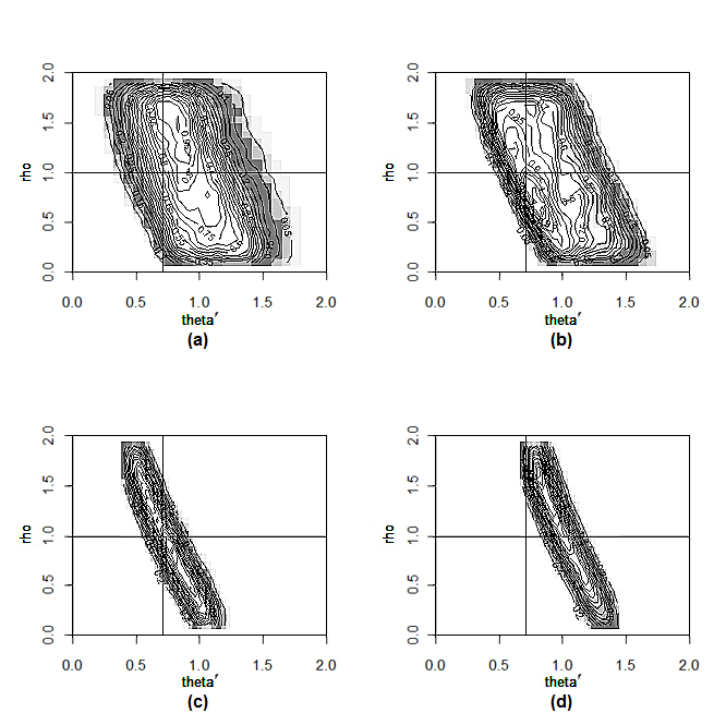
Figure 1: Inferred posterior 2D likelihood surface obtained for data with known parameters ($\theta^{\prime}=0.71$, $\tau_{1}=0.3$, $\tau_{2}=0.7$ and $\rho=1$): (a) Marginal 2D likelihood surface for ($\theta^{\prime}$, $\rho$); (b) Marginal 2D likelihood surface for ($\theta^{\prime}$, $\rho$) assuming $\tau_{1}=0.3$ (true); (c) 2D likelihood surface for ($\theta^{\prime}$, $\rho$) assuming $\tau_{1}=0.3$ (true) and $\tau_{2}=0.7$ (true); (d) 2D likelihood surface for ($\theta^{\prime}$, $\rho$) assuming $\tau_{1}=0.5$ (any value) and $\tau_{2}=1$ (any value).

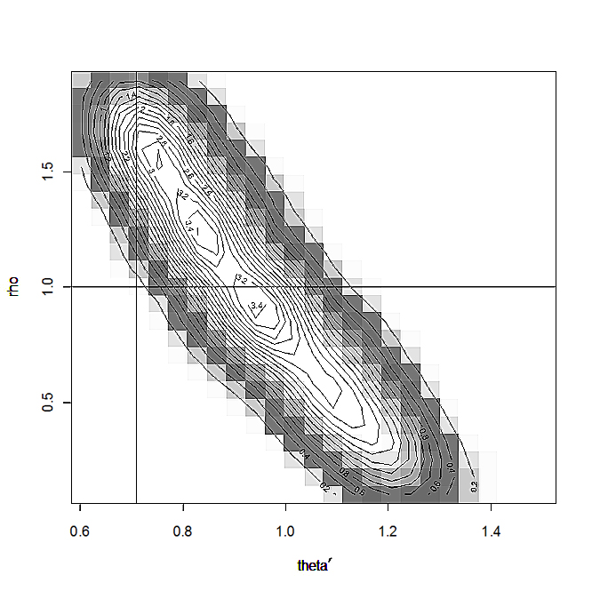
Figure 2: Inferred posterior 2D likelihood surface obtained for data with known parameters ($\theta^{\prime}=0.71$, $\tau_{1}=0.5$, $\tau_{2}=1$ and $\rho=1$): Posterior 2D likelihood surface for ($\theta^{\prime}$, $\rho$) assuming $\tau_{1}=0.5$ (true) and $\tau_{2}=1$ (true) has a shift and does not contain the true ($\theta^{\prime}$, $\rho$) at its highest probability area.

In our second example, we simulate a data set using values for the gravity parameters $\theta^{\prime}=0.71$, $\tau_{1}=0.5$, $\tau_{2}=1$ and $\rho=1$. Figure 2 is a plot of the two-dimensional likelihood in $\theta^{\prime}$ and $\rho$ space obtained by fixing $\tau_{1}$ and $\tau_{2}$ at their true values 0.5 and 1 respectively. We can see here that the true values of the parameters of interest are not in the region where the likelihood is maximized. This, unfortunately, means that repeating the above with other simulated data with different true values for the gravity parameters reveals that the ridge analogous to the ridge in Figure 1 (c) does not always have to contain the true values for $\theta^{\prime}$ and $\rho$. From our study of multiple simulated data, we also find that the likelihood ridge can have an intercept that is different from the ridge that we would intuitively think as the true ridge while having the same slope. This difference in intercepts creates a shift thereby resulting in poor parameter inference. Unfortunately the magnitude and direction of the shift depends on the true parameter values, so no simple bias correction is available. At first, one may think that the discretization of the parameters $\tau_{2}$ and $\rho$ may be causing some of these issues. We verify that this is not the case by simply computing the values of the true likelihood function at the top of the ridges obtained with the discretized likelihood. We are able to see that the likelihood surface using the discretization is similar to the true likelihood surface. The poor inference from our traditional Bayes approach is therefore clearly not a result of the discretization.

By generating additional simulations using a simpler model where we fix all the latent variables at their means we also find the full gravity model does not substantially differ from the simpler one in terms of capturing interesting biological characteristics of the underlying dynamics of the disease. In order to study the effect of this fixing on the likelihood surface, we save the true latent variables while simulating data and use them in our gridded MCMC in place of the expectations used in our gridded MCMC algorithm. The results show that using the true values of the latent variables does not change the traditional Bayes inference. This also confirms that the shifts that we observe in the traditional Bayes approach are not due to simplifying the model in gridded MCMC algorithm (see Web Appendix B for details about these assumptions), but rather due to inherent problems with the likelihood function.

We note that our main interest is to examine whether the parameter estimates result in a model fit that is capable of reproducing important characteristics of the observations. In order to study the model fit from the gridded MCMC, we simulate a data set using the full gravity model with estimated values of the parameters, where here and throughout the paper, we use modes of the corresponding posterior density functions as estimates of the parameters. These estimates for the measles data described in Section 6.1 are $(\theta^{\prime},\tau_{1},\tau_{2},\rho)=(0.71,0.5,1,1.48)$. For the simulated data set, we calculate the two 952 dimensional vectors (number of cities in the data) of summary characteristics and plot them against the summary vectors for the observed measles data (Figure 3). We can see that the simulated data do not seem to match the actual data in terms of the maximums M and the proportions of zeros P (Figure 3 (a)-(b)). In Section 5.2, we compare the model fit obtained via the gridded MCMC to the model fit we obtain via our Gaussian process-based approach described in Section 4.

We summarize below our conclusions based on the gridded MCMC approach:

1. The confidence regions for the parameters are very wide, suggesting that there may be relatively little information even with a fairly rich data set. Hence we assume that $\tau_{1}=1$, $\tau_{2}=1$ as estimated in Xia et al. (2004) and study the joint distribution of $\theta^{\prime}$ and $\rho$, which becomes well informed by the data.

2. The fitted gravity model, using the above inference about its parameters, does not capture important biological features of the data.

3. We find that the parameter estimates from the traditional Bayes approach are shifted and the direction of the shift varies as shown in Figure 2. For example, for a simulated data set using the parameters values $(\theta^{\prime},\tau_{1},\tau_{2},\rho)=(0.71,0.5,1,1)$, our attempt to infer $\rho$ assuming other parameters are known results in an estimate $\hat{\rho}=1.5$ with a confidence region that does not contain the truth .

Figure 3: Characteristics of simulated data at the parameters obtained via the traditional Bayes approach: (a) Simulated M vs M from the data; (b) Simulated P vs P from the data.

4 Gaussian processes for emulation-based inference

Since a traditional Bayes approach suffers from the above shortcomings, we develop an alternative method that is directly linked to the characteristics of the infectious disease dynamics that are of most interest to biologists. This method is based on using a Gaussian process to emulate the gravity model. A short review of Gaussian process basics is provided in Web Appendix C.

We describe a new two-stage approach for inferring the gravity parameters. In the first stage, we simulate the gravity model at several parameter settings. For each forward simulation of the model we can calculate the vector of summary statistics based on the simulated data set. This vector is high-dimensional, 952 (354) dimensions in the case of measles data for 1944-1965 (1966-1994). Since Gaussian process-based emulation for high dimensions poses serious computational challenges, we emulate the model by fitting a Gaussian process to the Euclidean distances between the summary statistics of the simulated data at the chosen parameter settings and the summary statistics for the real data. In the second stage, we perform Bayesian inference for the observations using the GP emulator from the first stage. We also allow for additional sources of uncertainty such as observational error and model-data discrepancy as described below. We note that such two-stage approaches to parameter inference in complex models has been used to reduce computational challenges and alleviate identifiability issues (cf. Liu et al., 2009; Bhat et al., 2012).

We begin with some notation. Let $Z$ denote the vector of summary statistics of interest (e.g. proportions of zeros) calculated using the observed space-time data set. Let $\Theta$ be the gravity parameters and $Y(\Theta)$ denote the vector of summary statistics obtained using a simulation from the gravity model with the parameter setting $\Theta$. Let $\Omega=(\Theta_{1},\cdots,\Theta_{p})$ be a grid on the parameter space. Our first goal is then to model $\textbf{D}=(D_{1},\cdots,D_{p})$, where $D_{i}$ is the Euclidean distance between $Y(\Theta_{i})$ and $Z$ for $i=1,\cdots,p$. This is done in the first stage of our approach where we assume,

$$\textbf{D}|\Omega,{\bf\beta_{G}},{\bf\xi_{G}}\sim N(X{\bf\beta_{G}},\Sigma({\bf\xi_{G}}))$$ (4)

Here, $\xi_{G}=(\sigma^{2}_{G},\tau^{2}_{G},\phi_{G})$ is a vector of parameters that specify the covariance matrix, and ${\bf\beta_{G}}$ is a vector of regression coefficients. The matrix $X$ is a design matrix of dimension $p\times 5$ with $i$-th row equal to $(1,\Theta_{i}^{T})$. In other words, columns of $X$ are the values the gravity parameters, $(\theta,\tau_{1},\tau_{2},\rho)$, on the selected grid and an intercept. We use Gaussian covariance matrix, $\Sigma(\xi_{G})$, elements of which are given by,

$$(\Sigma(\xi_{G}))_{ij}= \mbox{cov}(D_{i},D_{j})=$$

$$=\begin{cases}\sigma_{G}^{2}\exp(-\phi_{G}^{2}||\Theta_{i}-\Theta_{j}||^{2}),&\mbox{if }i\neq j\\ \sigma_{G}^{2}+\tau_{G}^{2},&\mbox{otherwise.}\end{cases}$$

Here, $||a-b||:=d(a-b,a-b)$, where throughout the paper, the function $d(\cdot,\cdot)$ returns the Euclidean distance between the argument vectors. Then, if we let the maximum likelihood estimate of $({\bf\beta_{G}},{\bf\xi_{G}})$ be $(\hat{\beta}_{G},\hat{\xi}_{G})$, using standard multivariate normal theory (cf. Anderson, 1984), the normal predictive distribution for the simulated distance $D$ at a new $\Theta$ can be obtained by substituting $(\hat{\beta}_{G},\hat{\xi}_{G})$ in place of $(\beta_{G},\xi_{G})$ and conditioning on D. We denote this predictive distribution by $\eta(D;\Theta)$. Detailed version of constructing this predictive distribution (emulator) is given in Web Appendix D.

Consider a new space-time data set, and let the vector of summary statistics for these data be $Y^{\ast}$. Let the distance between $Y^{\ast}$ and $Z$ be $D^{\ast}$. The predictive distribution from the first stage provides a model for $D^{\ast}$, $\eta(D^{\ast};\Theta^{\ast})$, connecting it to some unknown parameter vector $\Theta^{\ast}$.

Following Bayarri et al. (2007), we model the discrepancy between the gravity model and the real data. Failing to account for data-model discrepancy can lead to poor inference as pointed out in Bayarri et al. (2007) and Bhat et al. (2010). We account for this by setting $D^{\ast}=D^{\ast}_{\delta}:=\delta$, where $\delta>0$ is the discrepancy term. It is positive since it represents an Euclidean distance that is non-negative (in the unrealistic case that there is an exact match between the model for the data and the model used to fit the data, $\delta$ would be identically equal to 0). We then infer the gravity parameters using $\eta(D^{\ast}_{\delta};\Theta^{\ast})$ considering $\delta$ to be another unknown parameter in the MCMC algorithm. In other words, the likelihood function we use for our MCMC algorithm is a function $f(\delta,\Theta^{\ast}):=\eta(D^{\ast}_{\delta};\Theta^{\ast})$. We note that including a model discrepancy term results in more reliable parameter inference with narrower confidence regions since it adjusts for the fact that even the best model fit is not going to reduce the distance between the simulated and observed summary statistics to zero. In our simulated examples, where data are generated from the gravity model, the discrepancy term can be thought of as an adjustment parameter for the fact that two data sets simulated at the same parameter settings will always have small differences due to stochasticity. In these examples, as it is expected, estimate of the discrepancy is very small compared to the discrepancy term inferred from the original data. We also note that using negative values for $\delta$ would mean an extrapolation in our emulator beyond the grid of the parameter space that may lead to unreliable inference. In many situations, having a well-defined discrepancy term with an informative prior helps to reduce problems with identifiability of the parameters as well (cf. Craig et al., 2001).

We can now summarize our inferential approach as follows:

1. Emulating the gravity model:

   1. Select a grid $(\Theta_{1},\cdots,\Theta_{p})$ on the range of possible values for $\Theta$.

   2. Calculate $Y(\Theta_{i})$ using a simulation from the gravity model with $\Theta_{i}$ for all $i$.

   3. Calculate $\textbf{D}=(D_{1},\cdots,D_{p})$, distances from $Y_{i}$ to $Z$ for all $i$.

   4. Find the maximum likelihood estimates of $({\bf\beta_{G}},{\bf\xi_{G}})$, the parameters of the Gaussian process in Equation (4). Obtain the predictive distribution $\eta(D;\Theta)$.

2. Bayesian inference for $\delta$ and $\Theta^{\ast}$ given the observations $Z$:

   1. Using the predictive distribution with a discrepancy term, $\eta(D^{\ast}_{\delta};\Theta^{\ast})$, perform Bayesian inference for the parameters $(\Theta^{\ast},\delta)$ from the posterior distribution via MCMC.

5 Emulation-based inference for the gravity TSIR model

In this section we describe details of the application of the inferential approach described in Section 4 to the gravity TSIR model. By using simulated data examples, we show that the approach resolves the problems posed by traditional approaches. In order to contrast our approach to a traditional likelihood-based approach (carried out by gridded MCMC as described in Section 3.1), we also provide computational details from the application of both methods.

5.1 Computational details of gridded MCMC and emulation-based approaches

Inference for both the traditional Bayes and emulator-based approaches relies on sampling from the corresponding posterior distributions via MCMC. In both methods, we use univariate sequential slice sampling updates for the continuous parameters (Neal, 2003; Agarwal and Gelfand, 2005). Parameters that are on the grid are updated via an analog of a simple random walk for discrete variables. In all the MCMC algorithms that are used for the discretized MCMC approach, the chain is run until we obtain 200,000 samples. This takes about 3 days on a Intel Xeon E5472 Quad-Core 3.0 GHz processor. In all the MCMC algorithms for the Gaussian process-based method, all the updates are carried out using slice sampling since all the parameters here are continuous. Chain lengths are 200,000 again and it takes about 10 hours to generate them. The chain lengths in both methods are adequate for producing posterior estimates with small Monte Carlo standard errors (Flegal et al., 2008; Jones et al., 2006).

We emulate the gravity model with a Gaussian process using proportions of zeros as a summary statistic of interest. Our selection of proportions of zeros as the primary summary statistic of the analysis is based on suggestions by domain experts and intuition that these summary statistics are the most informative regarding the parameters of interest. It could be argued that big cities do not have bi-weeks without incidences of measles making the proportions of zeros for these cities equal to 1. However, during the course of outbreaks in these cities, the epidemic trajectory of measles is nearly unaffected by infection that may enter from neighboring locations. This means that big cities may not contain information about the gravity parameters - parameters of the movement of the infection between cities from data on number of cases of measles. In our data, more than $90\%$ of the cities may be considered as small cities. Spatial transmission is very important to the dynamics of measles for these smaller cities where the infection may become locally extinct. For small cities, infection re-entered from other cities is the only possible way to start a new outbreak.

Using different summary statistics may, of course, lead to different inference. Inference based on the maximums, however, was identical to what is obtained here and therefore we do not include details of the analysis and the corresponding results. It is also possible to develop an emulator using these two summary statistics at the same time; this is computationally more demanding and based on our exploratory data analysis will not impact our conclusions.

In general the most informative summary statistics are not trivial to judge, and depend on the disease and available data. The choice of summary statistics is closely linked to the particular inference questions addressed and can be limited by the availability of informative statistics for any particular model parameters. In cases when there are no well-established summary statistics and/or scientifically important aspects of the disease dynamics that need to be captured, our emulation-based approach can be used with summary statistics constructed/selected via algorithms borrowed from the approximate Bayesian computation literature (cf. Fearnhead and Prangle, 2012; Blum and François, 2010; Nunes and Balding, 2010; Sisson and Fan, 2010). A possible approach to the lack of informative summary statistics is to increase the number of summary statistics, thereby hoping to increase the amount of information regarding the unknown parameters (Sousa et al., 2009). This approach could, however, make our inferential methods more computationally expensive. Another method for selecting summary statistics is based on ordering summary statistics according to whether their inclusion in the analysis substantially improves the quality of inference defined by different criteria (Nunes and Balding, 2010; Joyce and Marjoram, 2008). Finally, one may construct informative summary statistics using different dimension reduction techniques (Wegmann et al., 2009; Fearnhead and Prangle, 2012; Blum and François, 2010) or by transforming the existing summary statistics (Blum, 2010).

We use the priors for the gravity model parameters that are described in Section 3. Since the discrepancy term, $\delta$, is always positive, we use an $\text{exponential}(1)$ as its prior distribution.

We use a uniform grid in the four-dimensional cube, each side of which is equal to the intervals $[0,2]$. For each parameter, we use 20 different values on each axis of the cube; this grid size permits computationally expedient inference. Our analysis of simulated data sets also shows that 20 is sufficient for accurate inference. In addition, for each point on the grid, the average distances from multiple forward simulations can be used instead of the distances calculated from a single simulation. This may be important when model realizations are highly variable. For the parameters of the gravity model, however, our inference was insensitive to the number of repetitions. This was because multiple realizations from the probability model varied very little for a given parameter setting. Therefore, it was much more important to use our computational resources for emulation across more parameter settings than it was to obtain repeated realizations at the same setting. Hence, we used one simulated time-series at each location for each set of parameters in the four-dimensional cube.

5.2 Application to simulated data

In the simulated examples that follow, our goal is to compare inference based on the GP-approach to inference from the traditional Bayes approach. In Figure 4, we show a simulated example where both the GP and traditional Bayes approaches yield the same inference, and another simulated example where the two approaches yield different answers. In both cases, the emulation-based approach provides inference that captures the true parameter values. In the first simulated data, the true parameters are $\theta^{\prime}=1$, $\tau_{1}=0.6$, $\tau_{2}=1$ and $\rho=1$. In Figure 4 (a), we overlay two different 95% confidence regions obtained using the two different methods. Both of these regions are found by assuming $\tau_{1}=0.6$ and $\tau_{2}=1$. We can see that for this example, both solid (traditional Bayes) and dashed (GP emulator-based) regions contain the true values of $\theta^{\prime}$ and $\rho$. This shows that inference based on the GP emulator is as good as inference based on the traditional Bayes method. To demonstrate that the new approach is better than the traditional Bayes approach, we choose a second set of values for the gravity parameters ($\theta^{\prime}=0.71$, $\tau_{1}=0.62$, $\tau_{2}=1$ and $\rho=1.5$) for which we know inference based on the traditional Bayes approach to be poor (like in Figure 2). Figure 4 (b) shows how the 95% confidence region from the traditional Bayes method (outlined with a solid line) is shifted and does not contain the truth. The permissible region obtained using the GP emulator (outlined with a dashed line) has corrected the shift and contains the true values of the parameters.

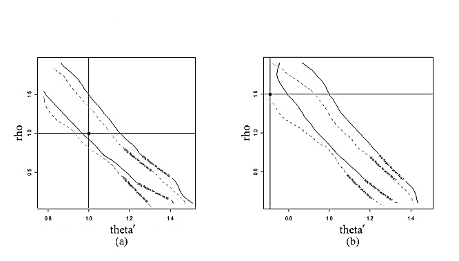
Figure 4: 95% C.I.’s for ($\theta^{\prime}$, $\rho$) obtained via different methods (assuming that $\tau_{1}$ and $\tau_{2}$ are known): Solid line shows the 95% region obtained using the traditional Bayes method. Dashed line outlines the 95% region obtained via GP emulator: (a) Both regions contain the true parameter values; (b) Region obtained by the GP emulator contains the true values of the parameters, while the traditional Bayes region does not.

We analyze the ability of the fitted gravity model to reproduce the key characteristics of the process at these new parameter estimates. Using estimates obtained via the GP-emulator based approach, $(\theta^{\prime},\tau_{1},\tau_{2},\rho)=(0.71,0.5,0.5,1.48)$, we generate a data set to obtain plots similar to the ones in Figure 3. Plots on Figure 5 (a)-(b) show that the model now can fit the maximums M and the proportions of zeros P very well. Comparing the plots in Figures 3 and 5, we can now say that the new emulation-based approach improves the model fit substantially while the traditional Bayes parameter estimates from the gridded MCMC fail to provide a model that captures the key epidemiological features of the data.

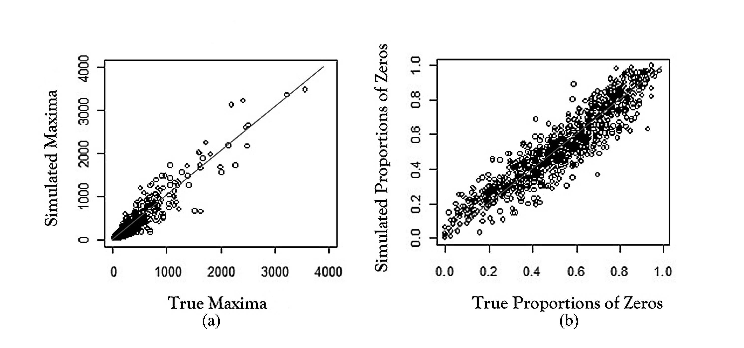
Figure 5: Characteristics of simulated data at the parameters chosen to minimize the discrepancy between the data and the simulation: (a) Simulated M vs M from the data; (b ) Simulated P vs P from the data.

In order to study the effect of a discrepancy term in our approach, we also tried to infer the gravity parameters using the emulation-based model with $\delta=0$ (no discrepancy). The resultant 95% confidence regions were much wider for the latter approach containing incorrect parameter settings, supporting the points made in Bayarri et al. (2007) about the importance of adding a discrepancy term to approximate models. We note, however, that these new confidence regions still contained the true parameters values in simulated examples and did not have the kinds of shifts seen in parameter inference using grid-based MCMC as in Section 3.1. This means that the problem when the true parameters of the model are not recovered by a likelihood-based approach is not related to the issue of accounting for model-data discrepancy.

Continuing to explore the effect of the discrepancy term, we also tried a few different priors for $\delta$; using the exponential(1) prior for the discrepancy term worked very well as was clear from the results. The posterior median for the discrepancy term was found to be around $2$ which was close to the minimal distance from the simulated and the true vectors of summary statistics taken over all the points on the grid.

6 Results from application to measles data

We apply our emulation-based approach to inference for the gravity TSIR model to a well known measles data set from the U.K. The purpose of this is twofold: to demonstrate the applicability of our approach to a real data set as well as to provide some insights into measles dynamics in the pre-vaccination era.

6.1 Description of measles data set

The following description of the data closely follows Xia et al. (2004). We analyze weekly case reports of measles for cities in England and Wales. The data is available for K = 952 locations in the pre-vaccination era from 1944 to 1965 and for K = 354 locations from 1966 to 1994 with information on vaccine coverage. The data represent an interesting case study of spatiotemporal epidemic dynamics (Grenfell et al., 2002) with well understood underreporting rate of 40$\%$-55$\%$ (Bjørnstad et al., 2002). Besides the under-reporting, the data are complete and reveal inter-annual outbreaks of infection. A critical feature of this data set is that, except for a few large cities, infection frequently goes locally extinct, so that overall persistence hinges on episodic reintroduction and spatial coupling. Before further analysis, we correct the reported data by a factor of 1/0.52, with 52% being the average reporting rate taken from previous analysis (Bjørnstad et al., 2002; Clarkson and Fine, 1985; Finkenstädt and Grenfell, 2000). In addition, as in previous works, we use a timescale that represent the exposed and infectious period, which is known to be about 2 weeks for measles (Black, 1989).

In the analysis of the data for pre-vaccination era, following a standard assumption in the literature (see, for instance, Xia et al., 2004; Bjørnstad et al., 2002; Grenfell et al., 2002, and the references therein), the population sizes and per capita birth rates for all locations in this work are assumed to be approximately constant throughout the time period. These variables are taken as those in 1960 for each of the areas. This is a rough approximation, since most communities grew during the period we analyze. The force of infection is, therefore, on average slightly underestimated (overestimated) during the early (late) part of the study. In the analysis of the newer data for 1966-1994, the population sizes and per capita birth rates are allowed to be variable as specified in the gravity model. We note that these assumptions are made for the consistency of our work with the previous analysis and do not have an effect on our inference and/or conclusions.

6.2 Some implications for measles dynamics

Important biological questions we want to answer based on these data are: (i) do the gravity model parameters (and hence disease transmission) change for school holiday periods versus non-holiday periods? Do they change for different time periods (before and after vaccines against measles were available)? (ii) do movement rates of infected people change in different time periods?

In order to answer these questions, using our emulator-based approach, we first fit the model to the parts of the data corresponding to periods of holidays and non-holidays. As demonstrated in our simulated examples in Section 3.1 and 5.2, it is not possible to infer all the gravity model parameters at once. Hence, we set the parameters $\tau_{1}$ and $\tau_{2}$ equal to 1 and study the remaining key gravity model parameters $\theta$ and $\rho$. The resulting 95% confidence regions for $\theta^{\prime}$ and $\rho$ are provided in Figure 6 (a). As can be seen from this figure, the two regions are almost identical, indicating that any change in the number of cases of measles for holidays and non-holidays is not due to the change in the way the infection spreads between cities of the metapopulation during these periods.

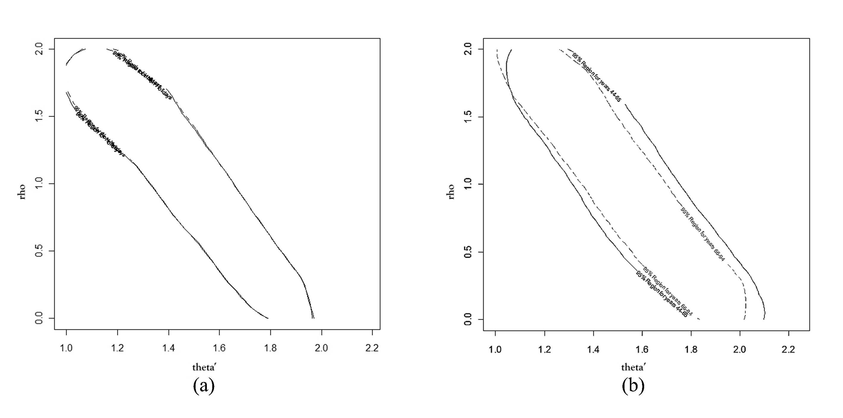
Figure 6: 95% C.I. for ($\theta^{\prime}$, $\rho$) obtained via fitting GP emulator to a part of the data: (a) Solid line outlines the confidence region for parameters when data from only holiday periods are used; Dashed line outlines the confidence region for parameters when data for only non-holiday periods are used; (b) Solid line outlines the confidence region for parameters when data for years from 1944 -1965 are used; Dashed line outlines the confidence region for parameters when data for years from 1966 - 1994 are used.

Since the matrix $M=\{m_{kj}\}$, where $m_{kj}=\theta^{\prime}N_{kt}^{\tau_{1}}\sum\limits_{t=1}^{T}\frac{(I{jt})^{\tau_{2}}}{d_{kj}^{\rho}}$ is interpreted as a matrix of the amount of movement, sum of $k$-th row of $M$ represents the amount of infected individuals leaving city $k$ while sum of $k$-th column is the number of infected people coming to city $k$. Using samples for $\theta^{\prime}$ and $\rho$, we easily obtain a sample for the spatial flux of infection for selected cities. In Table 1, we report our estimates with corresponding credible regions based on this analysis. We use the posterior median as point estimates. For example, we estimate the average number of emigrating infections during the holiday periods each week to be equal to 31.1 for London. Below the estimate, we report a 95% credible interval for it which is (4.4, 479.1). Based on these estimates, the mobility of the infection appears to be less during the periods of holidays.

Table 1: Estimated amount of average movement in two weeks

City	From		To
	Holiday	Non-Holiday	Holiday	Non-Holiday
London	31.1	46.6	34.4	49.8
	(4.4, 479.1)	(6.6, 744.7)	(4.6, 564.9)	(6.9, 823.9)
Birmingham	7.5	10.8	7.5	11.5
	(1.2, 72.9)	(1.8, 110.6)	(1.2, 74.7)	(1.9, 115.8)
Manchester	7.8	10.3	9.1	10.8
	(1.0, 151.4)	(1.4, 180.9)	(1.2, 162.9)	(1.5, 189.1)
Blackpool	0.8	1.1	0.6	0.7
	(0.1, 6.7)	(0.2, 8.8)	(0.1, 5.2)	(0.1, 6.1)

Figure 6 (b) shows confidence regions obtained by the GP emulator-based approach by fitting the model to the data from 1944-1965 and 1966-1994 separately. From this figure, we conclude that the change in parameter values is statistically insignificant for these two different time periods. The important scientific implication of this result is that introduction of vaccination in England and Wales in 1966 does not change the movement patterns of the infection between cities. This also means that any observed change in incidence rates of measles is only due to the effects of vaccination, not a change in movement patterns in the vaccination era. Table 2 shows estimates of the average amount of transit infections each bi-week for years 1944-1965 and 1966-1994. We see here that the infection appears to move less during the later years. We note that none of the differences are statistically significant. As a visual summary of this table for the time period with vaccination, in Figure 7, we plot histograms of log-transformed estimated amount of average movement in two weeks for 1966-1994. From these plots, we can conclude that both incoming (Figure 7 (a)) and outgoing (Figure 7 (b)) number of infections for most of the cities is very small.

Table 2: Estimated amount of average movement in two weeks

City	From		To
	1944-65	1966-1994	1944-65	1966-1994
London	48.1	39.2	51.6	42.4
	(7.9, 488.4)	(4.4, 623.2)	(7.0, 591.5)	(4.9, 739.8)
Birmingham	12.9	9.3	13.5	9.1
	(1.9, 75.1)	(1.2, 112.8)	(2.8, 93.7)	(1.2, 121.3)
Manchester	12.4	10.1	14.0	10.1
	(2.1, 128.4)	(0.9, 176.7)	(1.9, 163.6)	(1.4, 193.1)
Blackpool	1.1	0.9	0.9	0.8
	( 0.3, 8.1)	(0.2, 9.7)	(0.1, 7.4)	( 0.1, 7.1)

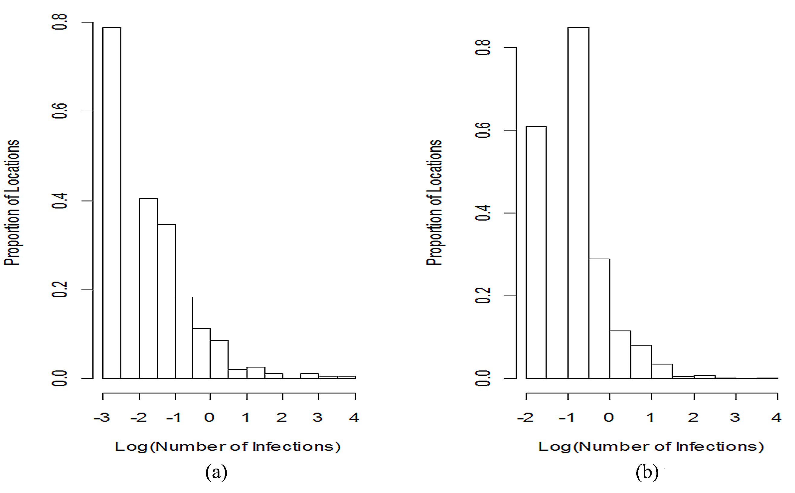
Figure 7: Histogram of estimated amount of average movement in two weeks for 1966-1994: (a) outgoing infections; (b) incoming infections.

Figure 8 displays graphs of networks of the movement of measles between cities in our data. These graphs are obtained using the movement matrix $M$ and estimates of the gravity parameters from data for 1966-1994 via the GP emulator-based approach. In Figure 8 (a), we plot the network of outgoing infections. In Figure 8 (b) we plot the network of incoming infections for cities of the metapopulation. Figure 8 (a) illustrates the importance of big cities in the dynamics of measles for smaller communities where the infection may become locally extinct. From this figure, we see that the edges radiating from the populated cities reach the small cities causing a re-introduction of the infection in these communities. This link between big and small cities do not seem to depend on distances between the cities. On the other hand, in Figure 8 (b), we see that the amount of incoming infections is mostly dependent on distances between cities since edges connecting different cities in this graph are shorter relative to the edges of the graph in Figure 8 (a). This means that big cities are the only important factors in starting an outbreak in smaller cities, excluding the possibility of re-introduction of the disease from neighboring cities with small population sizes.

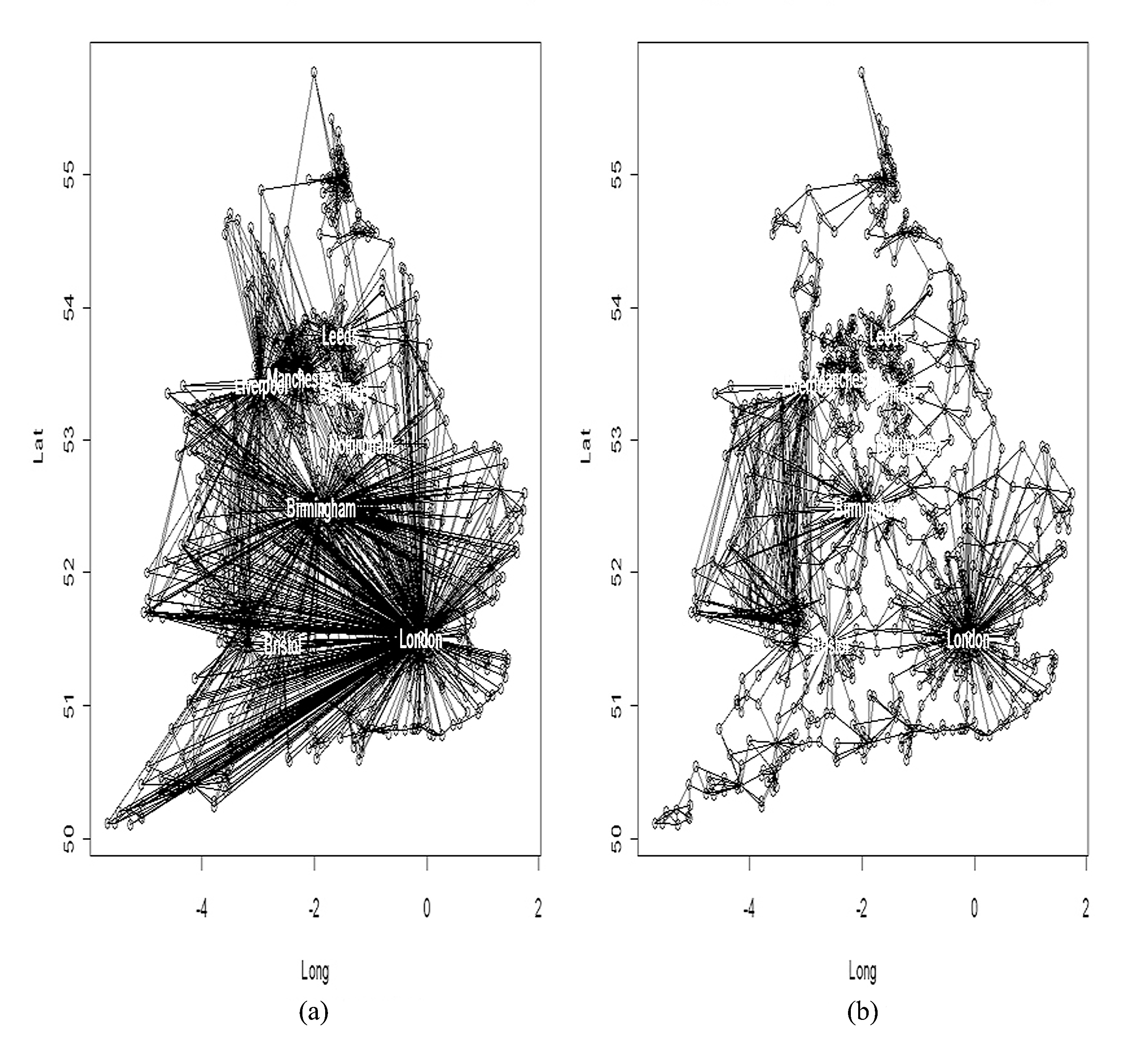
Figure 8: Movement networks of the infection: (a) network of outgoing infections; (b) network of incoming infections.

7 Discussion

Complex models are very useful for representing physical phenomena, whether the phenomena is the spread of an infectious disease or the change in sea surface temperatures in the Atlantic. As is well known, it is not always possible for every aspect of such complicated phenomena to be modeled accurately; certain key characteristics of the process necessarily have to be focal points of the modeling effort. However, these key characteristics are not typically the focus of a statistical inferential procedure that uses a traditional likelihood-based approach. The approach we have developed in this paper addresses this point by providing a flexible inferential method that directly takes into account the characteristics of the process that are most important to scientists. Even though focusing on different summary statistics can lead to different estimates, parameter inference based on our approach produces an improved model fit to the biologically interesting features of the infectious disease dynamics. In addition to the flexibility this provides, we find that our approach is also computationally tractable in situations where traditional likelihood-based inference is not. In general, when there are no obvious summary statistics and/or scientifically important aspects of the disease dynamics that need to be captured and informative for parameter inference, as was mentioned in Section 5, one can employ our approach with summary statistics constructed or selected via existing algorithms in the approximate Bayesian computation literature (cf. Fearnhead and Prangle, 2012; Blum and François, 2010; Nunes and Balding, 2010; Joyce and Marjoram, 2008; Wegmann et al., 2009; Blum, 2010; Sisson and Fan, 2010).

Computer model emulation and calibration is an active area of research (cf. Kennedy and O’Hagan, 2001; Bayarri et al., 2007; Sansó and Forest, 2009; Rougier and Beven, 2009; Rougier et al., 2009; Conti and O’Hagan, 2010; Bhattacharya, 2007; Higdon et al., 2008; Bhat et al., 2010) but most of this work has focused on deterministic models.

Some authors have also worked on applying the ideas from computer model emulation and calibration literature in the context stochastic nonlinear ecological dynamical systems and complex models is biology (cf. Wood, 2010; Henderson et al., 2009). The main idea in these papers is to assume the selected summary statistics are normally distributed random variables with unknown mean and variance functions that depend on the parameters of interest of the original model. In the emulation step, these functions are then estimated from data by utilizing two different inference algorithms (details are available in Henderson et al. (2009) and Wood (2010)). In contrast to their approaches, we emulate the scientifically important summary statistics directly. That is, we model the summary statistics, in our case the proportion of zeroes at each of 952 (or 354) different cities, depending on the data set. This results in a 952-dimensional summary statistic corresponding to the observations as well as a 952-dimensional summary statistic for each simulated data set. While the other approaches may be easier to implement in cases where the summary statistics may be assumed to be normally distributed, for the kind of problem we are considering, our Gaussian process model provides a much more flexible model for the multivariate summary statistics. In the other approaches, a normal model is assumed for the summary statistics and the Gaussian process model is used to obtain a flexible model for the means and variances as a function of the parameters; in fact, this is why their approaches often utilize transformations of the summary statistics in order to make the assumption of normality more reasonable. In our approach, a Gaussian process model (a flexible infinite-dimensional process) is used to model the summary statistics directly as a function of the parameters. Hence, our emulation approach captures well potentially complicated relationships between the parameter and the multivariate summary statistics, while also providing uncertainties about this relationship; the uncertainties in the other approaches describe uncertainties about the mean and variances of an assumed normal distribution model for the summary statistics.

Additionally, in our approach we account for the fact that there is a discrepancy between the output of the biological model and the data. That is, we do not assume that the biological model captures the true process perfectly even at some ideal parameter setting. We allow for an additional process that accounts for data-model discrepancies. This is important for obtaining reasonable parameter inference as also pointed out in Bayarri et al. (2007) and Bhat et al. (2012). In our view, therefore, our paper makes the following main contributions: (1) a general inferential approach that focuses on characteristics (summary statistics) of a process; (2) a method for statistical inference when the likelihood is intractable and simulation from the probability model is expensive; (3) a study of a particular model for measles dynamics, the gravity TSIR model, using the approach we have developed.

In the context of measles in the pre-vaccination and vaccination eras, our method allows us to study some interesting aspects of the dynamics of measles based on the gravity TSIR model. For instance, we find that there does not appear to be a significant change in the gravity parameters for the school holiday periods versus non-holidays which means that we do not have enough evidence of a change in the dynamics of measles between these different periods. By fitting the model using our approach to the data from 1944-1965 and 1966-1994 separately, we reveal that that introduction of vaccination in England and Wales in 1966 does not change the movement patterns of the infection between cities. This indicates that any observed change in incidence rates of measles is only due to the effects of vaccination. Analyzing graphs of the networks of movement of the infection obtained using the estimates of the gravity parameters from data for 1966-1994, we identify the important hubs and their roles in transmission of measles between the cities of the metapopulation. These hubs, the biggest cities, seem to spread the infection to smaller cities regardless of the distances between cities, while movement of the infection between small cities is dependent on the distances.

More generally, the methodology we have described in this paper is particularly useful in cases where simulation from a probability model might be too expensive to allow the use of other popular inferential approaches like ABC. It is worth noting that our approach works well when the parameter dimensionality is small, but is generally infeasible for parameter dimensions greater than around five to eight depending on the model complexity. Our approach is widely applicable for inference in computationally expensive but biologically realistic models. In principle, whenever a likelihood is expensive to evaluate or when traditional Bayes approaches does not capture the most scientifically relevant features of the model, our method provides a way to incorporate important characteristics in a computationally tractable inferential approach.

References

- Agarwal and Gelfand (2005) Agarwal, D. and A. Gelfand (2005). Slice sampling for simulation based fitting of spatial data models. Statistics and Computing 15(1), 61–69.
- Anderson (1984) Anderson, T. W. (1984). An Introduction to Multivariate Statistical Analysis. John Wiley & Sons.
- Bartlett (1956) Bartlett, M. S. (1956). Deterministic and stochastic models for recurrent epidemics. In J. Neyman (Ed.), Proceedings of the Third Berkeley Symposium on Mathematical Statistics and Probability, Volume 4, pp. 81–109. University of California Press.
- Bayarri et al. (2007) Bayarri, M., J. Berger, J. Cafeo, G. Garcia-Donato, F. Liu, J. Palomo, R. Parthasarathy, R. Paulo, J. Sacks, and D. Walsh (2007). Computer model validation with functional output. Annals of Statistics 35(5), 1874–1906.
- Bayarri et al. (2007) Bayarri, M., J. Berger, R. Paulo, J. Sacks, J. Cafeo, J. Cavendish, C. Lin, and J. Tu (2007). A framework for validation of computer models. Technometrics 49(2), 138–154.
- Beaumont et al. (2002) Beaumont, M., W. Zhang, and D. Balding (2002). Approximate bayesian computation in population genetics. Genetics 162(4), 2025.
- Bhat et al. (2012) Bhat, K., M. Haran, R. Olson, and K. Keller (2012). Inferring likelihoods and climate system characteristics from climate models and multiple tracers. Environmetrics 23(4), 345–362.
- Bhat et al. (2010) Bhat, K. s., M. Haran, and M. Goes (2010). Computer model calibration with multivariate spatial output. In M.-H. Chen, D. K. Dey, P. Müller, D. Sun, and K. Ye (Eds.), Frontiers of Statistical Decision Making and Bayesian Analysis: In Honor of James O. Berger, pp. 168–184. Springer-Verlag Inc.
- Bhattacharya (2007) Bhattacharya, S. (2007). A simulation approach to Bayesian emulation of complex dynamic computer models. Bayesian Analysis 2(4), 783–816.
- Bjørnstad et al. (2002) Bjørnstad, O., B. Finkenstädt, and B. Grenfell (2002). Dynamics of measles epidemics: estimating scaling of transmission rates using a time series SIR model. Ecological Monographs 72(2), 169–184.
- Black (1989) Black, F. (1989). Measles. Viral infections of humans: epidemiology and control. New York: Plenum publishingEvans AS 3, 451–65.
- Blum (2010) Blum, M. (2010). Approximate bayesian computation: a nonparametric perspective. Journal of the American Statistical Association 105(491), 1178–1187.
- Blum and François (2010) Blum, M. and O. François (2010). Non-linear regression models for approximate bayesian computation. Statistics and Computing 20(1), 63–73.
- Clarkson and Fine (1985) Clarkson, J. A. and P. M. Fine (1985). The efficiency of measles and pertussis notification in England and Wales. International Journal of Epidemiology 14(1), 153.
- Cliff et al. (1993) Cliff, A., P. Haggett, and M. Smallman-Raynor (1993). Measles: an historical geography of a major human viral disease from global expansion to local retreat, 1840-1990. Blackwell, Oxford [England]; Cambridge, Mass., USA.
- Conti and O’Hagan (2010) Conti, S. and A. O’Hagan (2010). Bayesian emulation of complex multi-output and dynamic computer models. Journal of Statistical Planning and Inference 140(3), 640–651.
- Craig et al. (2001) Craig, P., M. Goldstein, J. Rougier, and A. Seheult (2001). Bayesian forecasting for complex systems using computer simulators. Journal of the American Statistical Association 96(454), 717–729.
- Dietz (1976) Dietz, K. (1976). The incidence of infectious diseases under the influence of seasonal fluctuations. Lecture Notes in Biomathematics 11, 1–15.
- Earn et al. (1998) Earn, D., P. Rohani, and B. Grenfell (1998). Persistence, chaos and synchrony in ecology and epidemiology. Proceedings of the Royal Society B: Biological Sciences 265(1390), 7.
- Fearnhead and Prangle (2012) Fearnhead, P. and D. Prangle (2012). Constructing summary statistics for approximate bayesian computation: semi-automatic approximate bayesian computation. Journal of the Royal Statistical Society: Series B (Statistical Methodology) 74(3), 419–474.
- Fine and Clarkson (1982) Fine, P. and J. Clarkson (1982). Measles in England and Wales: an analysis of factors underlying seasonal patterns. International Journal of Epidemiology 11(1), 5.
- Finkenstädt et al. (2002) Finkenstädt, B., O. Bjørnstad, and B. Grenfell (2002). A stochastic model for extinction and recurrence of epidemics: estimation and inference for measles outbreaks. Biostatistics 3(4), 493–510.
- Finkenstädt and Grenfell (2000) Finkenstädt, B. and B. Grenfell (2000). Time series modelling of childhood diseases: a dynamical systems approach. Journal of the Royal Statistical Society: Series C (Applied Statistics) 49(2), 187–205.
- Finkenstädt et al. (1998) Finkenstädt, B., M. Keeling, and B. Grenfell (1998). Patterns of density dependence in measles dynamics. Proceedings of the Royal Society B: Biological Sciences 265(1398), 753.
- Flegal et al. (2008) Flegal, J., M. Haran, and G. Jones (2008). Markov chain Monte Carlo: can we trust the third significant figure. Statistical Science 23(2), 250–260.
- Glass et al. (2003) Glass, K., Y. Xia, and B. Grenfell (2003). Interpreting time-series analyses for continuous-time biological models–measles as a case study. Journal of theoretical biology 223(1), 19–25.
- Grenfell et al. (2002) Grenfell, B., O. Bjørnstad, and B. Finkenstädt (2002). Dynamics of measles epidemics: scaling noise, determinism, and predictability with the TSIR model. Ecological Monographs 72(2), 185–202.
- Grenfell et al. (2001) Grenfell, B., O. Bjornstad, and J. Kappey (2001). Travelling waves and spatial hierarchies in measles epidemics. Nature 414(6865), 716–723.
- Grenfell and Harwood (1997) Grenfell, B. and J. Harwood (1997). (Meta) population dynamics of infectious diseases. Trends in Ecology & Evolution 12(10), 395–399.
- Henderson et al. (2009) Henderson, D., J. Richard, K. Krishnan, C. Lawless, and D. Wilkinson (2009). Bayesian emulation and calibration of a stochastic computer model of mitochondrial dna deletions in substantia nigra neurons. Journal of the American Statistical Association 104(485), 76–87.
- Higdon et al. (2008) Higdon, D., J. Gattiker, B. Williams, and M. Rightley (2008). Computer model calibration using high-dimensional output. Journal of the American Statistical Association 103(482), 570–583.
- Jones et al. (2006) Jones, G., M. Haran, B. Caffo, and R. Neath (2006). Fixed-width output analysis for Markov chain Monte Carlo. Journal of the American Statistical Association 101(476), 1537–1547.
- Joyce and Marjoram (2008) Joyce, P. and P. Marjoram (2008). Approximately sufficient statistics and bayesian computation. Statistical Applications in Genetics and Molecular Biology 7(1), 1–16.
- Keeling et al. (2004) Keeling, M. J., O. N. Bjørnstad, and B. T. Grenfell (2004). Metapopulation dynamics of infectious diseases., pp. 415–445. Elsevier.
- Kennedy and O’Hagan (2001) Kennedy, M. and A. O’Hagan (2001). Bayesian calibration of computer models. Journal of the Royal Statistical Society: Series B (Statistical Methodology) 63(3), 425–464.
- Liu et al. (2009) Liu, F., M. Bayarri, and J. Berger (2009). Modularization in Bayesian analysis, with emphasis on analysis of computer models. Bayesian Analysis 4(1), 119–150.
- Marjoram et al. (2003) Marjoram, P., J. Molitor, V. Plagnol, and S. Tavaré (2003). Markov chain Monte Carlo without likelihoods. Proceedings of the National Academy of Sciences of the United States of America 100(26), 15324.
- McLean and Anderson (1988) McLean, A. and R. Anderson (1988). Measles in developing countries Part I. Epidemiological parameters and patterns. Epidemiology and infection 100(01), 111–133.
- Neal (2003) Neal, R. (2003). Slice sampling. Annals of Statistics 31(3), 705–741.
- Nunes and Balding (2010) Nunes, M. and D. Balding (2010). On optimal selection of summary statistics for approximate bayesian computation. Statistical applications in genetics and molecular biology 9(1).
- Pritchard et al. (1999) Pritchard, J., M. Seielstad, A. Perez-Lezaun, and M. Feldman (1999). Population growth of human Y chromosomes: a study of Y chromosome microsatellites. Molecular Biology and Evolution 16(12), 1791.
- Rougier and Beven (2009) Rougier, J. and K. Beven (2009). Formal bayes methods for model calibration with uncertainty. Applied Uncertainty Analysis for Flood Risk Management, eds. Beven, K. and Hall, J., Imperial College Press/World Scientific.
- Rougier et al. (2009) Rougier, J., S. Guillas, A. Maute, and A. D. Richmond (2009). Expert knowledge and multivariate emulation: the thermosphere ionosphere electrodynamics general circulation model (TIE-GCM). Technometrics 51(4), 414–424.
- Sacks et al. (1989) Sacks, J., W. Welch, T. Mitchell, and H. Wynn (1989). Design and analysis of computer experiments. Statistical science 4(4), 409–423.
- Sansó and Forest (2009) Sansó, B. and C. Forest (2009). Statistical calibration of climate system properties. Journal of the Royal Statistical Society: Series C (Applied Statistics) 58(4), 485–503.
- Sisson and Fan (2010) Sisson, S. and Y. Fan (2010). Likelihood-free markov chain monte carlo. arXiv preprint arXiv:1001.2058.
- Sousa et al. (2009) Sousa, V., M. Fritz, M. Beaumont, and L. Chikhi (2009). Approximate bayesian computation without summary statistics: the case of admixture. Genetics 181(4), 1507–1519.
- Swinton and Grenfell (1998) Swinton, H. and G. Grenfell (1998). Persistence thresholds for phocine distemper virus infection in harbour seal Phoca vitulina metapopulations. Journal of Animal Ecology 67(1), 54–68.
- Wegmann et al. (2009) Wegmann, D., C. Leuenberger, and L. Excoffier (2009). Efficient approximate bayesian computation coupled with markov chain monte carlo without likelihood. Genetics 182(4), 1207–1218.
- Wood (2010) Wood, S. (2010). Statistical inference for noisy nonlinear ecological dynamic systems. Nature 466(7310), 1102–1104.
- Xia et al. (2004) Xia, Y., O. Bjørnstad, and B. Grenfell (2004). Measles metapopulation dynamics: a gravity model for epidemiological coupling and dynamics. American Naturalist 164(2), 267–281.