Beyond the fibre: Resolved properties of SDSS galaxies

Abstract

We have used the VIMOS integral field spectrograph to map the emission line properties in a sample of 24 star forming galaxies selected from the SDSS database. In this data paper we present and describe the sample, and explore some basic properties of SDSS galaxies with resolved emission line fields. We fit the H$\alpha$+[NII] emission lines in each spectrum to derive maps of continuum, H$\alpha$ flux, velocity and velocity dispersion. The H$\alpha$, H$\beta$, [NII] and [OIII] emission lines are also fit in summed spectra for circular annuli of increasing radius. A simple mass model is used to estimate dynamical mass within 10 kpc, which compared to estimates of stellar mass shows that between 10 and 100% of total mass is in stars. We present plots showing the radial behaviour of EW[H$\alpha$], u-i colour and emission line ratios. Although EW[H$\alpha$] and u-i colour trace current or recent star formation, the radial profiles are often quite different. Whilst line ratios do vary with annular radius, radial gradients in galaxies with central line ratios typical of AGN or LINERS are mild, with a hard component of ionization required out to large radii. We use our VIMOS maps to quantify the fraction of H$\alpha$ emission contained within the SDSS fibre, taking the ratio of total H$\alpha$ flux to that of a simulated SDSS fibre. A comparison of the flux ratios to colour-based SDSS extrapolations shows a 175% dispersion in the ratio of estimated to actual corrections in normal star forming galaxies, with larger errors in galaxies containing AGN. We find a strong correlation between indicators of nuclear activity: galaxies with AGN-like line ratios and/or radio emission frequently show enhanced dispersion peaks in their cores, requiring non-thermal sources of heating. Altogether, about half of the galaxies in our sample show no evidence for nuclear activity or non-thermal heating. The fully reduced data cubes and the maps with the line fits results are available as FITS files from the authors.

1 Introduction

The unprecedented large number of galaxies observed in the Sloan Digital Sky Survey (SDSS, York et al. 2000) has made a significant impact on our quantitative and qualitative understanding of galaxy formation and evolution. The relationships between the derived physical parameters from the SDSS galaxies, such as the star formation rates and metallicities, describe how efficiently galaxies turn their gas into stars and help constrain theoretical modelling of star formation and galaxy evolution. Unfortunately, as SDSS spectra are fibre-based, these astrophysical parameters are centrally averaged quantities only (Kewley et al. 2001, 2005; Brinchmann et al. 2004 (hereon B04); Wilman et al. 2005).

To avoid characterization of the global galaxy properties based on extrapolated central measurements requires spatially resolved observations. Integral Field Spectroscopy (IFS) is an excellent tool to map the internal structure of galaxies and to further our knowledge of these systems in the local Universe. Surveys of nearby galaxies with IFS include SAURON (Bacon et al. 2001) to study early type galaxies, PINGS (Rosales-Ortega et al. 2010) to map the properties of disk galaxies and CALIFA (Sánchez et al. 2011) an ambitious IFS survey of some 600 galaxies spanning all Hubble types in the local Universe.

A related project, GHASP (Garrido et al. 2002; Epinat et al. 2010), maps the H$\alpha$ velocities in spiral galaxies using the scanning Fabry-Perot technique in a sample of 153 nearby spiral galaxies and build up a local reference sample for comparison with high-z observations.

The SDSS database is the largest source of extra-galactic properties, albeit centrally averaged quantities only. It has a fairly uniform coverage of galaxies in the redshift range out 0.1. However, most IFS surveys cover a much more local volume, e.g. CALIFA goes out to $z<0.03$. In this paper we present an IFS study to map the properties in a sample of 24 galaxies selected from the SDSS database. These systems have EW[H$\alpha$]$>20$Å and are uniformly distributed over the redshift range 0 to 0.1. This allows us to systematically compare the centrally averaged values to the integrated properties, address aperture bias in star forming galaxies, and characterize the large scale structure of these systems in detail.

The layout of this paper is as follows. In section 2 we describe the criteria used to construct our sample of 24 SDSS galaxies. In section 3 we describe the data reduction process and the emission line analysis. We present the radial gradients and 2D maps of H$\alpha$ derived from these data and interpret them in section 4 and 5 respectively.

2 Sample

Targets were selected from the SDSS Data Release 4 (DR4). The only criteria for selection were EW[H$\alpha$]$\geq 20$Å; model r-band magnitude, $r\leq 17$; avoidance of objects with sizes much smaller or larger than the FOV (27″$\times$27″, but this covers a range of physical size at variable redshift) and suitable right ascension and declination for observation. We selected a total of 24 galaxies. For visual reference purposes we present a mosaic of the SDSS colour images in Fig. 1.

As demonstrated in the top left panel of Fig. 2, the primary selection criterion of EW[H$\alpha$]$\geq 20$Å selects some of the more strongly H$\alpha$ emitting galaxies. This corresponds to the upper $20\%$ of all galaxies in EW[H$\alpha$]. The peak at EW[H$\alpha$]$\sim 0$Å can be fit using a Gaussian whose width should represent the typical error on this measurement for a passive galaxy. Subtracting this population leaves only star-forming galaxies, of which our EW[H$\alpha$]$\geq 20$Å criterion selects the upper $27\%$.

It is also important to note that this selection is applied in terms of the fibre or central EW[H$\alpha$], and so it is possible that we miss objects with most of the line flux in the outer regions, such as face-on spiral galaxies with a passive bulge and highly star forming outer disk.

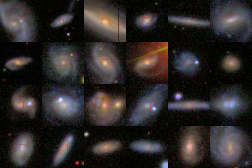
Figure 1: Colour SDSS imaging of our selected galaxies. Top to bottom, left to right, galaxies 01-06, 07-12, 13-18, 19-24. Red squares show the location of SDSS spectral fibres.

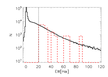
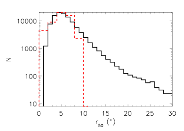
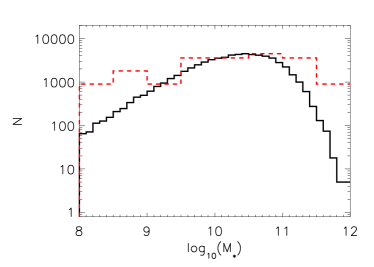
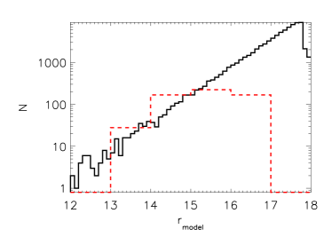
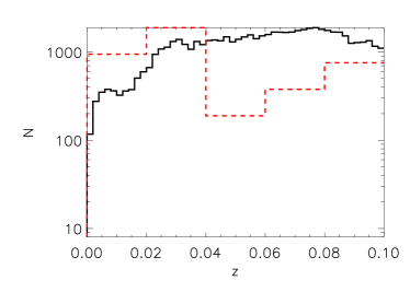
Figure 2: Top left: Distribution of EW[H$\alpha$] (B04, fibre measurements) for all SDSS DR4 galaxies (black, solid histogram) and our VIMOS targets (red, dashed histogram, scaled). By selection, we are sampling the more highly star forming galaxies (EW[H$\alpha$]$=20$Å, dotted vertical line). Top right: Distribution of $r_{50}$, the r-band Petrosian half-light radius in arcseconds. The solid black histogram represents all galaxies with EW[H$\alpha$]$\geq 20$Å, whilst our targets are represented by the dashed red histogram (renormalized). Likewise, the middle and bottom panels illustrate the derived stellar mass (Gallazzi, 2006), r-band model magnitude and redshift distributions of the EW[H$\alpha$]$\geq 20$Å population and our targets respectively.

The other four panels of figure 2 show how our targets (red, dashed histograms) are distributed in the radius containing 50% of the Petrosian r-band flux ($r^{{}^{\prime\prime}}_{50}$), stellar mass ($M_{*}$, Gallazzi et al, 2006), r-band model magnitude and redshift compared to the overall SDSS DR4 distribution of EW[H$\alpha$]$\geq 20$Å objects (black, solid histograms). We cover this parameter space, excluding only the galaxies with large apparent sizes ($r_{50}>10\arcsec$) for which we would not have been able to observe close to the whole galaxy in one VIMOS pointing.

Table 1: Properties of the galaxies in our VIMOS IFU sample derived from SDSS DR5. Listed in column six are luminosity distances. The SDSS derived $r$-band model magnitude and Petrosian radius are listed in columns eight and nine respectively.

Name	SDSS name	RA	Dec	$z$	$D_{L}^{1)}$	scale	$r_{\rm model}$	$r_{P}$	EW[H$\alpha$]
		(J2000)	(J2000)		Mpc	kpc/$\prime\prime$		(arcsec)
gal01	SDSS J081753+002235	08h17m53s	+03d22m35s	0.030	129.7	0.593	15.52	16.43	20.08
gal02	SDSS J085555+034530	08h55m55s	+03d45m30s	0.028	120.8	0.554	15.50	10.43	34.33
gal03	SDSS J091750$-$001642	09h17m50s	$-$00d16m42s	0.017	72.7	0.341	13.87	20.69	21.72
gal04	SDSS J091844+073713	09h18m44s	+07d37m13s	0.106	484.1	1.919	16.16	5.88	30.05
gal05	SDSS J092001+070322	09h20m01s	+07d03m22s	0.012	51.2	0.242	16.17	14.06	29.26
gal06	SDSS J092348+020645	09h23m48s	+02d06m45s	0.024	103.3	0.477	14.68	17.98	25.68
gal07	SDSS J092950+045021	09h29m50s	+04d50m21s	0.097	440.3	1.774	16.20	8.09	20.19
gal08	SDSS J093148+072405	09h31m48s	+07d24m05s	0.034	147.4	0.668	15.26	14.98	21.94
gal09	SDSS J095411+070738	09h54m11s	+07d07m38s	0.041	178.7	0.799	14.74	13.77	24.23
gal10	SDSS J095432+064902	09h54m32s	+06d49m02s	0.074	330.5	1.389	15.43	10.06	31.35
gal11	SDSS J095728+074044	09h57m28s	+07d40m44s	0.022	94.5	0.439	16.30	10.62	30.73
gal12	SDSS J095732+055309	09h57m32s	+05d53m09s	0.093	420.9	1.708	16.52	6.96	22.35
gal13	SDSS J095344$-$000526	09h53m44.3s	-00d05m26s	0.084	377.8	1.559	15.79	10.32	35.44
gal14	SDSS J090656$-$000153	09h06m55.5s	-00d01m53s	0.019	81.4	0.380	14.94	8.88	44.52
gal15	SDSS J095940+003512	09h59m39.5s	+00d35m12s	0.066	293.0	1.250	15.07	13.58	25.47
gal16	SDSS J090145+003119	09h01m45.2s	+00d31m19s	0.019	81.4	0.380	15.41	16.94	46.25
gal17	SDSS J091844+012341	09h18m43.6s	+01d23m41s	0.037	160.8	0.725	15.69	14.78	25.84
gal18	SDSS J091304+020219	09h13m04.2s	+02d02m19s	0.013	55.5	0.262	15.22	11.55	67.85
gal19	SDSS J095317+015841	09h53m17.0s	+01d58m41s	0.021	90.1	0.419	15.09	10.24	26.92
gal20	SDSS J095523+023459	09h55m23.4s	+02d34m59s	0.031	134.1	0.612	15.40	10.67	41.93
gal21	SDSS J095727+003159	09h57m27.0s	+00d31m59s	0.082	368.3	1.525	15.90	8.99	23.52
gal22	SDSS J092407+020457	09h24m06.5s	+02d04m57s	0.024	103.3	0.477	15.88	10.34	24.98
gal23	SDSS J095228+014121	09h52m27.8s	+01d41m21s	0.074	330.5	1.389	14.69	9.79	59.73
gal24	SDSS J095414+003818	09h54m14.1s	+00d38m18s	0.035	151.9	0.687	14.64	16.54	28.75
1) Calculated assuming: $\Omega_{\Lambda}$=$0.73$, $\Omega_{M}$=$0.27$, $H_{0}$=$71$ km s-1 Mpc-1.

3 Reduction & Analysis

The observations were obtained with the VIMOS spectrograph mounted on the VLT-Melipal (programme IDs 076.B-0408(A) and 078.B-0194(A)) in IFU mode. Each of the 40$\times$40 spaxels (spatial element pixels) of the VIMOS IFU samples 0$\aas@@fstack{\prime\prime}$67 on the sky. The 1600 spectra are separated into four channels of VIMOS and recorded on four 2k$\times$4k pixel EEV CCDs. The spectral resolution obtained with the medium resolution (MR) grism is $R\sim$720, and the wavelength coverage is 4800–9300 Å. For each of the galaxies, two exposures of 2000 s (gal01-12) or 2040 s (gal13-24) were obtained with offsets of a few arcseconds between the pointings. Calibration data needed for the data reduction were obtained following the science exposures.

The data were reduced using IDL scripts adapted for VIMOS data (Becker 2002; Sánchez et al. 2005), as well as custom-made IDL scripts, which handled separately the four files from the four quadrants. After bias subtraction, the locations of the spectra on the detectors were determined from calibration data obtained with a continuum lamp exposure. Each quadrant and exposure was checked interactively for shifts between the science frame and the traces of each fibre derived from the flat field frames taken immediately before and after the science exposure. In a few cases, the traces determined by the software were corrected interactively.

The continuum, an arc line exposure, and the science data were extracted after cosmic ray removal (Pych 2004). The wavelength solution was determined for each of the 1600 spectra using standard IRAF routines. To correct for wavelength shifts from one spaxel to the next, the strong 5577 Å sky emission line was fit by a Gaussian function to find the wavelength of the peak. Any detected shift was applied to the wavelength solution and the resulting accuracy was within 10% of a pixel.

To facilitate the subsequent analysis we rebinned individual spectra onto a common wavelength scale: a wavelength range from 4800 to 9300 Å with a dispersion per pixel of 2.53 Å.

To flat-field the data, we used the extracted continuum lamp exposure to create a normalised relative transmission correction by dividing each of the 1600 spectra by the average continuum spectrum. Any remaining spaxel-to-spaxel transmission variations were corrected using the 5577 Å sky emission line flux in each spaxel. The derived best-fit Gaussian line fluxes were used to create a normalized throughput map that was used as a correction to the spatial flat field. The extracted, wavelength calibrated data were divided by this normalised flat field. Finally, the spectra were collected into a three-dimensional data cube.

Sky subtraction was performed by visually identifying those spaxels dominated by sky background in each data cube. A sky spectrum was constructed from each exposure by taking the median spectrum over the selected sky spaxels which was then subtracted from all spectra in the data cube.

To calibrate flux as a function of wavelength we use the flux calibrated SDSS spectra of our target objects themselves. Simulated SDSS spectra are created from our VIMOS data cubes using a ‘software SDSS fibre’. That is, we create a circular aperture with a radius of 1$\aas@@fstack{\prime\prime}$5, centered on the position of the SDSS fibre on the sky and convolved to the seeing at which the SDSS spectrum is observed. The VIMOS spectra within this aperture are summed to create a simulated SDSS spectrum. The SDSS spectra are rebinned to the wavelength scale of our VIMOS data. The flux correction as a function of wavelength is the ratio of the simulated SDSS spectrum to the actual, flux-calibrated SDSS spectrum (see Fig. 3). We linearly interpolate over emission line regions. Our resultant flux-calibrated VIMOS spectra are therefore calibrated directly to the continuum of the SDSS spectra. This helps to avoid systematic differences when comparing line flux measurements in section 5.1.

Some of the observations were obtained at relatively high airmass, and clearly show the effects of atmospheric differential refraction over the long wavelength range. It is necessary to correct for this effect before the data cubes are combined. First, the location of the centre of the galaxy as a function of wavelength was found by cross correlating an image slice in the data cube around 5000 Å with consecutive slices (or wavelength channels) of 10 Å width. Polynomial functions were fit versus the x- and y coordinates. Then the data were resampled by shifting each two dimensional image in the data cube by a pixel fraction indicated by the polynomial fits. This resampling used drizzling scripts (Fruchter & Hook, 2002). Spatial offsets between the two exposures were determined and the two cubes were combined by averaging the data into a single data cube for further analysis.

Due to the change in dispersion from fibre to fibre combined with strong detector fringes in the red, sky lines are not all well subtracted, and significant residuals are present redwards of 7230 Å. All emission lines analysed in this paper, apart from H$\alpha$ and [NII] from gal04, lie bluewards of this. Because the emission lines are much brighter than the continuum sky background, sky subtraction errors are not significant for the further analysis of the emission lines. In the continuum images constructed from the full data cube, the sky line residuals produce additional noise patterns when galaxy emission is similar to the background, as can be seen e.g. at the edges of some galaxies in the left-most column in Fig. 9.

3.1 Continuum subtraction

The continuum levels in these data are faint as can be seen in the middle panel of Fig. 3. As our sample is selected to have relatively large EW ($\geq 20$ Å) in H$\alpha$ emission this faint underlying absorption does not measurably affect the best-fit emission line parameters.

However, we also analyse spectra in radially binned annuli (sections 4.1 & 4.2 and Table LABEL:t:flux). In this case the increase in S/N ratio in these stacked spectra allows us to fit their stellar continuum using the stellar absorption line fitting software Paradise (Walcher et al. 2009). Briefly, this code uses a set of Bruzual & Charlot (2003) spectra as templates and finds their combination that best matches the input spectrum in a least square sense. (The code is based on the method of Rix and White, 1992.) Spectral regions dominated by emission lines or artefacts are flagged and are not used in the fit. We subtract the best-fit template from the input spectrum to correct for underlying absorption. The code also creates a smoothed version (using a running mean) of the continuum level in the input spectrum to facilitate equivalent width analysis.

We have analysed the H$\beta$ emission line flux in original and in the continuum subtracted spectra separately. On average, over all annuli and galaxies, the EW-H$\beta$ derived in the continuum subtracted spectra is larger by $2.3$ Å (with a 1-sigma scatter of $1.5$Å). This is consistent with the oft adopted EW_abs=2 Å correction value for underlying absorption (e.g. Mattsson & Bergvall, 2009). In the non-binned spectra (section 4.3) we do not attempt to fit the underlying absorption but instead apply an EW=2Å correction directly. This correction is relevant only to line-flux maps presented in section 4.3.2.

3.2 Emission line fitting

We analyse the emission lines in all data cubes using a custom built fitting tool. This tool is written in IDL and makes use of Craig Markwardt’s mpcurvefit.pro fitting routine. Our line fitting tool fits Gaussian components to $n$ lines simultaneously and can be run interactively or automatically over all spectra in a data cube. The interactive option allows us to both inspect the best-fit results visually and to re-fit emission lines with starting parameters adjusted and/or kept fixed.

In practice we have set $n=3$ to fit the H$\alpha$+[NII] lines simultaneously. We make the assumption that these emission lines trace the same underlying gas kinematics. We therefore tie their centroids and widths to a common value. That is, we fit one centroid and one line width per set of $n=3$ lines. Only the line flux is a free parameter for each individual line. We simultaneously fit the underlying continuum using a constant value. The free parameters in each fit are: the centroid, dispersion (line width), continuum level, and $n$ $\times$ line flux. Where possible we fit the H$\beta$+[OIII] lines with a similar procedure.

Reducing each spaxel/spectrum from the counts distributed on the detector to a fully reduced 1D spectrum relies on several interpolation steps. Propagating errors through more than one interpolation steps is in practice not tractable. The optimal data reduction would thus only require a single interpolation step from raw data on the detector to a fully reduced data cube (e.g. Weilbacher et al. 2009).

As such an approach is not feasible with VIMOS data we estimate the errors using a two step process in this paper. First we apply our Gaussian fitting procedure to raw spectra. That is, spectra that have been extracted from the detector and collapsed to 1D spectra (a step that typically requires interpolation) but have not been subjected to other interpolation steps. In these spectra count statistics are, to first order, well defined. Hence, when we use the count values to weigh the input spectrum the resultant best-fit errors are a proper estimate of the one-sigma uncertainty on the best-fit values. This allows us to define the relative error ($\delta_{i}$) for every spaxel with sufficient flux. When, in the second step, we apply the line fitting procedure to the fully reduced spectra we can now use the relative error derived for that spectrum from the corresponding raw spectrum to estimate the error, e.g. $\Delta$Flux_i = Flux_i $\times\ \delta_{i}$.

The line fitting method is illustrated in the bottom panels of Fig. 3. Close ups of the H$\beta$+[OIII] and H$\alpha$+[NII] lines are shown with the best-fit model overplotted. Shown here are gal20 spectra that have been derived in the smallest radius annulus and are continuum subtracted. For comparison, we also show the H$\alpha$+[NII] complex in the largest radius annulus. In this case we average over emission lines with up to 400 km/s velocity difference. While this results in a noticeably broadening of emission lines, it does not affect our ability to fit them with Gaussian components.

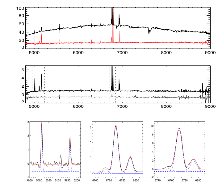
Figure 3: Examples showing intermediate results, reduced spectra, and detailed views of the H$\beta$ and H$\alpha$ emission line regions. In all panels the horizontal axes are in Angstroms and the vertical axes show flux in units of 10E-17 erg/s/cm2/Å. Top panel: The black line shows the spectrum derived for a simulated SDSS aperture in an intermediate reduced data cube (gal20 is shown in this example – arbitrary flux units). The flux calibrated SDSS spectrum itself is shown in red. By matching the simulated spectrum to the SDSS spectrum wavelength by wavelength, see section 3, we can remove both the VIMOS response profile and establish the flux calibration scale. Middle panel: Reduced spectra along two individual spaxels in gal20. The upper line shows an example of a bright spectrum along a central spaxel while the bottom line shows a faint spectrum in a spaxel near the edge of the galaxy. Note that the faint spectrum has been vertically offset by -1.0 for clarity. In the subsequent emission line analysis we only use the two wavelength regions bounded by the dotted lines and is thus not affected by the sky subtraction residuals seen beyond 7000 Å. Bottom panels: Close-ups views of emission line fits in continuum subtracted gal20 spectra. The left and middle panels show the H$\beta$+[OIII] and H$\alpha$+[NII] complex respectively for a spectrum binned in a circular annulus with a radius of $2^{\prime\prime}$. The best-fit is oveplotted in red and the individual best-fit components are shown in blue (with a negative offset for clarity). The centroids and the width of three individual Gaussian components in each panel are tied to each other. That is, we assume that the gas traces the same kinematic features. Hence, we fit only one systemic velocity and dispersion per panel. For comparison the right most panel shows the H$\alpha$+[NII] in the annulus at the largest radius ($10^{\prime\prime}$). Averaging over lines with up to 400 km/s velocity difference at this radius leads to a noticeable broadening but the overall shape remains Gaussian.

4 Results

Before analysing the individual spaxels/spectra we first examine radially averaged, higher S/N measurements by combining spectra in circular annuli. In each data cube we centre the annuli on the centre of continuum flux distribution. The width of the annuli is one spaxel (0.67 arcsec) and their radii range from 1 to 19 spaxels in steps of 2 spaxels. The emission lines in the radially averaged spectra are analysed in exactly the same way as the individual spaxels described in the previous section.

4.1 H$\alpha$/ colour profiles

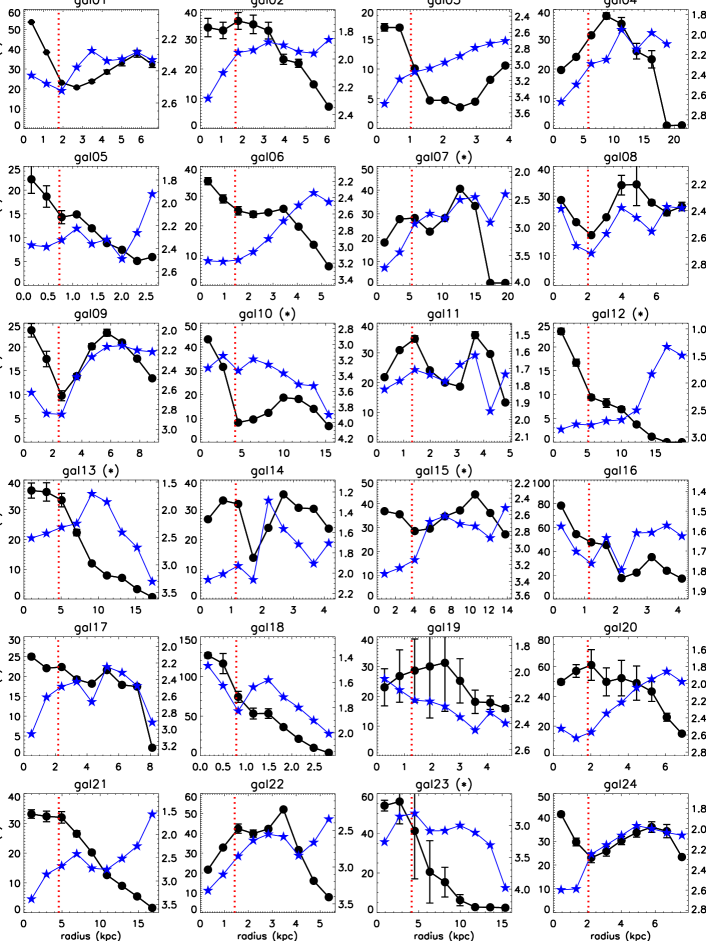
Figure 4: The radial profiles of EW[H$\alpha$] for each of the galaxies in our sample (black lines and circles). These quantities are derived in circular annuli of increasing radius. The dotted, red, vertical line shows the size of a SDSS fibre. The large variety in profile shapes illustrates that H$\alpha$ emission and derived properties, such as star formation rate, are very sensitive to the choice of aperture. The error bars are propagated from errors in the fit. The blue lines and stars show the $u-i$ colour profiles derived from the SDSS images over the same annuli as the equivalent width profiles. The colour scales are shown on the right of each panel: note that this scale is inverted to qualitatively match EW[H$\alpha$]. Galaxies labelled with an asterisk are radio or BPT AGN, see text.

Figure 4 shows the EW[H$\alpha$] profiles derived by simultaneously fitting three Gaussians to the H$\alpha$+ [NII] lines in the summed spectra of each annulus. The errors are propagated from errors in the fit. H$\alpha$ emission is detected out to a radius ranging between 3 and 20 kpc. For comparison, the SDSS fibre size corresponds to 0.35–2.8 kpc depending on the redshift of the galaxies. Thus, we trace on average the emission line flux out to a radius $\sim$10 times that of the SDSS fibre size.

As the profile shapes are often slowly declining with radius or even roughly constant, most of the H$\alpha$ flux in these systems is missed by the SDSS spectra. For a qualitative comparison, u-i colour profiles derived from the SDSS images and binned in the same annuli as the emission, are also shown in this figure. These will be discussed further in section 5.1.

4.2 BPT

Line ratio diagnostics are commonly employed to distinguish galaxies with ionized gas consistent with HII regions from those requiring a harder ionization field likely associated with the narrow line region of an active galactic nuclei (AGN), although some of the parameter space might also be consistent with radiation associated with shocks and starbursts (Kewley et al, 2001, Sarzi et al, 2010). Kauffmann et al. 2003 (K03 hereon) and B04 have applied such diagnostics to the SDSS spectra, applying semi-empirical divisions in the $\frac{\rm[OIII]\lambda 5007}{H\beta}$ versus $\frac{\rm[NII]\lambda 6584}{H\alpha}$ “BPT” diagram (Baldwin, Phillips & Terlevich, 1981) to classify galaxies into star-forming (left of the empirical line marking the tight locus occupied by most galaxies), AGN including LINERS (right of the Kewley et al. (2001) line calibrated to maximal models of starburst galaxies) and composite (in between the two lines) types.

For radial bins where all four emission lines can be fit, we have measured these ratios in our data. In Fig. 5 the resulting line ratio tracks are overplotted in colour on a greyscale background showing the distribution of fibre-based SDSS measurements presented by K03 and B04. The empirical lines used by K03 and Kewley et al. (2001) to divide pure star forming galaxies from AGN and composite galaxies are overplotted in black. The direction of increasing radius traced by the line ratio tracks is from red to blue, with crosses marking measurements for the individual annuli (radially binned with an annulus width of 2 pixels, corresponding to 1.5″). To verify our calibration we have also derived the line ratios directly from the spectra in the SDSS database. These are shown as yellow diamonds. They are generally located close to the red, low radius part of each track as expected, since they cover only the central 3″. As an additional check we also plot the ratios obtained using the line fluxes derived by B04. These are shown as black diamonds, and are located very close to the yellow diamonds with small differences possibly due to differences in the correction for underlying stellar balmer line absorption.

It is clear that our sample includes both galaxies for which the ionization state is consistent with that expected in HII regions (presumably normal star-forming galaxies) and those for which line ratios require a component of harder ionizing radiation. As noted in Gerssen et al. 2009, gal15 contains an extended narrow line region (ENLR), requiring a harder ionizing radiation component impacting the ionized gas out to large $\sim 9$kpc radii. Indeed, all galaxies requiring harder ionization (7, 12, 15, 23) remain in that part of the diagram out to relatively large radii! Our targets were not in any way selected to contain ENLRs, or even AGN. Therefore, at least based upon our small, high EW[H$\alpha$] sample, ENLRs appear to be a common phenomenon such that emission lines at large radii (i.e. $\sim 1-10$ kpc) are not independent of nuclear properties and as such do not trace only star formation.

Ionizing radiation in galaxies whose tracks remain to the left of the K03 dividing line should be dominated by star formation in HII regions. Consistent with this hypothesis, most of these galaxies follow tracks along this star forming locus, verifying the consistency of line ratios for resolved subsections of galaxies and radial bins which extend far beyond the SDSS fibres. In galaxies 1,2,4,6,11,13,14,16,17,19,20,22 and 24, the data is consistent with a movement to larger $\frac{\rm[OIII]\lambda 5007}{H\beta}$ and smaller $\frac{\rm[NII]\lambda 6584}{H\alpha}$ (up and to the left) along the locus with increasing radius. This is consistent with expectations, since in this direction metallicity is mostly decreasing and ionization parameter increasing (see Fig. 4 of Levesque, Kewley & Larson, 2010). Galaxies 2 and 5 move off the locus at large radii, where the signal to noise becomes low in [NII] and [OIII] lines. Galaxy 18 presents a reverse track, moving to smaller $\frac{\rm[OIII]\lambda 5007}{H\beta}$ and larger $\frac{\rm[NII]\lambda 6584}{H\alpha}$ at larger radii. This galaxy is unusual, with a double nucleus probably related to a late merger stage. During a merger unusual gradients in metallicity and ionization parameter should not be unexpected.

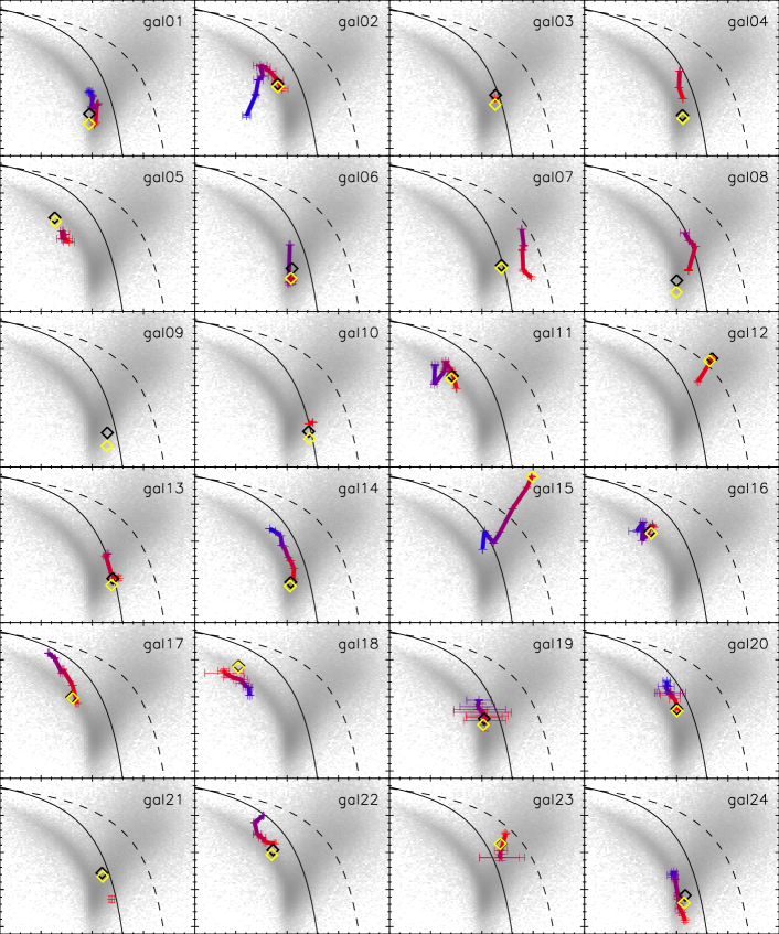
Figure 5: The emission line flux ratios measured in the same annuli as in Fig 4 are shown here as ’tracks’ on top of SDSS-derived BPT diagrams. The latter are taken from single-aperture measurements of some 500,000 galaxies in the SDSS database (B04). The radius increases by 2 spaxels for successive points along the track. The direction of increasing radius is along the red to blue colour gradient for each track. Although not selected as such, several systems have (hidden) AGN activity. This is particularly striking in gal15 (Gerssen et al. 2009). To verify our calibration we have also derived the line ratios directly from the spectra in the SDSS database. The results are shown as the yellow diamonds. They are generally located close to the start of each track as expected. The black diamonds depict the line ratios obtained using the B04 line flux measurements. The dashed and solid lines show the boundary between star forming and AGN systems as derived by Kewley et al. (2001) and Kauffmann et al. (2003) respectively.

4.3 Maps

In Fig. 9 we present maps derived from the emission line analysis to the H$\alpha$$+$[NII] lines in all individual spaxels/spectra. We interactively inspected the best fit results in all spaxels and flagged the poor fits. The best-fit continuum and emission-line fluxes are shown in columns one and two respectively. The next two columns show kinematical maps derived from the line fits, the velocity fields in column three and the dispersion maps in column four. The size of the maps is the FoV of VIMOS on the sky, 27 by 27 arcsec, and is thus the same in all panels and for all galaxies shown. The horizontal black bars in column one are five kpc long and are useful to gauge the relative physical sizes of the galaxies in our sample (see also Table LABEL:t:sample). In all maps we only plot those spaxels which are not flagged and have Ha line flux ratio $\geq 3$.

4.3.1 Continuum maps

The colour SDSS images shown in Figure 1 have the same size and orientation as the maps in Figure 9 and can be compared directly to the continuum maps. Galaxies gal13, gal14 and gal16 have a nearby foreground star in their colour images that is also clearly noticeable in their continuum maps. The foreground stars in gal11 and gal17 are not seen in the continuum maps as these regions were rejected in the line-fitting analysis (too low S/N to fit emission lines).

4.3.2 H$\alpha$ line-flux maps

The galaxies in our sample were selected to be moderately gas-rich, H$\alpha$ EW $\geq 20$. Their spiral arm structure, apparent in Figure 1 and to a lesser extent in our continuum maps, can be readily traced in the H$\alpha$ line-flux maps. In particular gal11 and gal24 display a striking number of H$\alpha$ clumps that partially trace the flocculent spiral arms in these two systems. Similarly, the grand design spirals structure in galaxies gal06, gal07, gal10 and gal13 is also visible in the line-flux maps. And in systems that are close to edge-on the H$\alpha$ distribution traces spiral arm features where non can be seen in broad band images. The linear structure of H$\alpha$ clumps seen in gal17, for example, resembles an edge-on version of gal24.

Most off-center H$\alpha$ emission is clumpy, and several systems in particular, i.e. gal01, gal08, gal09, gal11, gal14, gal15, gal17, gal18, gal22, contain clear off-center H$\alpha$ clumps. We measure the flux of off-centre clumps in these galaxies, fitting the H$\alpha$ line for summed spaxels – the dominant error is the size of the clump. These are recorded along with estimated star formation rates using the relation of Kennicutt 1998 (no dust correction) in Table 2. In the cases of gal11 and gal18 we record the flux for all clumps, as there is no obvious nucleus. These flux measurements can be compared to the total and nuclear (SDSS aperture) fluxes presented in table LABEL:t:flux (see section 5.1). In all cases the clumps are at least as luminous in H$\alpha$ as the nucleus of the galaxy. Thus, whilst most galaxies in our sample contain H$\alpha$ bright nuclei, this does not preclude the existence of brighter star forming regions in the disk. In fact, these clumps are bright enough to drive a constant or increasing EW[H$\alpha$] with radius in azimuthally averaged annuli, for many of the galaxies containing bright off-center clumps, as shown in Fig 4.

Table 2: Integrated off-centre clumps: H$\alpha$ emission flux, and star formation estimated using the relation of Kennicutt 1998 (no dust correction).

Name/clump	Flux	SFR
	$10^{-17}ergs^{-1}cm^{-2}$	$M_{\odot}yr^{-1}$
gal01	755	0.120
gal08	1171	0.241
gal09	1052	0.318
gal11SE	290	0.025
gal11W	258	0.022
gal11N	344	0.029
gal14	2149	0.022
gal15	2503	2.040
gal18E	2059	0.060
gal18W	5710	0.167
gal20	2459	0.419
gal22E	523	0.053
gal22W	510	0.052

4.3.3 H$\alpha$ velocity fields

The best-fit gas line-of-sight velocities are shown in column three. In general the H$\alpha$ velocity maps are consistent with well defined, regular rotation. Even in systems that appear close to face-on in the SDSS images and continuum maps, e.g. gal06, ga08 and gal11, low amplitude rotation is still discernible. In most galaxies in our sample the observed velocity amplitudes lie in the range of 100 to 200 km/s. In section 4.4 we quantify the velocity amplitudes and use them to derive a dynamical estimate of the enclosed mass in these systems.

4.3.4 H$\alpha$ dispersion maps

The velocity dispersion maps shown in column four are corrected for instrumental broadening by re-deriving our combined data cubes without sky subtraction, and then fitting a Gaussian function to the 5577Å sky line in order to measure the instrumental dispersion for each spaxel. This value is typically consistent with the measured H$\alpha$ dispersion in the outer regions of galaxies, indicating that these spaxels are dominated by instrumental dispersion. We subtract this from the measured H$\alpha$ width in quadrature, setting to 0 in cases where the measured dispersion is lower than the instrumental dispersion. Some galaxies show significant peaks in dispersion, centred on the galaxy nucleus. We discuss this further in section 5.2.

4.4 Enclosed mass

The velocity fields shown in column 3 of Fig. 9 can be used to obtain dynamical constraints on the enclosed mass in these galaxies. Building sophisticated kinematical models is outside the scope of this paper. Instead we obtain enclosed mass estimates by fitting the velocity fields with a simple, infinitely thin circular disk model. The radial velocity distribution in this toy model is characterized by a velocity that rises linearly from 0 km/s at the center to a constant value, $V_{\rm circ}$, at a break radius, $R_{\rm break}$ and is constant thereafter. The centre, position angle and inclination of the velocity field model are also free parameters. The best fit model is found simply by varying the five model parameters over a five-dimensional grid. For each grid point we compute the summed squared residual value of the difference between the model and the observed velocity field. As the best fit model we take the grid point with the minimum residual value.

Not all H$\alpha$ velocity fields in our sample are sufficiently well defined, or sufficiently well sampled for our simple toy model to produce an acceptable fit. The aim of this toy model is to estimate a dynamical mass using the best-fit circular velocity at a reference radius of 10 kpc. As we do not attempt to accurately constrain the central behaviour of the velocities the exact value of the break radius is not relevant here as long as $R_{\rm break}<10$ kpc. For those galaxies in our sample that meet this criterion we list the estimated dynamical mass in table LABEL:t:mass.

As a comparison, we list the stellar masses derived for K03 where these are available. They derive stellar mass to light ratios using the D4000Å and H$\delta$ absorption features within the SDSS fibre, and apply this to the total z-band luminosity. To make a fair comparison, we compute an aperture correction by measuring the fraction of z-band flux within a central 10kpc aperture placed on the SDSS z-band images, masking nearby objects. The final column in table LABEL:t:mass lists the stellar masses within 10kpc by applying this correction factor.

Figure 6 shows the dynamical versus stellar masses within an aperture of 10kpc. Solid and dotted lines respectively illustrate the locus of objects with 100% and 10% of the total mass in stars. Acknowledging uncertainties in both measurements, all galaxies are consistent with values in between these two extremes. Interestingly, there is no significant dependence of the fraction of mass in stars, on the mass itself for these measurements.

Table 3: Column 2 lists the enclosed total mass within 10kpc for those galaxies whose H$\alpha$ velocity fields can be fit with a simple model, see text. The third column lists the total stellar masses derived by K03. The fourth column corrects this to an aperture of 10kpc by computing the fraction of z-band light within this radius.

Name	log $\frac{M_{dyn}}{M_{\odot}}(R\leq 10kpc)$	log $\frac{M_{*}}{M_{\odot}}$ (K03)
		total	$(R\leq 10kpc)$
gal01	9.9	9.333	9.04
gal02	10.0	9.872	9.73
gal03	–	–	–
gal04	–	10.930	10.53
gal05	9.2	8.569	8.38
gal06	–	9.575	9.47
gal07	–	10.874	10.27
gal08	–	10.016	9.83
gal09	10.1	10.565	10.34
gal10	–	11.022	–
gal11	8.9	8.817	8.59
gal12	10.2	10.661	10.00
gal13	–	10.964	10.41
gal14	10.1	9.614	9.57
gal15	–	–	–
gal16	10.2	9.239	9.20
gal17	10.4	10.041	9.60
gal18	9.8	–	–
gal19	9.9	9.537	9.44
gal20	10.4	10.337	10.15
gal21	10.5	10.925	10.45
gal22	10.3	–	–
gal23	–	11.220	10.87
gal24	10.7	10.585	10.39

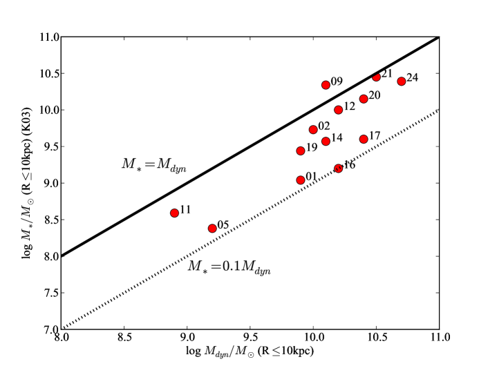
Figure 6: Dynamical mass from our toy model within 10kpc versus stellar mass from K03, scaled by z-band flux to that within a 10kpc circular aperture. Only galaxies for which these two parameters could be derived are included. The solid (dotted) line shows where the stellar mass accounts for all (one-tenth) the total mass within 10kpc. Our galaxies typically lie between these two lines, and this ratio shows no mass dependence.

5 Discussion

5.1 Radial gradients and SDSS aperture effects

Figure 4 illustrates the wide range of EW[H$\alpha$] and colour profiles for galaxies in our sample. The (u-i) colour profiles of some objects (e.g. 08,18) trace their EW[H$\alpha$] profiles closely, suggesting that both trace the same features via the ratio of young to old stars.

However most cases are not so simple: u-band light traces stars much less massive and older than the very massive and young stars traced by H$\alpha$ recombination (effectively the instantaneous SFR). H$\alpha$ emission is also highly sensitive to dust extinction in HII regions and can be triggered through different sources of ionizing radiation (e.g. AGN), whilst the slightly older stars dominating the u-band light will have migrated out of HII regions and are therefore sensitive mostly to diffuse dust absorption. At regions of low surface brightness and low star formation density (e.g. at large radius), the stochastic nature of star formation might lead to a significant excess of u-band light over that seen in the instantaneous SFR via H$\alpha$. These and other effects must lead to the mismatch in the colour and H$\alpha$ profiles of most galaxies in our sample.

The VIMOS data allow us to directly quantify aperture corrections by comparing the H$\alpha$ line flux in the SDSS fibre to the total line flux of the galaxy. The derived line fluxes are listed in table LABEL:t:flux and have been corrected for absorption as described in section 3.1. We simulate the SDSS apertures on our VIMOS data cubes using the procedure described in section3. The derived H$\alpha$ line flux in the simulated SDSS apertures are listed in column 2. For comparison we apply the same line fitting technique to the SDSS spectra themselves, see column 3. The close correspondence between the derived line fluxes validates our data reduction process which used the relative continuum level of the SDSS spectrum to recalibrate our flux scale. The line fluxes derived by B04 in column 4 provide an independent measurement.

The total line fluxes listed in column 5 are obtained by summing the flux from the radial binned spectra. The ratio of the line flux in the simulated SDSS aperture to total flux is tabulated in column 6. While the total flux is a measure within the field of VIMOS, the H$\alpha$ maps in Fig. 9 demonstrate that this encompasses the brighter part of the disk, and any additional contribution to the total H$\alpha$ line flux should be negligible (By design as our selection criteria were constructed with that purpose in mind).

The large variation in this ratio demonstrates that generic aperture corrections are of limited value when working with individual galaxies. For instance, the ratios show no correlation with the factors derived by B04 to correct aperture SFRs. These were derived by assuming a simple mapping of galaxy colour to emission line derived SFR (calibrated using SDSS spectra with the inherent aperture effects). This mapping is clearly unreliable for individual galaxies, as suggested by Figure 4. In many cases the central colour profile is especially deviant from the EW[H$\alpha$] profile - for example due to AGN contamination or differential dust extinction.

Figure 7 shows the aperture correction for H$\alpha$ line flux calculated for our data plotted against the SFR aperture correction of B04 Even ignoring the likely AGN (radio or BPT, shown in green - see section 5.2), there is no correlation between the two corrections, indicating that these colour-based corrections are inaccurate for individual galaxies. However we note that our sample covers only galaxies with EW[H$\alpha$]${}_{fibre}>20$Å and the correction to H$\alpha$ flux need not equate exactly to the ‘SFR’ correction.

As all points, except one AGN, fall to the left of the 1:1 relation in Figure 7, it appears that B04 underestimate the correction on average. To quantify this we have examined the distribution of y-axis value divided by x-axis value (the ratio of the aperture fractions) for non-AGN only. We find that this distribution has a mean at ratio 2.5, and scatter of 175%. Thus the correction applied by B04 appears – on average – underestimated, assuming that the dust correction is not larger in the outskirts of star forming galaxies than in the inner parts. To an order-of-magnitude level, the B04 aperture correction may be valid. However, for individual galaxies, we can say that the systematic error induced by such a correction is a factor 2.5 for star forming galaxies, with even larger random errors, especially where other sources of ionizing radiation are present.

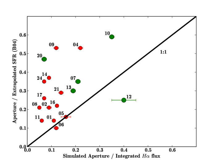
Figure 7: The measured ratio of H$\alpha$ flux measured inside the radius of a SDSS fibre (simulated SDSS fibre) to the total flux including errors (x-axis) plotted against the estimated SFR aperture correction from B04, (y-axis). The green points are the AGN (radio or BPT). The solid black line shows the 1:1 relation. Galaxies 04, 15 and 18 have no SFR measurement from B04.

Table 4: H$\alpha$ line flux in units of $10^{-17}$ erg s^-1 cm^-2. VIMOS has a known spaxel near its centre with a low transmission. This has affected our flux calibration in the central few spaxels of galaxies 03, 19 and 23 through the drizzling step in our reduction Hence, we do not attempt to compute the correction factors for these galaxies.

Name	Simul	SDSS	Brinchmann	Total	Simul/Total	Ap corr fac.
gal01	7741) (1.4)	2032)	210	6905 (225)	0.11 (0.003)	0.14
gal02	438 (44.9)	490	542	4776 (332)	0.09 (0.01)	0.21
gal03		1045	1101	32621 (360)		0.36
gal04	702 (7.5)	703	752	3166 (112)	0.22 (0.01)	0.53
gal05	229 (23.6)	223	244	1422 (21)	0.16 (0.02)	0.16
gal06	546 (28.3)	557	612	4550 (103)	0.12 (0.01)	0.10
gal07	377 (13.4)	394	434	1772 (26)	0.21 (0.01)	0.35
gal08	334 (1.5)	318	347	6268 (379)	0.05 (0.003)	0.21
gal09	877 (58.6)	925	953	7185 (182)	0.12 (0.01)	0.53
gal10	957 (10.4)	1063	1121	2727 (54)	0.35 (0.01)	0.59
gal11	139 (1.1)	165	178	2276 (49)	0.06 (0.001)	0.14
gal12	179 (7.2)	246	259	448 (75)	0.40 (0.05)	0.25
gal13	591 (48.6)	530	580	3137 (49)	0.19 (0.01)	0.30
gal14	1467 (0.1)	1409	1520	16544 (17)	0.09 (0.001)	0.37
gal15	849 (0.1)	1094	–	9853 (12)	0.09 (0.001)	–
gal16	613 (0.1)	648	698	5051 (140)	0.12 (0.003)	0.22
gal17	247 (4.1)	260	275	3632 (52)	0.07 (0.001)	0.26
gal18	1080 (135.3)	1012	1062	10356 (422)	0.10 (0.01)	–
gal19		667	746			0.27
gal20	603 (55.1)	660	708	8383 (1138)	0.07 (0.01)	0.47
gal21	287 (23.2)	285	299	2043 (40)	0.14 (0.01)	0.29
gal22	294 (6.7)	253	273	4293 (60)	0.07 (0.001)	–
gal23		2244	2398			0.32
gal24	441 (18.1)	455	490	6737 (382)	0.07 (0.004)	0.35
1) Simul fibre at SDSS position has flux of 248.
2) SDSS fibre is not on gal01 nucleus.

5.2 AGN

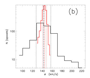
Figure 8: Demonstration of our “dispersion-peak” diagnostics for the strongly dispersion-peaked galaxy gal15. (a) Dispersion profile, for spaxels binned by distance from galaxy centre, where the dispersion ($\sigma$) is the width of the H$\alpha$ line fit for each spaxel, in velocity units, and corrected for instrumental dispersion. The solid and dashed lines represent the median and the 25^th and 75^th percentiles of individual spaxel fits, respectively. We define the radial extent of the central dispersion-peak, $r_{peak\sigma}$ (dashed vertical line), at the maximum radial bin within the 25^th percentile of rises above zero ($\sigma\sim 0$ where the instrumental broadening dominates, and the uncertainty in $\sigma$ is larger than the intrinsic value). (b) Histograms of $\sigma$ for spaxels at $r>r_{peak\sigma}$ (in black) and of $\sigma_{\rm instr}$ – the instrumental dispersion measured using a Gaussian fit to the 5577Å sky line (in red). The centroid of a Gaussian-fit to these histogram (dashed vertical lines) show that the H$\alpha$ line width for these spaxels is consistent with instrumental dispersion and the widths of the Gaussians (dotted lines at $\pm 1-\sigma$) show that the spaxel to spaxel scatter does not result from variation in $\sigma_{\rm instr}$ – instead it probably results from errors in fitting the H$\alpha$ emission line, especially in regions of low flux.

In section 4.2 and figure 5 we saw that whilst most galaxies in our sample have line ratios consistent with pure star forming radiation, four clearly require a harder component of ionizing radiation (7,12,15,23), whilst the line ratio tracks of galaxies 8, 10 and 13 are located above the locus of normal star forming objects, close to the dividing line of (Kauffmann et al. 2003). We will now examine other signatures of energy injection in the central regions of our galaxies and assess the case for nuclear activity, and its influence on the spatially resolved ionized gas and other observables. Nuclear activity may be related to accretion onto a super-massive black hole (an active galactic nucleus, AGN), although certain configurations may also be explained by extreme star formation (starbursts).

The National Radio Astronomy Observatory (NOAO) Very Large Array (VLA) Faint Images of the Radio Sky at Twenty-Centimeters (FIRST: White et al, 97) survey provides the best spatially resolved (1.8″ pixels) radio map of the sky (at the locations of our sources). Radio fluxes are measured with a typical rms of 0.15 mJy, with a 1 mJy source detection threshold. Individual sources have 90% confidence error circles of radius $<0.5\arcsec$ at the 3 mJy level and 1″ at the survey threshold.

Our sources have been matched to the FIRST radio catalogue using a search radius equivalent to the VIMOS field of view. The integrated radio flux (Gaussian fit, White et al. 1997), and offset from the position of the SDSS source, are tabulated in columns 2 and 3 of table LABEL:t:agn. The nuclei of galaxies 10,13,15,20 and 23 contain significant radio sources which can clearly be seen in FIRST images. Small offsets (e.g. galaxy 15) are smaller than the radio source size (despite formal positional errors below 1″) and consistent with typical offsets in H$\alpha$ peak flux from the SDSS position. Radio sources with larger offsets (galaxies 3 and 4), although within the VIMOS field of view, are unlikely to be associated with the galaxy nuclei.

5.2.1 Dispersion-Peaks

The maps illustrating the H$\alpha$ line width (last column of figure 9) demonstrate two regions of interest. For the majority of spaxels the measurement is limited by instrumental resolution: the measured width of the 5577Å sky-line is $\sim 3.3$Å, which corresponds to $\sigma_{\rm instr}\sim 145\rm kms^{-1}$ for a typical galaxy at the wavelength of H$\alpha$. To estimate the intrinsic dispersion, the instrumental dispersion is subtracted in quadrature from the measured dispersion – in these regions the result is close to zero and dominated by measurement errors.

However, in the central regions of many galaxies the H$\alpha$ line width is broader, and resolved (a “dispersion-peak”). The thermal dispersion of gas is $\sigma_{thermal}=\sqrt{\frac{k_{B}T}{\mu m_{p}}}$ which for $T\sim 10^{4}$K results in $\sigma_{thermal}\sim 10~{}kms^{-1}$, much lower than the measured dispersion. Projected circular velocity variations within each spaxel can explain some enhancement, but not much, especially for systems close to face-on. For gas to be so much hotter requires an additional source of thermal or turbulent energy. In central regions it seems likely that this can relate to the presence of an AGN, although supernovae might also provide such energy.

We now compute several diagnostic parameters relating to the dispersion-peak, presented in columns 4-7 in table LABEL:t:agn. To illustrate our method we provide figure 8, demonstrating how these diagnostics are computed for a classic dispersion-peak galaxy, gal15 (presented in Gerssen et al. 2009).

Individual spaxels are binned by radius (distance of the spaxel from the centre, defined as in section 4 to be the position of the continuum peak) in annuli of one pixel width. Where the fit is acceptable, $\sigma$ is the measured width of the H$\alpha$ line for each spaxel, converted to rest-frame velocity units. For the spaxels contained within each radial bin, we then examine the distribution of $\sigma$.

Figure 8, panel (a) shows the median (solid line), and the 25^th and 75^th percentiles (dashed lines) of this distribution versus radial bin. For galaxy 15 this $\sigma$-profile defines a central peak, as seen in the $\sigma$-map of this galaxy (figure 9).

In the outer regions of the galaxy instrumental broadening dominates the measured line dispersion – together with measurement error this means the intrinsic dispersion is consistent with zero. This is seen in the 25^th percentile (lower dashed line) which goes to zero beyond 8″. We use this fact to estimate the extent of the dispersion-peak – $r_{peak\sigma}$ is set to the maximum radial bin before the 25^th percentile goes to zero (effectively $\geq 25\%$ of the spaxels at larger radii have measured dispersion $\sigma\geq\sigma_{\rm instr}$). $r_{peak\sigma}$ is marked with the vertical dashed line in figure 8, panel (a).

Figure 8, panel (b) shows the distribution of measured dispersion ($\sigma_{\rm meas}$) for all spaxels containing H$\alpha$ at $r>r_{peak\sigma}$ (black histogram). The red histogram shows the distribution of $\sigma_{\rm instr}$ measured using the 5577Å sky line for the same spaxels (using a smaller binsize, but renormalized for comparison with the black histogram). The histograms peak at roughly the same value of $\sigma_{\rm meas}$, which demonstrates that the dispersion in these peaks is dominated by the instrumental broadening. To characterize these distributions we fit a Gaussian to each peak. The vertical dashed and dotted lines show the median and $\pm 1-\sigma$ respectively, based on these fits. The distribution of $\sigma_{\rm meas}$ is much broader than that for the instrumental dispersion – this shows that the scatter in $\sigma_{\rm meas}$ is dominated by fitting errors and not by spaxel to spaxel variations in the instrumental dispersion.

Finally, we compute the overall significance of the dispersion-peak. The significance that $\sigma_{i}$ is larger than then the baseline value (computed using the mean dispersion for spaxels at $r>r_{peak\sigma}$ = $<\sigma_{r\geq r_{peak\sigma}}>$) for each spaxel $i$ is:

$$signif_{i}=\frac{\sigma_{i}-<\sigma_{r\geq r_{peak\sigma}}>}{rms(\sigma)}$$ (1)

where the noise $rms(\sigma)$ is estimated by adding in quadrature the scatter from the two distributions in measured and intrinsic sigma (the black and red histograms in figure 8, panel (b)) – this is dominated by the measurement error from the H$\alpha$ emission line fitting process ($\sigma_{\rm meas}$).

The combined significance of the peak is simply:

$$signif(r<r_{peak\sigma})=\sqrt{(}\Sigma_{i=1}^{N}signif_{i}^{2})$$ (2)

for N spaxels with $r<r_{peak\sigma}$.

We also compute the intrinsic velocity dispersion $\sigma_{\rm cen}$ for the central spaxel, by subtracting $\sigma_{\rm instr}$ from $\sigma_{\rm meas}$ in quadrature.

A low amplitude ($\sigma_{\rm cen}$) but greatly extended dispersion-peak such as galaxy 3 is highly significant. Such peaks may result from the projected rotation curve convolved with the seeing.

It is physically more interesting to consider the physical origin of higher dispersion peaks with significant S/N and size ($r_{peak\sigma}$).

Galaxies 10, 15 and 23 contain both significant dispersion-peaks with $\sigma_{\rm cen}\geq 131$km s^-1and nuclear radio sources. Of these, galaxies 15 and 23 also have line ratios in the BPT diagram which require harder ionization radiation, consistent with AGN origin. Galaxies 7, 12 (and possible galaxy 10) have dispersion-peaks and AGN-like line ratios, but no known radio counterpart.

Most importantly, all galaxies with radio counterparts or clear AGN-like line ratios have a central dispersion-peak, whilst all galaxies with no, or very low significance dispersion-peaks have line ratios consistent with a pure HII region ionization field and no radio source. These correlations strongly suggest that the same, or related physical mechanism(s) are responsible for the energy injection which drive all these phenomena (radio power, a hard ionization field and kinematic heating). The most promising candidate energy source is via coupling of an AGN with the surrounding gas. In this case radio emission traces jets during the “on” phase of the jet duty cycle, whilst the surrounding gas is ionized by the hard radiation of the accretion disk, and can be kinematically heated by the jet (e.g. van den Bosch $\&$ van der Marel, 1995; Koekemoer, 1996). And although the H$\alpha$ flux of off-centre clumps is frequently brighter than that in the nucleus, the dispersion is never enhanced in those regions – Fig 9

Whatever the origin, these features are common in our sample (selected only to have fibre EW[H$\alpha$]$>20$Å). Whilst no single selection method picks up all objects, kinematic heating of the central ionized gas (dispersion-peaks) selects a fairly complete subset of radio and BPT-selected sources, as well as sources such as gal09 for which not all emission lines can be measured with a high enough signal to noise ratio.

Table 5: Properties of galaxies which might indicate the presence of an active galactic nucleus (AGN). Columns 2 and 3: “Deconvolved flux” in mJy and offset of radio source from the SDSS optical position, where a galaxy has been matched to a radio source within the FIRST catalogue (White et al. 1997). Note that FIRST fluxes are inexact but our main purpose is to illustrate the presence of radio flux. Columns 4-7: The maps of H$\alpha$ emission line width ($\sigma$, see figures 9-9 final column) have been examined for the presence of a “dispersion-peak” at the galaxy centre, corresponding to ionized gas which is heated to levels at which the H$\alpha$ line is resolved. Parameters describing this peak are presented here, and described in the text (section 5.2). Column 8: Are the line ratios consistent with an ionization field expected for pure HII regions? (Yes/No/?).

Name	FIRST flux	FIRST offset	$\sigma_{\rm cen}$	$\sigma_{\rm instr}$	$r_{\rm peak\sigma}$	signif($r<r_{\rm peak\sigma}$)	BPT pure HII region?
	mJy	$\arcsec$	km/s	km/s	$\arcsec$
gal01	-	-	69	148	3.4	8.7	Y
gal02	-	-	-	148	-	-	Y
gal03	3.16	11.1	47	152	4.0	49.3	Y
gal04	2.06	13.6	60	138	2.0	2.4	Y
gal05	-	-	-	138	-	-	Y
gal06	-	-	25	138	-	-	Y
gal07	-	-	173	135	3.4	30.4	N
gal08	-	-	43	147	6.0	30.9	?
gal09	-	-	121	148	6.0	42.5	Y
gal10	2.72	0.8	146	142	2.7	22.6	?
gal11	-	-	-	142	-	-	Y
gal12	-	-	84	139	1.3	5.3	N
gal13	2.31	0.4	79	141	6.0	18.7	?
gal14	-	-	-	141	-	-	Y
gal15	3.03	2.5	192	144	8.0	81.3	N
gal16	-	-	-	144	-	-	Y
gal17	-	-	8	148	0.7	0.4	Y
gal18	-	-	29	148	-	-	Y
gal19	-	-	-	148	-	-	Y
gal20	3.87	1.3	16	147	1.3	0.7	Y
gal21	-	-	66	140	2.7	7.6	Y
gal22	-	-	-	140	-	-	Y
gal23	6.22	0.7	131	141	4.7	24.9	N
gal24	-	-	-	147	-	-	Y

6 Summary

In this data paper we have presented VIMOS IFU data of 24 galaxies selected from the SDSS database We use our VIMOS maps to quantify the differences in simulated SDSS apertures to integrated H$\alpha$ flux. These flux ratios are uncorrelated with aperture corrections based on simple colour based SDSS extrapolations which are underestimated by a factor $\sim$2.5 on average, with 175% scatter with respect to measured ratios. We have estimated the enclosed dynamical mass from toy model fits to the H$\alpha$ velocity fields finding between 10 - 100% of mass at $<10$ kpc in stars. We examine various signatures of nuclear activity (line ratios, dispersion peaks, radio emission) and find that about half of the galaxies in our sample show no evidence for nuclear activity or non-thermal heating. As our sample of star forming galaxies is spatially well sampled it can be used as a local reference sample for a comparison with high-z galaxies (e.g. the SINS survey, Förster-Schreiber et al. 2009). Lessons should be learned at low redshift where we have the higher spatial resolution, signal to noise, and ancillary data to attribute cause and effect. For instance, ionized gas kinematics are largely driven by non-gravitational processes such as turbulence. The next generation of observatories, including JWST, ALMA and ELTs, will focus on observations of the high redshift Universe. The availability of detailed observations in the nearby Universe will be of great value to facilitate the interpretation of high-z data. High spatial resolution, wide-field IFS surveys of ionized gas providing samples such as the one presented in this paper, are ideally suited to the task of building up local reference samples.

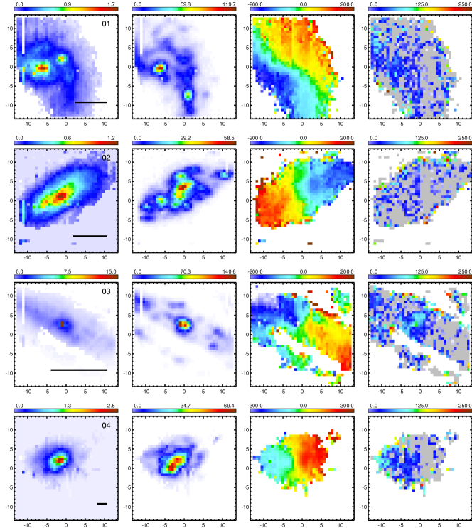
Figure 9: Properties of the 24 SDSS galaxies in our VIMOS IFU sample. The galaxies are plotted in numerical order from top to bottom. The results shown in these panels are derived by fitting the H$\alpha$+[NII] emission lines with a set of three Gaussians. In all maps only those spaxels with SN ratios $\geq 3$ are plotted. The best-fit continuum level maps are shown in column 1 and the H$\alpha$ line flux maps in column 2. Flux is in units of $10^{-17}$ erg s^-1 cm^-2. The velocity fields and velocity dispersion maps in km s^-1 are shown in column 3 and column 4 respectively. Note that in the instrumental dispersion profile has been subtracted in quadrature from the best-fit dispersion measurements. All colour maps are linear and the orientation in each panel is such that North is up and East to the left with the axis scales in arcsec. Spaxels that are grey in column 4 have measured widths that are below the measured sky line widths. (Regions of low flux where fitting errors dominate measurements of dispersion.) The horizontal black bars in the first column are all five kpc long.

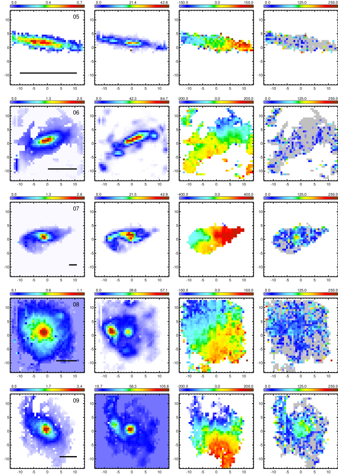
Figure 9: cont.

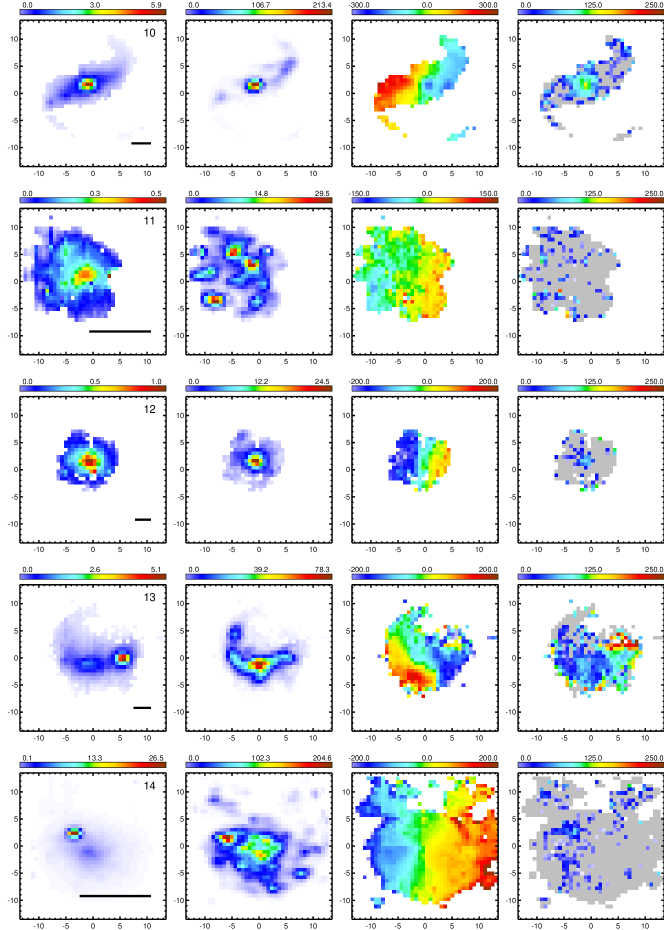
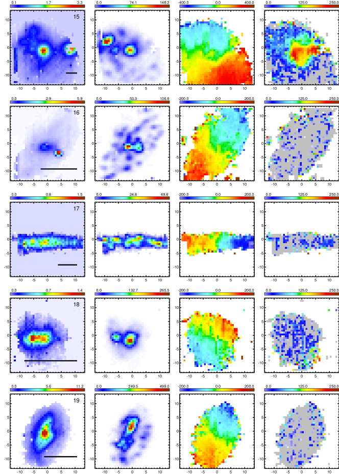
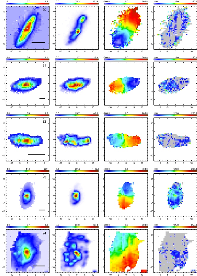
Figure 9: cont.

Figure 9: cont.

Figure 9: cont.

References

- Bacon (2001) Bacon, R., Copin, Y., Monnet, G., Miller, B. W., Allington-Smith, J. R., Bureau, M., Carollo, C. M. et al. 2001, MNRAS, 326, 23
- Baldwin (1981) Baldwin, J. A., Phillips, M. M., Terlevich, R. 1981, PASP, 93, 5
- Becker (2002) Becker, T. 2002, PhD thesis, Astrophysikalisches Institut Potsdam, Germany
- Brinchmann (2004) Brinchmann, J., Charlot, S., White, S. D. M., Tremonti, C., Kauffmann, G., Heckman, T. & Brinkmann, J. 2004, MNRAS, 351, 1151 (B04)
- Bruzual (2003) Bruzual, G. & Charlot, S. 2003, MNRAS, 344, 1000
- Epinat (2010) Epinat, B., Amram, P., Balkowski, C. & Marcelin, M. 2010, MNRAS, 401, 2113
- Forster (2009) Förster-Schreiber, N. M., Genzel, R., Bouché, N., Cresci, G., Davies, R., Buschkamp, P., Shapiro, K., et al. 2009, ApJ, 706, 1364
- Fruchter & Hook (2002) Fruchter, A. S., & Hook, R. N. 2002, PASP, 114, 144
- Gallazzi (2006) Gallazzi, A., Charlot, S., Brinchmann, J. & White, S. D. M. 2006, MNRAS, 370, 1106
- Garrido (2002) Garrido, O., Marcelin, M., Amram, P. & Boulesteix, J. 2002, A&A, 387, 821
- Gerssen (2009) Gerssen, J., Wilman, D. J., Christensen, L., Bower, R. G., Wild, V. 2009, MNRAS, 393L, 45
- Kauffmann (2003) Kauffmann, G., Heckman, T. M., White, S. D. M., Charlot, S., Tremonti, C., Peng, E. W., Seibert, M. et al. 2003, MNRAS, 341, 33 (K03)
- Kauffmann (2003b) Kauffmann, G., Heckman, T. M., Tremonti, C., Brinchmann, J., Charlot, S., ; White, S. D. M., Ridgway, S. E. et al. 2003 MNRAS, 346, 1055
- Kennicutt (1998) Kennicutt, R., 1998, ARAA, 36, 189
- Kewley et al. (2001) Kewley, L. J., Dopita, M. A., Sutherland, R. S., Heisler, C. A., Trevena, J. 2001, ApJ, 556, 121
- Kewley (2005) Kewley, L. J., Jansen, R. A. & Geller, M. J. 2005, PASP, 117, 227
- Levesque (2010) Levesque, E. M., Kewley, L. J. & Larson, K. L. 2010, AJ, 139, 712
- Mattsson (2009) Mattsson, L., Bergvall, N. 2009, IAU symposium 254, eds. Andersen, J., Bland-Hawthorn, J., Nordström, B.
- Koekemoer (1996) Koekemoer, A. M., 1996, PhD. thesis, Australian National Univ.
- Pych (2004) Pych, W. 2004, PASP, 116, 148
- rix (1992) Rix, H.-W., & White, S. M. 1992, MNRAS 254, 389
- Rosales-Ortega (2010) Rosales-Ortega, F. F., Kennicutt, R. C., Sánchez, S. F., Diaz, A. I., Pasquali, A., Johnson, B. D., Hao, C. N. 2010, MNRAS, 405, 735
- Sanchez (2005) Sánchez, S. F., Becker, T., B. Garcia-Lorenzo, B., Benn, C. B., Christensen, L., Kelz, A., Jahnke, K., Roth, M. M. 2005, A&A 429, L21
- Sanchez (2010) Sánchez, S. F., Kennicutt, R. C., Gil de Paz, A., Van den Ven, G., Vilchez, J. M., Wisotzki, L.; Walcher, J. et al. 2010 arXiv1012.3002S
- sazri (2010) Sarzi, M., Shields, J. C., Schawinski, K., Jeong, H., Shapiro, K., Bacon, R., Bureau, M., Cappellari, M. Davies, R. L., de Zeeuw, P. T. et al. 2010, MNRAS, 402, 2187
- Tremonti (2004) Tremonti, C. A. et al. 2004, ApJ, 613, 898
- van den Bosch van der Marel (1995) van den Bosch, F. C. and van der Marel, R. P., 1995, MNRAS, 274, 884
- Walcher (2009) Walcher, C. J., Coelho, P., Gallazzi, A. & Charlot, S. 2009, MNRAS, 398L, 44
- Weilbacher (2009) Weilbacher P. M., Gerssen J., Roth M. M., Böhm P., Pécontal-Rousset A., 2009 In: ”Astronomical Data Analysis Software and Systems XVIII”, eds. D. A. Bohlender et al., ASP Conf. Ser. 411, 159.
- White (1997) White, R. L., Becker, R. H., Helfand, D. J., Gregg M. D. 1997, ApJ 475, 479
- Wilman (2005) Wilman, D. J., Balogh, M. L., Bower, R. G., Mulchaey, J. S., Oemler, A., Carlberg, R. G., Eke, V. R., Lewis, I., Morris, S. L. & Whitaker, R. J. 2005, MNRAS, 358, 88
- York (2000) York, D. G. et al. 2000, AJ, 120, 1579