An Extended Excursion Set Approach to Structure Formation in Chameleon Models

Abstract

In attempts to explain dark energy, a number of models have been proposed in which the formation of large-scale structure depends on the local environment. These models are highly non-linear and difficult to analyse analytically. $N$-body simulations have therefore been used to study their non-linear evolution. Here we extend excursion set theory to incorporate environmental effects on structure formation. We apply the method to a chameleon model and calculate observables such as the non-linear mass function at various redshifts. The method can be generalized to study other obervables and other models of environmentally dependent interactions. The analytic methods described here should prove useful in delineating which models deserve more detailed study with $N$-body simulations.

1 Itntroduction

One of the most challenging questions in contemporary physics is the nature of the dark energy, which is believed to be driving the accelerating expansion of the Universe (Riess et al., 1998; Perlmutter et al., 1999). Copeland et al. (2006) present a comprehensive review of theoretical models to explain the apparent acceleration of the Universe. However, at present there is no compelling evidence for any new physics other than the addition of a cosmological constant to the Einstein field equations.

Models of dark energy can be broadly placed into two categories. In the first, the dark energy affects the expansion rate of the Universe but does not interact directly with the dark matter. Examples of this type of model include the standard $\Lambda$CDM paradigm and quintessence models (Wang et al., 2000). In the second category, the dark energy and matter (both dark and baryonic) interact with each other with an interaction strength which may depend on the local environment. Examples include the chameleon coupled scalar field model (Khoury & Weltman, 2004; Mota & Shaw, 2007), $f(R)$ gravity (Carroll et al., 2005), the environmentally dependent dilaton model (Brax et al., 2010) and also the symmetron model (Hinterbichler & Khoury, 2010).

The possibility of environmentally dependent interactions needs to be considered when relating laboratory measurements to cosmological scales. Consider, for example, a scalar field coupled to matter. The scalar field could mediate a ‘fifth force’ between matter particles. Current laboratory experiments and Solar System tests have shown that such a fifth force must be either extremely weak or short-range (less than about a millimetre) (Will, 2006). However, it is possible that the strength and range of the fifth force depend on the environment so that locally, where the matter density is high, it is strongly suppressed, and it is restored in empty environments. In this situation, laboratory experiments cannot constrain a fifth force that may have observational consequences on cosmological scales.

Analytical models of structure formation on galaxy and cluster scales are notoriously difficult even in the case of standard Newtonian gravity. The evolution of structure in models with environmentally dependent interactions is even more complicated because the fifth force itself is highly non-linear. Consequently, studies so far have relied on full $N$-body simulations (Li & Zhao, 2009, 2010; Li & Barrow, 2011; Li, 2011; Li, Mota & Barrow, 2011; Li et al., 2011; Zhao, Li & Koyama, 2011a; Brax et al., 2011; Davis et al., 2011; Oyaizu, 2008; Oyaizu et al., 2008; Schmidt et al., 2009).

However, large $N$-body simulations require supercomputing resources and are time consuming. They can be justified for testing physically well motivated models such as the $\Lambda$CDM model, which contains few parameters, many of which are now well constrained experimentally, see e.g., Komatsu et al. (2011). Models with a fifth force, on the other hand, span a wide parameter space reflecting our lack of knowledge of the underlying physics. It is difficult to sample a large parameter space using full $N$-body simulations, hence the need for an analytic description of structure formation that can, at least, isolate regions of parameter space that merit further investigation using simulations.

Semi-analytical models, such as excursion set theory (see Zentner (2007) for a recent review), have been developed as alternatives to full $N$-body simulations and shown to agree with the latter well. The excursion set approach has been generalised to some non-standard structure-formation scenarios (Martino et al., 2009; Parfrey et al., 2011). However, these studies do not consider the case of environmentally dependent interactions.

The aim of this paper is to generalise the excursion set approach to take account of environmentally dependent interactions explicitly. As we will see, non-linear collapse of structures could be very different in different environments, and indeed the environments themselves evolve in time as well. We will first specify the environments using what we call the fixed-scale approximation, then use a simplified model to study spherical collapse within these environments. We then calculate observable properties by averaging over the distribution of environments. In this paper we have chosen the chameleon model as a working example, but the methods developed are more general and with suitable changes can be applied to other models with environmentally dependent interactions. The theoretical framework developed here can therefore be used to quickly estimate the parameter ranges of any specific theory that may have interesting (and potentially testable) consequences on structure formation.

The layout of this paper is as follows. We introduce the basic formulae for a chameleon-like coupled scalar field (our working example) in § 2 and summarise the spherically symmetric solutions which will be used later to study the spherical collapse of overdensities. § 3 presents the main results of this paper. We introduce the traditional excursion set theory in § 3.1 and in § 3.2 we show how the environmental dependence in the chameleon model can be approximated using only two variables. § 3.4 describes a generalised spherical collapse model in which an overdensity collapses inside an evolving environment. Finally in § 4 we make an application of the generalized excursion method to a range of chameleon models. Our conclusions are summarized in § 5.

2 The Theoretical Model

This section lays down the theoretical framework for investigating the effects of coupled scalar field(s) in cosmology. We present the relevant general field equations in § 2.1, specify the models analysed in this paper in § 2.2, and then briefly summarise the spherically symmetric solutions in § 2.3.

2.1 Cosmology with a Coupled Scalar Field

The equations presented in this sub-section are derived and discussed in (Li & Zhao, 2009, 2010; Li & Barrow, 2011). They will be used extensively in the rest of this paper and are presented here for completeness and to establish the notation used in later sections.

We start from a Lagrangian density

$${\cal L}={1\over{2}}\left[{R\over\kappa}-\nabla^{a}\varphi\nabla_{a}\varphi\right]+V(\varphi)-C(\varphi){\cal L}_{\rm{DM}}+{\cal L}_{\rm{S}},$$ (1)

in which $R$ is the Ricci scalar, $\kappa=8\pi G$ with $G$ being the gravitational constant, ${\cal L}_{\rm{DM}}$ and ${\cal L}_{\rm{S}}$ are respectively the Lagrangian densities for dark matter and standard model fields. $\varphi$ is the scalar field and $V(\varphi)$ its potential; the coupling function $C(\varphi)$ characterises the coupling between $\varphi$ and dark matter. Given the functional forms for $V(\varphi)$ and $C(\varphi)$ a coupled scalar field model is then fully specified.

Varying the total action with respect to the metric $g_{ab}$, we obtain the following expression for the total energy momentum tensor in this model:

$$T_{ab}=\nabla_{a}\varphi\nabla_{b}\varphi-g_{ab}\left[{1\over 2}\nabla^{c}\nabla_{c}\varphi-V(\varphi)\right]+C(\varphi)T^{\rm{DM}}_{ab}+T^{\rm{S}}_{ab},$$ (2)

where $T^{\rm{DM}}_{ab}$ and $T^{\rm{S}}_{ab}$ are the energy momentum tensors for (uncoupled) dark matter and standard model fields. The existence of the scalar field and its coupling change the form of the energy momentum tensor leading to potential changes in the background cosmology and structure formation.

The coupling to a scalar field produces a direct interaction (fifth force) between dark matter particles due to the exchange of scalar quanta. This is best illustrated by the geodesic equation for dark matter particles

$${{d^{2}\bf{r}}\over{dt^{2}}}=-\vec{\nabla}\Phi-{{C_{\varphi}(\varphi)}\over{C(\varphi)}}\vec{\nabla}\varphi,$$ (3)

where $\bf{r}$ is the position vector, $t$ the (physical) time, $\Phi$ the Newtonian potential and $\vec{\nabla}$ is the spatial derivative. $C_{\varphi}\equiv dC/d\varphi$. The second term in the right hand side is the fifth force and only exists for coupled matter species (dark matter in our model). The fifth force also changes the clustering properties of the dark matter.

To solve the above two equations we need to know both the time evolution and the spatial distribution of $\varphi$, i.e. we need the solutions to the scalar field equation of motion (EOM)

$$\nabla^{a}\nabla_{a}\varphi+{{dV(\varphi)}\over{d\varphi}}+\rho_{\rm{DM}}{\frac{dC(\varphi)}{d\varphi}}=0,$$ (4)

or equivalently

$$\nabla^{a}\nabla_{a}\varphi+{{dV_{eff}(\varphi)}\over{d\varphi}}=0,$$ (5)

where we have defined

$$V_{eff}(\varphi)=V(\varphi)+\rho_{\rm{DM}}C(\varphi).$$ (6)

The background evolution of $\varphi$ can be solved easily given the present day value of $\rho_{\rm{DM}}$ since $\rho_{\rm{DM}}\propto a^{-3}$. We can then divide $\varphi$ into two parts, $\varphi=\bar{\varphi}+\delta\varphi$, where $\bar{\varphi}$ is the background value and $\delta\varphi$ is its (not necessarily small nor linear) perturbation, and subtract the background part of the scalar field equation of motion from the full equation to obtain the equation of motion for $\delta\varphi$. In the quasi-static limit in which we can neglect time derivatives of $\delta\varphi$ as compared with its spatial derivatives (which turns out to be a good approximation on galactic and cluster scales), we find

$$\vec{\nabla}^{2}\varphi={{dC(\varphi)}\over{d\varphi}}\rho_{\rm{DM}}-{{dC(\bar{\varphi})}\over{d\bar{\varphi}}}\bar{\rho}_{\rm{DM}}+{{dV(\varphi)}\over{d\varphi}}-{{dV(\bar{\varphi})}\over{d\bar{\varphi}}},$$ (7)

where $\bar{\rho}_{\rm{DM}}$ is the background dark matter density.

The computation of the scalar field $\varphi$ from the above equation then completes the computation of the source term for the Poission equation

$$\vec{\nabla}^{2}\Phi={{\kappa}\over{2}}\left[C(\varphi)\rho_{\rm{DM}}-C(\bar{\varphi})\bar{\rho}_{\rm{DM}}+\delta\rho_{\rm{B}}-2\delta V(\varphi)\right],$$ (8)

where $\delta\rho_{\rm{B}}\equiv\rho_{\rm{B}}-\bar{\rho}_{\rm{B}}$ and $\delta V(\varphi)\equiv V(\varphi)-V(\bar{\varphi})$ are respectively the density perturbations of baryons and scalar field (we have neglected perturbations in the kinetic energy of the scalar field because it is always very small for our model).

2.2 Specification of Model

As mentioned above, to fully fix a model we need to specify the functional forms of $V(\varphi)$ and $C(\varphi)$. Here we will use the models investigated by Li & Zhao (2009, 2010); Li (2011), with

$$C(\varphi)=\exp(\gamma\sqrt{\kappa}\varphi),$$ (9)

and

$$V(\varphi)={{\Lambda}\over{\left[1-\exp\left(-\sqrt{\kappa}\varphi\right)\right]^{\alpha}}}.$$ (10)

In the above $\Lambda$ is a parameter of mass dimension four and is of order the present dark energy density ($\varphi$ plays the role of dark energy in the models). $\gamma,\alpha$ are dimensionless parameters controlling the strength of the coupling and the steepness of the potentials respectively.

We shall choose $\alpha\ll 1$ and $\gamma>0$ as in Li & Zhao (2009, 2010), ensuring that $V_{eff}$ has a global minimum close to $\varphi=0$ and $d^{2}V_{eff}(\varphi)/d\varphi^{2}\equiv m^{2}_{\varphi}$ at this minimum is very large in high density regions. There are two consequences of these choices of model parameters: (1) $\varphi$ is trapped close to zero throughout cosmic history so that $V(\varphi)\sim\Lambda$ behaves as a cosmological constant; (2) the fifth force is strongly suppressed in high density regions where $\varphi$ acquires a large mass, $m^{2}_{\varphi}\gg H^{2}$ ($H$ being the Hubble expansion rate), and thus the fifth force cannot propagate far. The suppression of the fifth force is even stonger at early times, thus its influence on structure formation occurs mainly at late times. The environment-dependent behaviour of the scalar field was first investigated by Khoury & Weltman (2004); Mota & Shaw (2007), and is often referred to as the ‘chameleon effect’.

2.3 Solutions in Spherical Symmetric Systems

In this subsection we summarise the solutions to the radial profile of the scalar field $\varphi$ in a spherically symmetric top-hat overdensity with radius $R_{\rm TH}$, and (constant) matter density $\rho_{\rm in}$ ($\rho_{\rm out}$) inside (outside) $R_{\rm TH}$. Such a spherically symmetric system will be used to model dark matter halos later. More details concerning these solutions can be found in Khoury & Weltman (2004).

If $\rho_{\rm in}=\rho_{\rm out}$, namely the mater density is the same everywhere, then $\varphi$ will be constant across the whole space and its value simply minimises the effective potential $V_{eff}$. When $\rho_{\rm in}\neq\rho_{\rm out}$, $V_{eff}$ is minimised by $\varphi_{\rm in}$ and $\varphi_{\rm out}$ inside and outside $R_{\rm TH}$ respectively, while $\varphi$ will develop a non-trivial radial profile.

Suppose we go towards the centre of the sphere from outside. If the difference between $\varphi_{\rm in}$ and $\varphi_{\rm out}$ is small, then $\varphi$ will settle to $\varphi_{\rm in}$ (from $\varphi\sim\varphi_{\rm out}$ outside) soon after we enter the sphere; if, on the other hand, the difference is large, then $\varphi$ may never settle to $\varphi_{\rm in}$ even at the centre of the sphere. Khoury & Weltman (2004) give an estimate of the distance $\Delta R$ that is needed for $\varphi$ to settle to $\varphi_{\rm in}$ from $R_{\rm TH}$:

$$\frac{\Delta R}{R_{\rm TH}} = \frac{\sqrt{\kappa}\varphi_{\rm out}-\sqrt{\kappa}\varphi_{\rm in}}{6\gamma\Phi_{\rm TH}},$$ (11)

where $\Phi_{\rm TH}$ is the Newtonian potential at the surface of the sphere:

$$\Phi_{\rm TH}\ =\ \frac{\kappa}{8\pi}\frac{M_{\rm TH}}{R_{\rm TH}}\ =\ \frac{\kappa}{6}\rho_{\rm in}R^{2}_{\rm TH},$$ (12)

and $M_{\rm TH}\equiv\frac{4}{3}\pi R^{3}_{\rm TH}\rho_{\rm in}$ is the mass enclosed within the sphere. Using this, Eq. (11) can be re-expressed as

$$\frac{\Delta R}{R_{\rm TH}} = \frac{\varphi_{\rm out}-\varphi_{\rm in}}{\gamma\sqrt{\kappa}\rho_{\rm in}R^{2}_{\rm TH}}.$$ (13)

Khoury & Weltman (2004) present the solutions to $\varphi$ in two regimes. In the thin-shell regime, where $\Delta R\ll R_{\rm TH}$, the solution is approximately

$$\varphi(r)$$ (17)

$$= \left\{\begin{array}[]{ll}\varphi_{\rm in},&\hbox{$r\in[0,R_{0}]$;}\\ \varphi_{\rm in}+\frac{\sqrt{\kappa}\gamma}{3}\rho_{\rm in}\left[\frac{r^{2}}{2}+\frac{R^{3}_{0}}{r}-\frac{3}{2}R^{2}_{0}\right],&\hbox{$r\in[R_{0},R_{\rm TH}]$.}\\ \varphi_{\rm out}-\frac{\Delta R}{R_{\rm TH}}\frac{\sqrt{\kappa}\gamma\rho_{\rm in}R^{3}_{\rm TH}}{r}e^{-m_{\rm out}\left(r-R_{\rm TH}\right)},&\hbox{$r\in[R_{\rm TH},\infty]$;}\\ \end{array}\right.$$

in which $R_{0}\in\left(0,R_{\rm TH}\right)$ and $R_{\rm TH}-R_{0}\ll R_{\rm TH}$; $m_{\rm out}$ is the effective mass of the scalar field outside the sphere, which is given by

$$m_{\rm out}^{2} \equiv \frac{d^{2}V_{eff}\left(\varphi_{\rm out}\right)}{d\varphi^{2}}.$$ (18)

In the thick-shell regime, where $\Delta R>R_{\rm TH}$, the solution is approximately

$$\varphi(r)$$ (21)

$$= \left\{\begin{array}[]{ll}\varphi_{\rm out}-\frac{3}{\sqrt{\kappa}}\gamma\Phi_{\rm TH}+\frac{1}{6}\gamma\sqrt{\kappa}\rho_{\rm in}r^{2},&\hbox{$r\in[0,R_{\rm TH}]$;}\\ \varphi_{\rm out}-\frac{\sqrt{\kappa}\gamma\rho_{\rm in}R^{3}_{\rm TH}}{3r}e^{-m_{\rm out}\left(r-R_{\rm TH}\right)},&\hbox{$r\in[R_{\rm TH},\infty]$.}\\ \end{array}\right.$$

Physically, if $\varphi$ has developed a thin shell near the edge of the spherical overdensity, then from Eq. (17) we can see that only a fraction $\Delta R/R_{\rm TH}$ of the total mass enclosed in $R_{\rm TH}$ contributes to the fifth force on a test particle at the edge. This means that the fifth force from the matter inside the sphere is strongly screened. In the thick-shell regime the fifth force is not screened.

Note that in the thick shell regime at the edge of the halo we have

$$\frac{C_{\varphi}}{C}\nabla\varphi=\gamma\frac{d}{dr}\left[\sqrt{\kappa}\varphi(r)\right]=-2\gamma^{2}\frac{d\Phi_{\rm TH}}{dr},$$ (22)

which indicates that the magnitude of the fifth force is $2\gamma^{2}$ times that of gravity, and its effect is to rescale the Newton’s constant by $1+2\gamma^{2}$.

3 Analytical Method for Structure Formation

Having reviewed the chameleon model and the solutions in spherically symmetric top-hat overdensities, let us now turn to excursion set theory (Bond et al., 1991), which was developed to study structure formation in cold dark matter scenarios. We will generalise the excursion set approach to the chameleon model, where the dark matter particles experience an extra, environment-dependent, fifth force.

3.1 Excursion Set Theory

It is widely accepted that the large-scale structure (LSS) in the Universe has developed hierarchically through gravitational instability. The excursion sets (regions where the matter density exceeds some threshold when filtered on a suitable scale) generally correspond to sites of formation of virialised structures (Schaeffer & Silk, 1988; Cole & Kaiser, 1988, 1989; Efstathiou et al., 1988; Efstathiou & Rees, 1988; Narayan & White, 1987; Carlberg & Couchman, 1988).

The filtered, or smoothed, matter density perturbation field $\delta({\bf x},R)$, is given by

$$\delta({\bf x},R) = \int W(|{\bf x}-{\bf y}|;R)\delta({\bf y})d^{3}{\bf y},$$ (23)

$$= \int\tilde{W}(k;R)\delta_{\bf k}e^{i\bf{k\cdot x}}d^{3}{\bf k},$$

where $W({\bf r};R)$ is a filter, or window function, with radius $R$, and $\tilde{W}(k;R)$ its Fourier transform; $\delta({\bf x})\equiv\rho({\bf x})/\bar{\rho}-1$ is the true, unsmoothed, density perturbation field and $\delta_{\bf k}$ its Fourier transform; we will always use an overbar to denote background quantities.

As usual, we assume that the initial density perturbation field $\delta({\bf x})$ is Gaussian and specified by its power spectrum $P(k)$. The root-mean-squared (rms) fluctuation of mass in the smoothing window is given by

$$S(R)\ \equiv\ \sigma^{2}(R)\ \equiv\ \langle\delta^{2}({\bf x};R)\rangle\ =\ \int P(k)\tilde{W}(k;R)d^{3}{\bf k}.$$ (24)

Note that, given the power spectrum $P(k)$, $S$, $R$ and $M$ are equivalent measures of the scale of a spherical perturbation and they will be used interchangeablly below.

If $\tilde{W}(k;R)$ is chosen to be a sharp filter in k-space, then the increment of $\delta({\bf x};R)$ as $R\rightarrow R-\delta R$ or equivalently $S\rightarrow S+\delta S$ comes from only the extra higher-$k$ modes of the density perturbation (see Eq. (23)). The absence of correlation between these different wavenumbers means that the increment of $\delta({\bf x};R)$ is independent of its previous value (the Markov property). It is also a Gaussian field, with zero mean and variance $\delta S$. Thus, considering $S$ as a ‘time’ variable, we find that $\delta({\bf x};S)$ can be described by a Brownian motion.

The probability distribution of $\delta({\bf x};R)$ is a Gaussian

$$P(\delta,S)d\delta=\frac{1}{\sqrt{2\pi S}}\exp\left[-\frac{\delta^{2}}{2S}\right]d\delta.$$ (25)

In an Einstein-de Sitter or a $\Lambda$CDM universe, the linear growth of initial density perturbations is scale-independent, so that $\delta({\bf x})$ and $\sigma(R)=\sqrt{S}$ grow in the same manner, and as a result the density field will remain Gaussian while it is linear. Following the standard literature, hereafter we shall use $\delta({\bf x};R)$ to denote the initial smoothed density perturbation extrapolated to the present time using linear perturbation theory, and the same for $\sigma$ or $S$.

In the standard cold dark matter scenario, the initial smoothed densities which, extrapolated to the present time, equal (exceed) $\delta_{c}$ correspond to regions where virialised dark matter halos have formed today (earlier). In an Einstein-de Sitter universe $\delta_{c}$ is a constant, while in a $\Lambda$CDM universe it depends on the matter density $\Omega_{m}$. In neither case does $\delta_{c}$ depend on the size of (or equivalently the mass enclosed in) the smoothed overdensity, or the environment surrounding the overdensity.

As a result, to see if a spherical region with initial radius $R$ has collapsed to virialised objects today or lives in some larger region which has collapsed earlier, we only need to see whether $\delta({\bf x};\geq R)\geq\delta_{c}$. Put another way, the fraction of the total mass that is incorporated in virialised dark matter halos heavier than $M=\frac{4}{3}\pi R^{3}\bar{\rho}_{i}$ is just the fraction of the Brownian motion trajectories $\delta({\bf x};S)$ which have crossed the constant barrier $\delta_{c}$ by the ’time’ $S=S(R)$, which is given by (Bond et al., 1991)

$$F(M,z)=\frac{1}{\sqrt{2\pi S}}\int^{\infty}_{\frac{D_{+}(0)}{D_{+}(z)}\delta_{c}}\left[e^{-\frac{\delta^{2}}{2S}}-e^{-\frac{(\delta-2\delta_{c})^{2}}{2S}}\right]d\delta,$$ (26)

where the lower limit of the integral is $\frac{D_{+}(0)}{D_{+}(z)}\delta_{c}$, because if a virialised object formed at redshift $z$, then its corresponding initial smoothed density linearly extrapolated to $z$ is $\delta_{c}$, while extrapolated to today it is $\frac{D_{+}(0)}{D_{+}(z)}\delta_{c}$ with $D_{+}(z)$ being the linear growth factor at $z$. In Einstein-de Sitter cosmology $D_{+}(z)\propto(1+z)^{-1}$ and this quantity becomes $(1+z)\delta_{c}$.

Alternatively, one can say that the fraction of the total mass that is incorporated in halos, the radii of which fall in $[R,R+\delta R]$ (or equally $[S,S+\delta S]$) and which collapse at $z=z_{f}$ is given by

$$f(S,z_{f})dS=\frac{1}{\sqrt{2\pi S}}\frac{D_{+}(0)\delta_{c}}{D_{+}(z_{f})S}\exp\left[-\frac{D_{+}^{2}(0)\delta_{c}^{2}}{2D_{+}^{2}(z_{f})S}\right]dS,$$ (27)

where $f(S)$ the distribution of the first-crossing time of the Brownian motion to the barrier $D_{+}(z=0)\delta_{c}/D_{+}(z=z_{f})$. Once this is obtained, one can compute the halo mass function observed at $z_{f}$ as

$$\frac{dn(M)}{dM}dM=\frac{\bar{\rho}_{m}(z_{f})}{M}f(S)dS.$$ (28)

Other observables, such as the dark matter halo bias (Mo & White, 1996), merger history (Lacey & Cole, 1993), void distribution (Sheth & van de Weygaert, 2004), can be computed with certain straightforward generalisations of the theory.

3.2 Characterising the Chameleon Effect

To incorporate the chameleon effect into the model, we need to have some idea about which physical quantities are most relevant and how they might affect the analysis. In our study of dark halo formation based on spherical collapse of top-hat overdensities, Eqs. (13, 17, 21) roughly characterise where the chameleon effect is strong using the following relevant physical quantities (in addition to the parameters $\alpha$ and $\gamma$ which are fixed once a model is specified):

1. $\varphi_{\rm out}$, the value of $\varphi$ which minimises $V_{eff}(\varphi)$ outside the sphere. This in turn depends on the matter density $\rho_{\rm out}$ which we take approximately by smoothing the density field using a filter centred at our sphere with a radius $\xi$. Evidently, $\rho_{\rm out}$ describes the environment-dependence of the chameleon effect, while $\xi$ is the size of the environment, which itself is modelled as a spherical top-hat overdensity or underdensity.

2. $\varphi_{\rm in}$, that minimises $V_{eff}(\varphi)$ inside the spherical halo. This depends on $\rho_{\rm in}$, which is the density of the spherical halo.

3. $R_{\rm TH}$, the radius of the top-hat spherical halo.

In summary, there are three quantities which determine the strength of the chameleon effect: $\rho_{\rm out},\rho_{\rm in}$ and $R_{\rm TH}$, of which the latter two characterise the spherical halo under study while the former represents the local environment in which the halo is located.

The complexity, however, is that all of these three quantities evolve in time, and they can all be different for different halos. In particular, $\rho_{\rm in},\rho_{\rm out}$ are the true non-linear densities inside and outside the halo at arbitrary redshifts $z\geq 0$, while in the excursion set approach we are dealing with overdensities which are linearly extrapolated to the present day. We must be able to relate the former to the latter to facilitate a statistical treatment based on the Gaussian distribution of the linear matter density perturbation field.

3.3 Fixed-scale Environment Approximation

In considering the linearly extrapolated matter density field, we must decide whether the linear evolution should be computed as in $\Lambda$CDM or the chameleon model? Since we assume that the chameleon model starts with the same initial conditions as the $\Lambda$CDM model, and the linear perturbation for the latter is much easier to compute, in what follows we shall always use the $\Lambda$CDM-linearly-extrapolated $\delta({\bf x};R)$.

Let us consider the non-linear evolution of a smoothed density perturbation $\delta({\bf x};R)$ which is surrounded by another top-hat sphere with $\Lambda$CDM-extrapolated density perturbation $\delta_{\rm env}({\bf x};\xi)$. It is evident that to specify the environment we need to know the value of $\xi$.

There are certain guidelines in the choice of $\xi$. To represent the local environment, $\xi$ can not be too large because otherwise the matter density within $\xi$ would simply be the background value $\bar{\rho}_{m}$. $\xi$ cannot be too small either, because the environment should be significantly larger than the hosted dark matter halo to be compatible to the characteristic length scale on which the scalar field value changes from $\varphi_{\rm in}$ to $\varphi_{\rm out}$. These considerations suggest that the natural choice of $\xi$ is a few times the virial radius of the hosted halo. However, this means that $\xi$ is dependent on both time and halo size, precluding a simple analytic extension of the excursion set approach.

Since we are interested in this paper in qualitative (rather than high precision) results, we adopt a fixed-scale environment approximation, in which $\xi$ is taken to be a constant. As a simple choice, we adopt $\xi=8h^{-1}$ Mpc, where $h=H_{0}/100~{}{\rm km/s/Mpc}$ and $H_{0}$ is the present Hubble constant. As shown in Fig. 4 of Li & Zhao (2010), the length scale of the spatial variation of the scalar field value ($\varphi_{\rm out}$) is typically a few Mpc at late times, which is roughly the same as $\xi$. Such a large scale is well beyond the Compton length of the scalar field $\varphi$, and so the fifth force is not expected to play an important role. As the cosmic background expansion in the chameleon model is indistinguishable from that of $\Lambda$CDM as well, the non-linear evolution of the spherical overdensity enclosed by $\xi$ is well described by $\Lambda$CDM. This means that we can relate $\delta_{\rm env}({\bf x};\xi)$ to $\Delta_{\rm env}({\bf x};\xi)$ (we shall use $\Delta$ to represent non-linear density contrasts throughout this paper) using the $\Lambda$CDM spherical collapse model, and then $\rho_{\rm out}=\bar{\rho}\left[1+\Delta_{\rm env}({\bf x};\xi)\right]$. In this way, we have related $\rho_{\rm out}$ to $\delta_{\rm env}({\bf x};\xi)$.

Assuming no shell crossing, the mass enclosed by the (comoving) smoothing radius $R$ is $M=\frac{4}{3}\pi\bar{\rho}R^{3}$. With $\rho_{\rm out}$ at arbitrary time known, we can calculate the evolution of the initial density perturbation corresponding to $\delta({\bf x};R)$ since (i) we know the strength of the fifth force at arbitrary time from Eqs. (17,21), and (ii) we can compute the collapse history of the sphere, namely $R_{\rm TH}$: because of mass conservation, $\frac{4}{3}\pi\rho_{\rm in}R^{3}_{\rm TH}=M$, giving $\rho_{\rm in}$ in terms of $M$ (equivalently $R$) and $R_{\rm TH}$, and this can be used to quantify the chameleon effect for the next step.

As a result, once a top-hat overdensity $\delta({\bf x};R)$ and its environment $\delta_{\rm env}({\bf x};\xi)$ are fixed, we can determine its collapse history.

3.4 Spherical Collapse

We have seen above that the spherical collapse of a top-hat overdensity is specified by $\delta({\bf x};R)$ and $\delta_{\rm env}({\bf x};\xi)$. Now we shall use these quantities to calculate the critical ($\Lambda$CDM-linearly-extrapolated) density contrast $\delta_{c}({\bf x};R,z_{f},\delta_{\rm env}({\bf x};\xi))$ that is needed for an initial overdensity with radius $R$, residing in environment $\delta_{\rm env}({\bf x};\xi)$, to collaspe into a virialised object at redshift $z_{f}$ in the chameleon model. In the Einstein-de Sitter and $\Lambda$CDM cosmologies $\delta_{c}$ does not depend on $R$ or $\delta_{\rm env}$, but in the chameleon model these quantities are crucial in determining the effect of the fifth force.

In the chameleon models considered here, the choice of parameters $\alpha$ and $\gamma$, as mentioned above, ensures that the background cosmic expansion is practically indistinguishable from that of $\Lambda$CDM (Li & Zhao, 2009). For simplicity, the evolution of the scale factor $a(t)$ is specified as

$$\frac{H^{2}}{H_{0}^{2}} = \Omega_{m}a^{-3}+\Omega_{\Lambda},$$ (29)

with $H\equiv\dot{a}/a$ and the overdot denotes the (physical) time derivative. Throughout this paper we shall adopt $\Omega_{m}=0.24$, $\Omega_{\Lambda}=0.76$ and $H_{0}=71.9$ km/s/Mpc. Also note that our study is limited to late times, when structure becomes non-linear, which is why radiation is not included in this and subsequent equations.

3.4.1 Evolution of Overdensities in the $\Lambda$CDM Model

Let us consider first the linear and non-linear evolution for an initial density perturbation in the $\Lambda$CDM model, which will be used to calculate the relation between $\delta_{\rm env}({\bf x};\xi)$ and $\Delta_{\rm env}({\bf x},a;\xi)$ (here we have written explicitly the dependence of $\Delta_{\rm env}$ on time or equivalently $a$ or $z$). The convention and definitions here follow closely that of, e.g., Valageas (2009).

The linear evolution of the density perturbation satisfies,

$$\ddot{\delta}+2H\dot{\delta}-\frac{1}{2}\kappa\bar{\rho}_{m}\delta = 0.$$ (30)

Using equations (24) and (25), it is straightforward to show that the linear growth factor $D_{+}$ satisfies

$$D^{\prime\prime}_{+}+\left[2-\frac{3}{2}\Omega_{m}(N)\right]D^{\prime}_{+}-\frac{3}{2}\Omega_{m}(N)D_{+} = 0,$$ (31)

in which a prime means derivative with respect to $N\equiv\ln a$, and

$$\Omega_{m}(N) \equiv \frac{\Omega_{m}e^{-3N}}{\Omega_{m}e^{-3N}+\Omega_{\Lambda}},$$ (32)

$$\Omega_{\Lambda}(N) \equiv \frac{\Omega_{\Lambda}}{\Omega_{m}e^{-3N}+\Omega_{\Lambda}},$$ (33)

are respectively the fractional densities for matter and dark energy at arbitrary $N$. The initial conditions are given by the fact that, deep into the matter dominated era, $D_{+}(a_{i})=a_{i}$, and therefore $D^{\prime}_{+}(a_{i})=a_{i}$.

To analyse non-linear spherical collapse, let us denote the physical radius of the considered spherical halo at time $t$ by $r(t)$, and its physical radius if it has not collapsed by $q(t)=a(t)R$ (remember that $R$ is the comoving radius of the filter). Because of the spherical symmetry, it is straightforward to write down the evolution equation for $r(t)$ as

$$\frac{\ddot{r}}{r} = -\frac{\kappa}{6}\left(\rho_{m}-2\rho_{\Lambda}\right),$$ (34)

where $\rho_{m}\equiv 3M/4\pi r^{3}$ is the true matter density in the halo and the constant $\rho_{\Lambda}$ is the dark energy density. Let us define $y(t)=r(t)/q(t)$ and change the time variable to $N$. By using Eqs. (29, 34) and $q(t)\propto a(t)$, it can be shown that

$$y^{\prime\prime}+\left[2-\frac{3}{2}\Omega_{m}(N)\right]y^{\prime}+\frac{\Omega_{m}(N)}{2}\left(y^{-3}-1\right)y = 0,$$ (35)

which is clearly a non-linear equation. At very early times we must have $y\approx 1$ and we can write $y=1+\epsilon$ with $|\epsilon|\ll 1$. Substituting this into Eq. (35) to get the linearised evolution equation for $\epsilon$, and comparing with Eq. (31), we find that $\epsilon\propto D_{+}$, in which the proportional coefficient could be found using mass conservation $y^{3}(1+\delta_{i})=1\Rightarrow\epsilon=-\delta_{i}/3\propto D_{+}$ (here $\delta_{i}$ is the linear density perturbation at the initial time). As a result, the initial conditions for $y$ are $y(a_{i})=1-\delta_{i}/3$ and $y^{\prime}(a_{i})=-\delta_{i}/3$.

Eqs. (31, 35), associated with their corresponding initial conditions, completely determine the necessary dynamics in the $\Lambda$CDM model.

3.4.2 Evolution of Overdensities in the Chameleon Model

With the preliminaries given above, we can now consider spherical collapse in the chameleon model.

From the discussions in § 2.3 and results of Li & Zhao (2009), we know that the fifth force acts as if it renormalises the Newton’s constant by $(1+2\gamma^{2})$ if the chameleon effect is weak (i.e., in the thick-shell regime); on the other hand, it is strongly suppressed in the thin-shell regime. In particular, comparison of Eqs. (17, 21) shows that the two regimes give the same exterior solution when $\Delta R/R_{\rm TH}=1/3$. Therefore, we propose to approximately take account of the effect of the fifth force as if it effectively rescales the Newton’s constant by $1+2\gamma^{2}\min\left\{3\Delta R/R_{\rm TH},1\right\}$. This is certainly not expected to be very accurate, but our aim here is to present a method which captures the essential features of the environment dependence.

Because we do not need the the linear perturbation evolution in the chameleon model, we shall go to the spherical collapse directly. According to the above approximation, the equation of motion of a spherical shell at the edge of the top-hat overdensity is

$$\frac{\ddot{r}}{r} = \frac{1}{3}\kappa\rho_{\Lambda}-\frac{1}{6}\kappa\rho_{m}\left[1+2\gamma^{2}\min\left\{\frac{3\Delta R}{R_{\rm TH}},1\right\}\right],$$ (36)

where we have neglected the perturbation in the energy density of the scalar field and its kinetic energy, which are negligible (Li & Zhao, 2009). Note that this means that the energy density of the scalar field is the same as that of the vacuum energy in $\Lambda$CDM model.

The scalar field value which minimises the effective potential $V_{eff}(\varphi)$ is given by (Li & Zhao, 2009)

$$\sqrt{\kappa}\varphi \approx \frac{\alpha}{\gamma}\frac{V_{0}}{\rho_{m}},$$ (37)

where $\rho_{m}$ is the local matter density. Substituting this into Eq. (11), we find that, at time $a$,

$$\frac{3\Delta R}{R_{\rm TH}} \approx \frac{1}{\left(H_{0}R\right)^{2}}\frac{\alpha}{\gamma^{2}}\frac{\Omega_{\Lambda}}{\Omega_{m}^{2}}\left[\frac{y^{3}_{\rm env}}{1+\delta_{{\rm env},i}}-\frac{y^{3}_{\rm h}}{1+\delta_{i}}\right]y_{\rm h}a^{4},$$ (38)

in which $y_{\rm h}$ is the $y$ for the considered halo and $y_{\rm env}$ that for the environmental spherical overdensity smoothed at radius $\xi$. $\delta_{{\rm env},i}$ and $\delta_{i}$ are respectively the initial values for $\delta_{\rm env}({{\bf x};\xi})$ and $\delta({{\bf x};R})$ and

$$\delta_{{\rm env},i} = \frac{D_{+}(z=z_{i})}{D_{+}(z=0)}\delta_{\rm env}({\bf x};\xi),$$

$$\delta_{i} = \frac{D_{+}(z=z_{i})}{D_{+}(z=0)}\delta({\bf x};R).$$ (39)

In the derivation of Eq. (38) we have used the approximation that masses are conserved within the top-hat overdensities with radii $R$ and $\xi$. Note that because of the unit convention $c=1$ the quantity $H_{0}R$ is dimensionless. Eq. (38) shows that the effects of the fifth force will be more suppressed by:

1. increasing $\gamma$ and decreasing $\alpha$, both making the scalar field heavier and unable to propagate far;

2. increasing $\Omega_{m}$, meaning that the matter density is higher in the Universe, again making the scalar field heavier;

3. increasing environmental density $\delta_{\rm env}({\bf x};\xi)$, therefore making the term in the brackets smaller;

4. considering earlier times, where $a$ is smaller, because the overall matter density is higher then, and

5. considering bigger halos (larger $R$), which are more efficient in screening the fifth force.

From the earlier discussion, $y_{\rm env}$ is governed by Eq. (35), and now we need to find an evolution equation for $y_{\rm h}$ as well. This can be obtained from Eq. (36) following the derivation of Eq. (35). The result is

$$y_{\rm h}^{\prime\prime}+\left[2-\frac{3}{2}\Omega_{m}(N)\right]y_{\rm h}^{\prime}$$ (40)

$$= -\frac{\Omega_{m}(N)}{2}\left(y_{\rm h}^{-3}-1\right)y_{\rm h}\left[1+2\gamma^{2}\min\left\{\frac{3\Delta R}{R_{\rm TH}},1\right\}\right],$$

where $3\Delta R/R_{\rm TH}$ is given by Eq. (38). Because at very early times the chameleon effect is very strong, the initial conditions of this equation can be chosen exactly as in the $\Lambda$CDM model. Eqs. (31, 35, 40), together with Eqs. (38, 3.4.2) form a closed system for our chameleon model.These completely fix the evolution of a spherical overdensity $\delta({\bf x};R)$ residing in the environment $\delta_{\rm env}({\bf x};\xi)$. Note that Eq. (31) only needs to be solved once.

Figure 1: The critical ($\Lambda$CDM-linearly-extrapolated) density perturbation $\delta_{c}$ for the given spherical overdensity with mass $M$ to collapse at $z_{f}=0$. Shown are $\delta_{c}$ as functions of $M$ for halos residing in different environments, with (solid curves from top to bottom) $\delta_{\rm env}=1.6,1.2,0.8,0.4,0,-0.4,-0.8,-1.2$. For comparison, the constant $\delta_{c}\approx 1.676$ for the $\Lambda$CDM model is overplotted as the dashed horizontal line.

Figure 2: The critical ($\Lambda$CDM-linearly-extrapolated) density perturbation $\delta_{c}$ for the given spherical overdensity residing in environment $\delta_{\rm env}$ to collapse at $z_{f}=0$. Shown are $\delta_{c}$ as functions of $\delta_{\rm env}$ for halos with different masses (solid curves from top to bottom) $M=10^{15},10^{14},10^{13},10^{12},10^{11}~{}h^{-1}M_{\rm sun}$. For comparison, the constant $\delta_{c}\approx 1.676$ for the $\Lambda$CDM model is overplotted as the dashed horizontal line.

Figure 3: Same as Fig. 1 but for spherical overdensities which collapse at $z_{f}=1$. In this case $\delta_{c}\approx 2.657$ for the $\Lambda$CDM model (the horizontal dashed line).

3.4.3 Numerical Examples

To get an idea about how the environment-dependent fifth force changes spherical collapse in the chameleon model, we present some numerical examples in this section.

As we have discussed above, the critical density (linearly extrapolated to today using $\Lambda$CDM model) which is needed for a spherical overdensity to collapse at redshift $z_{f}$ depends on $R$ (the spherical overdensity’s own property) and $\delta_{\rm env}$ (its environment): $\delta_{c}({\bf x})=\delta_{c}({\bf x};R,\delta_{\rm env},z_{f})=\delta_{c}({\bf x};M,\delta_{\rm env},z_{f})$ where we have used $M\approx\frac{4}{3}\pi\bar{\rho}_{m0}R^{3}$.

Fig. 1 shows $\delta_{c}$ as a function of halo mass $M$ for different values of $\delta_{\rm env}$ and $z_{f}=0$. We have considered halos in eight different environments with $\delta_{\rm env}$ ranging between $1.6$ (very dense environment) and $-1.2$ (very empty envrionment). As can be seen there, the fifth force lowers $\delta_{c}$ compared with the $\Lambda$CDM result (dashed line), which is as expected because it makes collapse easier. Note that

1. Unlike in $\Lambda$CDM, in the chameleon model $\delta_{c}$ is mass and therefore scale dependent, a point which we will return to later.

2. For a given $\delta_{\rm env}$, $\delta_{c}$ is closer to the $\Lambda$CDM result for more massive halos because these halos are more efficient in screening the fifth force [see also Eq. (13)]. Note however that $\delta_{c}$ will never exceed the corresponding value in $\Lambda$CDM model because the fifth force always helps rather than prevents the collapse.

3. For a given halo mass $M$, $\delta_{c}$ is closer to the $\Lambda$CDM prediction in denser environments, where the chameleon effect is stronger.

These can also be seen in Fig. 2, which shows $\delta_{c}$ as a function of $\delta_{\rm env}$ for different halo masses.

Fig. 3 shows the same results as Fig. 1, but for the halos which collapse at $z_{f}=1$. This shows similar qualitative behaviour as does the $z_{f}=0$ case, but the relative difference between the collapsing threshold $\delta_{c}$ and its $\Lambda$CDM result is generally smaller because by $z=1$ the fifth force is strongly suppressed by the chameleon mechanism in most environments and because the halos which form at $z=0$ experience the fifth force for longer.

The simplified computation described in this section can capture the essential effects of the chameleon fifth force. We will use it as an ingredient of the extended excursion set model to be introduced below.

3.4.4 Notes on the Approximations Used

As mentioned earlier, the purpose of this work is to introduce a conceptually simple, largely analytic, method of incorporating environment dependence in the study of structure formation that is adequate for parameter exploration. Consequently we have used a number of approximations to simplify the calculation. Here we briefly summarise these approximations and discuss how they can be improved using numerical methods:

1. The computation of the scalar field profile $\varphi(r)$ in the spherical halo: in this work we have adopted the analytical approximations given in Khoury & Weltman (2004), which could be improved by solving the scalar field EOM explicitly using numerical methods.

2. The detailed shape of the spherical halo: because of the environment dependence of the fifth force, shells at different radii of the halo will travel at different speeds, resulting in a modification to the top-hat shape of the halo. In this work we have assumed a constant overdensity for the halo, which is only an approximation. In general we expect that matter will accumulate (slightly) towards the edge of the halo. This effect can be computed accurately once $\varphi(r)$, or equivalently the profile of the fifth force is known precisely (see Martino et al. (2009) for an example).

We will leave these improvements to future work.

3.5 Generalised Excursion Set Method for the Chameleon Model

We have seen above that the excursion set prediction of the halo mass function (based on the spherical collapse model in the $\Lambda$CDM cosmology) is closely related to the first crossing distribution of a flat barrier by a Brownian random walk that starts from zero. In the chameleon model two factors lead to a more complicated problem.

1. The barrier that is to be crossed by the Brownian motion is no longer flat, but rather depends on the mass scale $M$ (c.f. Figs. 1 and 3), or equivalently $R$ or $S(R)$.

2. The barrier is also affected by the environment surrounding the collapsing halo (c.f. Fig. 2), and so we need to know the probability distribution of its environment ($\delta_{\rm env}$) as well.

These complications are the subject of this section.

3.5.1 Unconditional First Crossing of a Moving Barrier

The distribution of the first crossing of a general barrier by a Brownian motion has no closed-form analytical solutions except for some simple barriers, e.g., flat (Bond et al., 1991) and linear (Sheth, 1998; Sheth & Tormen, 2002). Unfortunately neither of these is a good approximation to our general barrier (cf. Fig. 1). As a result, we shall follow Zhang & Hui (2006) and numerically compute this distribution. We shall briefly review their method for completeness.

Denote the unconditional probability that a Brownian motion starting off at zero hits the barrier $\delta_{c}(S)$ for the first time in $[S,S+dS]$ by $f(S)dS$. Then, $f(S)$, the probability density, satisfies the following integral equation

$$f(S) = g(S)+\int^{S}_{0}dS^{\prime}f(S^{\prime})h(S,S^{\prime}),$$ (41)

in which

$$g(S) \equiv \left[\frac{\delta_{c}}{S}-2\frac{d\delta_{c}}{dS}\right]P\left(\delta_{c},S\right),$$

$$h(S,S^{\prime}) \equiv \left[2\frac{d\delta_{c}}{dS}-\frac{\delta_{c}-\delta^{\prime}_{c}}{S-S^{\prime}}\right]P(\delta_{c}-\delta^{\prime}_{c},S-S^{\prime}),$$ (42)

where for brevity we have suppressed the $S$-dependence of $\delta_{c}(S)$ and used $\delta^{\prime}_{c}\equiv\delta_{c}(S^{\prime})$; $P(\delta,S)$ is given in Eq. (25). This equation could be solved numerically on an equally-spaced mesh on $S$: $S_{i}=i\Delta S$ with $i=0,1,\cdots,N$ and $\Delta S=S/N$. The solution is (Zhang & Hui, 2006)

$$f_{0} = g_{0}\ =\ 0,$$

$$f_{1} = (1-\Delta_{1,1})^{-1}g_{1},$$ (43)

$$f_{i>1} = (1-\Delta_{1,1})^{-1}\left[g_{i}+\sum_{j=1}^{i-1}f_{j}(\Delta_{i,j}+\Delta_{i,j+1})\right],$$

where we have used $f_{i}=f(S_{i})$ and similarly for $g_{i}$ to lighten the notation, and defined

$$\Delta_{i,j} \equiv \frac{\Delta S}{2}h\left(S_{i},S_{j}-\frac{\Delta S}{2}\right).$$ (44)

We have checked that this method agrees accurately with the analytic solution for the flat-barrier crossing problem.

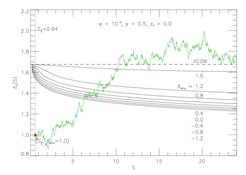
Figure 4: (Colour online) The moving barriers $\delta_{c}(S)$ for different values of $\delta_{\rm env}$ as indicated beside the solid curves. The dashed line is the constant $\delta_{c}$ for spherical collapse in the $\Lambda$CDM model. The vertical dotted line represents $S=S_{\xi}=\sigma^{2}_{8}=0.64$, which gives the length scale used to define environment. Also plotted is the trajectory of a Brownian random walk which starts at $(S_{\xi},\delta_{\rm env}=1.0)$ (the triangle). Note that the first crossing happens earlier in the chameleon models because the barrier is lower.

3.5.2 Conditional First Crossing of a Moving Barrier

The unconditional first crossing distribution, which relates directly to the halo mass function in the $\Lambda$CDM model, is not particularly useful in the chameleon model. This is because spherical overdensities in different environments will follow different evolution paths. If it is in the environment specified by $\left(\delta_{\rm env},S_{\xi}\right)$, then $\left(\delta_{\rm env},S_{\xi}\right)$ should be the starting point of the Brownian motion trajectory. In other words, we actually require the first crossing distribution conditional on the trajectory passing $\delta_{\rm env}$ at $S=S_{\xi}$. Note that in a broader sense the unconditional distribution is a conditional one with $\left(\delta_{\rm env},S_{\xi}\right)=(0,0)$.

Evidently, $\delta_{\rm env}$ has its own distribution: very dense and very empty environments are both quite rare. To quantify this distribution, we need to first define the environment, or equally its smoothing scale $\xi$, which has been chosen to be $8h^{-1}$Mpc above.

The problem then reduces to the calculation of the first crossing probability conditional on the Brownian motion trajectory passing $\delta_{\rm env}$ at $S_{\xi}=\sigma^{2}_{8}$: $f(\delta_{c}(S,\delta_{\rm env}),S~{}|~{}\delta_{\rm env},S_{\xi})$, where we have written explicitly the $\delta_{\rm env}$-dependence of $\delta_{c}$. The numerical algorithm to calculate the conditional first crossing probability is a simple generalisation of the one used above to compute the unconditional first crossing probability (Parfrey et al., 2011) and is not presented in detail here.

Fig. 4 shows the moving barrier $\delta_{c}(S)$ as a function of $S$ for different values of $\delta_{\rm env}$. As an illustration, we have also shown a Brownian motion trajectory which passes $\delta_{\rm env}=1.0$ at $S_{\xi}=\sigma^{2}_{8}=0.64$ (the triangle). Clearly, the larger the value of $\delta_{\rm env}$, the more likely the Brownian motion will hit the barrier at smaller $S$. This is what we see in Fig. 5, which shows the conditional distribution $f(\delta_{c}(S,\delta_{\rm env}),S~{}|~{}\delta_{\rm env},S_{\xi})$ for different values of $\delta_{\rm env}$.

For comparison we also show the corresponding results for the $\Lambda$CDM model using the dashed curves in Fig. 5. Note that the solid curves are always higher than the dashed ones for smaller $S$ and lower for bigger $S$. This is because in the chameleon model the barrier is generally lower and the Brownian motion is likely to cross it for the first time at smaller $S$.

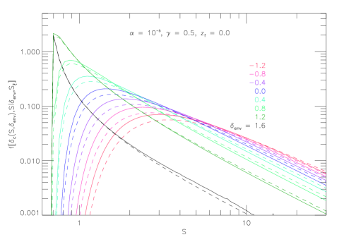
Figure 5: (Colour online) The condition first-crossing distribution for Brownian random walks starting off at $(S_{\xi},\delta_{\rm env})$ in the chameleon (the solid curves) and $\Lambda$CDM models (dashed curves). This depends sensitively on the values of $\delta_{\rm env}$ (indicated above the curves) as explained in the text. Some physical parameters are also shown.

3.5.3 Integrating over the Environment Distribution

To get the final first crossing distribution of the moving barrier, we must integrate over all environments. The distribution of $\delta_{\rm env}$, denoted as $q(\delta_{\rm env},\delta_{\rm sc},S_{\xi})$, in which $\delta_{\rm sc}$ is the critical overdensity for the spherical collapse in the $\Lambda$CDM model, is simply the probability that the Brownian motion passes $\delta_{\rm env}$ at $S_{\xi}$ and never exceeds $\delta_{\rm sc}$ for $S<S_{\xi}$ (because otherwise the environment itself has collapsed already). This has been derived by Bond et al. (1991):

$$q(\delta_{\rm env},\delta_{\rm sc},S_{\xi}) = \frac{1}{\sqrt{2\pi S_{\xi}}}\exp\left[-\frac{\delta^{2}_{\rm env}}{2S_{\xi}}\right]$$ (45)

$$-\frac{1}{\sqrt{2\pi S_{\xi}}}\exp\left[-\frac{\left(\delta_{\rm env}-2\delta_{\rm sc}\right)^{2}}{2S_{\xi}}\right],$$

for $\delta_{\rm env}\leq\delta_{\rm sc}$ and $0$ otherwise.

Then the environment-averaged first crossing distribution will be

$$f_{\rm ave}(S) = \int^{\delta_{\rm sc}}_{-\infty}q\times f(\delta_{c}(S,\delta_{\rm env}),S~{}|~{}\delta_{\rm env},S_{\xi})d\delta_{\rm env}.$$ (46)

In the special case where the barrier is flat, $\delta_{c}(S,\delta_{\rm env})=\delta_{\rm sc}$, $f(\delta_{c}(S,\delta_{\rm env}),S~{}|~{}\delta_{\rm env},S_{\xi})$ is known analytically as

$$f = \frac{\delta_{\rm sc}-\delta_{\rm env}}{\sqrt{2\pi}\left(S-S_{\xi}\right)^{3/2}}\exp\left[-\frac{\left(\delta_{\rm sc}-\delta_{\rm env}\right)^{2}}{2\left(S-S_{\xi}\right)}\right],$$ (47)

and the integration in Eq. (46) can be performed exactly to obtain

$$f_{ave}(S) = \frac{1}{\sqrt{2\pi S}}\frac{\delta_{\rm sc}}{S}\exp\left[-\frac{\delta^{2}_{\rm sc}}{2S}\right],$$ (48)

which is just the unconditional first crossing distribution for a constant barrier $\delta_{\rm sc}$ at $S$. This is as expected, because the collapse does not depend on the environment.

Figure 6: Upper panel: the mass functions for the chameleon (solid curve) and $\Lambda$CDM (dashed curve) models. Some physical parameters are shown in the figure, and others include $\Omega_{m}=0.24$. Lower panel: the fractional differences between the two mass functions (solid curve); the dashed line is identically zero and is shown as a reference.

In general cases with environment-dependent collapse, $f_{\rm ave}(S)$ must be computed numerically. Indeed, in Eq. (46) both $q(\delta_{\rm env},\delta_{\rm sc},S_{\xi})$ and $f(\delta_{c}(S,\delta_{\rm env}),S~{}|~{}\delta_{\rm env},S_{\xi})$ differ from the flat-barrier case. The distribution $f$ has been discussed above (cf. Fig. 5). The distribution $q$ should, in principle, be calculated for the chameleon model numerically, but we choose to use the $\Lambda$CDM result Eq. (45) for the following reasons: recall that $q(\delta_{\rm env},\delta_{\rm sc},S_{\xi})$ is the probability that the Brownian motion starts off at the origin, never hits the constant barrier $\delta_{\rm sc}$ before $S_{\xi}$ and goes through $\delta_{\rm env}$ at $S_{\xi}$. To estimate its difference from the true value in the chameleon model, we replace the $\delta_{\rm sc}$ in Eq. (45) with $\delta_{c}(S_{\xi})$ for the $\delta_{\rm env}$ values in the figures, and find that the change of $q$ is at percent and subpercent level, which is not surprising given that $\delta_{c}(S\leq S_{\xi})$ is very close to $\delta_{\rm sc}$ (cf. Fig. 4) (the approximation will be even better for higher redshift cf. Fig. 3). A better approximation would be to assume $\delta_{c}(S)\approx\delta-\beta S$ where $\beta$ is some constant, but here we do not see the necessity for doing this.

Using Eq. (45), we perform the integral in Eq. (46) using Gaussian quadrature. We checked the accuracy of this method by applying it to the flat-barrier case and find that the agreement with the exact solution is excellent. The halo mass function is related to the averaged first-crossing distribution $f_{\rm ave}(S)$ by

$$\frac{dn}{dM}dM=\frac{\bar{\rho}_{m}}{M}f_{\rm ave}(S)\left|\frac{dS}{dM}\right|dM,$$

and we have plotted in Fig. 6 the function $dn(M,z=0)/dM$ for both the chameleon (solid curves) and the $\Lambda$CDM (dashed curve) models. As can be seen clearly, the fifth force results in more massive halos than in the $\Lambda$CDM model, but in compensation there are fewer low mass halos ($M<10^{12}h^{-1}M_{\bigodot}$) in the chameleon model.

To see the difference more clearly, we have also plotted the fractional difference between the chameleon and $\Lambda$CDM mass functions in the lower panel of Fig. 6. This shows that the increase of $n(M)$ is largest for halos in the mass range $10^{13}<M/\left(h^{-1}M_{\bigodot}\right)<10^{14}$. For high mass halos the fifth force is strongly suppressed and its effect on the mass function is smaller, as expected. Because a larger fraction of the total mass has been assembled in high mass halos, fewer small isolated halos survive the merger and accretion process.

Figure 7: The critical $\Lambda$CDM-linearly-evolved overdensity for spherical collapse at $z_{f}=0$ as a function of the mass enclosed and the environment $\delta_{\rm env}$. The physical parameters $\alpha,\gamma$ are indicated beside each panel. In each panel the solid curves from top to bottom are respectively for $\delta_{\rm env}=1.6,1.2,0.8,0.4,0.0,-0.4,-0.8$ and $-1.2$. The dashed line is the result for $\Lambda$CDM model.

Figure 8: The same as Fig. 8, but for collapsing redshift $z_{f}=1$. In each panel the solid curves from top to bottom are respectively for $\delta_{\rm env}=2.4,1.8,1.2,0.6,0.0,-0.6,-1.2$ and $-1.8$.

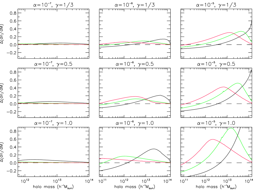
Figure 9: (Colour online) The fractional difference of $dn/dM$ between the chameleon (the scalar field parameters $\alpha$ and $\gamma$ are indicated beside each panel) and $\Lambda$CDM models, at three redshifts $0$ (black curves), $1$ (green curves) and $2$ (red curves). The result for $\Lambda$CDM is plotted as the dashed line for reference.

Note that the effects of the fifth force are suppressed for high mass halos, not only because the halos are efficient at screening that force themselves, but also because they are more likely to reside in dense environments. More explicitly, the probability distribution of $\delta_{\rm env}$ at $S=S_{\xi}$, given that the Brownian motion goes through $\delta\sim\delta_{c}(S)$ at $S$ (where it is about to cross the barrier), is

$$p(\delta_{\rm env}~{}|~{}S,\delta)=\frac{1}{\sqrt{2\pi\frac{S_{\xi}}{S}(S-S_{\xi})}}\exp\left[-\frac{\left(\delta_{\rm env}-\frac{S_{\xi}}{S}\delta\right)^{2}}{2\frac{S_{\xi}}{S}(S-S_{\xi})}\right].$$

For high mass halos, $S$ is close to $S_{\xi}$ and this distribution strongly peaks at $\delta_{\rm env}\sim S_{\xi}\delta/S\sim\delta$. The results, of course, are consistent with our intuitive understanding about the chameleon effect.

4 Applications

The key new concept in our extended excursion set model is the specification of the environment in terms of two parameters $(S_{\xi},\delta_{\rm env})$: the environment determines how spherical collapse in the chameleon model is modified compared to $\Lambda$CDM, and also means that we have to use conditional distribution of the first crossing rather than the unconditional distriubtion, as in the conventional excursion set approach, to compute observables such as the mass function of non-linear structures.

The use of the conditional first-crossing distribution is not new. Mo & White (1996), for example, used it to study the bias between the halo number density and the dark matter density fields in the $\Lambda$CDM model. In the chameleon model, both bias and the mass function must be computed using the conditional first-crossing distribution. In fact, computation of the mass function is more complicated since we need to average over the probability distribution of environments.

The methods introduced here can be used to study, for example, the formation redshift of halos $z_{f}$ and their dependence on the parameters $\alpha$ and $\gamma$ describing the chameleon mechanism, $z_{f}$. The most difficult step in such a calculation is the computation of the moving and environment dependent barrier $\delta_{c}(S,\delta_{\rm env})$. Nevertheless, the computations are very much faster that $N$-body simulations and so we can explore large regions of parameter space rapidly.

Table 1: The parameters $\alpha$ and $\beta$ for the 9 chameleon models studied in this section. The $\Lambda$CDM paradigm corresponds to $\alpha=\beta=0$. We assume $\Omega_{m}=0.24$ and $\Omega_{\Lambda}=0.76$.

$\lg(\alpha)$	$-7$	$-7$	$-7$	$-6$	$-6$	$-6$	$-5$	$-5$	$-5$
$\beta$	$1/3$	$1/2$	$1$	$1/3$	$1/2$	$1$	$1/3$	$1/2$	$1/1$

Let us consider the mass functions of the chameleon models with model parameters as specified in Table 1. Fig. 7 shows the critical density for a spherical overdensity to collapse at $z_{f}=0$ as a function of the enclosed mass $M$ and environment $\delta_{\rm env}$. As expected, the collapse threshold is lower in all chameleon models because the fifth force, however weak, is always attractive and boosts the collapse. For smaller $\alpha$ (left column, $\alpha=10^{-7}$), the difference from the $\Lambda$CDM prediction is small, especially for the largest overdensities because the fifth force is more strongly suppressed in these systems, as discussed in the previous section. On the other hand, for large $\alpha$ (middle and right columns, $\alpha=10^{-6}$ and $10^{-5}$), the deviation from $\Lambda$CDM is much larger, even for the largest overdensities. Increasing $\gamma$ will strengthen the fifth force and therefore also lower the collapse threshold.

Fig. 8 is equivalent to Fig. 7, but for spherical overdensities which collapse at $z_{f}=1$. Because the matter density is higher at higher redshift, the fifth force is more strongly suppressed and hence the deviation from $\Lambda$CDM is smaller.

Finally, we have plotted the effect of a chameleon-type fifth force on the dark matter halo mass functions in Fig. 9. For clarity Fig. 9 shows the fractional change of the quantity $dn/dM$, where $n(M)$ is the halo mass function, with respect to the $\Lambda$CDM prediction, at three redshifts $z=0,1,2$ respectively. For $\alpha=10^{-7}$, the fifth force is strongly suppressed and the fractional change of $dn/dM$ is less than $10$%, even for $\gamma=1$ and $z=0$.

For $\alpha=10^{-6}$, the fifth force is less suppressed and the fractional change of $dn/dM$ at $z=0$ could be up to $\sim 15$% (for $\gamma=1/3$) or even $\sim 40$% (for $\gamma=1$), showing interesting and potentially observable effects. The deviation at early times is mainly restricted to lower mass halos. At later times, massive halos also start to feel the fifth force, and a deviation is seen at higher halo masses. With $\alpha=10^{-5}$, the qualitative features mentioned above all remain, but the deviation from $\Lambda$CDM is much stronger, up to $\sim 60$% for $\gamma=1/3$ and more than $100$% for $\gamma=1$ at $z=0$.

Figs. 7-9 show that some choices of parameters can lead to large deviations in the abundances of non-linear objects compared to the $\Lambda$CDM model. The tightest constraints on the parameters $\alpha$ and $\beta$ would probably come from number counts and number densities of well characterised galaxy cluster samples intermediate redshifts, $z<1$. Such samples are becoming available from combined Sunayev-Zeldovich/X-ray measurements from Planck (Planck collaboration, 2011) and SPT (Carlstrom et al., 2011). A detailed comparison of observations with our model is beyond the scope of this paper.

One question one might ask is if the chameleon model could be used to produce more halos at very early times, say $z>6$, which might ease problems in reionizing the intergalactic medium at early times. It has been argued (Hellwing et al. (2010)) that a fifth force might boost hierarchical structure formation leading to enhanced production of UV photons at early times. Unfortunately, the chameleon-type fifth force is strongly suppressed at earlier times. Fig. 9 shows this up to $z=2$, and for $z>6$ the deviation from $\Lambda$CDM is even smaller.

5 Summary and Conclusions

To summarise, in this paper we have presented an extension of the standard excursion set theory so that it can be used to study structure-formation scenarios which are environmentally dependent. Our method separates the calculation into two steps:

1. compute the collapse of the spherical overdensity in a given environment;

2. compute the probability that the spherical overdensity is located in the specified environment, and average over the distribution of environments.

For (i) we have proposed a simplified model, which is a generalisation of the usual spherical collapse model to the case in which the overdensity evolves inside an evolving environment. For (ii) we have derived an approximation to the environment distribution, and shown how to compute the averaged first-crossing distribution, which is closely related to the halo mass functions.

As a working example, we have applied the method to the chameleon model. Our numerical results agree with how we expect the chameleon effect to behave as a function of the model parameters. We have concentrated here on the collapse redshift and mass functions of virialized objects. These predictions could be used in conjunction with forthcoming data to set constraints on the model parameters.

As in the standard excursion set theory for the cold dark matter model, it is straightforward to generalise the excursion set approach to compute other observables, for example the formation of voids (Sheth & van de Weygaert, 2004) and the merger history of halos (Lacey & Cole, 1993). In conjunction with the halo model, our method can be used to predict the non-linear matter power spectrum as well.

Structure formation scenarios with strong environment dependence have become more and more popular recently. Newtonian gravity has been tested to high precision in our local environment, but deviations may be significant on cosmological scales, perhaps as a result of a chameleon-like mechanism. The methods presented here offer a faster alternative to $N$-body simulations, enabling a much wider range of models to be confronted with observations. Meanwhile, the analytic formulae presented here enable a clear track of the underlying physics, such as in which ways the chameleon effect modifies the structure formation. We hope that these methods will contribute towards a better understanding of the nature of dark energy.

References

- Bond et al. (1991) Bond J. R., Cole S., Efstathiou G., Kaiser N., 1991, ApJ, 379, 440
- Brax et al. (2010) Brax P., van de Bruck C., Davis A. C., Shaw D. J., 2010, PRD, 82, 063519
- Brax et al. (2011) Brax P., van de Bruck C., Davis A. C., Li B., Shaw D. J., 2011, PRD, in press
- Carlberg & Couchman (1988) Carlberg R. G., Couchman H. M. P., 1988, ApJ, 340, 47
- Carlstrom et al. (2011) Carlstrom J. E., et al. 2011, Publ. Astron. Soc. Pac., 123, 568
- Carroll et al. (2005) Carroll S. M., de Felice A., Duvvuri V., Easson D. A., Trodden M., Turner M. S., 2005, PRD, 71, 063513
- Cole & Kaiser (1988) Cole S., Kaiser N., 1988, MNRAS, 233, 637
- Cole & Kaiser (1989) Cole S., Kaiser N., 1989, MNRAS, 237, 1127
- Copeland et al. (2006) Copeland E. J., Sami M., Tsujikawa S., 2006, IJMPD, 15, 1753
- Davis et al. (2011) Davis A. C., Li B., Mota D. F., Winther H. A., 2011, arXiv:1108.3082 [astro-ph.CO]
- Efstathiou & Rees (1988) Efstathiou G., Rees M., MNRAS, 230, 5
- Efstathiou et al. (1988) Efstathiou G., Frenk C. S., White S. D. M., Davis M., 1988, MNRAS, 235, 715
- Hellwing et al. (2010) Hellwing W. A., Knollmann S. R., Knebe A., 2010, MNRAS, 408, L104
- Hinterbichler & Khoury (2010) Hinterbichler K., Khoury J., 2010, PRL, 104, 231301
- Hu & Sawicki (2007) Hu W., Sawicki I., 2007, PRD, 76, 064004
- Khoury & Weltman (2004) Khoury J., Weltman A., 2004, PRD, 69, 044026
- Komatsu et al. (2011) Komatsu E., Smith K. M., Dunkley J., Bennett C. L., Gold B., Hinshaw G., et al., 2011, ApJS, 192, 18
- Lacey & Cole (1993) Lacey C., Cole S., 1993, MNRAS, 262, 627
- Li (2011) Li B., 2011, MNRAS, 411, 2615
- Li & Barrow (2007) Li B., Barrow J. D., 2007, PRD, 75, 084010
- Li & Barrow (2011) Li B., Barrow J. D., 2011, PRD, 83, 024007
- Li, Mota & Barrow (2011) Li B., Mota D. F., Barrow J. D., 2011, ApJ, 728, 109
- Li & Zhao (2009) Li B., Zhao H., 2009, PRD, 80, 044027
- Li & Zhao (2010) Li B., Zhao H., 2010, PRD, 81, 104047
- Li et al. (2011) Li B., Zhao G., Teyssier R., Koyama K., 2011, arXiv:1110.1379 [astro-ph.CO]
- Martino et al. (2009) Martino M., Stabenau H. F., Sheth, R. K., 2009, PRD, 79, 084013
- Mo & White (1996) Mo H. J., White S. D. M., 1996, MNRAS, 282, 347
- Mota & Shaw (2007) Mota D. F., Shaw, D. J., 2007, PRD, 75, 063501
- Narayan & White (1987) Narayan R., White S. D. M., 1987, MNRAS, 231, 97
- Oyaizu (2008) Oyaizu H., 2008, PRD, 78, 123523
- Oyaizu et al. (2008) Oyaizu H., Lima M., Hu W., 2008, PRD, 78, 123524
- Parfrey et al. (2011) Parfrey K., Hui L., Sheth, R. K., 2011, PRD, 83, 063511
- Perlmutter et al. (1999) Perlmutter S. et. al., 1999, ApJ, 517, 565
- Planck collaboration (2011) Planck Collaboration; Ade P. A. R., et. al., 2011, A & A, accepted [URL: http://www.rss.esa.int/Planck.]
- Riess et al. (1998) Riess A. G. et. al., 1998, Astron. J., 116, 1009
- Schaeffer & Silk (1988) Schaeffer R., Silk J., 1988, ApJ, 292, 319
- Schmidt et al. (2009) Schmidt F., Lima M., Oyaizu H., Hu W., 2009, PRD, 79, 083518
- Sheth (1998) Sheth R. K., 1998, MNRAS, 300, 1057
- Sheth & Tormen (2002) Sheth R. K., Tormen G., 2002, MNRAS, 329, 61
- Sheth & van de Weygaert (2004) Sheth R. K., van de Weygaert R., 2004, MNRAS, 350, 517
- Valageas (2009) Valageas P., 2009, A & A, 508, 93
- Wang et al. (2000) Wang L., Caldwell R. R., Ostriker J. P., Steinhardt P. J., 2000, ApJ, 530, 17
- Will (2006) Will C. M., ”The Confrontation between General Relativity and Experiment”, Living Rev. Relativity 9, (2006), 3. URL: http://www.livingreviews.org/lrr-2006-3
- Zentner (2007) Zentner A. R., 2007, IJMPD, 16, 763
- Zhang & Hui (2006) Zhang J., Hui L., 206, ApJ, 641, 641
- Zhao, Li & Koyama (2011a) Zhao G., Li B., Koyama K., 2011, PRD, 83, 044007