The prediction method of similar cycles

Abstract

The concept of degree of similarity ($\eta$) is proposed to quantitatively describe the similarity of a parameter (e.g. the maximum amplitude $R_{\mathrm{max}}$) of a solar cycle relative to a referenced one, and the prediction method of similar cycles is further developed. For two parameters, the solar minimum ($R_{\mathrm{min}}$) and rising rate ($\beta_{\mathrm{a}}$), which can be directly measured a few months after the minimum, a synthesis degree of similarity ($\eta_{\rm s}$) is defined as the weighted-average of the $\eta$ values around $R_{\mathrm{min}}$ and $\beta_{\mathrm{a}}$ with the weights given by the coefficients of determination of $R_{\mathrm{max}}$ with $R_{\mathrm{min}}$ and $\beta_{\rm a}$, respectively. The monthly values of the whole referenced cycle can be predicted by averaging the corresponding values in the most similar cycles with the weights given by the $\eta_{\rm s}$ values. Cycles 14 and 10 are found to be the two most similar cycles of Cycle 24. As an application, Cycle 24 is predicted to peak around January 2013 $\pm$ 8 (months) with a size of about $R_{\mathrm{max}}=84\pm 17$ and to end around September 2019.

1 Introduction

Solar activity prediction is important for both space weather and solar physics. Since solar activity is the driver of various phenomena in the near-Earth environment, knowing the future level of solar activity in advance can reduce some of the hazards for high-tech equipment on which our modern society dependents. Successful predictions could provide some constraints on solar dynamo models (Cameron & Schüssler, 2008; Pesnell, 2008; Wang et al., 2009a; Guo et al., 2010; Du, 2011a).

Various techniques have been used in the past to predict solar activity, of which some were purely statistical and others were related to physics (Kane, 2007; Zhan-leDu et al., 2008; Pesnell, 2008; Messerotti et al., 2009). Geomagnetic precursor methods have attracted more attention due to successes in Cycles 20-22 (Ohl, 1966; Kane, 2007; Du et al., 2009a; Du & Wang, 2011). They are based on a solar dynamo concept that the geomagnetic activity during the declining phase of the preceding cycle or at the minimum provides an approximate measure of the poloidal solar magnetic field that generates the toroidal field for the next cycle (Schatten et al., 1978). Solar dynamo models have recently been attempted, but they are as yet immature to predict the associated solar activity (Dikpati et al., 2006; Tobias et al., 2006; Pesnell, 2008).

A prominent feature in solar activity is the so-called Waldmeier effect, where stronger cycles tend to rise faster (Waldmeier, 1939; Hathaway et al., 2002; Du et al., 2009b). This effect implies that the magnetic energy in a solar cycle has a tendency of stability and that stronger cycles need less time to release their energies (Du, 2006). Correspondingly, the maximum amplitude ($R_{\mathrm{max}}$) of a solar cycle is well correlated with the growth rate of activity in the early phase (Cameron & Schüssler, 2008).

As a new solar cycle is ongoing, its shape can be well described by simple functions containing a few parameters (Elling & Schwentek, 1992; Hathaway et al., 1994; Li, 1999; Volobuev, 2009; Du, 2011b). Before the arrival of the peak of a solar cycle, only two parameters are known: the preceding minimum ($R_{\mathrm{min}}$) and the rising rate ($\beta_{\mathrm{a}}$), defined as the ratio of the increment of the activity ($R_{\mathrm{z}}$) and the elapsed time duration. The two parameters can be taken as indicators for the subsequent amplitude ($R_{\mathrm{max}}$).

Solar cycles that have approximatively the same $R_{\mathrm{max}}$ tend to have similar shapes, and these cycles are therefore called ‘similar cycles’ (Waldmeier, 1936; Gleissberg, 1971; Wang et al., 2002). Gleissberg (1971) used the concept that similar cycles tend to have similar cycle lengths and similar decline times (Gleissberg, 1973) to estimate the epochs of the start and end of Cycle 21 by averaging the cycle lengths and decline times of similar cycles, respectively. Wang & Han (1997) developed the concept of similar cycles and used it to predict $R_{\mathrm{max}}$ (Wang et al., 2009b) and monthly values of $R_{\mathrm{z}}$ (Wang et al., 2002; Miao et al., 2008). The predicted value of $R_{\mathrm{z}}$ for month $i$ is taken as the average of the corresponding values of similar cycles for the same month from the start of the cycles, and the standard deviation of these values is taken as the prediction error for the same month.

The data and parameters used in this study are shown in Section 2. Some of the correlations between these parameters are analyzed in Section 3, and in Section 4, we employ the two parameters of $R_{\mathrm{min}}$ and $\beta_{\mathrm{a}}$ to further develop the concept of a similar cycle and its application in prediction. In Section 4.1, a quantity, the “degree of similarity ($\eta$)”, is proposed to describe the similarity of a parameter in past cycles relative to a referenced one (the predictor for a cycle to be predicted). For two predictors ($R_{\mathrm{min}}$, $\beta_{\mathrm{a}}$), in Section 4.2, a synthesis degree of similarity ($\eta_{\mathrm{s}}$) is defined as the weighted-average of the corresponding $\eta$ values ($\eta_{\mathrm{R}}$, $\eta_{\mathrm{\beta}}$) with the weights given by the coefficients of determination of $R_{\mathrm{max}}$ with $R_{\mathrm{min}}$ and $\beta_{\rm a}$ ($r^{2}_{\rm R}$, $r^{2}_{\rm\beta}$), respectively. Then, the $R_{\mathrm{max}}$ value for the current cycle (24) can be predicted as the weighted-average of the $R_{\mathrm{max}}$ values of the five most similar cycles with the weights given by $\eta_{\mathrm{s}}$. The same technique is used in Section 4.3 for each month from the start of the similar cycles to obtain the monthly values (shape) of Cycle 24. The predictive power of the similar-cycle prediction method is tested on different months from the start of Cycle 24 in Section 4.4. The results are briefly discussed and summarized in Section 5.

2 Data and cycle parameters

The data used in this study are the smoothed monthly mean Zürich relative sunspot numbers ($R_{\mathrm{z}}$) of the more reliable data since Cycle 8 (up to November 2010). Some parameters of the solar cycle are listed in Table 1, where $R_{\rm max}$ and $R_{\rm min}$ are the maximum and minimum amplitudes of a solar cycle, respectively. Here $\beta_{\rm a}$ is the rising rate at $\Delta m$ months entering into the cycle,

$$\beta_{\rm a}=\Delta R_{\rm z}/\Delta m,$$ (1)

where $\Delta R_{\rm z}=R_{\rm z}(\Delta m)-R_{\rm min}$ is the increment of $R_{\rm z}$ from $R_{\rm min}$ in the time interval of $\Delta m$ (months). At the present time, $\Delta m=24$ (months) for the data available in the current cycle (24). $S$ is the skewness of the cycle, a measure of symmetry about its maximum,

$$S=\frac{\sum_{i=1}^{N}(y_{i}-\overline{y})^{3}}{(N-1)\sigma^{3}},$$ (2)

where $y=R_{\rm z}$ is the data series for a solar cycle, $\overline{y}$ is the mean, $N$ the number of data points, and $\sigma$ the standard deviation. Positive (negative) skewness indicates that the distribution is skewed to the right (left), with a longer tail to the right (left) of the maximum.

Table 1: Parameters since cycle $n=8$.

$n$	$R_{\rm min}$	$\beta_{\rm a}(21)$	$\beta_{\rm a}(24)^{\mathrm{e}}$	$R_{\rm max}$	$S$
8	7.3	2.85	3.31	146.9	0.28
9	10.6	1.10	1.25	131.9	0.51
10	3.2	1.24	1.37	98.0	0.14
11	5.2	2.48	2.63	140.3	0.52
12	2.2	1.65	1.73	74.6	0.09
13	5.0	2.32	2.38	87.9	0.35
14	2.7	1.28	1.37	64.2	$-0.09$
15	1.5	1.94	1.95	105.4	0.33
16	5.6	1.29	1.73	78.1	0.02
17	3.5	1.46	1.79	119.2	0.12
18	7.7	2.11	2.47	151.8	0.16
19	3.4	4.07	4.80	201.3	0.30
20	9.6	1.94	2.42	110.6	0.03
21	12.2	2.32	2.68	164.5	0.13
22	12.3	3.88	4.54	158.5	0.16
23	8.0	1.95	2.14	120.8	0.30
24	1.7	0.75	1.03
$\overline{x}^{\mathrm{a}}$	6.3	2.12	2.04	122.1	0.21
$\sigma_{\rm x}^{\mathrm{b}}$	3.5	0.88	0.91	37.4	0.17
$r^{\mathrm{c}}$	0.39	0.36	0.15	0.33	$-0.32$
CL(%)d	86.4	82.7	$<50$	78.4	76.1

• Average for $n=8$-23.

• Standard deviation.

• Correlation coefficient of temporal trend.

• The confidence level (%).

• At the current state.

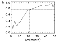
Figure 1: (a) $\beta_{\rm a}$ as a function of $\Delta m$ for Cycles 8-24. The dashed lines indicate $\beta_{\rm a}$ for Cycles 14, 10, 17, 16 and 12. The thick solid line indicates the averages for the data available. (b) Correlation coefficient ($r$) between $R_{\rm max}$ and $\beta_{\rm a}$.

In Table 1, $\overline{x}$ and $\sigma$ are the average and standard deviation of the parameters for Cycles $n=8$-23, respectively, $r$ is the correlation coefficient of the parameter with time (temporal variation), and CL is the confidence level.

It is shown in Table 1 that $R_{\rm min}$, $\beta_{\rm a}$ and $R_{\rm max}$ all show an increasing trend with time ($r>0$) at the confidence level (CL) around 80%, and that $S$ used to be positive ($\overline{S}=0.21$), meaning that the decline time tends to be longer than the rise time for most solar cycles. However, this asymmetry seems to decrease as can be seen from the decreasing temporal trend ($r=-0.32$) in $S$.

The $\beta_{\rm a}$ values for Cycles 8-24 are shown in Fig. 1(a). It is seen in this figure that $\beta_{\rm a}$ varies approximately linearly with $\Delta m$ at the early phase of the cycle (about $\Delta m\leq 26$) and has decreases since then. The correlation coefficient ($r$) between $R_{\rm max}$ and $\beta_{\rm a}$ varies with an increasing trend (Fig. 1b) and $r>0.75$ when $\Delta m\geq 21$. First, we take $\Delta m=21$ (months) as an example to describe the method of similar cycles. Then, this method is applied to $\Delta m=18,19,\cdots,24$ (months) for predicting Cycle 24.

3 Correlation between some parameters

Of the parameters describing the solar cycle, only $R_{\mathrm{min}}$ and $\beta_{\rm a}$ are known before the timing of $R_{\mathrm{max}}$. Therefore, both $R_{\mathrm{min}}$ and $\beta_{\rm a}$ can be taken as indicators for the subsequent $R_{\mathrm{max}}$. Figure 2(a) shows the scatter plot of $R_{\mathrm{max}}$ against $R_{\mathrm{min}}$ with the least-square-fit linear regression equation given by

$$R_{\mathrm{max}}=91.3+4.94R_{\mathrm{min}},\sigma=33.1,$$ (3)

where $\sigma$ is the standard deviation. It is well known that $R_{\mathrm{max}}$ is weakly correlated with the preceding $R_{\mathrm{min}}$ ($r_{\rm R}=0.47$), at the 92.9% confidence level, so that a small $R_{\mathrm{min}}$ tends to be followed by a weak cycle (Hathaway et al., 2002; Li, 2009). However, since this correlation is weak, one can hardly obtain an accurate prediction of $R_{\mathrm{max}}$ by $R_{\mathrm{min}}$ alone (Du & Wang, 2010).

Figure 2: Scatter plots of (a) $R_{\mathrm{max}}$ against $R_{\mathrm{min}}$, (b) $R_{\mathrm{max}}$ against $\beta_{\rm a}$, (c) $S$ against $R_{\mathrm{max}}$, (d) $S$ against $\beta_{\rm a}$.

Figure 2(b) shows the scatter plot of $R_{\mathrm{max}}$ against $\beta_{\mathrm{a}}$. The best linear relationship between them is

$$R_{\mathrm{max}}=54.4+31.98\beta_{\mathrm{a}},\sigma=24.8.$$ (4)

One can see that $R_{\mathrm{max}}$ is well correlated with the rising rate $\beta_{\rm a}$ ($r_{\rm\beta}=0.75$) at the 99.9% confidence level. Therefore, $\beta_{\rm a}$ is a good predictor for the subsequent $R_{\mathrm{max}}$. Substituting the value of $\beta_{\mathrm{a}}$ (0.75) for $\Delta m=21$ into this equation, the peak size of Cycle 24 can be estimated to be $R_{\mathrm{max}}(24)=78.3\pm 24.8$ (triangle).

The scatter plots of $S$ against $R_{\mathrm{max}}$ and $S$ against $\beta_{\rm a}$ are shown in Figs. 2(c) and (d), respectively. The correlation coefficients involved are listed in Table 2.

Table 2: Cross-correlation Coefficients ($r$).

$y$	$x$	$r$	CL
$R_{\rm max}$	$R_{\rm min}$	0.47	92.9%
$R_{\rm max}$	$\beta_{\rm a}$	0.75	99.9%
$S$	$R_{\rm max}$	0.41	88.5%
$S$	$\beta_{\rm a}$	0.24	62.0%
$S$	$R_{\rm min}$	0.10

4 Similar cycles

It should be pointed out in Fig. 2(c) that $S$ is positively correlated with $R_{\mathrm{max}}$ ($r=0.41$), so that similar cycles (with approximatively the same $R_{\mathrm{max}}$) tend to have similar shapes, which is a key point in the concept of similar cycles although $r$ is not high. Because if $S$ were uncorrelated with $R_{\mathrm{max}}$, the concept of similar cycles would not have been used any longer. However, as $R_{\mathrm{max}}$ is unknown in advance, the shape of an upcoming cycle cannot be described directly from the measurement of $R_{\mathrm{max}}$, which is usually estimated by an appropriation technique.

Because $R_{\mathrm{max}}$ has a much higher correlation coefficient with $\beta_{\rm a}$ ($r=0.75$) than with $R_{\mathrm{min}}$ ($r=0.47$) and the correlation coefficient of $S$ with $\beta_{\rm a}$ ($r=0.24$) is slightly higher than that of $S$ with $R_{\mathrm{min}}$ ($r=0.10$), $\beta_{\rm a}$ is a much better predictor for $R_{\mathrm{max}}$ than $R_{\mathrm{min}}$. However, the two predictors of $\beta_{\rm a}$ and $R_{\mathrm{min}}$ are expected to provide useful information (size and asymmetry) on the subsequent cycle, because both of them can be directly measured a few months after the minimum.

4.1 Degree of similarity

For a parameter $x=\{x_{i},i=1,2,\cdots,m\}$, the probability density of the normalized deviation,

$$E_{i}=\frac{\Delta x_{i}}{\sigma_{\rm{x}}}=\frac{x_{i}-\overline{x}}{\sigma_{\rm{x}}},$$ (5)

approximately satisfies a normal distribution (Fig. 3a),

$$\rho(E_{i})=\frac{1}{\sqrt{2\pi}}e^{-E_{i}^{2}/2},$$ (6)

where $\overline{x}$ and $\sigma_{\rm{x}}$ are the mean and standard deviation, respectively (Table 1). The probability that $\Delta x_{i}$ falls in the range [$\Delta x_{\rm{r}}$, $\Delta x_{\rm{n}}$] is

$$\Delta P(n)=\frac{1}{\sqrt{2\pi}}\int_{E_{\rm{r}}}^{E_{\rm{n}}}e^{-t^{2}/2}dt,$$ (7)

where $x_{\rm{r}}$ is a referenced value (a predictor for Cycle $n_{\rm{r}}=24$) and $x_{\rm{n}}$ the value in the past cycle ($n$).

Figure 3: (a) Gaussian distribution. (b) $R_{\mathrm{min}}$ (solid) and $\eta_{\mathrm{R}}$ (dashed). (c) $\beta_{\mathrm{a}}$ (solid) and $\eta_{\mathrm{\beta}}$ (dashed). The numbers indicate the similar cycles and their orders in brackets.

A small value of $|\Delta P(n)|$ indicates that $x_{\rm{n}}(=\overline{x}+\Delta x_{\rm{n}})$ is close to $x_{\rm{r}}(=\overline{x}+\Delta x_{\rm{r}})$, in which case Cycle $n$ is called a similar cycle of $n_{\rm{r}}$ around $x_{\rm{r}}$. The smaller the $|\Delta P(n)|$ is, the more similar the two parameters are. Because $0\leq|\Delta P(n)|\leq 1$ for either $x_{\rm{r}}\geq x_{\rm{n}}$ or $x_{\rm{r}}<x_{\rm{n}}$, we define $1-|\Delta P(n)|$ as a measure to describe the “degree of similarity” around $x_{\rm{r}}$,

$$\eta(n)=1-\frac{1}{\sqrt{2\pi}}\left|\int_{E_{\rm{r}}}^{E_{\rm{n}}}e^{-t^{2}/2}dt\right|.$$ (8)

If $\eta(n)=1$, the two parameters are identical, $x_{\rm{n}}=x_{\rm{r}}$ (100% similarity); if $\eta(n)=0$, there is no similarity between them. In application, some (five in this study) of the largest values of $\eta(n)$ are selected and their cycles are called the similar cycles of $n_{\rm{r}}$ around $x_{\rm{r}}$.

4.2 Similar cycles used in predicting $R_{\mathrm{max}}$

Figure 3(b) shows the values of $R_{\mathrm{min}}$ (solid) for Cycles $n=8$-23, the referenced one ($R_{\mathrm{min}}(24)=1.7$, triangle) for Cycle $n_{\rm{r}}=24$, and the values of $\eta$ ($\eta_{\mathrm{R}}$, dashed) around $R_{\mathrm{min}}(24)$. The five biggest values of $\eta_{\mathrm{R}}$ (asterisks) are in Cycles $n_{\mathrm{R}}=15,12,14,10$ and 19 (in that order), which are called the similar cycles of Cycle 24 around $R_{\mathrm{min}}$.

Figure 3(c) shows the values of $\beta_{\mathrm{a}}$ (solid), the referenced one ($\beta_{\mathrm{a}}(24)=0.75$, triangle), and the values of $\eta$ ($\eta_{\mathrm{\beta}}$, dashed) around $\beta_{\mathrm{a}}(24)$. The five biggest values of $\eta_{\mathrm{\beta}}$ (asterisks) are in Cycles $n_{\mathrm{\beta}}=9,10,14,16$ and 17 (in that order), which are called the similar cycles of Cycle 24 around $\beta_{\mathrm{a}}$. These similar cycles ($n_{\mathrm{\beta}}$) are partly different from the above ones around $R_{\mathrm{min}}$ ($n_{\mathrm{R}}$). Since the correlation coefficient of $R_{\mathrm{max}}$ with $\beta_{\mathrm{a}}$ ($r_{\rm{\beta}}=0.75$) is much higher than that ($r_{\rm{R}}=0.47$) of $R_{\mathrm{max}}$ with $R_{\mathrm{min}}$, $n_{\mathrm{\beta}}$ should be more reliable than $n_{\mathrm{R}}$ for describing the information of Cycle $n_{\mathrm{r}}$.

From $\eta_{\rm{R}}$ and $\eta_{\mathrm{\beta}}$, a synthesis degree of similarity around both $R_{\mathrm{min}}$ and $\beta_{\mathrm{a}}$ can be defined as

$$\eta_{\rm{s}}(n)=\frac{\eta_{\mathrm{R}}(n)r_{\rm{R}}^{2}+\eta_{\mathrm{\beta}}(n)r_{\rm{\beta}}^{2}}{r_{\rm{R}}^{2}+r_{\rm{\beta}}^{2}},$$ (9)

here the weights are taken as the coefficients of determination, $W_{\rm{R}}=r^{2}_{\rm{R}}$ and $W_{\rm{\beta}}=r^{2}_{\rm{\beta}}$ for $R_{\mathrm{min}}$ and $\beta_{\mathrm{a}}$, respectively. The reason for such a selection is that about $r^{2}_{\rm{R}}$ ($r^{2}_{\rm{\beta}}$) of the variations in $R_{\mathrm{max}}$ can be explained by the correlation of $R_{\mathrm{max}}$ with $R_{\mathrm{min}}$ ($\beta_{\mathrm{a}}$).

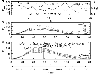
Figure 4: (a) $R_{\mathrm{max}}$ (solid) and $\eta_{\rm{s}}$ (dashed). (b) The values of $R_{\mathrm{z}}$ for similar cycles $n_{s}=14,10,17,16$ and 12. (c) The predicted monthly values of $R_{\mathrm{z}}$ for Cycle 24 with error bars.

Figure 4(a) shows the values of $R_{\mathrm{max}}$ (solid) and $\eta_{\rm{s}}$ (dashed). The five biggest values of $\eta_{\rm{s}}$ (asterisks) are in Cycles $n_{\rm{s}}=14,10,17,16$ and 12 (in that order), which are called the similar cycles of Cycle 24 around both $R_{\mathrm{min}}$ and $\beta_{\mathrm{a}}$. From these values, the peak size of Cycle 24 can be predicted as the weighted-average of those of the similar cycles,

$$\begin{array}[]{rcl}R_{\mathrm{max}}(24)&=&\frac{\sum_{i=1}^{5}R_{\mathrm{max}}(n_{\rm{s}}(i))W(i)}{\sum_{i=1}^{5}W(i)},\\ W(i)&=&\eta_{\rm{s}}(n_{\rm{s}}(i)),\\ \end{array}$$ (10)

where the weights $W(i)$ are taken as the (synthesis) degrees of similarity $\eta_{\rm{s}}(n_{\rm{s}}(i))$. The more similar a cycle is to $n_{\rm{r}}$, the more its weight it should be included. The standard deviation is correspondingly defined as

$$\sigma_{\mathrm{max}}(24)=\sqrt{\frac{\sum_{i=1}^{5}[R_{\mathrm{max}}(n_{\rm{s}}(i))-R_{\mathrm{max}}(24)]^{2}W(i)}{\sum_{i=1}^{5}W(i)}}.$$ (11)

According to the above equations, the peak size of Cycle 24 is predicted to be $R_{\mathrm{max}}(24)=86.8\pm 19.6$ (triangle).

4.3 Similar cycles used in predicting monthly values

Now, we use the above technique to predict the monthly values (shape) of Cycle 24. Figure 4(b) shows the monthly values of $R_{\mathrm{z}}$ for the similar cycles ($n_{\rm{s}}$) from the starting points of the cycles. The $R_{\mathrm{z}}$ value of the $t^{th}$ month in Cycle 24 is predicted as the weighted-average of the corresponding $R_{\mathrm{z}}$ values for the same month in the similar cycles,

$$\overline{R}_{\mathrm{z}}(t)=\frac{\sum_{i=1}^{5}R_{\mathrm{z}}(t,n_{\rm{s}}(i))W(i)}{\sum_{i=1}^{5}W(i)}.$$ (12)

Its standard deviation is

$$\sigma_{\mathrm{z}}(t)=\sqrt{\frac{\sum_{i=1}^{5}(R_{\mathrm{z}}(t,n_{\rm{s}}(i))-\overline{R}_{\mathrm{z}}(t))^{2}W(i)}{\sum_{i=1}^{5}W(i)}}.$$ (13)

The results since November 2008 are shown in Fig. 4(c). From these results, we can obtain the maximum value (83.0), the standard deviation (16.7), the rise time ($T_{\mathrm{a}}=58$ months), and the cycle length (130 months). Cycle 24 is therefore predicted to peak around September 2013 with a size of about $R_{\mathrm{max}}=83.0\pm 16.7$, and to end around September 2019. This size is near that (86.8) in section 4.2 and that (78.3) in Section 3. It should be pointed out in Fig. 4(c) that the shape near the peak is rather flat. Besides the highest peak (83.0) in September 2013, there are two weak peaks preceding it: the first is around June 2012 (81.1) and the second is around January 2013 (80.1). If this result is true, it implies that Cycle 24 will have multiple peaks with the last peak being higher. On average, Cycle 24 may probably peak around January 2013 $\pm 8$ (months).

4.4 Prediction results at $\Delta m$ = 18-24 months

Since $\beta_{\mathrm{a}}$ is a temporal variable of $\Delta m$, the result derived from $\beta_{\mathrm{a}}$ may depend on $\Delta m$, similar to the prediction by a simple function to describe the shape of the solar cycle (Hathaway et al., 1994; Du, 2011b). In this section, we apply the above technique to the current state ($\Delta m=24$), as shown in Fig. 5. The similar cycles at $\Delta m=24$ ($n_{\rm{s}}=$14, 10, 12, 17 and 15) are slightly different from those at $\Delta m=21$ ($n_{\rm{s}}=$14, 10, 17, 16 and 12) in Fig. 4. In Fig. 5(a), the peak size of Cycle 24 is predicted to be $R_{\mathrm{max}}(24)=91.6\pm 20.1$ (triangle) based on the $R_{\mathrm{max}}$ values of the similar cycles, slightly higher than that ($R_{\mathrm{max}}(24)=86.8\pm 19.6$) in Fig. 4(a).

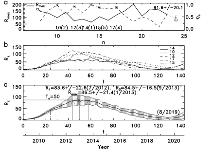
Figure 5: Similar to Fig. 4 but using the $\beta_{\mathrm{a}}$ values at $\Delta m=24$ (month). (a) $R_{\mathrm{max}}$ (solid) and $\eta_{\rm{s}}$ (dashed). (b) The values of $R_{\mathrm{z}}$ for similar cycles $n_{\rm{s}}=14,10,12,17$ and 15. (c) The predicted monthly values of $R_{\mathrm{z}}$ for Cycle 24 with error bars.

In Fig. 5(c), the highest peak is $R_{\mathrm{max}}=86.5\pm 21.4$ in January 2013 (from the predicted monthly $R_{\mathrm{z}}$ in Cycle 24), which is near the second peak in Fig. 4(c). In addition, there are two shoulders: one in July 2012 (83.8) and another in September 2013 (84.5). The former is near the first peak (June 2012) and the latter is just the third peak (September 2013) in Fig. 4(c).

Table 3: Prediction Results for $\Delta m=18,19,\cdots,24$ (months).

$\Delta m$	$\beta_{\rm a}$	$n_{\rm s}$	$R_{\rm max}$(1st peak)	$R_{\rm max}$(2nd peak)	$R_{\rm max}$(3rd peak)	ending
18	0.77	10,17,14,16,15	85.9$\pm$20.5(6/2012)	89.4$\pm$19.2(12/2012)	86.4$\pm$15.8(8/2013)	2/2019
19	0.77	10,17,14,16,12	81.8$\pm$22.7(6/2012)	80.7$\pm$20.6(1/2013)	83.5$\pm$16.8(9/2013)	9/2019
20	0.75	10,14,17,16,12	81.4$\pm$22.6(6/2012)	80.4$\pm$20.6(1/2013)	83.2$\pm$16.7(9/2013)	9/2019
21	0.75	14,10,17,16,12	81.1$\pm$22.6(6/2012)	80.1$\pm$20.5(1/2013)	83.0$\pm$16.7(9/2013)	9/2019
22	0.81	14,10,17,12,16	81.0$\pm$22.5(6/2012)	80.0$\pm$20.5(1/2013)	82.9$\pm$16.7(9/2013)	9/2019
23	0.93	14,10,12,17,16	80.9$\pm$22.5(6/2012)	79.9$\pm$20.5(1/2013)	82.8$\pm$16.7(9/2013)	9/2019
24	1.03	14,10,12,17,15	83.6$\pm$22.6(7/2012)	86.5$\pm$21.4(1/2013)	84.5$\pm$16.5(9/2013)	8/2019
$\overline{x}$			82.2$\pm$22.3(6/2012)	82.4$\pm$20.5(1/2013)	83.8$\pm$16.6(9/2013)	9/2019

Using the same technique, we tested the predictive power of this method at $\Delta m$ = 18 - 24 month. The results are listed in Table 3, where the third column indicates the similar cycles for a given $\Delta m$ (first column); the fourth - sixth columns correspond to the first - third peaks, respectively; and the last column is the ending time of Cycle 24. The last row shows the relevant averages. It is seen in this table that there are not significant differences in the results as the cycle progresses although the similar cycles may have a small difference ($n_{\rm s}$) for different $\Delta m$. The three peaks for different $\Delta m$ are near each other either in size or in date. If the maximum average size and the middle date is taken as those for the peak of the cycle, Cycle 24 is predicted to peak around January 2013 $\pm$ 8 (month) with a size of about $R_{\rm max}=84\pm 17$.

5 Discussions and Conclusions

A concept, the degree of similarity ($\eta$), is proposed to quantitatively describe the similarity of a parameter of a solar cycle relative to a referenced one, and the prediction method of similar cycles is further developed. The degrees of similarity are used as the weights in the weighted-average of the values of a parameter in the similar cycles so as to obtain a predicted one in the referenced cycle, where we have considered the fact that more weights should be paid to the cycles that are more similar to the referenced one.

In this study, we used two predictors, the preceding minimum ($R_{\mathrm{min}}$) and rising rate ($\beta_{\mathrm{a}}$), to define a synthesis degree of similarity ($\eta_{\rm s}$) by averaging the corresponding $\eta$ values with the weights given by the coefficients of determination of $R_{\mathrm{max}}$ with $R_{\mathrm{min}}$ and $\beta_{\rm a}$, respectively. From this method, Cycle 24 is predicted to peak around January 2013 $\pm$ 8 (months) with a size of about $R_{\rm max}=84\pm 17$ and to end around September 2019. This result is slightly lower than that ($100.2\pm 7.5$) predicted by Wang et al. (2009b) based on their similar-cycle method. It is near $80\pm 30$ (Schatten, 2005), $\sim 80$ (Kitiashvili & Kosovichev, 2008), and $\sim 85$ (Jiang et al., 2007) based on polar field or solar dynamo models, but much lower than $\sim 167$ (Dikpati et al., 2006) based on a modified flux-transport dynamo model.

It should be pointed out from Section 4.2 that (i) considering a single parameter $R_{\mathrm{min}}$, the most similar cycle (to Cycle 24) is $n=15$ since $R_{\mathrm{min}}(15)=1.5$ is close to $R_{\mathrm{min}}(24)=1.7$; (ii) considering another single parameter $\beta_{\mathrm{a}}$, the most similar cycle is $n=9$ as $\beta_{\mathrm{a}}(9)=1.10$ is close to $\beta_{\mathrm{a}}(24)=0.75$; and (iii) considering both parameters $R_{\mathrm{min}}$ and $\beta_{\mathrm{a}}$, the most similar cycle is $n=14$. In this study, the similar cycles are selected from two parameters ($R_{\mathrm{min}}$, $\beta_{\mathrm{a}}$) to avoid an accidental error caused by a single parameter. In terms of the synthesis degree of similarity ($\eta_{\rm s}$), Cycle 15 is not a similar cycle since $\beta_{\mathrm{a}}(15)=1.94$ is not so near to $\beta_{\mathrm{a}}(24)$, although $R_{\mathrm{min}}(15)$ is close to $R_{\mathrm{min}}(24)$, and Cycle 9 is not a similar cycle as $R_{\mathrm{min}}(9)=10.6$ is far from $R_{\mathrm{min}}(24)$ although $\beta_{\mathrm{a}}(9)$ is close to $\beta_{\mathrm{a}}(24)$. Therefore, the most similar cycle ($n=14$) is that with maximum $\eta_{\rm s}$ which is the synthesis effect of both $R_{\mathrm{min}}(14)=2.7$ and $\beta_{\mathrm{a}}(14)=1.28$, although Cycle 14 is not the most similar cycle with either $R_{\mathrm{min}}$ or $\beta_{\mathrm{a}}$ alone. Because $\beta_{\mathrm{a}}$ varies with the progression ($\Delta m$) of the cycle, the results from both $R_{\mathrm{min}}$ and $\beta_{\mathrm{a}}$ may have a slight differences (Table 3).

Near the time of a solar minimum, geomagnetic activity is a much better indicator for the ensuing maximum amplitude ($R_{\mathrm{max}}$) of the solar cycle (Ohl, 1966) than the solar minimum ($R_{\mathrm{min}}$). This study shows that the rising rate ($\beta_{\mathrm{a}}$) at the early phase of a solar cycle is also a good indicator for the subsequent $R_{\mathrm{max}}$. This parameter has the advantage that it only needs the $R_{\mathrm{z}}$ series itself. It reflects the initial physical process of solar magnetic activities.

Similar cycles are usually defined as those whose values of $R_{\mathrm{max}}$ (or other parameters) satisfy a given condition (Gleissberg, 1971; Wang & Han, 1997; Wang et al., 2002, 2009b; Miao et al., 2008),

$$|R_{\mathrm{max}}-R_{\mathrm{max}}(n_{\rm r})|\leq\Delta,$$ (14)

where $R_{\mathrm{max}}(n_{\rm r})$ is the referenced value and $\Delta$ is a given limit (e.g., 10 or 20). By averaging the values of a parameter (rise time, decline time or monthly $R_{\mathrm{z}}$ and so on) in these cycles, the corresponding one in the predicted cycle could be obtained. This technique has considered the cycles that have similar $R_{\mathrm{max}}$ to $R_{\mathrm{max}}(n_{\rm r})$. However, how close these cycles are to the referenced one has not been considered, as a simple averaging method ($W(i)=1$) was used in this technique. Besides, $R_{\mathrm{max}}(n_{\rm r})$ is usually unknown, so it also needs to be predicted. The error in $R_{\mathrm{max}}(n_{\rm r})$ may probably propagate into the other parameters that are derived from it. In contrast, this study used the two directly measured parameters ($R_{\mathrm{min}}$, $\beta_{\rm{a}}$) to derive all the information of a cycle to be predicted (24).

The central idea of a similar cycle is that solar cycles with approximatively the same $R_{\mathrm{max}}$ tend to have similar shapes, which is empirical and has not been studied physically as far as we know. It is shown in Fig. 2(c) that $S$ is weakly correlated with $R_{\mathrm{max}}$ ($r=0.41$), which is a key point in the concept of similar cycles. Under this relationship, we can use the concept that solar cycles with approximate $R_{\mathrm{max}}$ might have similar rise times, cycle lengths and cycle shapes, so we can estimate it in the referenced cycle by averaging the corresponding values in similar cycles. However, since $R_{\mathrm{max}}$ is unknown in advance, the shape of an upcoming cycle cannot be estimated directly from $R_{\mathrm{max}}$. In this study, we used both the rising rate ($\beta_{\mathrm{a}}$) and solar minimum ($R_{\mathrm{min}}$) to select the similar cycles, which is based on the correlations of $R_{\mathrm{max}}$ with both $\beta_{\mathrm{a}}$ ($r_{\mathrm{\beta}}\sim 0.75$) and $R_{\mathrm{min}}$ ($r_{\mathrm{R}}=0.47$). If one uses other parameters (e.g., the preceding decline time) to find some similar cycles, the correlations between $R_{\mathrm{max}}$ and these parameters are also needed (even if they are not strong).

One advantage of the similar-cycle method is that it does not involve the details of a physical process. The actual physical process may be rather complicated; its dynamical mechanism is not very clear at present and may not be described by a simple linear or non-linear relationship. Whatever the process is, a similar process may likely occur if the levels of activity are similar, which is what the similar-cycle method can and wants to do. This is similar to treating the complex process as a piecewise function.

The main points in this study can be summarized as follows.

1. A concept, the degree of similarity ($\eta$), is proposed to quantitatively describe the similarity about a parameter for a solar cycle relative to a referenced one.

2. For two parameters, the preceding minimum ($R_{\mathrm{min}}$) and rising rate ($\beta_{\mathrm{a}}$), a synthesis degree of similarity ($\eta_{\rm s}$) is defined as the weighted-average of the corresponding ones with the weights given by the coefficients of determination of $R_{\mathrm{max}}$ with $R_{\mathrm{min}}$ and $\beta_{\rm a}$, respectively.

3. The prediction method of similar cycles is further developed with the weights given by the (synthesis) degrees of similarity.

4. As an application of this method, Cycle 24 is predicted to peak around January 2013 $\pm$ 8 (months) with a size of about $R_{\mathrm{max}}=84\pm 17$ and to end around September 2019.

References

- Cameron & Schüssler (2008) Cameron, R., & Schüssler, M. 2008, ApJ, 685, 1291
- Dikpati et al. (2006) Dikpati, M., de Toma, G., & Gilman, P. A. 2006, Geophys. Res. Lett., 33, L05102
- Du (2006) Du, Z. L. 2006, AJ, 132, 1485
- Du (2011a) Du, Z. L. 2011a, Sol. Phys., 270, 407
- Du (2011b) Du, Z. L. 2011b, Sol. Phys., DOI: 10.1007/s11207-011-9849-8
- Du & Wang (2010) Du, Z. L., & Wang, H. N. 2010, Research in Astron. Astrophys. (RAA), 10, 950
- Du & Wang (2011) Du, Z. L., & Wang, H. N. 2011, Sci. China, Phy. Mech. Astron., 54, 172
- Du et al. (2009a) Du, Z. L., Li, R., & Wang, H. N. 2009a, AJ, 138, 1998
- Du et al. (2009b) Du, Z. L., Wang, H. N. & Zhang, L. Y. 2009b, Sol. Phys., 255, 179
- Elling & Schwentek (1992) Elling, W., & Schwentek, H. 1992, Sol. Phys., 137, 155
- Gleissberg (1971) Gleissberg, W. 1971, Sol. Phys., 21, 240
- Gleissberg (1973) Gleissberg, W. 1973, Sol. Phys., 30, 539
- Guo et al. (2010) Guo, J., Zhang, H. Q., Chumak, O. V., & Lin, J. B. 2010, MNRAS, 405, 111
- Hathaway et al. (2002) Hathaway, D. H., Wilson, R. M., & Reichmann, E. J. 2002, Sol. Phys., 211, 357
- Hathaway et al. (1994) Hathaway, D. H., Wilson, R. M., & Reichmann, E. J. 1994, Sol. Phys., 151, 177
- Jiang et al. (2007) Jiang, J., Chatterjee, P., & Choudhuri, A. R. 2007, MNRAS, 381, 1527
- Kane (2007) Kane, R. P. 2007, Sol. Phys., 243, 205
- Kitiashvili & Kosovichev (2008) Kitiashvili, I. N., & Kosovichev, A. G. 2008, ApJ, 688, L49
- Li (1999) Li, K. J. 1999, A&A, 345, 1006
- Li (2009) Li, K. J. 2009, Research in Astron. Astrophys. (RAA), 9, 959
- Messerotti et al. (2009) Messerotti, M., Zuccarello, F., Guglielmino, S. L. et al. 2009, Space Sci. Rev., 147, 121
- Miao et al. (2008) Miao, J., Wang, J. L., Liu, S. Q., & Gong, J. C. 2008, Chin. Astron. Astrophys., 32, 260
- Ohl (1966) Ohl, A. I. 1966, Solice Danie, 9, 84
- Pesnell (2008) Pesnell, W. D. 2008, Sol. Phys., 252, 209
- Schatten (2005) Schatten, K. H. 2005, Geophys. Res. Lett., 32, L21106
- Schatten et al. (1978) Schatten, K. H., Scherrer, P. H., Svalgaard,L., & Wilcox, J. M. 1978, Geophys. Res. Lett., 5, 411
- Tobias et al. (2006) Tobias, S., Hughes, D., & Weiss, N. 2006, Nature, 442, 26
- Volobuev (2009) Volobuev, D. M.: 2009, Sol. Phys. 258, 319.
- Waldmeier (1936) Waldmeier, M. 1936, Astron. Nachr., 259, 267
- Waldmeier (1939) Waldmeier, M. 1939, Astron. Mitt. Zrich, 14, 439
- Wang et al. (2009a) Wang, H. N., Cui, Y. M.,& He, H. 2009a, Research in Astron. Astrophys. (RAA), 9, 687
- Wang & Han (1997) Wang, J. L., & Han, Y. B. 1997, Astrophys. Report: Publ. Beijing Astron. Obs., Supp. Series. No.1, 76
- Wang et al. (2002) Wang, J. L., Gong, J. C., Liu, S. Q., et al. 2002, ChJAA(Chin. J. Astron. Astrophys.), 2, 396
- Wang et al. (2009b) Wang, J. L., Zong, W. G., Le, G. M., et al. 2009b, Research in Astron. Astrophys. (RAA), 9, 133
- Zhan-leDu et al. (2008) Zhan-leDu, Wang, H. N. & Zhang, L. Y. 2008, ChJAA(Chin. J. Astron. Astrophys.), 8, 477