A pulse fishery model with closures as function of the catch: Conditions for sustainability

Abstract.

We present a model of single species fishery which alternates closed seasons with pulse captures. The novelty is that the length of a closed season is determined by the stock size of the last capture. The process is described by a new type of impulsive differential equations recently introduced. The main result is a fishing effort threshold which determines either the sustainability of the fishery or the extinction of the resource.

1. Introduction

1.1. Preliminaries

This work proposes a model of management of closed seasons (also named seasonal closures) for fisheries. The FAO’s fisheries glossary defines a closed season of a single marine species as the banning of fishing activity (in an area or of an entire fishery) for a few weeks or months, usually to protect juveniles or spawners. The closed seasons are implemented by a regulator authority in order to limit the productive factors in certain area during a specific time interval.

A fishery process could envisage alternated periods of closures and open seasons, where the fishing is allowed. The closures are introduced according to bioeconomical necessities and its scope considers several spatio-temporal possibilities, leading to concepts as: seasonal closures–no area closure, short term area closure–no seasonal closure, short term time and fully–protected area, see e.g., [13] for details.

This article will consider the special –but important– case of bioeconomic processes having the following property [31]: low frequency / short duration of open seasons combined with large magnitude of capture. In this framework, we propose a feedback regulatory policy which defines the lenght of the next closure as a function of the present captured biomass. A consequence of this regulation is that under certain fishing effort (this concept will be explained later) threshold, the convergence towards a constant length closures ensuring the ecological sustaintability of the resource is obtained.

The literature shows many cases of a long–term time and area closures. An example is the pacific herring (Clupea pacificus) fishery, where the regulatory measures have included very short open seasons as two hours joined with other inputs and outputs restrictions [23]. Another example is given by a village–base management program in Vanuatu, where the stocks should be harvested in a sequence of brief openings interspresed with several years closures (see [18], [19] for details). Cases of annual fisheries combining short periods with large captures, followed by (comparatively) low ones at the rest, are registered. For instance, the fishery of common sardine (Strangomera bentincki) and anchovy (Engraulis ringens) in the southern Chilean coast has a behavior described by the Figure 1.

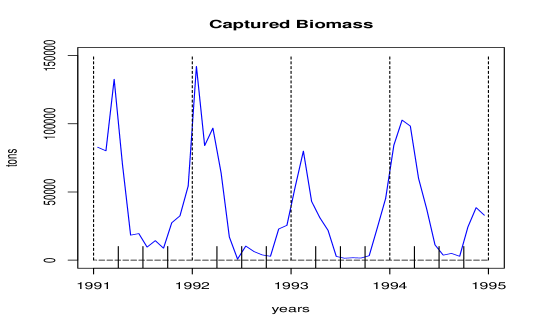
Figure 1. Captures of anchovy and common sardine (1991–1995) in southern Chilean coast [11]. The period with the largest fishing mortality is the summer, while the lowest one corresponds to the closed season.

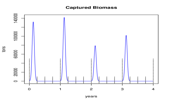
Figure 2. Idealized scheme of the previous figure: intense fishing season alternated by absolute closures of nine months. If the lenght of openings are small compared with closures and the harvested stock is large, it can be considered as a pulse.

The problem of determining the lenght of a closure (in a context of short–term open seasons with intense fishing effort) ensuring the bioeconomical sustantability is a complex issue: indeed, short term closures followed by intense captures could induce an overexploitation of the resource. On the other hand, long–term closures could have some unexpected drawbacks as: i) Bio–sustainable economic rent with negative average [6]. ii) Promotion of negative indirect effects [3], [17] when the resource is a top predator. An example is given by the closure (1989–1992) of the mollusk Concholepas concholepas in the chilean coasts [27]. iii) The phenomenon known as race for fish: fishing units try to outdo one another in fishing power and efficiency during the brief openings [7].

1.2. Mathematical modeling

In this paper, we will assume that the fishery process has two different time–scales. In the first scale (closed seasons), the growth of a single unstructured marine resource is described by using ordinary differential equations. Nevertheless, as the capture has a duration considerably shorter than the closures lenght, every open season will be considered as an instant of capture, i.e., a term of a sequence $\{t_{k}\}_{k}$, this is the second scale (See Figure 2). In consequence, the global process will be described by an impulsive differential equation, IDE (see e.g., [16], [24] for details).

IDE equations have been used in the mathematical modeling of processes involving impulsive harvesting: e.g., [2], [4], [5], [14], [32], [33], [34], [35] (see [22] and [31] for more applications of IDE to bioeconomics and ecological processes respectively). In all these references, the following sequence of harvest instants is employed:

(1.1) $$t_{k}=k\tau\quad\textnormal{with}\quad k=0,1,\ldots,\quad\textnormal{and}\quad\tau>0,$$

which implies that $\tau=t_{k+1}-t_{k}$ is the time between two consecutive captures.

This paper follows a different approach. Indeed, we introduce a new sequence $\{t_{k}\}_{k}$ of harvest instants, where the time for the $(k+1)$–th capture is determined by the amount of the biomass harvested at $k$–th time (which will be denoted by $x(t_{k})$). This leads to a length of closed season determined by

(1.2) $$t_{k+1}-t_{k}=\tau(x(t_{k})),$$

where $\tau(\cdot)$ is some function depending on the amount of the biomass captured at $t=t_{k}$. In consequence, the biomass harvested at time $t=t_{k}$ will determine the instant of the next capture. The idea is to define a length closure such that a bigger capture leads to a longest closure and by assuming broad and realistic properties on per capita growth rate and product function, we will find sufficient conditions ensuring a sustainable production, i.e., the existence of a globally stable periodic trajectory.

This approach has been introduced in [9], where it is pointed out that the resulting model is a new type of IDE equations, namely IDE with impulses dependent of time (IDE–IDT) and an introductory theory is presented.

1.3. Outline

In section 2, we construct a model of fishery with closed seasons and pulse captures, which is described by an IDE–IDT. In section 3, we study some basic properties of the resulting IDE–IDT. The main results concerning the sustainability of the resource are presented in section 4. A numerical example is presented in section 5.

2. The model

A classical mathematical model of a fishery with closed seasons has to describe the following bioeconomic processes: i) The growth of the resource (e.g., a single marine species). ii) The production function. iii) The length of the closures.

2.1. Natural rate of growth

The growth of the biomass in the close season will be described by the ordinary differential equation:

(2.1) $$x^{\prime}(t)=x(t)\,r(x(t)),\quad\textnormal{for any}\quad t\in(t_{k},t_{k+1}),$$

where $\{t_{k}\}$ denotes an increasing sequence of harvest instants.

Growth hypotheses (G)

• Density–dependence. The per capita rate of growth $r\colon[0,K]\to[0,+\infty)$ is a derivable and strictly decreasing function of the biomass. In addition, we assume $r(0)=r_{0}>0$ and $r(K)=0$.

• Bounded variation. The rate $r\colon[0,K]\to[0,+\infty)$ has lowerly bounded derivative, i.e., there exists $\rho>0$, such that $-\rho\leq r^{\prime}(x)<0$.

Remark 1.

The property of derivability stated in (G1) is a technical assumption. Nevertheless, in [28], some statistical results support the negative correlation between per capita rate of growth and biomass. Notice that, $0$ and $K$ are the unique equilibria of (2.1) and $[0,K]$ is a positively invariant set.

Remark 2.

(G2) implies that the function $x\mapsto x\,r(x)$ satisfies the local Lipschitz condition when $x\in[0,K]$. Hence, the solutions of (2.1) are unique to the right and depend continuously on initial condition to the right.

An example of growth rates satisfying (G) are given by the family:

(2.2) $$r(x)=r_{0}\Big{(}1-\Big{[}\frac{x}{K}\Big{]}^{\theta}\Big{)}^{\beta},\quad\textnormal{with}\quad\theta\geq 1\quad\textnormal{and}\quad\beta\geq 1,$$

which generalizes the logistic Verhulst–Pearl per capita rate (see e.g., [29]).

Another example is given by the function [26]:

(2.3) $$r(x)=r_{0}\frac{K-x}{K+cx},\quad\textnormal{with}\quad c>0,$$

which was used, for example, to describe the growth of Daphnia Magna.

2.2. Fishing mortality

The fishing mortality (see [21, p.102]) is the fraction $F\in[0,1]$ of average population taken by fishing. In order to estimate it, we emphasize that there are two possible scenarios: an open season one, where the fishing is allowed all the time, and a restricted process (closed season), where the fishing is forbidden.

The global fishing process is studied with two time scales: the first one describes the close season and only considers the growth of biomass summarized by (2.1) with assumptions (G). The second scale concentrates the fishing mortality by considering the captures as pulses defined in a sequence of harvest instants $\{t_{k}\}$, obtaining:

(2.4) $$F=\frac{x(t_{k})-x(t_{k}^{+})}{x(t_{k})}=\frac{H(x(t_{k}))}{x(t_{k})},$$

where $x(t_{k}^{+})$ is the after $k$–th capture biomass and $H(\cdot)$ describes the capture function in the biomass level at $t_{k}$. From (2.4), we can see that fishing mortality can be seen as a measure of catch per unit of biomass (CPUB).

For convenience, let us define the impulse action $I\colon[0,K]\mapsto[0,K]$, as follows:

(2.5) $$I(x)=x-H(x)=(1-F)x.$$

In order to relate fishing mortality with the input factors (capital and labor) deployed along the fishing process, the continuous modeling literature has introduced the concept of fishing effort, which is a rate describing the number of boats, traps, hooks, technicians, fishermens, etc., per time (see e.g., [1], [6], [21]).

In an impulsive modeling framework, if the punctual fishing effort is denoted by $E>0$, a bounded scalar measure, it is expected to describe (2.4) by a functional relation $F=\phi(E,x(t_{k}))$, which, combined with (2.1) and (2.5), allows to introduce the complementary evolution law:

(2.6) $$x(t^{+})=I(x(t))=\big{(}1-\phi(E,x(t))\big{)}x(t),\quad\textnormal{with}\quad t=t_{k}.$$

We point out that the practical estimation of $E$ and $\phi(\cdot,\cdot)$ are complicated matters in bioeconomic theory and we refer the reader to [1], [6], [30] for details.

Harvest hypotheses (H):

• Impulsive action. $I(\cdot)$ is a derivable and increasing function.

• Elasticity. If $\Delta x\to 0$, then:

  (2.7) $$\frac{\Delta H/H}{\Delta x/x}\to\frac{H^{\prime}(x)\,x}{H(x)}\geq 1,$$

  for any $x\in(0,K]$. This is, a percentage change in the resource biomass determines a percentage change bigger than or equal in the captured amount. Notice that, if the yield elasticity respect to the biomass is bigger or equal than one, then $I(\cdot)$ is inelastic or unitary.

Remark 3.

The property (H1) combined with (2.6) says that:

$$x\frac{\partial\phi}{\partial x}(E,x)\leq 1-\phi(E,x)\quad\textnormal{for any}\quad x\in[0,K].$$

Remark 4.

The property (H2) says that a fixed punctual fishing effort is more productive at higher resource availability. In addition, by using (2.5), we can prove that (H2) is equivalent to

$$\frac{I^{\prime}(x)\,x}{I(x)}\leq 1,\quad\textnormal{and}\quad\frac{\partial\phi}{\partial x}(E,x)\geq 0,\quad\textnormal{for any}\quad x\in(0,K].$$

Remark 5.

Notice that, the called Cobb–Douglas production function can be interpreted by a fishing mortality $\phi(E,x)=qE^{\alpha}x^{\beta-1}$ with $q>0$, $\alpha>0$ and $\beta>0$. It is easy to see that hypotheses (H) are verified when $\beta\geq 1$. An important case is the Schaefer assumption [25], corresponding to $\beta=1$ and $\alpha=1$, i.e., the parametrization is linear with respect to the fishing effort and biomass.

2.3. Length of the closures

There exist a third evolution law governing the dynamics, which determine the sequence $\{t_{k}\}$ of harvest instants. It is the first order recurrence that follows:

(2.8) $$\Delta\,t_{k}=t_{k+1}-t_{k}=\tau(I(x(t_{k}))),$$

where $\tau:[0,K^{*}]\to[0,+\infty)$, with $K^{*}=I(K)$.

As it can be observed in (2.8), the length of the next closure, namely $\Delta t_{k}$, is a function $\tau(\cdot)$ of the stock after the $k$–th harvest and allows to establish an automatic regulation of the dynamics by closed seasons. Here, we only introduce a theoretical proposal and we do not deal with the problems of implementation, for instance, those relating to the estimation of data requirred to define the length of the closed seasons.

2.4. The equation model

The dynamics determined by the combination of equations (2.1), (2.4) and (2.8) is formalized by the impulsive differential equation:

(2.9) $$\left\{\begin{array}[]{llll}x^{\prime}(t)&=&x(t)r(x(t)),&t\neq t_{k},\\ x\,(t^{+})&=&I(x(t)),&t=t_{k},\\ \Delta t_{k}&=&\tau(I(x(t_{k}))),&k\geq 0,\\ \end{array}\right.$$

where $(t,x)\in[0,+\infty)\times[0,+\infty)$.

This type of impulsive differential equation is denoted as Impulsive Differential Equations with Impusive Dependent Times (IDE–IDT), which have been introduced by Córdova–Lepe in [9] and its novelty with respect to classic impulsive differential equations is that the sequence of impulse instants is determined by the process dynamics: the harvested stock $I(x(t_{k}))$ will determine the next harvest time $t_{k+1}$. Indeed, the sequence of harvest times is described by:

(2.10) $$t_{k+1}=t_{k}+\tau(I(x(t_{k}))),\\$$

where the biomass $x(t)$ is abruptly reduced to $x(t^{+})=x(t)-I(x(t))$ at $t=t_{k}$.

There exists several models of pulse harvesting of a renewable resource (not uniquely restricted to fisheries) described by impulsive equations, e.g.,: [2], [4], [5], [8] and [32] consider a resource with logistic growth rate, [35] considers a generalized logistic growth. In addition, Gompertz models (which, not satisfy (G2)) have been studied in [5], [14]. Nevertheless, these works consider a fixed time between two harvest processes, which is equivalent to consider $\tau(\cdot)$ as a constant function.

We point out that impulsive models having sequences similar to (2.10) have also been introduced in [20] by Karafyllis in an hybrid control theory setting and are named hybrid systems with sampling partition generated by the system.

3. The impulsive system (2.9)

Given a first harvest time $t_{0}\in\mathbb{R}$ and a biomass level $x_{0}\in[0,K]$, then the existence, uniqueness and continuability of the solution of (2.9), with initial condition $(t_{0},x_{0})$, can be deduced from [9]. Indeed, we know any solution is a piecewise continuous function having first kind discontinuities at the harvest instants $t=t_{k}$ ($k=0,1,2,\cdots$). In addition, we point out that different initial conditions will determine different sequences of harvest instants.

3.1. Basic properties

In the study of (2.9), it will be necessary to consider the initial value ordinary associated problem:

(3.1) $$\left\{\begin{array}[]{l}z^{\prime}(t)\hskip 3.69899pt=z(t)r(z(t)),\\ z(\sigma_{0})=v,\quad\textnormal{with}\quad(\sigma_{0},v)\in\mathbb{R}\times[0,K].\end{array}\right.$$

Definition 1.

The unique solution of (3.1) will be denoted by $t\mapsto\varphi(t;\sigma_{0},v)$, for any $t\geq\sigma_{0}$, and $\varphi(\sigma_{0};\sigma_{0},v)=v$.

Observe that given $v\in[0,K]$, the function $\varphi(\cdot;\sigma_{0},v)\colon[\sigma_{0},+\infty)\to[0,K]$ satisfies:

(3.2) $$\varphi(t;\sigma_{0},0)=0\quad\textnormal{and}\quad\frac{\partial\varphi}{\partial v}(t;\sigma_{0},v)\geq 0.$$

Let $x(\cdot)$ be the solution of (2.9) with initial condition $(t_{0},x_{0})$, which determines the sequence $\{(t_{k},x(t_{k}))\}_{k}$. Since (2.9) is an ODE on $(t_{k},t_{k+1}]$, we can deduce that $x(\cdot)$ coincides with the unique solution $\varphi(\cdot,t_{k},I(x(t_{k})))$ of (3.1) on $(t_{k},t_{k+1}]$.

By using Definition 1, it follows that

$$\varphi(\sigma+t_{k};t_{k},I(x(t_{k})))=I(x(t_{k}))\exp\Big{(}\int_{t_{k}}^{\sigma+t_{k}}r\big{[}\varphi(s;t_{k},I(x(t_{k})))\big{]}\,ds\Big{)},$$

$$\hskip 103.85237pt=I(x(t_{k}))\exp\Big{(}\int_{0}^{\sigma}r\big{[}\varphi(s+t_{k};t_{k},I(x(t_{k})))\big{]}\,ds\Big{)}.$$

Finally, uniqueness of solutions implies $\varphi(s+t_{k};t_{k},I(x(t_{k})))=\varphi(s;0,I(x(t_{k})))$, which leads to:

(3.3) $$\varphi(\sigma+t_{k};t_{k},I(x(t_{k})))=I(x(t_{k}))\exp\Big{(}\int_{0}^{\sigma}r\big{[}\varphi(s;0,I(x(t_{k})))\big{]}\,ds\Big{)},$$

for any $\sigma\in[0,\tau(I(x(t_{k}))]$.

By using (2.10), it follows that at $\sigma=\tau(I(x(t_{k})))$ (i.e., at $t=t_{k+1}$), the solutions of (2.9) satisfy the one dimensional map:

(3.4) $$x(t_{k+1})=f(x(t_{k})),$$

where the function $f\colon[0,K]\to[0,K]$ is described as follows:

(3.5) $$f(x)=F(I(x)),\quad\textnormal{with}\quad F(y)=y\,\exp\Big{(}\int_{0}^{\tau(y)}r[\varphi(s;0,y)]ds\Big{)}.$$

Notice that Eq.(2.6) implies $f(0)=0$. This fact will have important consequences when studying the asymptotic behavior of (2.9).

3.2. Special solutions of (2.9) and bio-economic interpretation

Let us introduce the straightforward result:

Lemma 1.

Any positive fixed point $u^{*}\in(0,K]$ of the map (3.4) defines a piecewise–continuous $\tau(I(u^{*}))$–periodic solution $t\mapsto u^{*}(t)$ of (2.9), namely, the $u^{*}$–associated solution. In addition, the fixed point $u^{*}=0$ of the map (3.4) defines a constant null solution of (2.9).

The existence of a $\tau(I(u^{*}))$–periodic solution can be interpreted as a fishery strategy with harvest instants uniformly distributed in time. There exists different stability definitions for these solutions (see e.g., [9] and [20]). In this context, we will follow the ideas stated in [10]:

Definition 2.

The $u^{*}$–associated solution of (3.4) is locally asymptotically stable if there exists $\delta>0$ such that for any solution $t\mapsto x(t)$ of (2.9) with initial condition $x(0)$ satisfying $|x(0)-u^{*}|<\delta$, it follows that:

$$\lim\limits_{k\to+\infty}|x(t_{k})-u^{*}|=0,$$

where $\{t_{k}\}$ is the corresponding sequence of harvest instants associated to $x(0)$.

Definition 3.

The $u^{*}$–associated solution of (3.4) is globally asymptotically stable if for any solution $t\mapsto x(t)$ of (2.9) with initial condition $x(0)>0$, it follows that:

$$\lim\limits_{k\to+\infty}|x(t_{k})-u^{*}|=0.$$

Observe that the asymptotic stability of a $\tau(I(u^{*}))$–periodic solution implies the ecological sustainability of the fishery. On the other hand, the asymptotic stability of the null solution implies the future resource extinction.

4. Sustainability conditions

4.1. General result

Theorem 1.

Let us assume that (G),(H) and the closed season hypotheses:

• Growth type. The function $\tau\colon[0,K^{*}]\to[0,+\infty)$ is derivable and decreasing, such that $\tau(K^{*})=0$.

• Initial condition. The initial value $\tau_{0}=\tau(0)$ satisfies

  (4.1) $$\tau_{0}\leq\frac{1}{\rho K+r_{0}}\ln\Big{(}1+\frac{1}{1-\phi(E,0)}\Big{(}1+\frac{r_{0}}{\rho K}\Big{)}\Big{)}.$$

• Main condition. The following inequality:

  (4.2) $$|\tau(z_{2})-\tau(z_{1})|<\frac{1}{r_{0}}\left\{\ln\left(\frac{z_{2}}{z_{1}}\right)-m(z_{2}-z_{1})\right\},$$

  is verified for $0<z_{1}<z_{2}<I(K)=K^{*}$ and $m=\rho[e^{\alpha\tau_{0}}-1]/\alpha$, with $\alpha=\rho K+r_{0}$.

are satisfied.

Then:

• If $e^{\tau_{0}r_{0}}(1-\phi(E,0))<1$, then the resource–free solution of (2.9) is globally asymptotically stable (extinction case).

• If $e^{\tau_{0}r_{0}}(1-\phi(E,0))>1$, then there exists a unique initial condition $x^{*}=f(x^{*})\in(0,K)$ –with $f(\cdot)$ given by (3.4)– defining a $\tau(I(x^{*}))$–periodic globally asymptotically stable trajectory (sustainable case).

Remark 6.

Notice that (C3) gives us a range of graphic possibilities for the choice of function $\tau(\cdot)$. Moreover, (4.1) implies that the right side of (4.2) is non negative for any $z\in[0,K^{*}]$.

Remark 7.

If (C2) is verified, we can see that $e^{\tau_{0}\,r_{0}}(1-\phi(E,0))>1$ implies

$$\frac{1}{r_{0}}|\ln(1-\phi(E,0))|<\tau_{0}\leq\frac{1}{\rho K+r_{0}}\ln\Big{(}1+\frac{1}{1-\phi(E,0)}\Big{(}1+\frac{r_{0}}{\rho K}\Big{)}\Big{)}.$$

In consequence, the left inequality says that there exists a trade–off between the fishing effort $E$ and the maximal lenght of a closure $\tau_{0}$ ensuring the fishery sustaintability. In addition, observe that the inequality stated above has sense only when $\phi(E,0)\in[0,\phi^{*})\subset[0,1]$, which add a complementary constraint for the fishing effort.

Proof.

The asymptotic behavior of (2.9) is determined by the map (3.4).

Now, we will verify that $f\colon[0,K]\to\mathbb{R}$ satisfies the following properties.

• The map $f$ is derivable and $f(0)=0$,

• The map $f$ is increasing and $f(K)<K$,

• For any $x\in(0,K]$ it follows that:

  $$0\leq\frac{xf^{\prime}(x)}{f(x)}<1.$$

Indeed, a) is straightforward consequence from (2.6) combined with $f^{\prime}(x)=F^{\prime}(I(x))\,I^{\prime}(x)$, where $F^{\prime}(y)$ is defined by:

$$\exp\Big{(}\int_{0}^{\tau(y)}r[\varphi(s;0,y)]\,ds\Big{)}\Big{\{}1+y\,\Big{(}r[\varphi(\tau(y);0,y)]\,\tau^{\prime}(y)+\int_{0}^{\tau(y)}\frac{\partial r}{\partial y}[\varphi(s;0,y)]\,ds\Big{)}\Big{\}}.$$

Let us verify that $f^{\prime}(0)=e^{\tau_{0}r_{0}}I^{\prime}(0)$ is consequence from (G1),(H1),(C2) and (3.2). Now, by using (H1), we observe that b) follows if $F^{\prime}(y)>0$ for any $y\in[0,K]$. When dropping the exponential factor of $F^{\prime}(\cdot)$, we only have to prove that

(4.3) $$1+y\,\Big{(}r[\varphi(\tau(y);0,y)]\,\tau^{\prime}(y)+\int_{0}^{\tau(y)}\frac{\partial r}{\partial y}[\varphi(s;0,y)]\,ds\Big{)}>0$$

for any $y\in[0,K]$.

By hypotheses (G) and (C1), combined with $\frac{\partial\varphi}{\partial y}(s;0,y)>0$ for any $s\in[0,\tau(y)]$, we can observe that inequality (4.3) can be deduced from:

(4.4) $$1>y\,\Big{(}r_{0}\,|\tau^{\prime}(y)|+\rho\,\int_{0}^{\tau(y)}\frac{\partial\varphi}{\partial y}(s;0,y)\,ds\Big{)}.$$

By integral representation of $\varphi(s;0,y+h)$ and $\varphi(s;0,y)$, with $s\in[0,\tau(y)]$ and $h>0$ sufficientl small, the Gronwall inequality implies that

$$\left|\varphi(s;0,y+h)-\varphi(s;0,y)\right|\leq|h|\,e^{(\rho\,K+r_{0})s},$$

for any $s\in[0,\tau(y)]$. Indeed, $\frac{\partial\varphi}{\partial y}(s;0,y)\leq e^{(\rho K+r_{0})s}$, with $s\in[0,\tau(y)]$. Therefore, we can reduce our proof to demand the condition that follows:

(4.5) $$y\left(\frac{\rho}{\alpha}\left[e^{\alpha\tau(y)}-1\right]-r_{0}\,\tau^{\prime}(y)\right)<1,\quad\textnormal{where}\quad\alpha=\rho K+r_{0}.$$

We point out that (C3) is equivalent to (4.5). Indeed, when replacing $z_{1}$ and $z_{2}$ by $y$ and $y+h$ ($h>0$) respectively, (4.5) is obtained by letting $h\to 0$. Inversely, since $\tau(y)<\tau_{0}=\tau(0)$, the inequality (4.2) is obtained by integrating (4.5) on $[0,K^{*}]$, with $K^{*}=I(K)$.

To prove that the right side of (4.2) is greater than zero, we observe that

$$\inf\Big{\{}\frac{\ln(K^{*})-\ln(z)}{K^{*}-z}\colon\,\,z\in(0,K^{*}]\Big{\}}=\frac{1}{K^{*}},$$

and $1/K^{*}>m$ is equivalent to (C2). Finally, observe that (H) and (C1) imply $f(K)=I(K)<K$ and property b) follows.

The property c) is equivalent to $x^{2}(f(x)/x)^{\prime}=F^{\prime}(I(x))I^{\prime}(x)x-F(I(x))<0$ for any $x\in(0,K]$. This is verified if and only if for any $x\in(0,K]$, it follows that:

(4.6) $$x\,I^{\prime}(x)\,\left[1+I(x)W^{\prime}(I(x))\right]\exp(W(I(x)))\leq I(x)\,\exp(W(I(x)))$$

where $W(I(x))$ is defined by

$$W(I(x))=\int_{[0,\tau(I(x))]}r[\varphi(s;0,I(x))]\,ds,\quad\textnormal{for}\quad x\in[0,K].$$

Let us recall that

$$W^{\prime}(y)=r[\varphi(\tau(y);0,y)]\,\tau^{\prime}(y)+\int_{0}^{\tau(y)}\frac{\partial r}{\partial y}[\varphi(s;0,y)]\,ds<0,\quad\textnormal{for}\quad y\in(0,K^{*}].$$

By using this inequality, combined with (4.3) and Remark 4, we can deduce that:

(4.7) $$\frac{I^{\prime}(x)\,x}{I(x)}\leq 1<\frac{1}{1-I(x)|W^{\prime}(I(x))|},\quad\textnormal{with}\quad x\in(0,K].$$

By applying Lemma 2 (see Appendix), there are two posibilities for system (3.4) according the sign of

$$1-f^{\prime}(0)=1-e^{\tau_{0}r_{0}}I^{\prime}(0).$$

By Eq.(2.6), we can express the threshold condition for case (a) $f^{\prime}(0)<1$ as $e^{\tau_{0}\,r_{0}}(1-\phi(E,0))<1$ and for case (b) $f^{\prime}(0)>1$ as $e^{\tau_{0}\,r_{0}}(1-\phi(E,0))>1$. So that, the result follows. ∎

4.2. Application to logistic growth

Notice that, in some cases, the one–dimensional map (3.4) associated to the system (2.9) can be defined explicitly and the previous result improved. Indeed, let us consider a marine species with logistic growth, whose exploitation is described by:

(4.8) $$\left\{\begin{array}[]{llll}x^{\prime}(t)&=&rx(t)\Big{(}1-\frac{\displaystyle x(t)}{\displaystyle K}\Big{)},&t\neq t_{k},\\ x\,(t^{+})&=&I(x(t)),&t=t_{k},\\ \Delta t_{k}&=&\tau(I(x(t_{k}))),&k\geq 0.\\ \end{array}\right.$$

Corollary 1.

Let us assume that the impulse action $I(\cdot)$ satisfies (H) and the close season satisfies (C1) and

• Closure condition. The following inequality:

  $$|\tau(z_{2})-\tau(z_{1})|<\frac{1}{r_{0}}\left\{\ln\left(\frac{z_{2}}{z_{1}}\right)+\ln\Big{(}\frac{K-z_{1}}{K-z_{2}}\Big{)}\right\},$$

  is verified for $0<z_{1}<z_{2}<I(K)=K^{*}$.

Then:

• If $e^{r\tau_{0}}(1-\phi(E,0))<1$, then the resource–free solution of (4.8) is globally asymptotically stable (extinction case).

• If $e^{r\tau_{0}}(1-\phi(E,0))>1$, then there exists a unique initial condition $x^{*}=f(x^{*})\in(0,K)$ defining a $\tau(I(x^{*}))$–periodic globally asymptotically stable trajectory (sustainable case).

Proof.

A simple computation shows that (3.4) is equivalent to the one–dimensional map:

(4.9) $$x(t_{k+1})=f(x(t_{k}))=\frac{KI(x(t_{k}))}{I(x(t_{k}))+[K-I(x(t_{k}))]e^{-r\tau(I(x(t_{k})))}}.$$

We will verify that the map (4.9) satisfies the assumptions of Lemma 2 (see Appendix). Firstly, notice that $f(\cdot)$ can be described as follows:

$$f(x)=F(I(x)),\quad\textnormal{with}\quad F(u)=\frac{Ku}{u+[K-u]e^{-r\tau(u)}},$$

and by using (H), it follows that $f(\cdot)$ is derivable and $f(0)=0$.

Secondly, observe that $f^{\prime}(x)=F^{\prime}(I(x))I^{\prime}(x)$. As in the proof of Theorem 1, it follows that $F^{\prime}(u)>0$ (with $0\leq u\leq I(K)=K^{*}$) if and only if (C3’) is verified. By using this fact, combined with (H1), it follows that $f(\cdot)$ is increasing and $f(K)=F(I(K))<K$.

Finally, from (H2) combined with Remark 4, it follows that

$$0\leq\frac{xf^{\prime}(x)}{f(x)}=\frac{xI^{\prime}(x)F^{\prime}(I(x))}{F(I(x))}=\frac{xI^{\prime}(x)}{I(x)}\frac{F^{\prime}(I(x))I(x)}{F(I(x))}\leq\frac{F^{\prime}(I(x))I(x)}{F(I(x))}.$$

By using (C1), it is not difficult to show that $uF^{\prime}(u)<F(u)$ for any $u\in(0,I(K)]$. This fact, combined with the last above inequality implies that $0\leq xf^{\prime}(x)/f(x)<1$ for any $x\in(0,K]$. Now, as $f^{\prime}(0)=e^{r\tau_{0}}(1-\phi(E,0))$, the result is a direct consequence from Lemma 2. ∎

Remark 8.

• The assumption (C3’) is equivalent to the differential inequality $K>-ru(K-u)\tau^{\prime}(u)$ for any $0\leq u\leq I(K)$, which furnishes a way to design admissible functions $\tau(\cdot)$ describing the lengh of open seasons.

• In addition, it is easy to verify that in this case there are no explicit restrictions for $\tau_{0}$ as stated in (C2) (see also Remark 6).

5. Example

Let us consider a fishery with: biomass growth described by the logistic equation, fishing mortality satisfying Schaefer assumption, i.e., $\phi(E,x)=qE$ and closures having lengths determined by the linear function $\tau\colon[0,K^{*}]\to[0,+\infty)$:

(5.1) $$\tau(z)=a(K^{*}-z),\quad\textnormal{with}\quad a>0.$$

By using remarks 1 and 5, it follows that hypotheses (G) and (H) are satisfied. In addition, observe that assumption (C1) is satisfied since $\tau(\cdot)$ is strictly decreasing and $\tau(K^{*})=0$. Moreover, notice that:

$$-ru(K-u)\tau^{\prime}(u)=aru(K-u)\leq arK^{2}/4,$$

and by using statement i) from Remark 8, it follows that (C3’) is satisfied if $a<4/(rK)$.

On the other hand, as $K^{*}=(1-qE)K$ and $\tau_{0}=\tau(0)=a(1-qE)K$, we obtain the threshold:

(5.2) $$\mathcal{E}(qE)=e^{r\tau_{0}}(1-\phi(E,0))=e^{arK(1-qE)}(1-qE),$$

and by Corollary 1, it follows that the resource–free solution of (4.8) is globally asymptotically stable if $\mathcal{E}(qE)<1$. Similarly, there exists a globally asymptotically stable periodic solution if $\mathcal{E}(qE)>1$.

In order to illustrate some properties of the set of punctual fishing efforts $(0,E^{*})$ ($\mathcal{E}(qE^{*})=1$) ensuring sustainability, let us represent the slope of (5.1) as follows:

$$a=\frac{4}{rK}\eta,\quad\textnormal{with}\quad 0<\eta<1.$$

Notice that, to find $E^{*}$ is equivalent to find the unique fixed point $w^{*}=1-qE^{*}$ of the map $w\mapsto e^{-4\eta w}$. In this case, $E^{*}$ is dependent of the parameter $\eta\in(0,1)$, which is positively related to $\tau_{0}$.

It is straightforward to verify that the function $\eta\mapsto E^{*}$ is increasing and concave. This implies that lower values of maximal closure length $\tau_{0}$ leads to narrow ranges of sustainable punctual effort $(0,E^{*})$.

We illustrate this previous results by using the numerical methods developed by Del-Valle [12]. The following parameters are employed:

(5.3) $$r_{0}=0.05\hskip 1.42271pt\textnormal{[time${}^{-1}$]},\quad K=1000\hskip 1.42271pt\textnormal{[tons]},\quad q=1\quad\textnormal{and}\quad\eta=0.25.$$

These values determine $w^{*}\sim 0.567143$ with a respective $E^{*}\sim 0.432857$. The figure shows the biomass curves associated to the following punctual fishing efforts:

(5.4) $$\begin{array}[]{|c|c|c|c|c|}\hline\cr\mbox{Effort}&\mbox{Case 1}&\mbox{Case 2}&\mbox{Case 3}&\mbox{Case 4}\\ \hline\cr\mbox{$E$}&0.1&0.4&0.4329&0.5\\ \hline\cr\end{array}$$

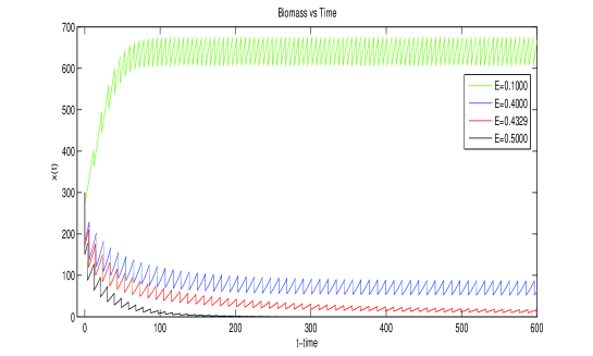
Figure 3. Numerical solution of (4.8) with Schaefer assumption, closure length defined by (5.1) and parameters (5.3). The punctual fishing efforts ensuring sustainability satisfy $E\in(0,0.432857)$.

The Figure 3 shows the evolution of the biomass by considering an initial condition $x(0)=300$ tons and four different punctual fishing efforts. As stated before, we can see an extinction scenario for any punctual effort bigger than $E^{*}$ (this is the case for $E=0.5$). Finally, it can be observed that the lenght of the closure is an increasing function of the punctual effort $E$.

6. Discussion

The mains results (Theorem 1 and Corollary 1) propose sufficient conditions ensuring the ecological sustainability of a simple fishery model with impulsive captures, which can be seen as the trade–off between the fishing effort $E$ and the maximal closure length $\tau_{0}$. The novelty (compared with harvest instants uniformly distributed in time) is to allow a variable length of closures, which has social and economic consequences in a short term.

The proof of Theorem 1 is carried out by constructing a one–dimensional map (3.4), whose asymptotic behavior inherits crucial features of the IDE–IDT equation. In this context, this approach could be extended in several ways. First, notice that assumptions (C2) and (C3) imply that the map (3.4) is strictly increasing. Whe think that it is possible to consider more general maps and obtain less restrictive conditions ensuring convergence towards a fixed point. This remains a future problem and its main difficulty is the hybrid nature of IDE–IDT equations.

Provided that the fishery is sustainable, an important open problem is to find first order conditions on the punctual fishing effort $E$ that maximizes:

$$\frac{\phi(E,x^{*}(E))x^{*}(E)}{\tau([1-\phi(E,x^{*}(E))]x^{*}(E))},$$

the sustainable production per unit time. In other words, the task is the Maximun Sustainable Yield (MSY) problem.

Another extension of this work would be to consider the logistic case (4.8), replacing $r>0$ by a continuous function $r\colon\mathbb{R}\to\mathbb{R}_{+}$. This problem is interesting by a bioeconomic point of view since periodic and Bohr almost periodic functions provide a good tool in order to modeling birth rates with seasonal behavior.

On the other hand, to consider the logistic model (4.8) with almost periodic perturbations has mathematical interest in itself. Indeed, if $r(\cdot)$ is a positive Bohr almost periodic function and $\tau(\cdot)$ is a constant function, it can be proved that there exist a unique almost periodic solution (in the sense of Samolienko and Perestyuk [24]), which is globally asymptotically stable. Nevertheless, there are neither equivalent results nor a study of asymptotic properties when $\tau(\cdot)$ is not constant. A careful development of the qualitative theory for IDE–IDT seems essential to cope with this kind of problems.

Appendix

The following result plays a key role in the proof of Theorem 1:

Lemma 2.

Let us consider the one dimensional map:

(6.1) $$x_{n+1}=f(x_{n}),\quad x_{0}\in[0,K],$$

where the function $f\colon[0,K]\mapsto[0,f(K)]\subset[0,K)$ satisfies the following properties:

• $f$ is derivable and $f(0)=0$,

• $f$ is increasing and $f(K)<K$,

• For any $x\in(0,K]$ it follows that:

  $$0\leq\frac{xf^{\prime}(x)}{f(x)}<1.$$

• If $f^{\prime}(0)<1$ then it follows that $\lim\limits_{n\to+\infty}x_{n}=0$.

• If $f^{\prime}(0)>1$ then there exists a unique fixed point $x^{*}\in(0,K)$ a it follows that $\lim\limits_{n\to+\infty}x_{n}=x^{*}$ for any $x_{0}\in(0,K]$.

Proof.

Case $f^{\prime}(0)<1$: we can verify that there exists $\delta>0$ such that $f(x)<x$ for any $x\in(0,\delta)$. Let us denote by $A$, the set of positive fixed points of $f$. If $A=\emptyset$, by using continuity of $f(\cdot)$ it follows that $f(x)<x$ for any $x\in(0,K]$.

If $A\neq\emptyset$, let us define $\xi=\inf\{A\}$. It is straightforward to verify that:

(6.2) $$\xi>0\quad\textnormal{and}\quad f(x)<x\quad\textnormal{for any}\quad x\in(0,\xi).$$

Now, by using c) we can deduce that $0\leq f^{\prime}(\xi)<1$, which implies the existence of $\delta>0$ such that $f(x)\geq x$ for any $x\in(\xi-\delta,\xi)$, obtaining a contradiction with (6.2).

In consequence $0$ is the unique fixed point in $[0,K]$ and $f(x)<x$ implies that $\{x_{n}\}$ is strictly descreasing and lowerly bounded. Finally, the convergence towards $x=0$ follows from uniqueness of the fixed point.

Case $f^{\prime}(0)>1$: We can verify that there exists $\delta>0$ such that $f(x)>x$ for any $x\in(0,\delta)$. On the other hand, $f(K)<K$ combined with continuity of $f$ imply the existence of a fixed point $x^{*}\in(0,K)$ minimal with this property. Hence, it follows that $f(x)>x$ for any $x\in(0,x^{*})$ and (c) implies that $0\leq f^{\prime}(x^{*})<1$.

In order to prove the uniqueness of $x^{*}$, let us define $g(x)=f(x+x^{*})-x^{*}$ and observe that $g\colon[0,K-x^{*}]\mapsto[0,f(K)-x^{*}]\subset[0,K-x^{*})$ and $g^{\prime}(0)<1$. Hence, the non–existence of fixed points on $(x^{*},K)$ and the property $f(x)<x$ for any $x\in(x^{*},K]$ follows as in the previous case.

If $x_{0}\in(x^{*},K]$ it follows that $\{x_{n}\}$ is strictly descreasing and lowerly bounded by $x^{*}$. On the other hand, if $x_{0}\in(0,x^{*})$ it follows that $\{x_{n}\}$ is strictly increasing and upperly bounded by $x^{*}$. The convergence towards $x^{*}$ follows from the uniqueness of the fixed point in $(0,K)$. ∎

Example: The function $f\colon[0,K]\to\mathbb{R}$ defined by $f(x)=\lambda x/(a+x)$ with $a>1$ and $\lambda<2a$ satisfies straightforwardly the properties a) and b) by choosing $K>a$. Finally, observe that:

$$0\leq\frac{xf^{\prime}(x)}{f(x)}=\frac{1}{a+x}<1,\quad\textnormal{for any}\quad x\geq 0,$$

and c) is verified.

Hence, if $\lambda<a$ (i.e. $f^{\prime}(0)<1$), it follows that the sequence $\{x_{n}\}_{n}$ defined recursively by (6.1) with $x_{0}\in(0,K]$ is convergent to $0$. Otherwise, if $\lambda\in(a,2a)$ (i.e, $f^{\prime}(0)>1$), then the sequence is convergent to $x^{*}=a-\lambda$.

Ackowledgements We would like to express our thanks to professor Luis Cubillos (Universidad de Concepción – Chile) for the data contained in Figure 1. The first author acknowledges the support of Dirección de Investigación UMCE.

References

- [1] L.G. Anderson, The Economics of Fisheries Management. The Blackburn Press, New Jersey, 2004.
- [2] L. Bai, K. Wang, Optimal impulsive harvest policy for time–dependent logistic equation with periodic coefficients. Electronic Journal of Differential Equations 121 (2003).
- [3] E.A. Bender, T.J. Case, M.E. Gilpin, Perturbation experiments in community ecology: theory and tractice. Ecology 65 (1984) 1.
- [4] L. Berezanski, E. Braverman, On impulsive Beverton–Holt difference equations and its applications. J. Diff. Eq. Appl. 10 (2004) 851.
- [5] E. Braverman, R. Mamdani, Continuous versus pulse harvesting for population models in constant and variable environment. J. Math. Biol. 57 (2008) 413.
- [6] C. W. Clark, Mathematical Bioeconomics: The optimal management of renewable resources. John Wiley and Sons, New York, 1990.
- [7] P. Copes, A critical review of the individual quota as a device in fisheries management. Land Economics 62 (1986) 278.
- [8] F. Córdova-Lepe and M. Pinto, Mathematical Bioeconomics. Explotation of resources and preservation. Cubo Mat. Educ., 4 (2002) 49 (Spanish).
- [9] F. Córdova-Lepe, Advances in a Theory of Impulsive Differential Equations at Impulsive-Dependent Times, in: R.P. Mondaini, R. Dilao, (Eds.) Biomat 2006, International Symposium on Mathematical and Computational Biology, World Scientific, 2007, p.p. 343-357.
- [10] F. Córdova–Lepe, R. Del Valle, G. Robledo, A pulse vaccination strategy at variable times depending on incidence. J. Biol. Syst. 19 (2011) 329.
- [11] L. Cubillos, M. Canales, A. Hernández, D. Bucarey, L. Vilugrón, L. Miranda, Fishing power, fishing effort and seasonal and interannual changes in the relative abundance of Strangomera bentincki and Engraulis ringens in the area off Talcahuano, Chile (1990-97). Invest. Mar., 26 (1998) 3 (Spanish).
- [12] R. Del–Valle (2010), Numerical solutions of equations with pulses as models for some biological systems. Presented at poster session of SMB 2010 Annual Meeting and BIOMAT 2010 International Symposium on Mathematical and Computational Biology.
- [13] M.L. Domeier, P.L. Colin, T.J. Donaldson, W.D. Heyman, J.S. Pet, M. Russel, Y. Sadovy, M.A. Samoilys, A. Smith, B.M. Yeeting, S. Smith, Transforming Coral Reef Conservation: Reef Fish Spawning Aggregations Component. Spawning agregation working group report. The Nature Conservancy Hawaii, April 2002. (http://www.scrfa.org/scrfa/doc/fsas.pdf).
- [14] L. Dong, L. Chen, L. Sun, Optimal harvesting policies for periodic Gompertz systems. Nonlinear Analysis Real World Applications 8 (2007) 572.
- [15] H.S. Gordon, Economic theory of a common–property resource: the fishery. Bull.Math.Biol. 53 (1992) 231.
- [16] W.M. Haddad, V. Chellaboina, S.G. Nersesov, Impulsive and Hybrid Dynamical Systems: Stability, Dissipativity, and Control. Princeton University Press, 2006.
- [17] M. Higashi and H. Nakajima, Indirect effects in ecological interaction networks I. The chain rule approach. Math. Biosci. 130 (1995) 99.
- [18] R.E. Johannes, The case for data–less marine resource management: examples from tropical nearshore finfisheries. Trends in Ecology and Evolution. 13 (1998) 243.
- [19] R.E. Johannes and F.R. Hickey, Evolution of village–based marine resources management in Vanuatu between 1993 and 2001. Coastal region and small islands papers 15, UNESCO, Paris, 2004.
- [20] I. Karafyllis, A system–theoretic framework for a wide class of systems I: application to numerical analysis. J. Math. Anal. Appl. 328 (2007) 876.
- [21] J. Kolding, W.U. Giordano, Lecture notes. AdriaMed Training Course on Fish Population Dynamics and Stock Assessment. FAO-MiPAF Scientific Cooperation to Support Responsible Fisheries in the Adriatic Sea. GCP/RER/010/ITA/TD-08. AdriaMed Technical Documents 8. FAO, 2002.
- [22] L. Mailleret, V. Lemesle, A note on semi–discrete modelling in the life sciences. Phil. Trans. R. Soc. A 367 (2009) 4779.
- [23] T.J. Pitcher, E.A. Buchary, U.R. Sumaila, A synopsis of Canadian fisheries. Fisheries Centre, University of British Columbia (http://www2.fisheries.com/archive/publications/reports/canada-syn.pdf).
- [24] A.M. Samoilenko, N.A. Perestyuk, Impulsive differential equations. World Scientific Series on Nonlinear Science, Series A, 14, 1995.
- [25] M.B. Schaefer, Some aspects of the dynamics of population important to the management of commercial marine fisheries. Bull.Math.Biol. 53 (1991) 253.
- [26] F.E. Smith, Population dynamics in Daphnia Magna and a new model for population growth. Ecology 44 (1963) 651.
- [27] W. Stoltz, The management areas in the fishery law: first experiences and evaluation of utility as a management tool for concholepas concholepas, Estud. Oceanol. 16 (1997) 67 (Spanish).
- [28] J. T. Tanner, Effects of population density on growth rates of animal populations, Ecology 47 (1966) 733.
- [29] A. Tsoularis, J. Wallace, Analysis of logistic growth models. Math. Biosci. 179 (2002) 21.
- [30] C.J. Walters, S.J.D. Martell, Fisheries Ecology and Management. Princeton University Press, 2004.
- [31] L. Yang, J.L. Bastow, K.O. Spence, A.N. Wright, What can we learn from resource pulses?. Ecology 89 (2008) 621.
- [32] X. Zhang, Z. Shuai, K. Wang, Optimal impulsive harvesting policy for single population. Nonlinear Analysis Real World Applications 4 (2003) 639.
- [33] Y. Zhang, Z. Xiu, L. Chen, Optimal impulsive harvesting of a single species with Gompertz law of growth, J. Biol. Syst. 14 (2006) 303.
- [34] L. Zhao, Q. Zhang, Q. Yang, Optimal impulsive harvesting for fish populations. J. Syst. Sci. Complex. 16 (2003) 466.
- [35] T. Zhao, S. Tang, Impulsive harvesting and by–catch mortality for the Theta logistic model. App. Math. Comp. 217 (2011) 9412.